Validation of Fiber Breakage in Simple Shear Flow with Direct Fiber Simulation

Abstract

This study aims to use particle level simulation to simulate the breakage behavior of glass fibers subjected to simple shear flow. Each fiber is represented as a chain of rods that experience hydrodynamic, interaction, and elastic effects. In order to validate the approach of the model, the simulation results were compared to simple shear flow experiments conducted in a Couette Rheometer. The excluded volume force constants and critical fiber breakage curvature were tuned in the simulation to gain a better understanding of the system. Relaxation of the fiber clusters and a failure probability theory were introduced into the model to solve the fiber entanglement and thus, better fit the experimental behavior. The model showed agreement with the prediction on fiber length reduction in both number average length and weight average length. In addition, the simulation had a similar trend of breakage distribution compared to a loop test using glass fibers.

1. Introduction

Discontinuous fiber-reinforced polymers play a significant role in industrial applications due to their lightweight performance and lower manufacturing costs [1,2,3]. Currently in the industry, injection molding and compression molding of long fiber-reinforced thermoplastics are widely used to produce parts with outstanding mechanical properties [4]. For example, during injection molding, fiber breakage already starts in the plasticizing section of the machine and continues as the material is forced through the gate and mold filling. There are various modes of fiber breakage—from the melting process to the high shear during mold filling. It has been shown that a big contributor to fiber attrition is the melting zone of the plasticating unit, leading to a significantly shorter fiber length when polymer enters the metering zone from the compression zone [5]. As fiber length is crucial in improving the mechanical performance of a molded product, an increase in fiber length correlates in the increased strength of the product. Researchers have also found that parts are stronger in the direction of fiber alignment if fiber length and volume fraction are increased [6]. During polymer processing, however, fibers in the polymer melt often break because they are subjected to intense viscous forces during flow and deformation. Therefore, it is beneficial to understand the mechanism of fiber breakage during flow, in particular shear flow, which is dominant. This will allow the engineer to optimize the process to reduce the length degradation and, thus, gain better mechanical properties. However, there are still some aspects of processing that are not well understood, which will be addressed further in the paper.

To estimate the mechanical behavior of a product, it is necessary to predict the process-induced fiber breakage. Forgacs et al. [7] proposed in 1959 that the critical shear stress that provokes fiber buckling is described by the fibers’ Young modulus and their geometrical properties. From this, it becomes clear that with high aspect ratios, the fibers tend to break under low loadings. Later, Hinch [8] used the Slender Body theory to obtain the deformation of an ideally elastic particle in shear flow. Using the Couette rheometer, Goris et al. [9] developed an experimental setup in combination with fiber length measurement to obtain repeatable length degradation of glass fibers at different fiber concentration, initial fiber length, residence time, melt temperature, and processing speed. This setup provides good insight into measuring fiber length. However, there is no simulation tool that can accurately predict final fiber length in a molded part and the phenomena of fiber breakage is not fully understood. Therefore, numerical simulation is applied to investigate the phenomena of fiber breakage. Some continuum models which are very different from particle level simulations have been developed to obtain the macroscopic picture of breakage by solving the balance equation of fiber length distribution [2,5]. Phelps et al. [2] presented a quantitative model to describe fiber attrition, which is based on buckling as the driving mechanism for fiber breakage during processing. However, Phelps did not explicitly state that the drag coefficient is independent on fiber concentration, which was shown from the Couette rheometer experiments [5]. To fully understand the micromechanical picture of fiber breakage, particle simulation is necessary to develop to understand the details of concentrated fiber suspension dynamics [10,11,12,13,14]. Single particle models are not accurate enough and well developed to investigate the degradation mechanisms at the fiber level due to expensive computation. Therefore, a particle level model developed at the Polymer Engineering Center (PEC) at the University of Wisconsin-Madison will be extended to gain a better understanding of fiber damage.

In this work, a simulation is conducted via a mechanistic model, to understand the effect of fiber breaking curvature and the magnitude of penalty forces that prevent fiber from overlapping during simulation to the fiber damage under shear flow condition, neglecting the effect of melting. In addition, probability breakage is introduced to the system to increase the reliability of the model and better describe the uncertainty of breakage in numerical terms. Moreover, to relieve the entanglement between fibers when generating an initial fiber cluster used for the simulation, a relaxation step is applied to reduce the initial breakage caused by an unsteady system. Then, the mechanistic model is used to predict fiber breakage in a Couette flow rheometer. By comparing the model’s predictions to the experimental curve, the influence of adjusting parameters in the model to different conditions is assessed.

2. Direct Fiber Model

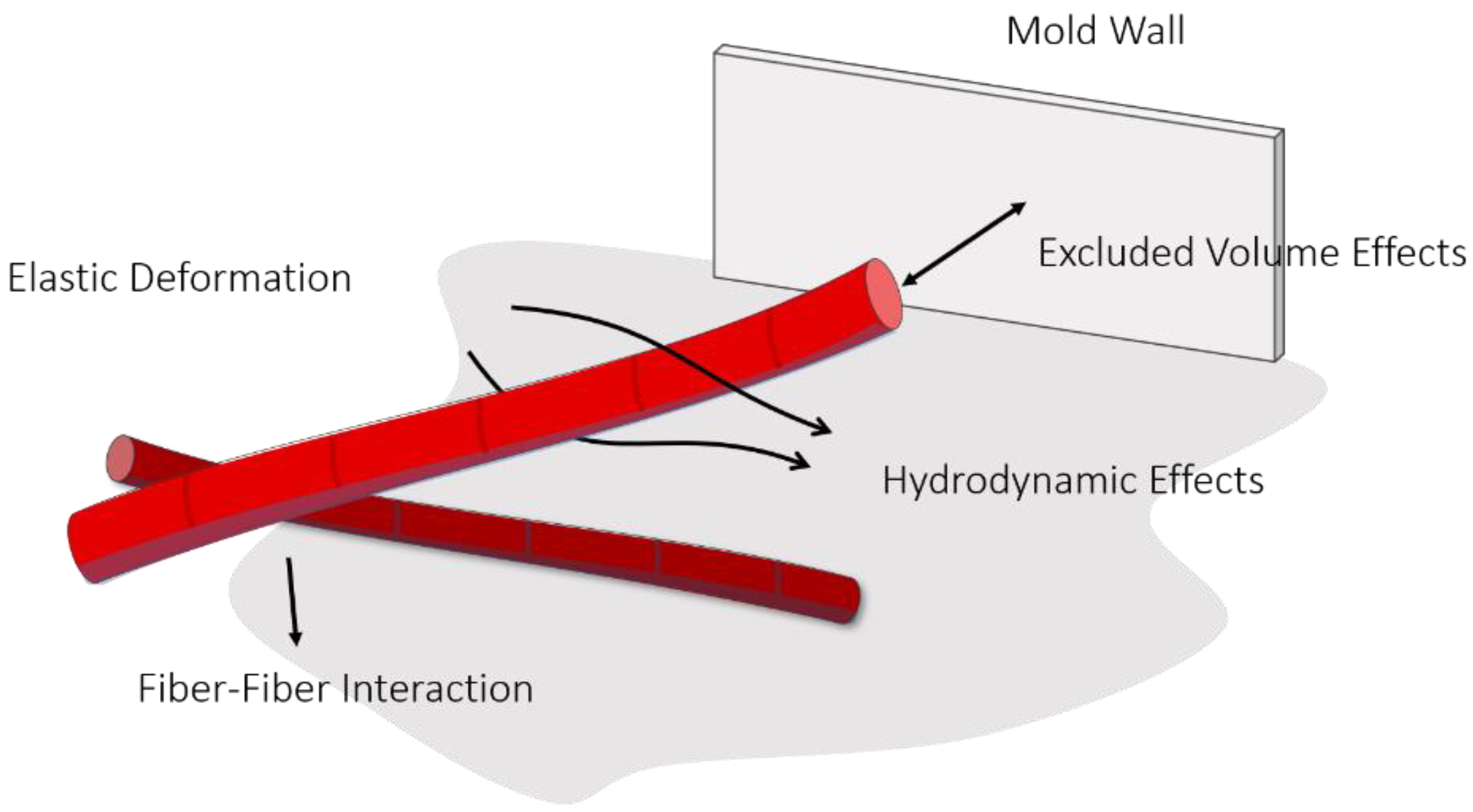
In the mechanistic model, which is based on a work done by Schmid et al. [11], models fibers are chains of rigid cylindrical rods, as shown Figure 1. At each segment node in a fiber, the position $x_i$, the velocity $u_i$ and the angular velocity ${\omega }_i$ are calculated. Additionally, the segments experience hydrodynamic effects, fiber-fiber interaction, excluded volume effects, and elastic deformation within the flow field.

The fibers are immersed in a homogeneous shear flow, which is at a low Reynolds number; therefore, inertial effects can be neglected based on the experiments by Hoffman [15] and Barnes [16]. In addition, long-range hydrodynamic interactions are neglected due to high viscosity for polymers [17]. Furthermore, as fluid forces are not high enough to cause fibers to stretch or have torsional deformation, only bending deformation is included in the model. Buoyant effects are neglected as well [18,19].

The excluded volume force stops fibers from overlapping and is used to model inter-fiber interaction; it is implemented as a discrete penalty method. Discretizing the fibers into more than two nodes or one beam allows fiber bending to occur, where the back coupling from fiber motion to fluid is not considered due to expensive computational cost [18]; the force equilibrium are written as:

$$\underset{\_}{0}={\underset{\_}{F}}_i^H+{\displaystyle \sum }_j{\underset{\_}{F}}_{ij}^C+{\underset{\_}{X}}_i-{\underset{\_}{X}}_{i+1}$$

(1)

where ${\underset{\_}{F}}_i^H$ is the drag forces from the surrounding fluid, ${\underset{\_}{F}}_{ij}^C$ the inter-fiber interaction force with rod $j$, and ${\underset{\_}{X}}_i, {\underset{\_}{X}}_{i+1}$ the intra-fiber forces exerted by adjacent rods.

Likewise, the moment equilibrium is analogous but includes an elastic recovery term ${\underset{\_}{M}}^b$ and a hydrodynamic torque ${\underset{\_}{T}}^H$, where ${\underset{\_}{r}}_{ij}$ describes the shortest distance vector between two segments:

$$\underset{\_}{0}={\underset{\_}{T}}_i^H-{\underset{\_}{r}}_i\times {\underset{\_}{X}}_{i+1}+{\displaystyle \sum }_j{\underset{\_}{r}}_{ij}\times {\underset{\_}{F}}_{ij}^C+{\underset{\_}{M}}_i^b-{\underset{\_}{M}}_{i+1}^b$$

(2)

Additionally, if a fiber has more than one segment, an extra constraint that enforces connectivity between the different segments is used with ${\underset{\_}{u}}_i$, the speed of rod $i$, and angular speed ${\underset{\_}{\omega }}_i$:

$$0={\underset{\_}{u}}_i+{\underset{\_}{\omega }}_i\times {\underset{\_}{r}}_i-{\underset{\_}{u}}_{i+1}$$

(3)

Using a chain of beads to represent the rod-like geometry of a fiber for hydrodynamic effects reduces the complex solution as compared with an ellipsoid geometry [20]. The hydrodynamic force ${\underset{\_}{F}}_i^H$ is calculated as the summation of forces experienced by the beads ${\underset{\_}{F}}_k^H$ and is given as:

$${\underset{\_}{F}}_i^H={\displaystyle \sum }_{k=1}^m{\underset{\_}{F}}_k^H$$

(4)

where ${\underset{\_}{F}}_k^H$ is the hydrodynamic force and $k$ describes the number of beads given by Stokes law:

$${\underset{\_}{F}}_k^H=6\pi \mu a\left({\underset{\_}{u}}_k^{\infty }-{\underset{\_}{u}}_k\right)$$

(5)

where ${\underset{\_}{u}}_k^{\infty }$ is the surrounding fluid velocity, $a$ is the radius of the bead, and ${\underset{\_}{u}}_k$ is the velocity bead $k$, which can also be represented as (${\underset{\_}{u}}_k={\underset{\_}{u}}_i+{\underset{\_}{\omega }}_i\times {\underset{\_}{r}}_k$). This allows the final ${\underset{\_}{F}}_i^H$ equation to be written as shown below:

$${\underset{\_}{F}}_i^H=6\pi \mu a\left({\displaystyle \sum }_{k=1}^m{\underset{\_}{u}}_k^{\infty }-m{\underset{\_}{u}}_i-{\underset{\_}{w}}_i\times {\displaystyle \sum }_{k=1}^m{\underset{\_}{r}}_k\right)$$

(6)

Similarly, the torque exerted on a rod is:

$${\underset{\_}{T}}^H={\displaystyle \sum }_{k=1}^m{\underset{\_}{T}}_k^H$$

(7)

where the hydrodynamic contribution ${\underset{\_}{F}}_k^H$ of bead $k$, where ${\underset{\_}{\mathsf{\Omega }}}_k^{\infty }$ is the vorticity of the surrounding fluid and ${\underset{\_}{\omega }}_k$ is the angular velocity of the bead k.

$${\underset{\_}{T}}_k^H=8\pi \mu a^3\left({\underset{\_}{\mathsf{\Omega }}}_k^{\infty }-{\underset{\_}{w}}_k\right)+6\pi \mu a{\underset{\_}{r}}_k\times \left({\underset{\_}{u}}_k^{\infty }-{\underset{\_}{u}}_i-{\underset{\_}{w}}_i\times {\underset{\_}{r}}_k\right)$$

(8)

By substituting the expression of ${\underset{\_}{T}}_k^H$, the expression of ${\underset{\_}{u}}_k$ into the fluid’s vorticity can be written as:

$${\underset{\_}{T}}^H=8\pi \mu a^3\left({\displaystyle \sum }_{k=1}^m{\underset{\_}{\mathsf{\Omega }}}_k^{\infty }-m{\underset{\_}{w}}_i\right)+6\pi \mu a{\underset{\_}{r}}_k\times \left({\displaystyle \sum }_{k=1}^m\left({\underset{\_}{r}}_k\times {\underset{\_}{u}}_k^{\infty }\right)+{\underset{\_}{u}}_i\times {\displaystyle \sum }_{k=1}^m{\underset{\_}{r}}_k-{\displaystyle \sum }_{k=1}^m{\underset{\_}{r}}_k\times \left({\underset{\_}{w}}_i\times {\underset{\_}{r}}_k\right)\right)$$

(9)

Using the elastic beam theory, the approach below is similar to Schmid [11]. The bending moment of a fiber where the radius of curvature of a beam subjected to pure bending is given by:

$$\frac{1}{\rho }=\frac{M}{EI}$$

(10)

where $M$ is the bending moment, $E$ the Young’s modulus, $\rho$ the radius of curvature of the beam, and $I$ is the inertial moment of the beam’s cross section.

On approximation by linear segments, which is connected with elastic joints, the bending moment will be related to the length of the segment $\ell$ and angle $\alpha$; then:

$${\underset{\_}{M}}_i^b=\frac{\alpha IE}{\ell }\underset{\_}{e}$$

(11)

$$\underset{\_}{e}=\frac{{\underset{\_}{r}}_i\times {\underset{\_}{r}}_{i-1}}{\left|{\underset{\_}{r}}_i\times {\underset{\_}{r}}_{i-1}\right|}$$

(12)

The model also includes mechanical interaction between fibers. The fiber-fiber interaction force is the sum of a normal force and a tangential force, as seen below, where ${\underset{\_}{F}}^N$ is the normal force, and ${\underset{\_}{F}}^T$ is the tangential force representing the friction between rods.

$${\underset{\_}{F}}_{ij}^C={\underset{\_}{F}}_{ij}^N+{\underset{\_}{F}}_{ij}^T$$

(13)

The collision response between fibers is represented as a discrete penalty method [21,22]. The penalty method implemented in the model starts with selecting a force dependent on the penetration distance. The equation below of the excluded volume force is often used in a particle level simulation for fiber suspension [11,23,24], where A and B are parameters [25,26], $d_{ij}$ is the shortest distance between rod $i$ and rod $j$, b is the fiber radius, and ${\underset{\_}{n}}_{ij}$ is the vector along the closest distance between the rods.

$${\underset{\_}{F}}_{ij}^N=A \exp \left[-B\left(\frac{2d_{ij}}{D}-2\right)\right]{\underset{\_}{n}}_{ij}$$

(14)

The force increases exponentially as fibers get closer. In this research, B is chosen as 2 [18], and A is tuned for each system which represent as excluded volume force constant later.

The friction force between segment $i$ and $j$ is calculated as a force in the direction of the relative velocity of the rods and is computed using the equation below, where ${\mu }_f$ is the coulomb coefficient between fibers and $∆u_{ij}$ is the relative velocity between segments $i$ and $j$.

$${\underset{\_}{F}}_{ij}^T={\mu }_f\left|{\underset{\_}{F}}_{ij}^N\right|\frac{∆u_{ij}}{\left|∆u_{ij}\right|}$$

(15)

Due to the non-linear behavior, the model uses the previous time step to calculate future steps. For this reason, the initial time step is zero to avoid the absence of data points.

3. Fiber Deformation and Breakage

In the mechanistic model, bending of a fiber is the only mechanism attributed to fiber deformation. Elongation and shear-deformation due to tensile, compression, and shear loads are neglected. Thus, the bending behavior is implemented with the elastic beam theory. In the model, the forces experienced by the fibers within the polymer matrix, which lead to bending and breaking, are approximated within the linear segments interconnected with flexible joints. To determine the breaking point, the local degree of bending is characterized by the radius of curvature at the connection points of two rods, as shown in Figure 2. Furthermore, the critical curvature is used as an input parameter for the model to initiate fiber breakage. Once a fiber’s segment curvature is below the assigned input parameter, the fiber will break at the joint of two connecting rods.

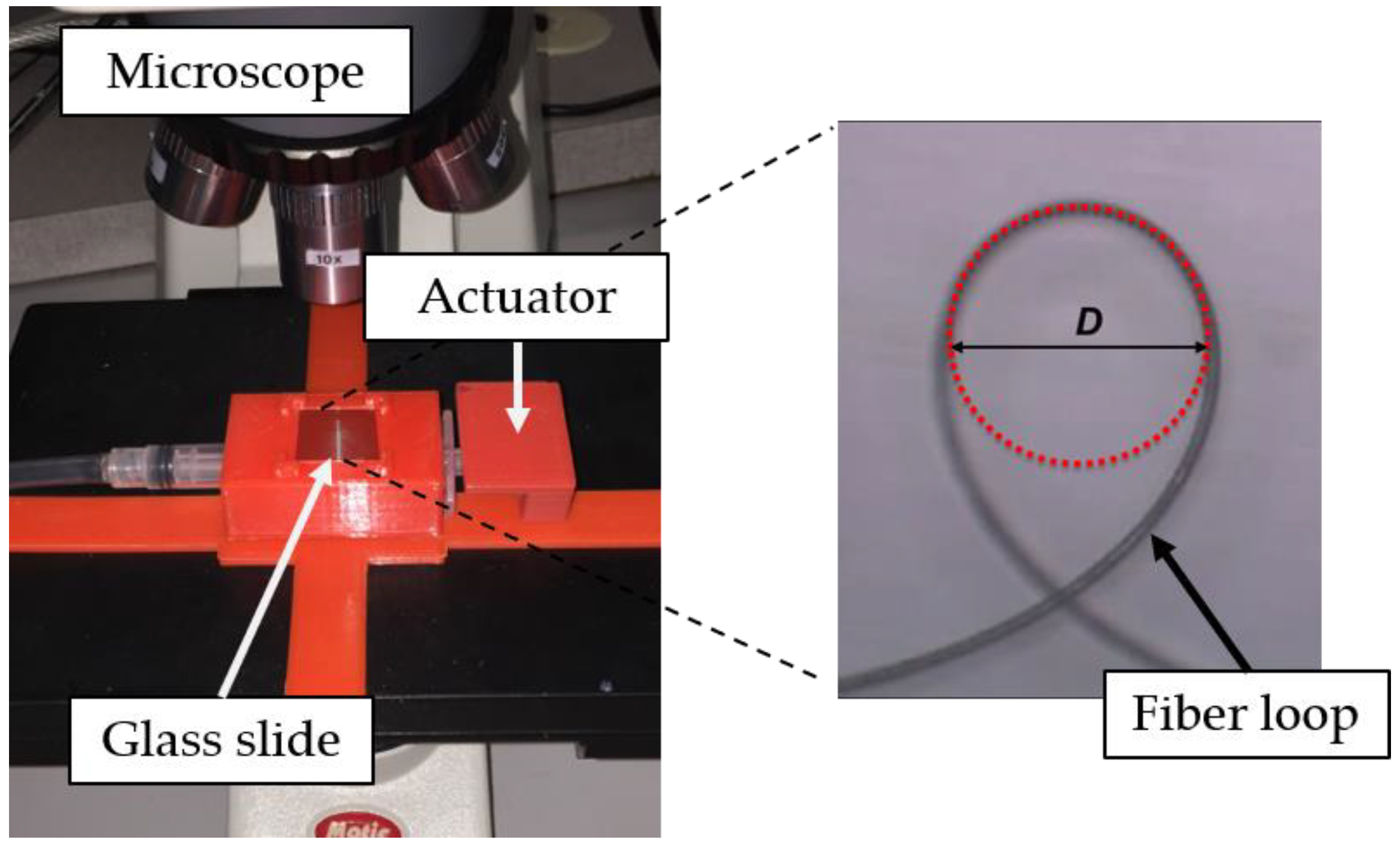
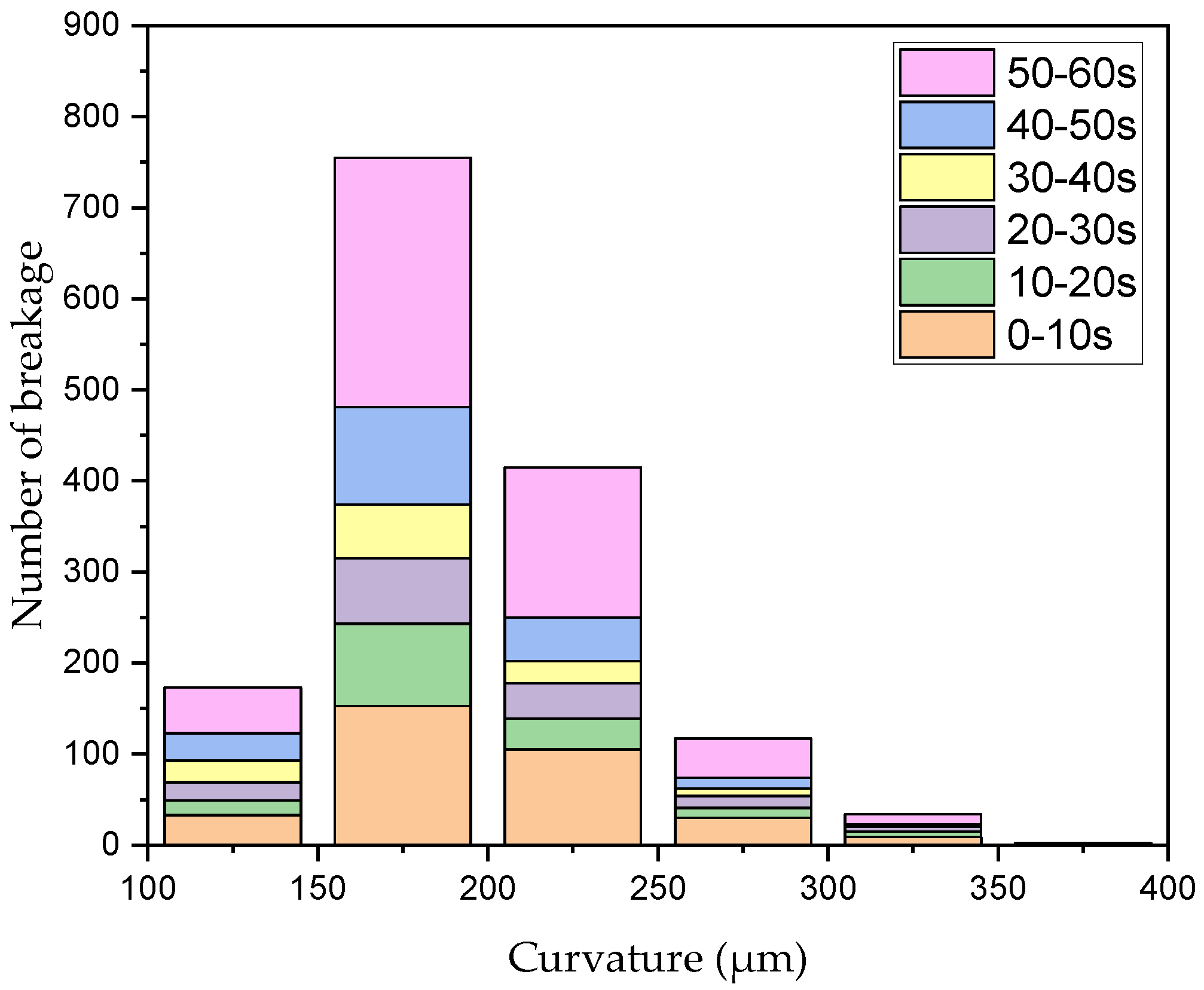
To describe the fiber behavior during breakage under realistic conditions, a bending method was presented by Sinclair [27] using glass fibers. The tensile strength and Young’s modulus were measured by twisting a loop in a fiber and pulling the ends until the loop breaks. To understand the phenomena in a microscopic level of fiber breakage, a test was further developed and improved to obtain the critical radius of curvature for individual fibers [28]. The tested fibers exhibit an elastic modulus of 73,000 N/mm² and a tensile strength of 2600 N/mm². To measure the critical radius of curvature at the break point, the glass fiber was bent into a loop and placed between two glass slides; a drop of glycerin was added to prevent the loop from unfolding and to create a film between the slides. This ensured the fiber would not break due to friction. One end of the loop was fixed to the bottom slide and the other was attached to an actuator. 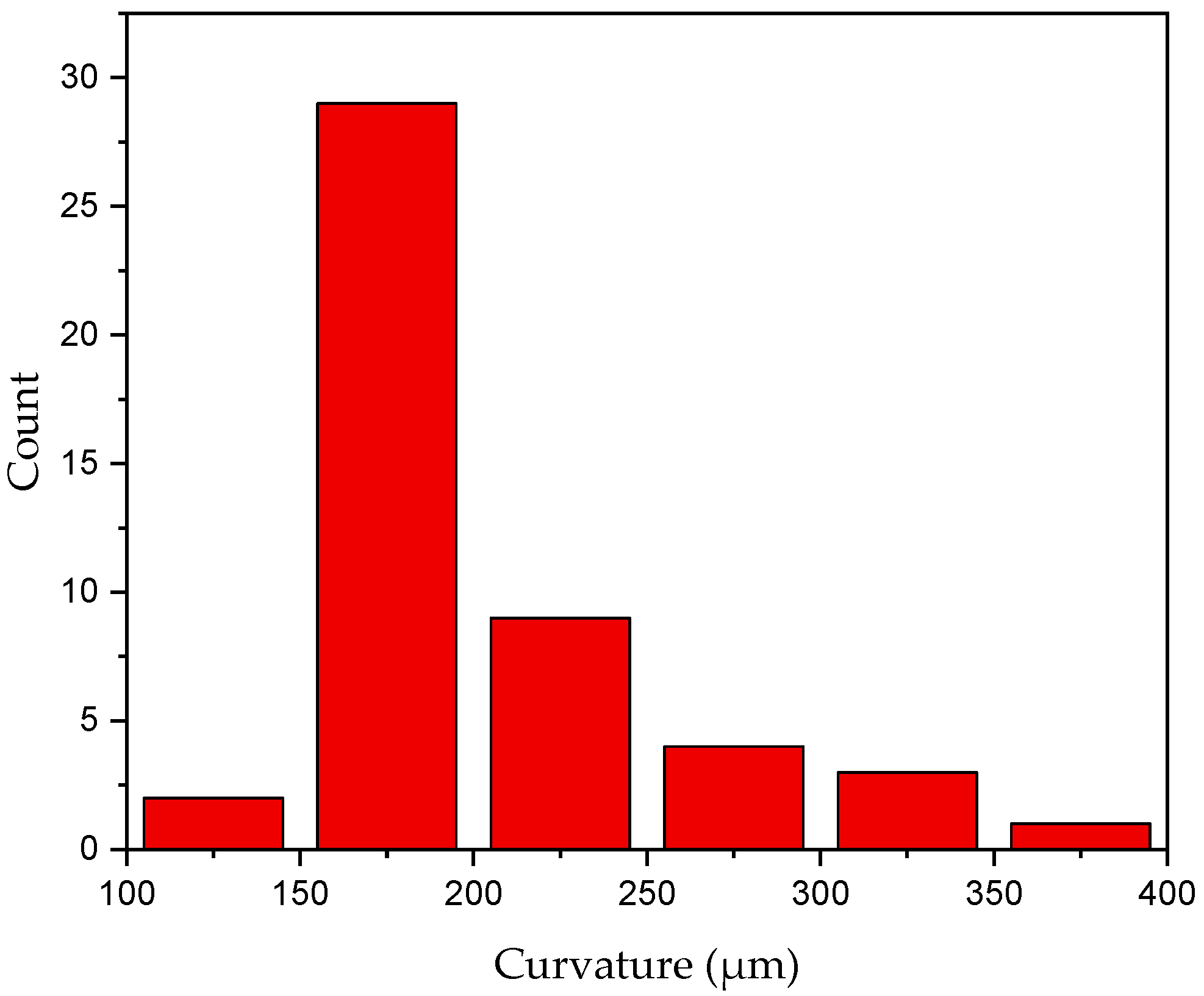The setup was placed under a microscope and a video was recorded while the actuator pulled the end of the fiber until breakage occurred, as seen in Figure 3. The last frame when the loop was still intact was captured and the radius of curvature was measured. A total of 48 experiments were performed and the non-Gaussian distribution resulted in an average value of 204.6 $\mathsf{\mu }\mathrm{m}$ for the critical radius of curvature. The values varied from 119 to 371 $\mathsf{\mu }\mathrm{m}$, as seen in Figure 4.

4. Direct Fiber Simulation

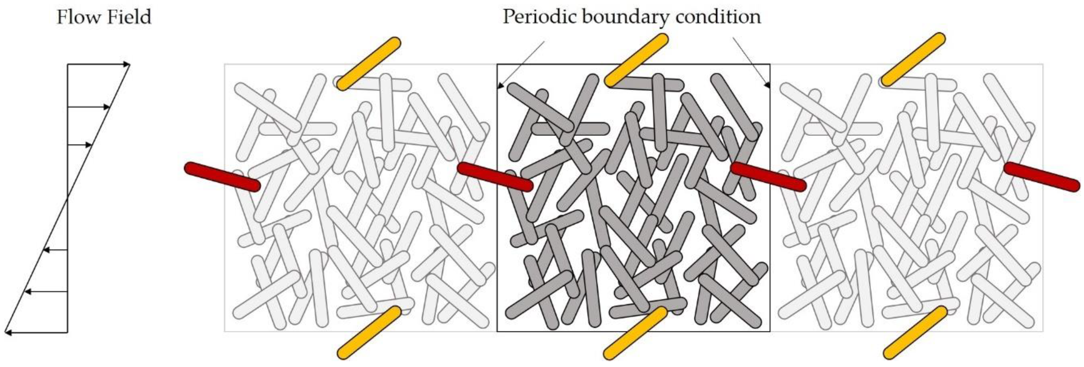
The mechanistic model was first implemented to examine the effect of the excluded volume force constant. To validate the model, the result was compared with the Couette flow experiments using glass fiber-reinforced polypropylene (PP). To set up a simulation, 1000 fibers with equal length of 2.5 mm were placed in a shear cell (Figure 5). The segment length in each fiber is a fixed value of 0.1 mm with aspect ratio of 5.26 to ensure flexible rotation in the flow field [18]. In addition, Lee-Edwards periodic boundaries [29] were applied to all the cell walls to represent periodic conditions during the simulation. A simple shear field with a shear rate of 16.65 s⁻¹ in x–y plane was applied to the polymer matrix, which corresponds to the hydrodynamic forces discussed previously. The material used in this work was SABIC^® STAMAX (Saudi Basic Industries Corporation (SABIC), Riyadh, Saudi Arabia), a reinforced polypropylene material.

Table 1. Constant values of shear cell properties in simulation.

Parameter	Value
Viscosity (Matrix) [Pa s]	200
Shear Rate [s−1]	16.65
Fiber Young’s Modulus [GPa]	73
Fiber diameter [µm]	19
Fiber Weight Fraction [%]	30
Time step [s]	10−6–10−8

shows the physical properties of fibers and the matrix.

Stated in ref. [18], the values of $A$ and $B$ in Equation (14) for a hydrodynamic effect still remain unknown and need to be adjusted for different processing conditions. Values $A$ and $B$ have been chosen empirically, which are usually set in such a way that no fiber intersections are perceived, nor high repulsive forces are created. As suggested by [18], B was chosen to be 2 and $A$ was tuned for each system with the relationship of $shear rate\times viscosity/2$ for the mechanistic model simulation, which is 1665 in this case. 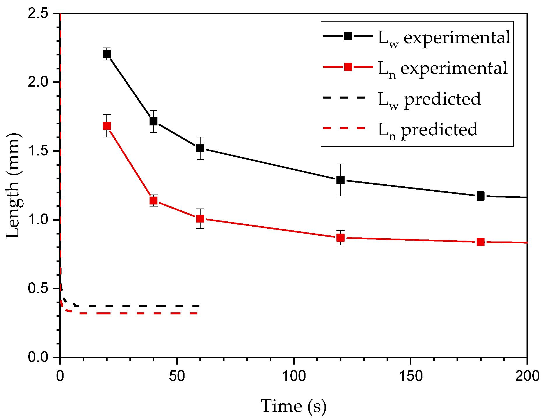Figure 6 shows the number average length ($L_n$) and the weight average length ($L_w$) for the simulation. It is clear that when using the empirical method, breakage occurs too fast, when compared to experimental data. This shows that the traditional algorithm used for the simulation, where $A=1665,$ results in much higher excluded forces than the actual values. This causes fibers to break as they move closer to each other within the cluster. Thus, it is necessary and critical to find a proper repeatable method to determine the value for simulating fiber breakage.

To further validate the model, the critical fiber breaking curvature and excluded volume force constant $A$ were tuned to examine the variation of fiber length reduction.

Table 2. Values varied in simulation.

Parameter	Value
Fiber Critical Curvature [μm]	200, 250, and 300
Excluded Volume Force Constant [-]	250, 500, and 750

shows variables used in the simulation.

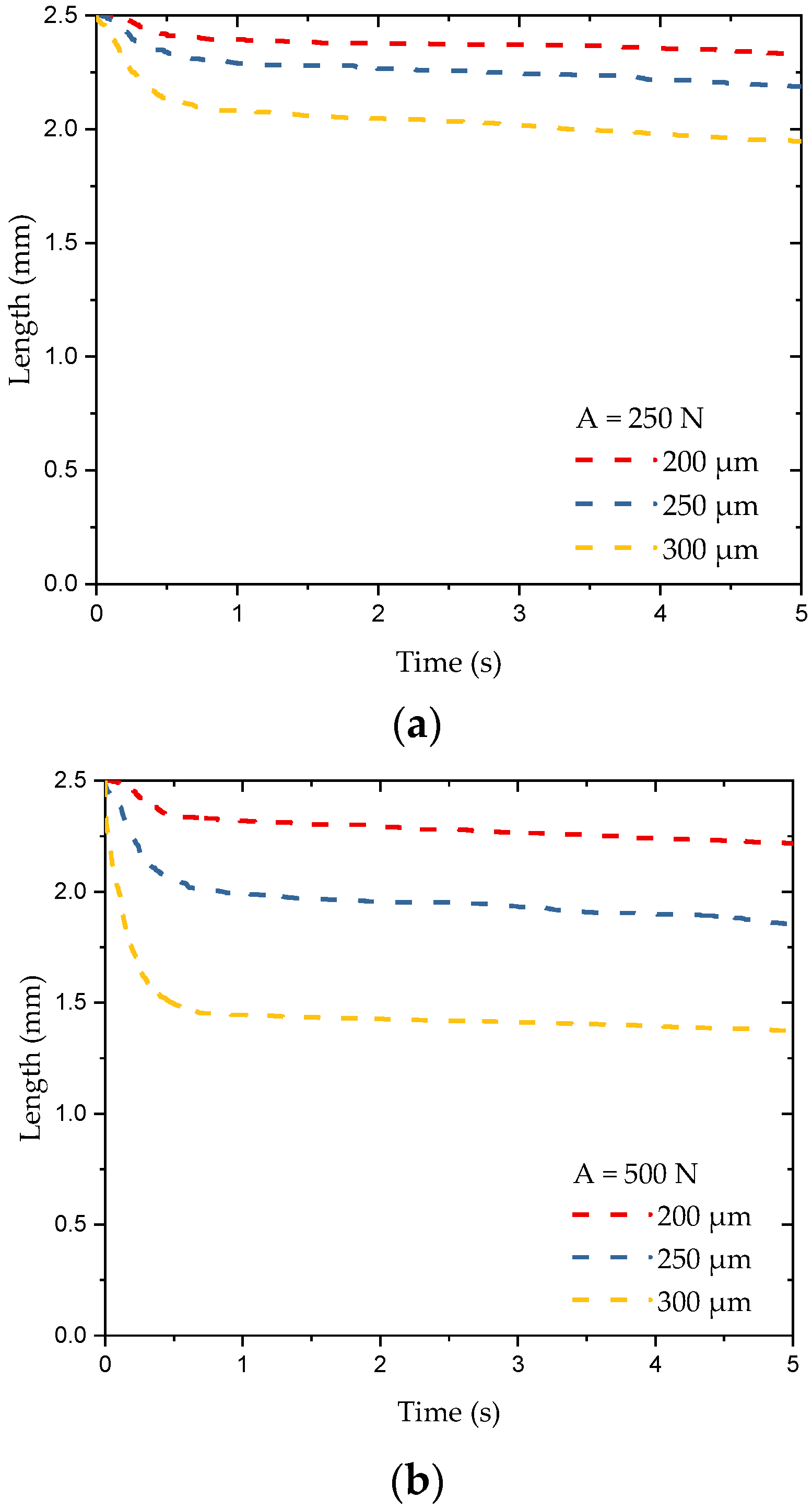
Figure 7 shows the 5 s time evolution of $L_n$ at varying pre-demand breaking curvature from 200$\mathsf{\mu }\mathrm{m}$, 250$\mathsf{\mu }\mathrm{m}$, and 300 $\mathsf{\mu }\mathrm{m}$ while keeping the same excluded volume force constant. As fibers start to bend, they first reach a larger critical curvature and result in a faster rate of breakage. On increasing the force constant, the fiber experiences higher repulsive force as they approach surrounding fibers. 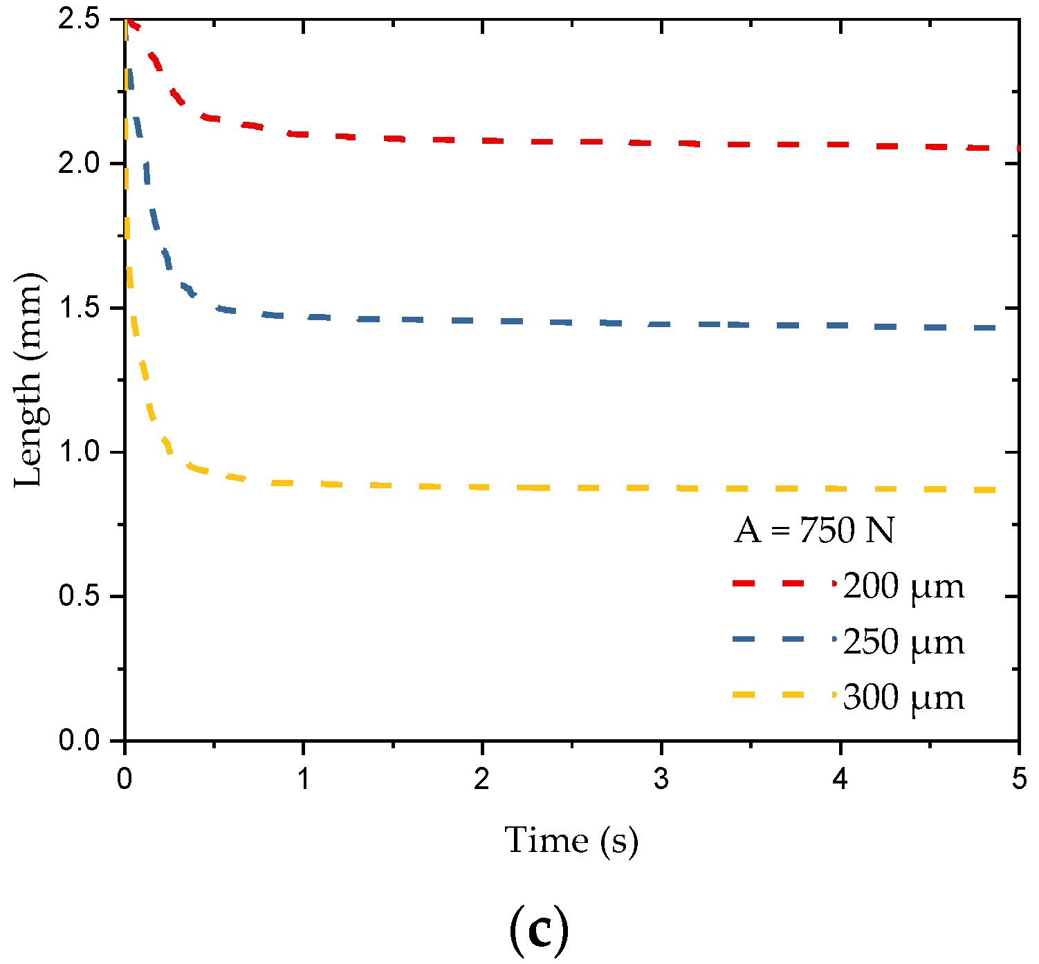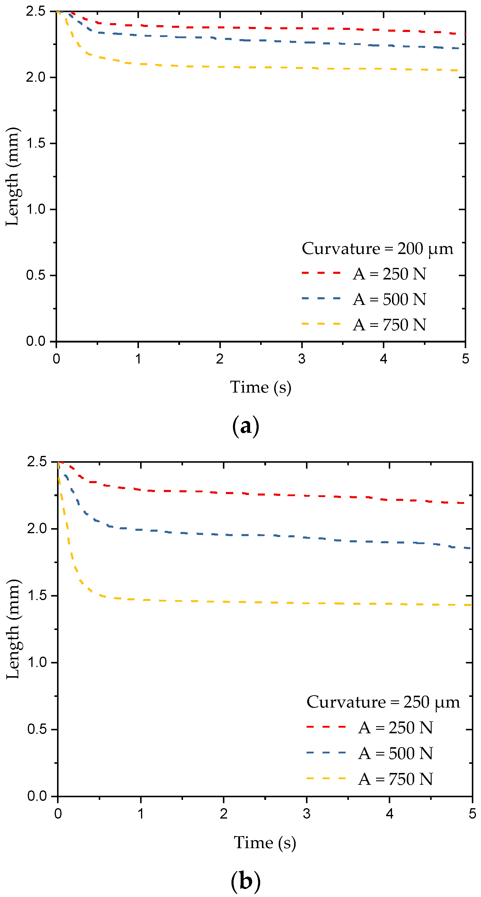As two fibers approach each other, the force increases until it reaches the maximum excluded volume force, which is determined by the value of constant $A$ in Equation (14). Thus, the influence of excluded volume force on fiber length reduction becomes more significant with a higher critical breaking curvature. 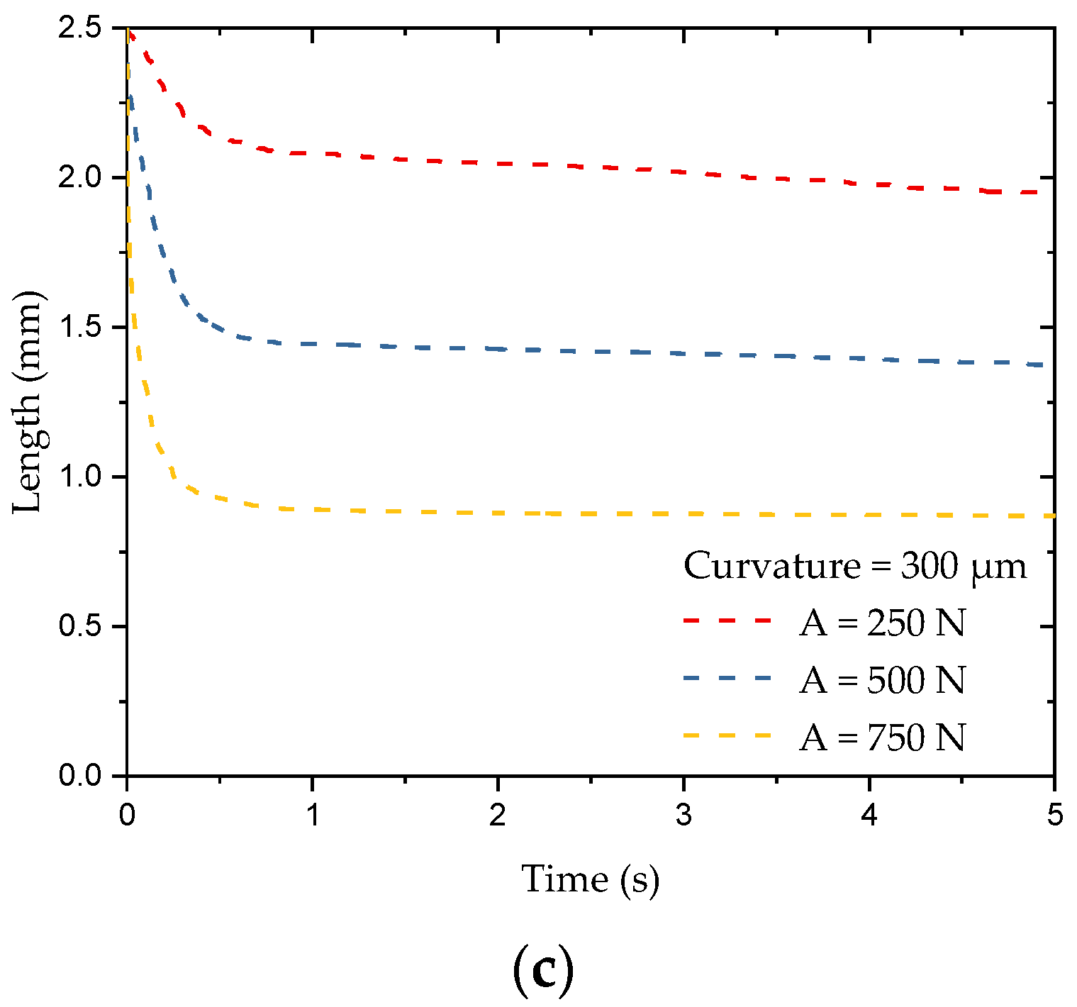This trend can be seen in Figure 8, where the excluded volume force constant varies from 250 to 750, while breaking curvature is the same.

5. Fiber Relaxation

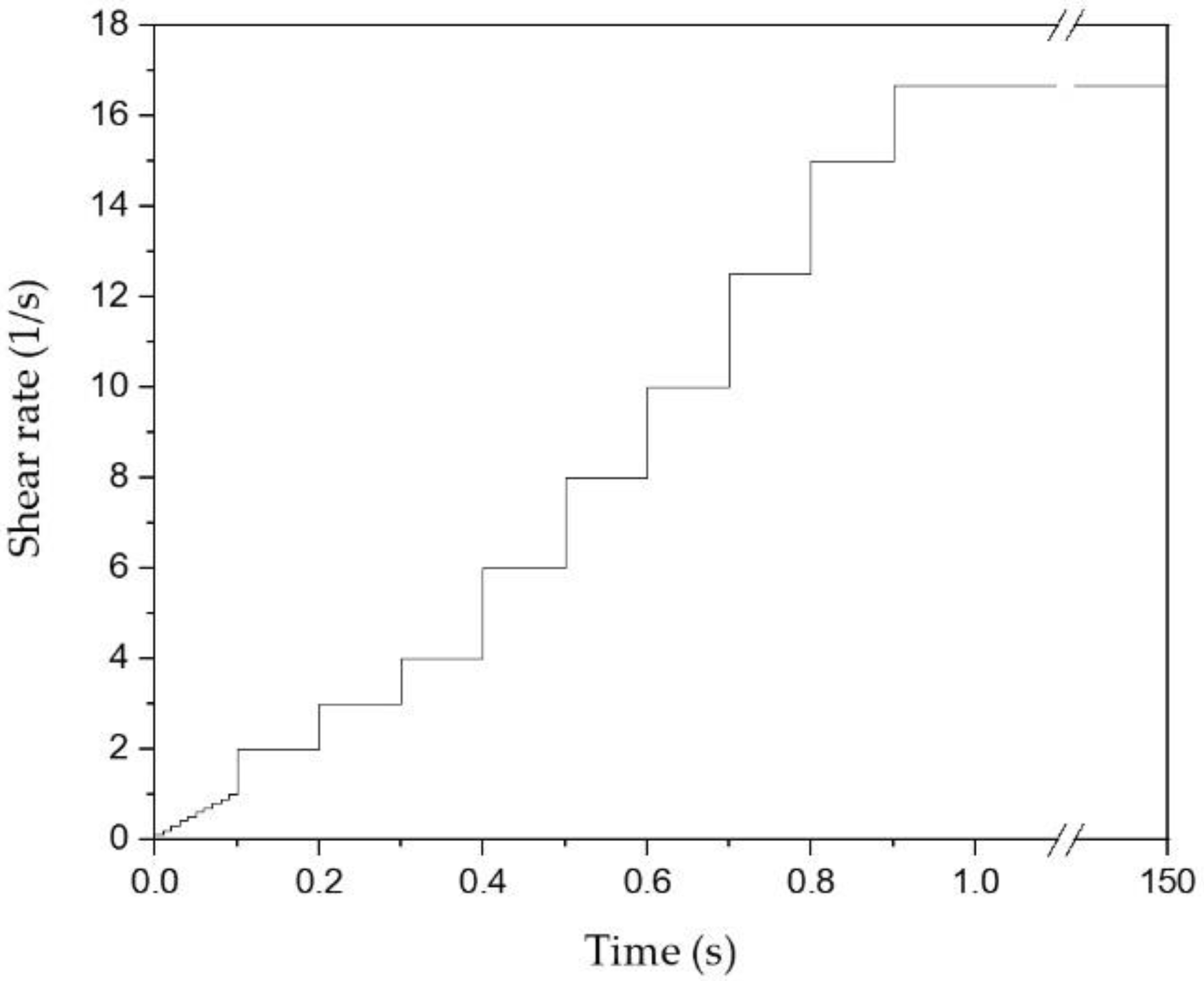
As discussed above, fibers experience a higher breaking rate than those in the experimental results. In order to place thousands of fibers within a small cell, fibers are forced into position with a critical angle, which leads to entanglement and bending of the fibers within the cluster. This entanglement was a big issue during breakage prediction, and can cause overestimation of breakage in the early stage of the simulation. To achieve relaxation of the entanglements, the shear rate was not stepped up instantaneously, but rather, increased in a stepwise fashion from 0 to 16.65 s⁻¹, which is same as the experiment within the first second of simulation time. This allows relaxation of the bent fibers inside the cluster. The simulation shear rate remained at 16.65 s⁻¹ for the remaining 149 s (Figure 9). This technique allowed fibers to straighten out and thus reduce the number of critical angles between the connecting joints, without leading to excessive and unrealistic fiber attrition at the beginning of the simulation.

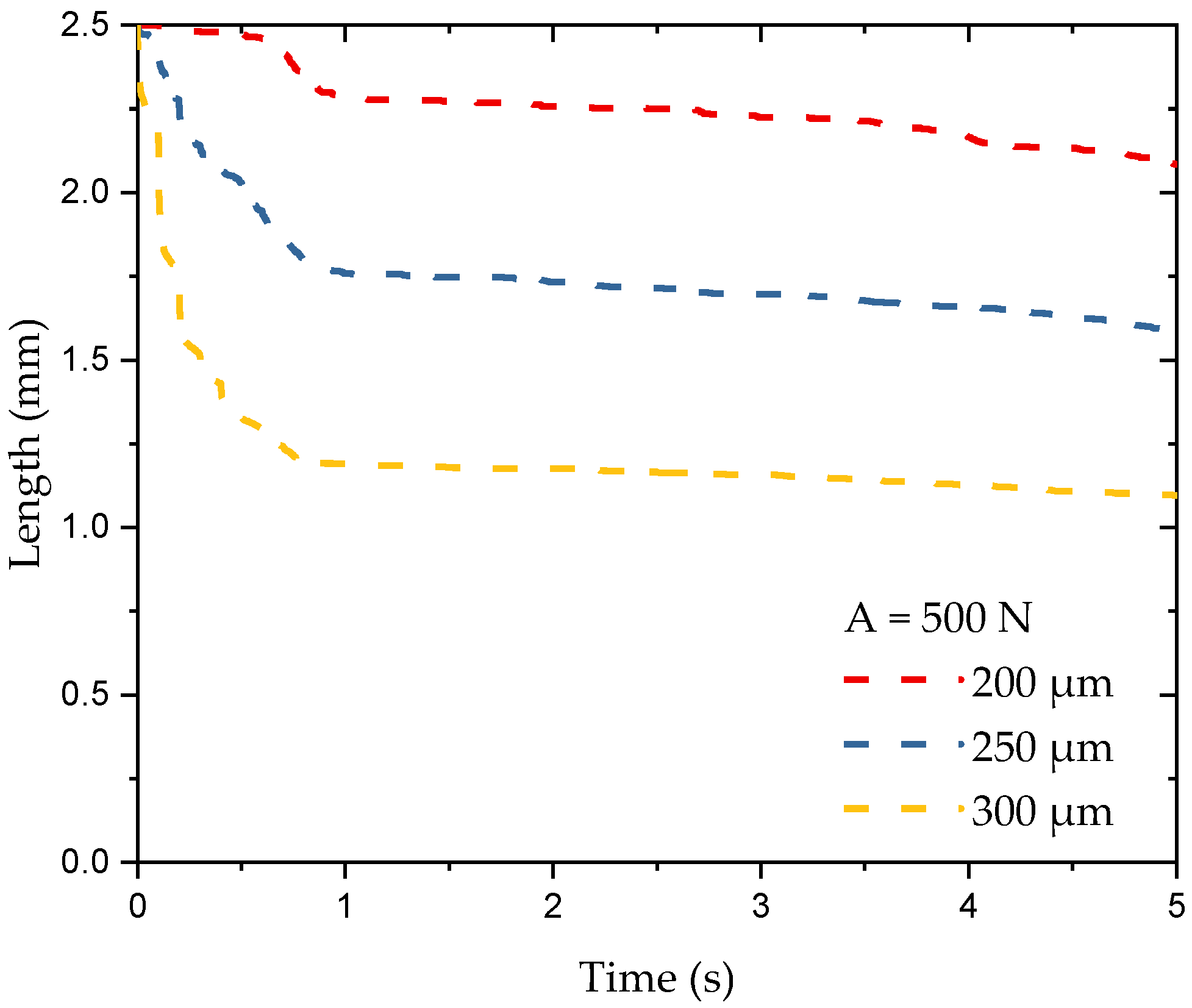
To assess the effect of this relaxation at acceptable computational costs, a relaxation test with a 1 s increase profile was done by tuning critical curvature from 200 $\mathsf{\mu }\mathrm{m}$ to 300 $\mathsf{\mu }\mathrm{m}$ while keeping the force constant $A$ equal to 500 (see Figure 10). Relaxation in the first second of the simulation significantly reduced the initial fiber breakage caused by entanglement during cluster generation, compared to Figure 7b. After the first second, the interaction with neighboring fibers caused by the flow field leads to decreases in fiber curvature, which results in breakage when the assigned critical curvature is reached.

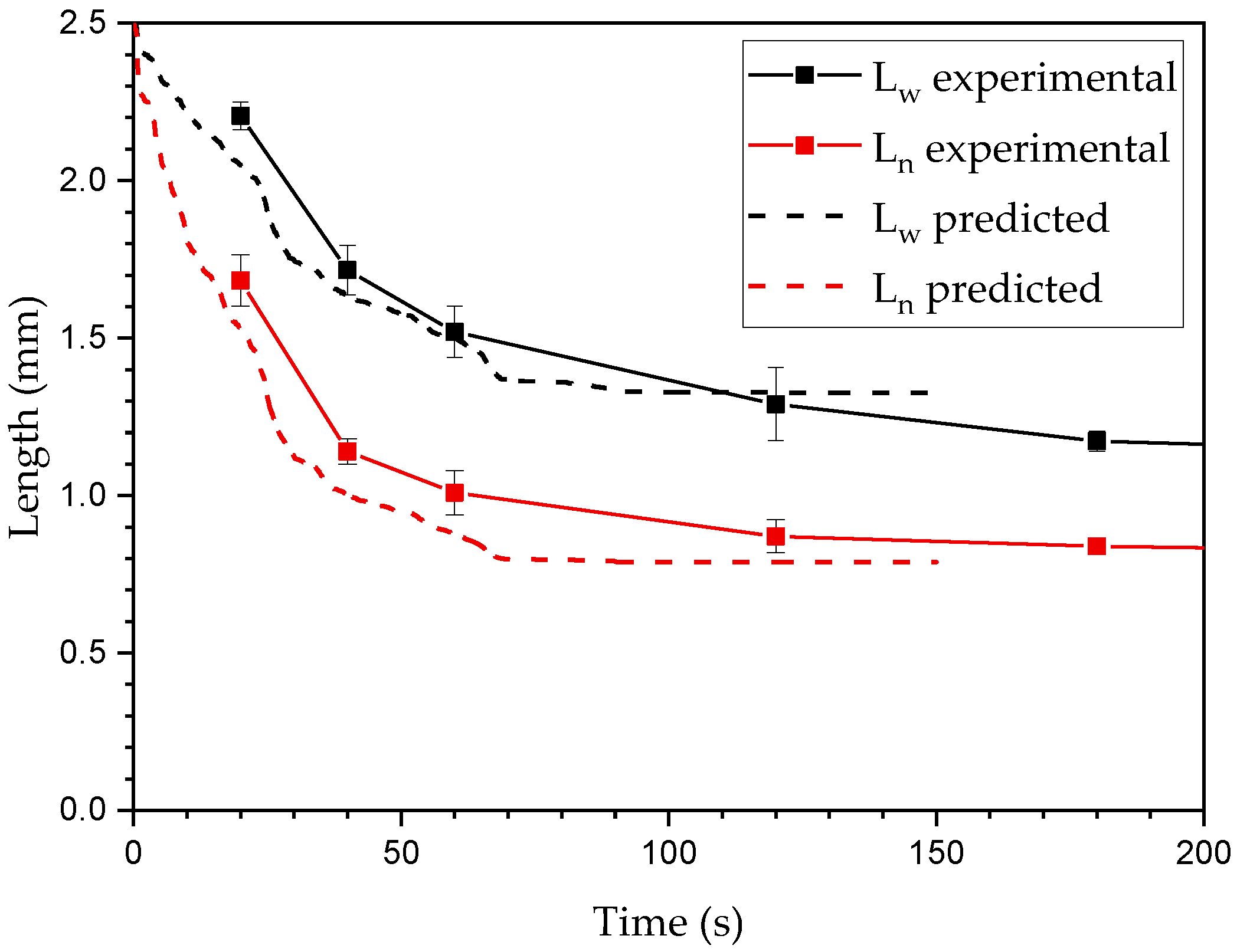
Figure 11 presents a comparison between the Couette experiment and the simulation for a critical curvature of 200 $\mathsf{\mu }\mathrm{m}$ and an excluded volume constant $A$ of 500, with a shear rate increase from 0 to 16.65 s⁻¹ within the first second and remaining at 16.65 throughout the rest of the simulation. As seen in Figure 11, the initial breakage caused by unsteady system is reduced significantly. The simulation matches the experimental results much better. However, there is a slightly faster reduction rate for both $L_n$ and $L_w$, as well as a higher final unbreakable length.

6. Fiber Probability Breakage

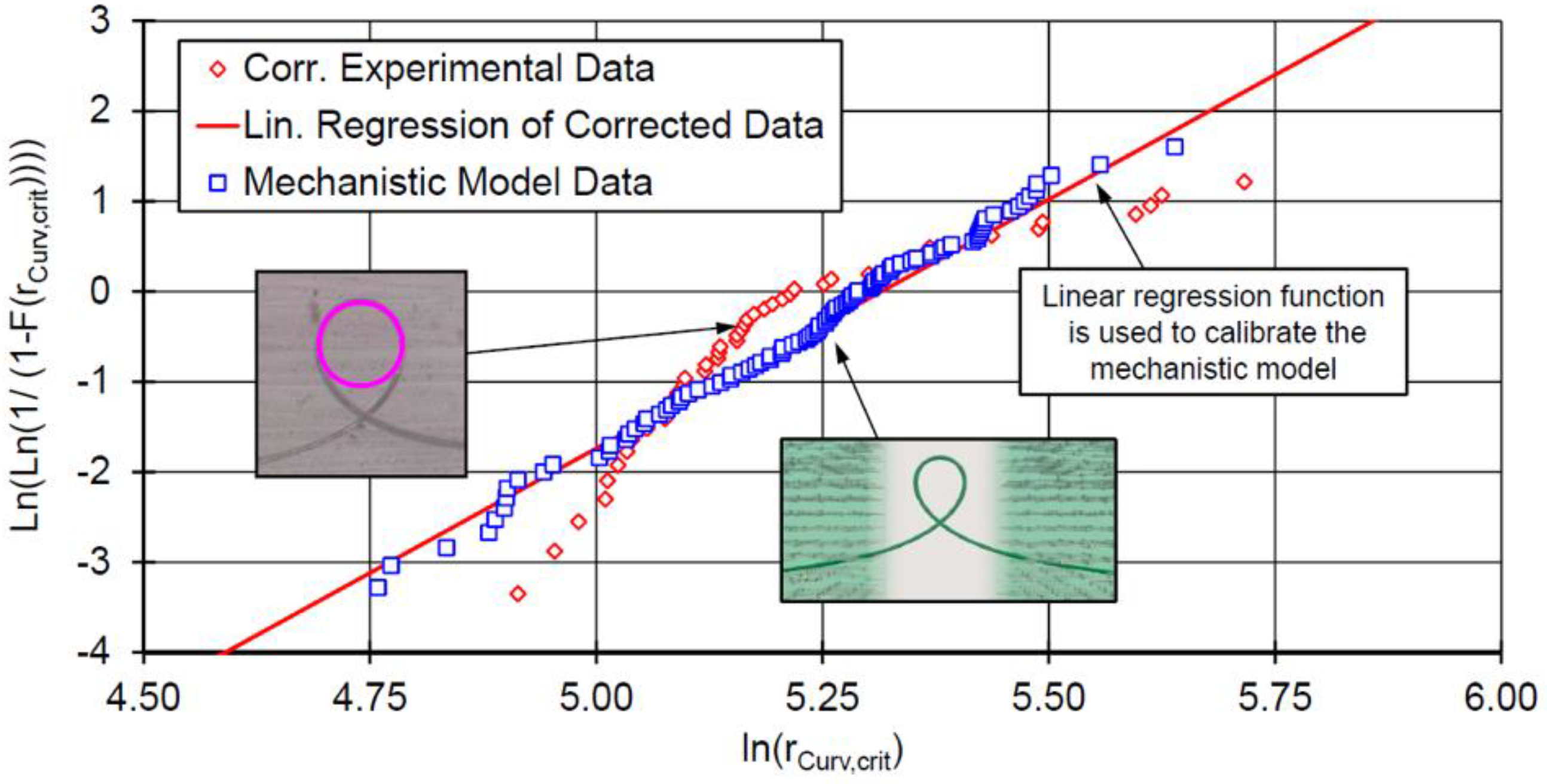
The final part of the fiber attrition model is to introduce the fiber probability measurements. Using the Weibull probability plot (WPP), the mechanistic model was first extended so that the empirically determined fracture behavior of the fibers can be simulated and validated [28]. In Figure 12, the corrected experimental data, calibration curve, and data generated with the mechanistic model are presented in a WPP.

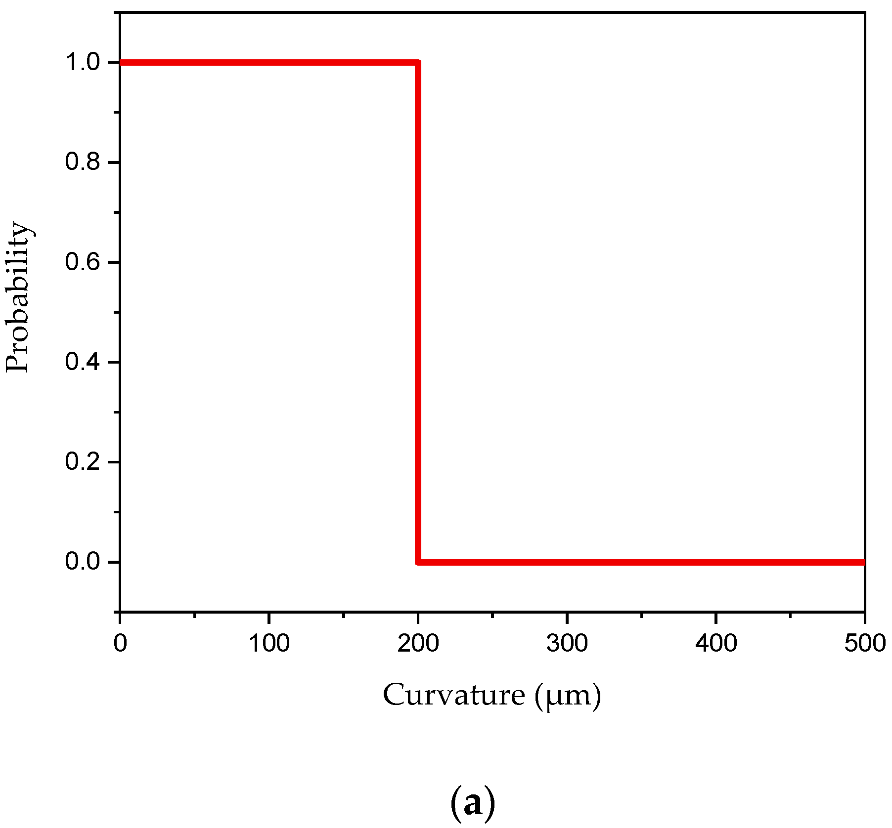
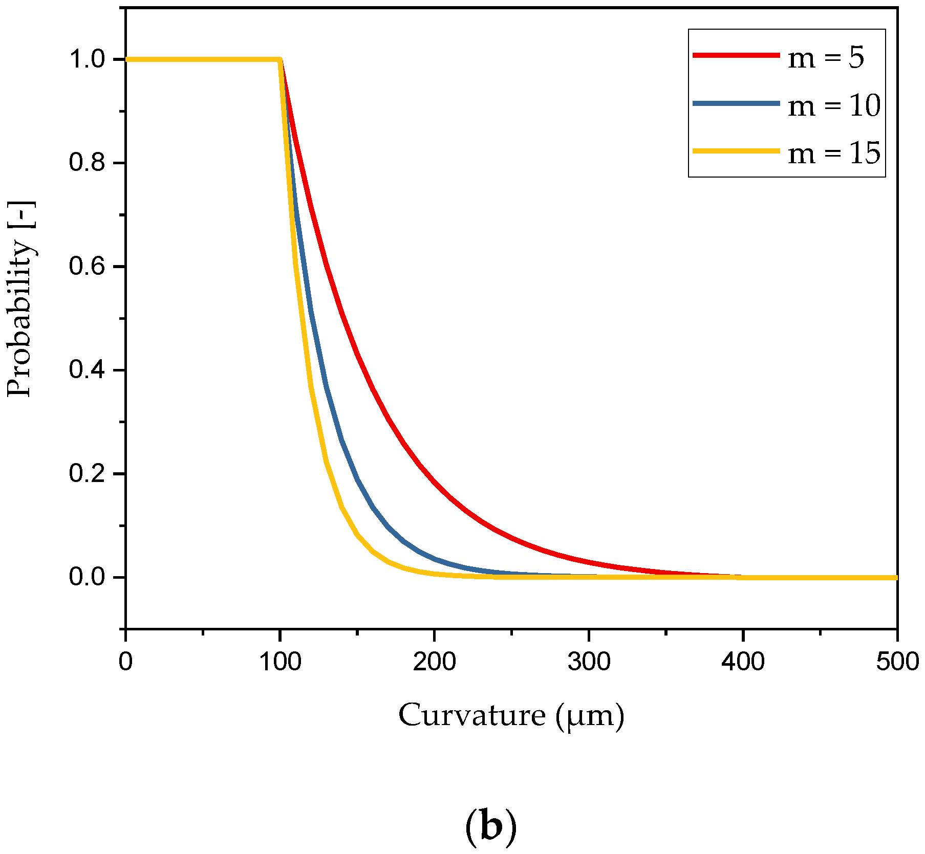
First, it should be noted that linear regression cannot accurately represent experimental data. Consequently, the parameter determination leads to a loss of accuracy and the experimental data cannot be replicated precisely. Thus, a probability function was further introduced into the breakage simulation. Figure 13 presents the breakage criteria with (b) and without (a) an experimental probability of failure distribution. Fibers begin to have a probability to break when its curvature is smaller than the maximum curvature, and will break when curvature reaches the minimum curvature (Figure 13b). Comparing to the fixed curvature, probability theory provides powerful tools to explain the breakage behavior as seen below, where $m$ is chosen as 15 for this research (Figure 13b).

$$x=\frac{\max curvature-curvature}{\max curvature-\min curvature}$$

(16)

$$Probability=\frac{exp\left(m\ast x\right)-1}{exp\left(m\right)-1}$$

(17)

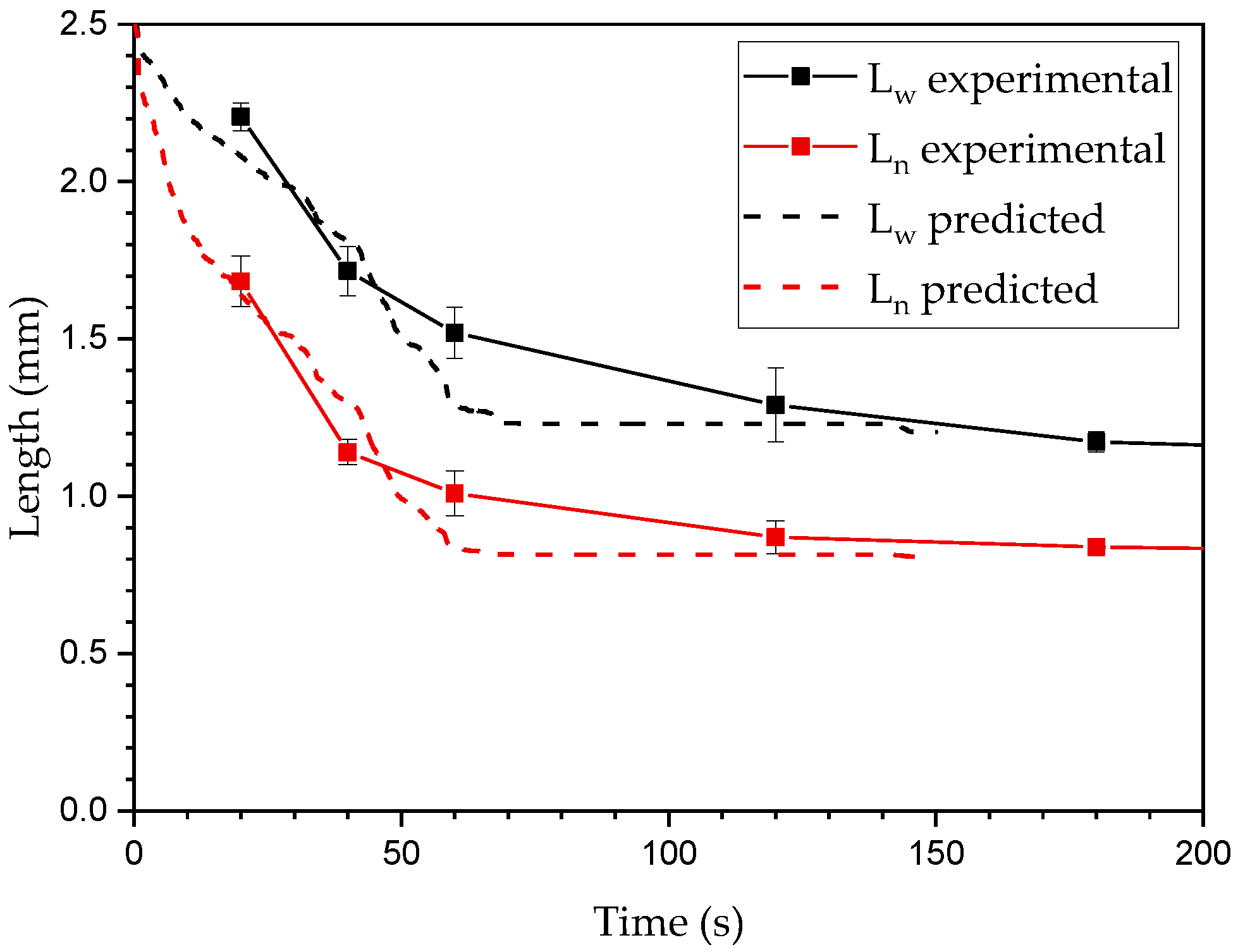
In Figure 14, the model showed a lower initial breakage rate and achieved nearly the experimental steady state fiber length. Unlike the fixed critical breaking curvature, the relaxation allowed fibers to relieve the entanglement and achieve a steady state in the system, which slowed the rate of breakage. As long fibers break into shorter fibers, the chance for fibers to contact each other is reduced, which also results in a higher alignment of fibers in the flow direction. Thus, fibers would gradually align in the flow direction where the rate of breakage significantly reduces after about 60 s. However, due to the Jeffrey orbits, the fibers experience shear flow; if allowing a sufficient amount of time, the fibers eventually rotate and break, which can be seen at around 150 s.

The curvature at break point for Figure 14 was recorded throughout the simulation and shown in Figure 15. Here, only the first 60 s are represented in the distribution, as the length in the simulation remained relatively constant after this period. Compared to Figure 4, which shows the loop experimental result from [28], the predicted distribution showed a similar trend to the experimental data. There was a higher deviation in the range of 200 to 250 $\mathsf{\mu }\mathrm{m}$ and 350 to 400 $\mathsf{\mu }\mathrm{m}$. This may be due to the value of $m$ in Equation (17), selected for this research, being too high for the system. Lowering the value of $m$ will shift the curve to the right (Figure 13b), which increases the probability for fibers to break at a larger curvature. In addition, fiber critical curvature is related to fiber mechanical properties, such as carbon or glass fiber, fiber length, fiber diameter, and Young’s modulus. For example, the minimum critical curvature will be even smaller than the value discussed here for fibers with a lower Young’s modulus.

7. Conclusions and Outlook

A particle level model for computing the breakage behavior for glass fiber in a polypropylene matrix under simple shear flow was studied. The simulation first showed how the variables can be tuned to obtain detailed information about breakage during the processing and develop an understanding of fiber length reduction. Based on the results obtained from the simulation, the length validation on fiber breakage was performed and compared with a Couette flow experiment. However, unsteady initial breakage was observed due to the high fiber volume fraction material used for the experiment. A relaxation of artificial fiber entanglement was introduced to the system. Moreover, a loop test with glass fibers showed a breakage distribution. To better describe breakage behavior, this probability theory was introduced in the simulation. The results had good agreement with the experimental data.

The variations in accuracy of the breakage prediction shows that there is a lack of understanding of the mechanisms involved in the fiber breakage and the respective translation to numerical models. Furthermore, there is not enough experimental data to evaluate the relationship between the excluded volume force and process condition. Thus, future work should conduct relevant experiments and verify the result with mechanistic model simulation to further understand and better describe the effect of excluded volume forces on different systems. Additionally, melting and fiber dispersion effects should be part of future research.