Influence of Failure Criteria and Intralaminar Damage Progression Numerical Models on the Prediction of the Mechanical Behavior of Composite Laminates

Abstract

This work evaluates the effectiveness of commonly adopted local damage evolution methods and failure criteria in finite element analysis for the simulation of intralaminar damage propagation in composites under static loading conditions. The proposed numerical model is based on a User Defined Material subroutine (USERMAT) implemented in Ansys. This model is used to predict the evolution of damage within each specific lamina of a composite laminate by introducing both sudden and gradual degradation rules. The main purpose of the simulations is to quantitatively assess the influence of the adopted failure criteria in conjunction with degradation laws on the accuracy of the numerical predictions in terms of damage evolution and failure load. The mechanical behavior of an open hole tension specimen and of a notched stiffened composite panel under shear loading conditions have been numerically simulated by Progressive Damage Models (PDM). Different failure criteria have been implemented in the developed Ansys USERMAT, together with sudden and gradual degradation rules based on the Continuum Damage Mechanics (CDM) approach. Numerical results have been validated against experimental data to assess the effects of the different failure criteria and damage evolution law on the global mechanical response and local damage predictions in composite laminates.

1. Introduction

The adoption of composite materials for aerospace structures is continuously increasing among industries; however, the methodologies developed so far for the definition of the mechanical response of these materials have not yet achieved a satisfactory level of robustness and reliability. Indeed, the low impact resistance of composites can be very limiting for the effectiveness and weight saving of composite designs. Low velocity impact damage can be very hard to detect, and numerical analyses during the design phase can strongly help in predicting the real impact behavior of composite laminates [1]. Numerical techniques based on Progressive Damage Models (PDM) enable consideration of the presence of an initial damage and stiffness degradation [2]. The degradation of stiffness is usually evaluated at element and lamina level [3]. Furthermore, the material degradation models are called “instantaneous” where the properties are suddenly degraded, and “gradual” [4] when the properties are gradually degraded, according to linear or exponential laws.

The onset of the damage mechanisms in composites, in a Progressive Damage Model, is evaluated by adopting proper failure criteria. Failure criteria can be split into two general groups: non-interactive criteria and interactive criteria [5]. Maximum stress and strain criteria do not include interaction between stress components to estimate fiber damage and matrix damage. Interactive failure criteria, on the other hand, use separate expressions to identify fiber and matrix failure under tensile and compression loading conditions. Examples of interactive criteria are the Hashin [6], Chang–Chang [7] and Hou [8] criteria. Puck and Schürmann [9], subsequently, modified the Hashin criteria by introducing a model of a fracture plane for matrix damage to simulate the “low” fracture behavior. Previous studies, e.g., in [10] have compared the effectiveness of damage model and failure criteria. These failure criteria are commonly applied within Progressive Damage Models in industrial Finite Element (FE) codes.

Many examples can be found in literature, e.g., in [11] where the instantaneous methodology in Progressive Damage Models has been implemented using Hashin failure criterion. Other works have improved the reliability of Progressive Damage Models and their use in the numerical approaches [12,13,14], or, e.g., in [15] the damage model has been implemented as code in the FE software. In the present works two numerical test-cases are introduced: an open hole panel under tensile load by Chen at al. [16] and a stiffened panel subjected to static shear loading conditions by Ambur et al. [17]. Experimental data are available from literature for both these numerical models [16,17]. The scope of this paper is to assess how the effectiveness of the numerical model is influenced by the failure criteria and the Progressive Damage Model adopted for simulations.

Starting from the numerical model developed by Riccio et al. in [18], different three-dimensional failure criteria (maximum stress, Hashin, and Puck criteria) and “instantaneous” and “gradual” progressive damage models with suitable degradation rules have been implemented in the Ansys FE code USERMAT. This has been undertaken in order to compare the failure criteria together with Sudden and Gradual Progressive Degradation Models [19]. To assess the influence of the adopted numerical model on the accuracy of the numerical prediction, the numerical results have been compared with literature experimental data for the analyzed test cases.

In Section 2, the theory behind the Sudden and Gradual Progressive Degradation Models is presented. The adopted failure criteria and the Finite Element Method (FEM) implementation in the software ANSYS© as User Defined Material Subroutine (USERMAT) are also described. In Section 3, the two analyzed test-cases are presented together with a mesh convergence study performed for the Open Hole Tensile specimen. Finally, in Section 4, the results in terms of matrix and fiber failure are shown. The experimental literature data [17,20] and the numerical outputs from Sudden and Gradual Degradation Models are compared to assess the reliability of the methods applied for intralaminar damage prediction [21].

2. Theoretical Background and Finite Element Implementation

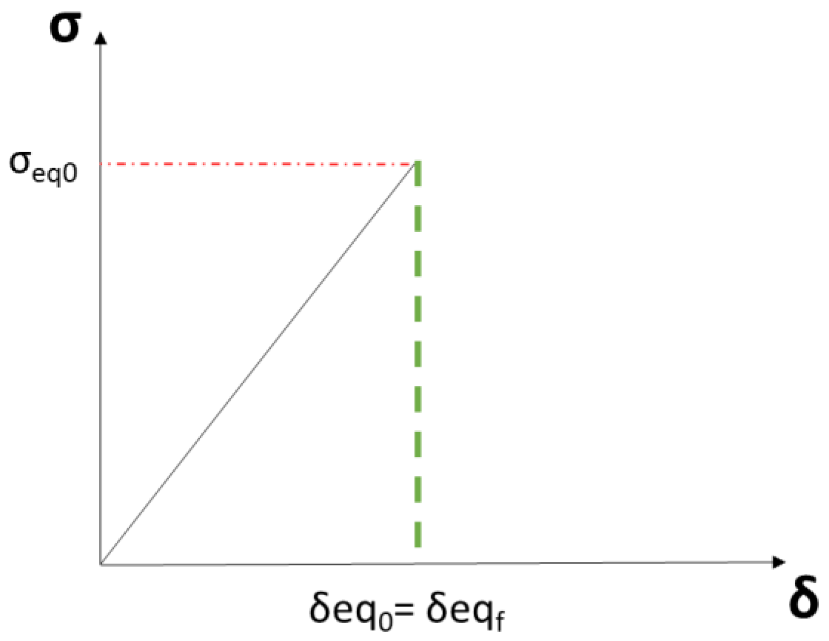
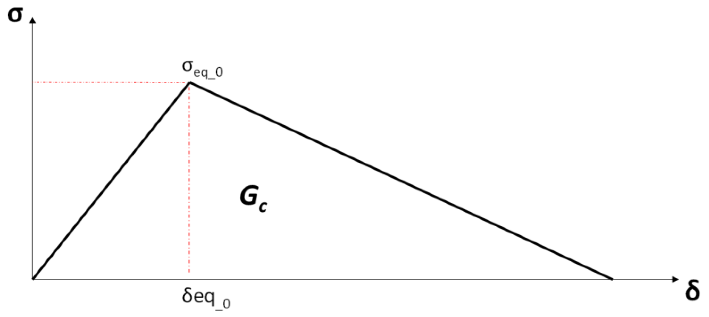
2.1. Progressive Damage Models

The intralaminar damage models implemented are based on the following assumptions: the damage process is supposed to take place in one finite element at a time, internal damage variables ${\mathit{d}}_{\mathit{i}\mathit{j}}$, assembled in a damage matrix $\mathit{D}$, are introduced to measure damage extent and stiffness degradation associated to specific fiber or matrix damage mode, stress-strain based initiation criteria and fracture energy-based evolution laws are defined for each specific failure mode. Each of damage parameters ${\mathit{d}}_{\mathit{i}\mathit{j}}$ is a component of the damage matrix $\mathit{D}$ associated to a specific component of the undamaged stress tensor $\overline{\mathbf{\sigma }}$ (effective stress tensor), which can be related to the true stress tensor σ by the following relation:

$$\mathbf{\sigma }=\mathit{D}\overline{\mathbf{\sigma }}=\mathit{D}\mathit{E}\mathbf{\epsilon }$$

(1)

where $\mathit{D}$ indicates the undamaged material stiffness matrix. The behavior of the material at a specific location, during its degradation, is correlated to the stress/strain at that location. In particular, when considering “gradual” degradation laws, the material behavior is first assumed as linear up to the damage onset; then, in the degradation phase, a linear of parabolic constitutive law is considered. In the degradation phase, the original undamaged stiffness matrix of the material is replaced by a new matrix known as the damaged stiffness matrix [22].

$$\left[{\mathit{C}}_{\mathit{d}}\right]=\left[\begin{array}{cccccc}{\mathit{C}}_{\mathbf{11}}& {\mathit{C}}_{\mathbf{12}}& {\mathit{C}}_{\mathbf{13}}& \mathbf{0}& \mathbf{0}& \mathbf{0}\\ {\mathit{C}}_{\mathbf{12}}& {\mathit{C}}_{\mathbf{22}}& {\mathit{C}}_{\mathbf{23}}& \mathbf{0}& \mathbf{0}& \mathbf{0}\\ {\mathit{C}}_{\mathbf{13}}& {\mathit{C}}_{\mathbf{23}}& {\mathit{C}}_{\mathbf{33}}& \mathbf{0}& \mathbf{0}& \mathbf{0}\\ \mathbf{0}& \mathbf{0}& \mathbf{0}& {\mathit{C}}_{\mathbf{44}}& \mathbf{0}& \mathbf{0}\\ \mathbf{0}& \mathbf{0}& \mathbf{0}& \mathbf{0}& {\mathit{C}}_{\mathbf{55}}& \mathbf{0}\\ \mathbf{0}& \mathbf{0}& \mathbf{0}& \mathbf{0}& \mathbf{0}& {\mathit{C}}_{\mathbf{66}}\end{array}\right]$$

(2)

With

$${\mathit{C}}_{\mathbf{11}}=\frac{{\mathit{E}}_{\mathbf{1}}{}^{\mathbf{3}}{\mathit{E}}_{\mathbf{2}}\left(\mathbf{1}-{\mathit{d}}_{\mathit{f}}\right)\left({\mathit{E}}_{\mathbf{2}}-{\mathit{E}}_{\mathbf{3}}{\left(\mathbf{1}-{\mathit{d}}_{\mathit{m}}\right)}^{\mathbf{2}}{\mathbf{\nu }}_{\mathbf{13}}{}^{\mathbf{2}}\right)}{\mathit{A}}$$

(3)

$${\mathit{C}}_{\mathbf{22}}=\frac{{\mathit{E}}_{\mathbf{1}}{\mathit{E}}_{\mathbf{2}}{}^{\mathbf{3}}\left(\mathbf{1}-{\mathit{d}}_{\mathit{m}}\right)\left({\mathit{E}}_{\mathbf{1}}-{\mathit{E}}_{\mathbf{3}}\left(\mathbf{1}-{\mathit{d}}_{\mathit{m}}\right)\left(\mathbf{1}-{\mathit{d}}_{\mathit{f}}\right){\mathbf{\nu }}_{\mathbf{13}}{}^{\mathbf{2}}\right)}{\mathit{A}}$$

(4)

$${\mathit{C}}_{\mathbf{33}}=\frac{{\mathit{E}}_{\mathbf{1}}{\mathit{E}}_{\mathbf{2}}{}^{\mathbf{2}}{\mathit{E}}_{\mathbf{1}}\left(\mathbf{1}-{\mathit{d}}_{\mathit{m}}\right)\left({\mathit{E}}_{\mathbf{1}}-{\mathit{E}}_{\mathbf{2}}\left(\mathbf{1}-{\mathit{d}}_{\mathit{f}}\right)\left(\mathbf{1}-{\mathit{d}}_{\mathit{m}}\right){\mathbf{\nu }}_{\mathbf{12}}{}^{\mathbf{2}}\right)}{\mathit{A}}$$

(5)

$${\mathit{C}}_{\mathbf{12}}=\frac{{\mathit{E}}_{\mathbf{1}}{}^{\mathbf{2}}{\mathit{E}}_{\mathbf{2}}{}^{\mathbf{2}}\left(\mathbf{1}-{\mathit{d}}_{\mathit{f}}\right)\left(\mathbf{1}-{\mathit{d}}_{\mathit{m}}\right)\left({\mathit{E}}_{\mathbf{2}}{\mathbf{\nu }}_{\mathbf{12}}-{\mathit{E}}_{\mathbf{3}}\left(\mathbf{1}-{\mathit{d}}_{\mathit{m}}\right){\mathbf{\nu }}_{\mathbf{13}}{\mathbf{\nu }}_{\mathbf{23}}\right)}{\mathit{A}}$$

(6)

$${\mathit{C}}_{\mathbf{13}}=\frac{{\mathit{E}}_{\mathbf{1}}{}^{\mathbf{2}}{\mathit{E}}_{\mathbf{2}}{\mathit{E}}_{\mathbf{3}}\left(\mathbf{1}-{\mathit{d}}_{\mathit{f}}\right)\left(\mathbf{1}-{\mathit{d}}_{\mathit{m}}\right)\left({\mathit{E}}_{\mathbf{2}}{\mathbf{\nu }}_{\mathbf{13}}+{\mathit{E}}_{\mathbf{2}}\left(\mathbf{1}-{\mathit{d}}_{\mathit{m}}\right){\mathbf{\nu }}_{\mathbf{12}}{\mathbf{\nu }}_{\mathbf{23}}\right)}{\mathit{A}}$$

(7)

$${\mathit{C}}_{\mathbf{23}}=\frac{{\mathit{E}}_{\mathbf{2}}{}^{\mathbf{2}}{\mathit{E}}_{\mathbf{1}}{\mathit{E}}_{\mathbf{3}}{\left(\mathbf{1}-{\mathit{d}}_{\mathit{m}}\right)}^{\mathbf{2}}\left({\mathit{E}}_{\mathbf{1}}{\mathbf{\nu }}_{\mathbf{23}}+{\mathit{E}}_{\mathbf{2}}\left(\mathbf{1}-{\mathit{d}}_{\mathit{f}}\right){\mathbf{\nu }}_{\mathbf{12}}{\mathbf{\nu }}_{\mathbf{23}}\right)}{\mathit{A}}$$

(8)

$${\mathit{C}}_{\mathbf{44}}={\mathit{G}}_{\mathbf{12}}\left(\mathbf{1}-{\mathit{d}}_{\mathit{s}}\right)\hspace{1em}\hspace{1em}{\mathit{C}}_{\mathbf{55}}={\mathit{G}}_{\mathbf{23}}\left(\mathbf{1}-{\mathit{d}}_{\mathit{s}}\right)\hspace{1em}\hspace{1em}{\mathit{C}}_{\mathbf{66}}={\mathit{G}}_{\mathbf{13}}\left(1-{\mathit{d}}_{\mathit{s}}\right)$$

(9)

where

$$\begin{gathered} \mathit{A}={\mathit{E}}_{\mathbf{1}}{}^{\mathbf{2}}{\mathit{E}}_{\mathbf{2}}{}^{\mathbf{2}}\left(\mathbf{1}-\left(\mathbf{1}-{\mathit{d}}_{\mathit{f}}\right)\left(\mathbf{1}-{\mathit{d}}_{\mathit{m}}\right){\mathbf{\nu }}_{\mathbf{12}}{\mathbf{\nu }}_{\mathbf{21}}-\left(\mathbf{1}-{\mathit{d}}_{\mathit{f}}\right)\left(\mathbf{1}-{\mathit{d}}_{\mathit{m}}\right){\mathbf{\nu }}_{\mathbf{13}}{\mathbf{\nu }}_{\mathbf{31}}- \\ {\left(\mathbf{1}-{\mathit{d}}_{\mathit{m}}\right)}^{\mathbf{2}}{\mathbf{\nu }}_{\mathbf{32}}{\mathbf{\nu }}_{\mathbf{23}}-\mathbf{2}\left(\mathbf{1}-{\mathit{d}}_{\mathit{f}}\right){\left(\mathbf{1}-{\mathit{d}}_{\mathit{m}}\right)}^{\mathbf{2}}{\mathbf{\nu }}_{\mathbf{31}}{\mathbf{\nu }}_{\mathbf{23}}{\mathbf{\nu }}_{\mathbf{12}}\right) \end{gathered}$$

(10)

${\mathit{d}}_{\mathit{f}}$, ${\mathit{d}}_{\mathit{m}}$ and ${\mathit{d}}_{\mathit{s}}$ are, respectively, damage variables for fiber, matrix, and shear damage. These damage variables can depend on the compression or tension loading modes. Hence, the damage variables ${\mathit{d}}_{\mathit{f}\mathit{t}}$, ${\mathit{d}}_{\mathit{f}\mathit{c}}$, ${\mathit{d}}_{\mathit{m}\mathit{t}}$ and ${\mathit{d}}_{\mathit{m}\mathit{c}}$ correlating to distinct failure modes (fiber failure related to tension and compression, matrix failure—tension and compression) can be introduced. The following relations hold:

$${\mathit{d}}_{\mathit{f}}=\{\begin{array}{c}{\mathit{d}}_{\mathit{f}\mathit{t}}\hspace{1em}\hspace{1em}{\mathbf{\sigma }}_{\mathbf{1}}\ge \mathbf{0}\hspace{1em}\hspace{1em}\\ {\mathit{d}}_{\mathit{f}\mathit{c}\hspace{1em}\hspace{1em}} {\mathbf{\sigma }}_{\mathbf{1}}<\mathbf{0}\hspace{1em}\hspace{1em}\end{array}\hspace{1em}\hspace{1em}{\mathit{d}}_{\mathit{m}}=\{\begin{array}{c}{\mathit{d}}_{\mathit{m}\mathit{t}}\hspace{1em}\hspace{1em}{\mathbf{\sigma }}_{\mathbf{2}}\ge \mathbf{0} \\ {\mathit{d}}_{\mathit{m}\mathit{c}}\hspace{1em}\hspace{1em}{\mathbf{\sigma }}_{\mathbf{2}}<\mathbf{0}\end{array}$$

(11)

$${\mathit{d}}_{\mathit{s}}=\mathbf{1}-\left(\mathbf{1}-{\mathit{d}}_{\mathit{f}\mathit{t}}\right)\left(\mathbf{1}-{\mathit{d}}_{\mathit{f}\mathit{c} }\right)\left(\mathbf{1}-{\mathit{d}}_{\mathit{m}\mathit{t}}\right)\left(\mathbf{1}-{\mathit{d}}_{\mathit{m}\mathit{c}}\right)$$

(12)

The damage variables range from 0 (undamaged status) to 1 (complete damage status). The strength criteria are evaluated according to the effective stress, $\tilde{\mathbf{\sigma }}$. $\tilde{\mathbf{\sigma }}$ can be derived from the nominal stress by using a damage operator, [$M$]. The relation between the effective stress $\tilde{\mathbf{\sigma }}$ and the nominal stress σ can be written as:

$$\widetilde{\left\{\mathbf{\sigma }\right\}}=\left[M\right]\left\{\mathbf{\sigma }\right\}$$

(13)

$$\mathrm{where} [M]=\left[\begin{array}{cccccc}\frac{\mathbf{1}}{\left(\mathbf{1}-{\mathit{d}}_{\mathit{f}}\right)}& & & & & \\ & \frac{\mathbf{1}}{\left(\mathbf{1}-{\mathit{d}}_{\mathit{f}}\right)}& & & & \\ & & \frac{\mathbf{1}}{\left(\mathbf{1}-{\mathit{d}}_{\mathit{m}}\right)}& & & \\ & & & \frac{\mathbf{1}}{\left(\mathbf{1}-{\mathit{d}}_{\mathit{s}}\right)}& & \\ & & & & \frac{\mathbf{1}}{\left(\mathbf{1}-{\mathit{d}}_{\mathit{s}}\right)}& \\ & & & & & \frac{\mathbf{1}}{\left(\mathbf{1}-{\mathit{d}}_{\mathit{s}}\right)}\end{array}\right]$$

(14)

Complete failure is reached in a localized area at the end of the softening phase where the deformation is the maximum possible. This approach is mesh dependent because the dissipated energy reduces for increased mesh refinements.

In order to reduce effects related to mesh dependence, the equivalent strain and stress can be introduced. These quantities, according to each damage mode, can be formulated in terms of effective strain and stress components as:

• Fiber tension failure (${\tilde{\mathbf{\sigma }}}_{\mathbf{11}}\ge \mathbf{0})$

  $${\mathbf{\epsilon }}_{\mathit{f}\mathit{t},\mathit{e}\mathit{q}}^{}=\sqrt{⟨{\mathbf{\epsilon }}_{\mathbf{11}}⟩{}^{\mathbf{2}}+{\mathbf{\gamma }}_{\mathbf{12}}{}^{\mathbf{2}}+{\mathbf{\gamma }}_{\mathbf{13}}{}^{\mathbf{2}}}$$

  (15)

  $${\mathbf{\sigma }}_{\mathit{f}\mathit{t},\mathit{e}\mathit{q}}^{}=\frac{⟨{\mathbf{\sigma }}_{\mathbf{11}}⟩⟨{\mathbf{\epsilon }}_{\mathbf{11}}⟩+{\mathbf{\tau }}_{\mathbf{13}}{\mathbf{\gamma }}_{\mathbf{13}}}{{\mathbf{\epsilon }}_{\mathit{e}\mathit{q}}^{\mathit{f}\mathit{t}}}$$

  (16)
• Fiber compression failure (${\tilde{\mathbf{\sigma }}}_{\mathbf{11}}<\mathbf{0})$

  $${\mathbf{\epsilon }}_{\mathit{f}\mathit{c},\mathit{e}\mathit{q}}^{}=-⟨{\mathbf{\epsilon }}_{\mathbf{11}}⟩$$

  (17)

  $${\mathbf{\sigma }}_{\mathit{f}\mathit{c},\mathit{e}\mathit{q}}^{}=\frac{-⟨{\mathbf{\sigma }}_{11}⟩⟨{\mathbf{\epsilon }}_{11}⟩}{{\mathbf{\epsilon }}_{\mathit{e}\mathit{q}}^{\mathit{f}\mathit{c}}}$$

  (18)
• Matrix tension failure (${\tilde{\mathbf{\sigma }}}_{\mathbf{22}}\ge \mathbf{0})$

  $${\mathbf{\epsilon }}_{\mathit{m}\mathit{t},\mathit{e}\mathit{q}}^{}=\sqrt{⟨{\mathbf{\epsilon }}_{\mathbf{22}}⟩{}^{\mathbf{2}}+⟨{\mathbf{\epsilon }}_{\mathbf{33}}⟩{}^{\mathbf{2}}+{\mathbf{\gamma }}_{\mathbf{12}}{}^{\mathbf{2}}+{\mathbf{\gamma }}_{\mathbf{23}}{}^{\mathbf{2}}+{\mathbf{\gamma }}_{\mathbf{13}}{}^{\mathbf{2}}}$$

  (19)

  $${\mathbf{\sigma }}_{\mathit{m}\mathit{t},\mathit{e}\mathit{q}}^{}=\frac{⟨{\mathbf{\sigma }}_{\mathbf{22}}⟩⟨{\mathbf{\epsilon }}_{\mathbf{22}}⟩+⟨{\mathbf{\sigma }}_{\mathbf{33}}⟩⟨{\mathbf{\epsilon }}_{\mathbf{33}}⟩+{\mathbf{\tau }}_{\mathbf{12}}{\mathbf{\gamma }}_{\mathbf{12}}+{\mathbf{\tau }}_{\mathbf{23}}{\mathbf{\gamma }}_{\mathbf{23}}+{\mathbf{\tau }}_{\mathbf{13}}{\mathbf{\gamma }}_{\mathbf{13}}}{{\mathbf{\epsilon }}_{\mathit{e}\mathit{q}}^{\mathit{m}\mathit{t}}}$$

  (20)
• Matrix compression failure (${\tilde{\mathbf{\sigma }}}_{\mathbf{22}}<\mathbf{0})$

  $${\mathbf{\epsilon }}_{\mathit{m}\mathit{c},\mathit{e}\mathit{q}}^{}=\sqrt{⟨-{\mathbf{\epsilon }}_{\mathbf{22}}⟩{}^{\mathbf{2}}+⟨-{\mathbf{\epsilon }}_{\mathbf{33}}⟩{}^{\mathbf{2}}+{\mathbf{\gamma }}_{\mathbf{12}}{}^{\mathbf{2}}+{\mathbf{\gamma }}_{\mathbf{23}}{}^{\mathbf{2}}+{\mathbf{\gamma }}_{\mathbf{13}}{}^{\mathbf{2}}}$$

  (21)

  $${\mathbf{\sigma }}_{\mathit{m}\mathit{c},\mathit{e}\mathit{q}}^{}=\frac{⟨-{\mathbf{\sigma }}_{\mathbf{22}}⟩⟨-{\mathbf{\epsilon }}_{\mathbf{22}}⟩+⟨-{\mathbf{\sigma }}_{\mathbf{33}}⟩⟨-{\mathbf{\epsilon }}_{\mathbf{33}}⟩+{\mathbf{\tau }}_{\mathbf{12}}{\mathbf{\gamma }}_{\mathbf{12}}+{\mathbf{\tau }}_{\mathbf{23}}{\mathbf{\gamma }}_{\mathbf{23}}+{\mathbf{\tau }}_{\mathbf{13}}{\mathbf{\gamma }}_{\mathbf{13}}}{{\mathbf{\epsilon }}_{\mathit{e}\mathit{q}}^{\mathit{m}\mathit{c}}}$$

  (22)

  where the symbol, 〈〉, denotes the Macaulay Operator, defined ∀ω∈ℜ, as 〈ω〉 = (ω+|ω|)/2.

The equivalent displacements can be found from the resulting relation:

$${\mathbf{\delta }}_{\mathit{i},\mathit{e}\mathit{q}}={\mathit{L}}_{\mathit{c}}{\mathbf{\epsilon }}_{\mathit{i},\mathit{e}\mathit{q}}\hspace{1em}\hspace{1em}\mathit{i}\in \left\{{\mathit{f}}_{\mathit{t}},{\mathit{f}}_{\mathit{c}},{\mathit{m}}_{\mathit{t}},{\mathit{m}}_{\mathit{c}}\right\}$$

(23)

The final failure equivalent displacement ${\mathbf{\delta }}_{\mathit{f},\mathit{i},\mathit{e}\mathit{q}}$ for each failure mode is evaluated as a multiple of the equivalent displacement at failure initiation ${\mathbf{\delta }}_{\mathbf{0},,\mathit{i},\mathit{e}\mathit{q}}$ which is given by the following relation:

$${\mathbf{\delta }}_{\mathbf{0},\mathit{i},\mathit{e}\mathit{q}}={\mathit{L}}_{\mathit{c}}{\mathbf{\epsilon }}_{\mathbf{0},\mathit{i},\mathit{e}\mathit{q}}$$

(24)

where ${\mathbf{\epsilon }}_{\mathbf{0},\mathit{i},\mathit{E}\mathit{q}}$ is the equivalent strain at failure initiation for the failure mode $\mathit{i}$, ${\mathit{L}}_{\mathit{c}}$ is the characteristic length introduced to normalize the element volume and remove the mesh dependency.

This progressive degradation model can be applied for “sudden” and “gradual” degradation.

According to the Sudden Degradation Model, all material properties are instantaneously reduced. In reality, the properties are degraded to a small fraction of the undamaged properties.

In Figure 1, the concept of sudden degradation is schematized. ${\mathbf{\sigma }}_{\mathit{e}\mathit{q}\mathbf{0}}$ is the initial equivalent stress and the ${\mathbf{\delta }}_{\mathit{e}\mathit{q}\mathbf{0}}$ is the initial equivalent displacement which, in sudden degradation, is equal to the final equivalent displacement ${\mathbf{\delta }}_{\mathit{e}\mathit{q}\mathit{f}}$.

On the other hand, in gradual degradation models, the evolution and damage accumulation for each failure mode is represented by a gradual degradation of material properties. This requires parameters that are able to follow the damage evolution. A sample bilinear law representing gradual damage evolution is schematically represented in Figure 2.

In Figure 2, the area of triangle ${\mathit{G}}_{\mathit{c}}$, is the critical energy value, which is a material characteristic.

The final equivalent displacement satisfying the comparison between the dissipated energy and the intralaminar fracture energy ${\mathit{G}}_{\mathit{I}}{}^{\mathit{C}}$ (for the I-th fracture mode) can be found from the relation:

$${\mathit{G}}_{\mathit{I}}{}^{\mathit{C}}=\frac{\mathbf{1}}{\mathbf{2}}{\mathbf{\sigma }}_{\mathit{I},\mathit{e}\mathit{q}}^{\mathbf{0}}{\mathbf{\delta }}_{\mathit{e}\mathit{q}}^{\mathit{f}}\to {\mathbf{\delta }}_{\mathit{I},\mathit{e}\mathit{q}}^f=\frac{\mathbf{2}{\mathit{G}}_{\mathit{I}}{}^{\mathit{C}}}{{\mathbf{\sigma }}_{\mathit{i},\mathit{e}\mathit{q}}^{\mathbf{0}}}$$

(25)

where ${\mathit{G}}_{\mathit{I}}{}^{\mathit{C}}$ is the intralaminar fracture energy of the material for failure mode I. The equivalent stress at failure initiation ${\mathbf{\sigma }}_{\mathit{I},\mathit{e}\mathit{q}}^{\mathbf{0}}$, for failure mode I, does not change with element size. The final equivalent displacement value ${\mathbf{\delta }}_{\mathit{I},\mathit{E}\mathit{q}}{}^{\mathit{f}}$ results are also unchanged with the element size. However, the initial failure equivalent displacement ${\mathbf{\delta }}_{\mathit{i},\mathit{e}\mathit{q}}^{\mathbf{0}}$ changes according to the characteristic length, influencing the degradation speed. The damage variable can be evaluated according to the linear relation:

$${\mathit{d}}_{\mathit{I}}=\frac{{\mathbf{\delta }}_{\mathit{i},\mathit{e}\mathit{q}}^{\mathit{f}}\left({\mathbf{\delta }}_{\mathit{i},\mathit{e}\mathit{q}}-{\mathbf{\delta }}_{\mathit{i},\mathit{e}\mathit{q}}^{\mathbf{0}}\right)}{{\mathbf{\delta }}_{\mathit{i},\mathit{e}\mathit{q}}\left({\mathbf{\delta }}_{\mathit{i},\mathit{e}\mathit{q}}^{\mathit{f}}-{\mathbf{\delta }}_{\mathit{i},\mathit{e}\mathit{q}}^{\mathbf{0}}\right)}\to {\mathbf{\delta }}_{\mathit{i},\mathit{e}\mathit{q}}^0\le {\mathbf{\delta }}_{\mathit{i},\mathit{e}\mathit{q}}\le {\mathbf{\delta }}_{\mathit{i},\mathit{e}\mathit{q}}^{\mathit{f}}$$

(26)

where ${\mathbf{\delta }}_{\mathit{i},\mathit{e}\mathit{q}}^{\mathbf{0}}$ is the equivalent displacement evaluated at failure initiation and ${\mathbf{\delta }}_{\mathit{i},\mathit{e}\mathit{q}}^{\mathit{f}}$ is the final equivalent displacement; this represents the situation when the material is totally damaged (${\mathit{d}}_{\mathit{I}}$ = 1). The damage variables increase step by step with damage evolution and the maximum between the current and the previously calculated steps is considered for computations. Actually, the damage variable never decreases.

$${\mathit{d}}_{\mathit{I}}=max\left({\mathit{d}}_{\mathit{I},\mathit{o}\mathit{l}\mathit{d}}\frac{{\mathbf{\delta }}_{\mathit{i},\mathit{e}\mathit{q}}^{\mathit{f}}\left({\mathbf{\delta }}_{\mathit{i},\mathit{e}\mathit{q}}-{\mathbf{\delta }}_{\mathit{i},\mathit{e}\mathit{q}}^{\mathbf{0}}\right)}{{\mathbf{\delta }}_{\mathit{i},\mathit{e}\mathit{q}}\left({\mathbf{\delta }}_{\mathit{i},\mathit{e}\mathit{q}}^{\mathit{f}}-{\mathbf{\delta }}_{\mathit{i},\mathit{e}\mathit{q}}^{\mathbf{0}}\right)}\right)$$

(27)

2.2. Failure Criteria

2.2.1. Maximum Stress Criterion

The most adopted non interactive failure criterion is the maximum stress criterion. This criterion is very simple because it is linear, and one stress component based. The maximum stress approach can be represented by the following relations:

• Fiber

  $${\left(\frac{{\mathbf{\sigma }}_{\mathbf{11}}}{{\mathit{X}}_{\mathit{t}}}\right)}^{\mathbf{2}}=\mathbf{1} \left({\mathbf{\sigma }}_{\mathbf{11}}>0\right)\hspace{1em}\hspace{1em}\mathrm{tensile} \mathrm{damage}$$

  (28)

  $${\left(\frac{{\mathbf{\sigma }}_{\mathbf{11}}}{{\mathit{X}}_{\mathit{c}}}\right)}^{\mathbf{2}}=\mathbf{1} \left({\mathbf{\sigma }}_{\mathbf{11}}<\mathbf{0}\right)\hspace{1em}\hspace{1em}\mathrm{compression} \mathrm{damage}$$

  (29)
• Matrix

  $${\left(\frac{{\mathbf{\sigma }}_{\mathbf{22}}}{{\mathit{Y}}_{\mathit{t}}}\right)}^{\mathbf{2}}=\mathbf{1} \left({\mathbf{\sigma }}_{\mathbf{22}}>\mathbf{0}\right)\hspace{1em}\hspace{1em}\mathrm{tensile} \mathrm{damage}$$

  (30)

  $${\left(\frac{{\mathbf{\sigma }}_{\mathbf{22}}}{{\mathit{Y}}_{\mathit{c}}}\right)}^{\mathbf{2}}=\mathbf{1} \left({\mathbf{\sigma }}_{\mathbf{22}}<\mathbf{0}\right)\hspace{1em}\hspace{1em}\mathrm{compression} \mathrm{damage}$$

  (31)

2.2.2. Hashin Criterion

The Hashin criterion is an interactive failure criterion. The relations representing this criterion can be written as:

• Fiber

  $${\left(\frac{{\mathbf{\sigma }}_{\mathbf{11}}}{{\mathit{X}}_{\mathit{t}}}\right)}^{\mathbf{2}}+{\left(\frac{{\mathbf{\tau }}_{\mathbf{12}}}{\mathit{S}}\right)}^{\mathbf{2}}=\mathbf{1} \left({\mathbf{\sigma }}_{\mathbf{11}}>\mathbf{0}\right)\hspace{1em}\hspace{1em}\mathrm{tensile} \mathrm{damage}$$

  (32)

  $$\frac{{\mathbf{\sigma }}_{\mathbf{11}}}{{\mathit{X}}_{\mathit{c}}}=\mathbf{1}\hspace{1em}\left({\mathbf{\sigma }}_{\mathbf{11}}<\mathbf{0}\right)\hspace{1em}\hspace{1em}\mathrm{compressive} \mathrm{damage}$$

  (33)
• Matrix

  $${\left(\frac{{\mathbf{\sigma }}_{\mathbf{22}}}{{\mathit{Y}}_{\mathit{t}}}\right)}^{\mathbf{2}}+{\left(\frac{{\mathbf{\tau }}_{\mathbf{12}}}{\mathit{S}}\right)}^{\mathbf{2}}=\mathbf{1}\hspace{1em}\left({\mathbf{\sigma }}_{\mathbf{22}}>\mathbf{0}\right)\hspace{1em}\hspace{1em}\mathrm{tensile} \mathrm{damage}$$

  (34)

  $${\left(\frac{{\mathbf{\sigma }}_{\mathbf{22}}}{\mathbf{2}{\mathit{S}}_{\mathit{t}}}\right)}^{\mathbf{2}}+\left[{\left(\frac{{\mathit{Y}}_{\mathit{t}}}{\mathbf{2}{\mathit{S}}_{\mathit{t}}}\right)}^{\mathbf{2}}-\mathbf{1}\right]\frac{{\mathbf{\sigma }}_{\mathbf{22}}}{{\mathit{Y}}_{\mathit{c}}}+{\left(\frac{{\mathbf{\tau }}_{\mathbf{12}}}{\mathit{S}}\right)}^{\mathbf{2}}=\mathbf{1}\hspace{1em}\left({\mathbf{\sigma }}_{\mathbf{22}}<\mathbf{0}\right)\hspace{1em}\mathrm{compressive} \mathrm{damage}$$

  (35)

  where
  • ${\mathit{X}}_{\mathit{t}}$ longitudinal tensile strength
  • ${\mathit{X}}_{\mathit{c}}$ longitudinal compressive strength
  • ${\mathit{Y}}_{\mathit{t}}$ transverse tensile strength
  • ${\mathit{Y}}_{\mathit{c}}$ transverse compressive strength
  • $\mathit{S}$ out-of-plane shear strength
  • ${\mathit{S}}_{\mathit{t}}$ in-plane shear strength

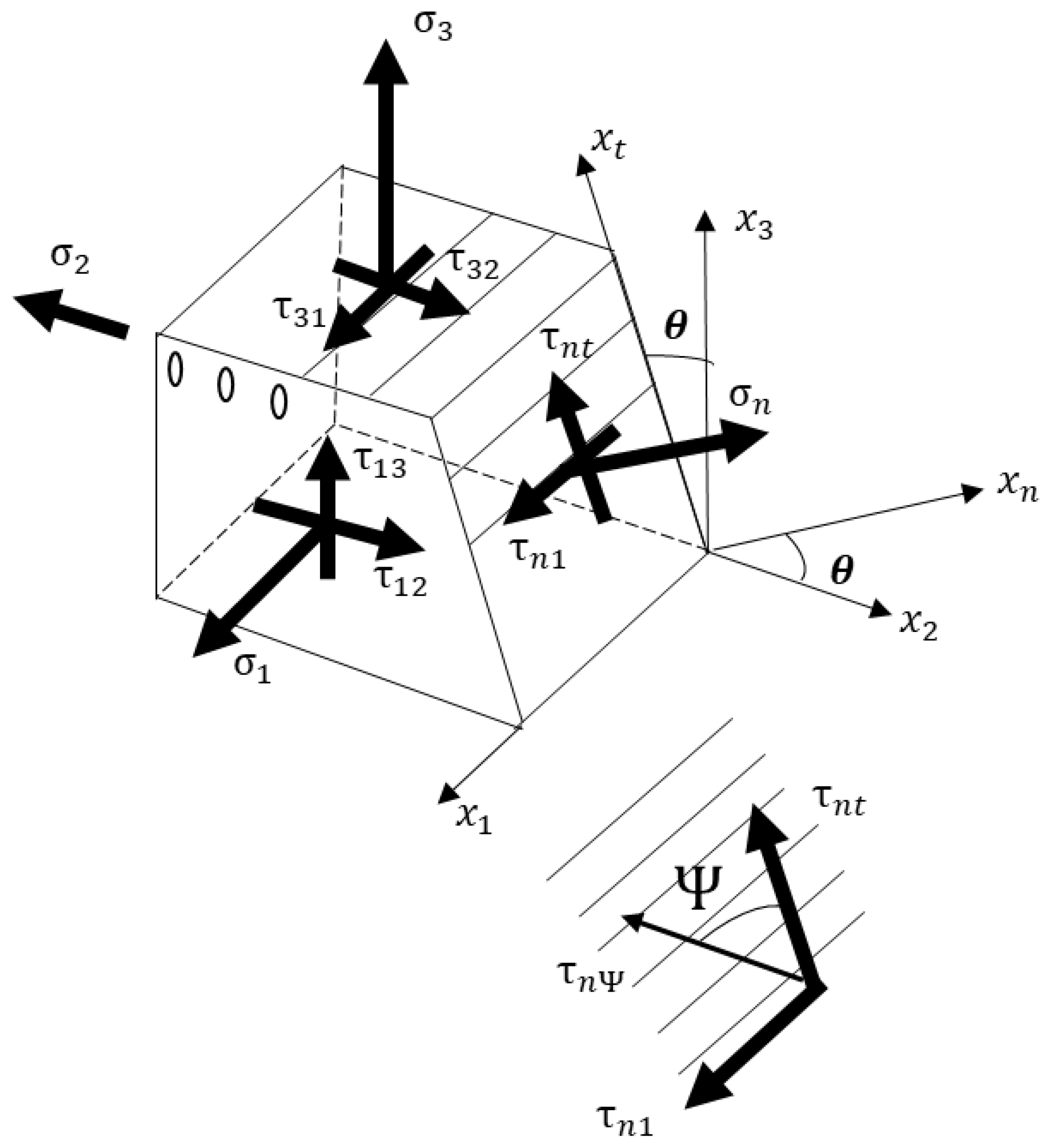
2.2.3. Puck Criterion

The Puck criterion is also an interactive failure criterion [23]. The relations representing this criterion can be written as:

• Tensile Fiber Failure

  $${\mathit{F}}_{\mathbf{1}}^{\mathit{T}\mathit{r}\mathit{a}\mathit{c}}={\left(\frac{{\mathbf{\sigma }}_{\mathbf{11}}}{{\mathit{X}}_{\mathit{t}}}\right)}^{\mathbf{2}}+{\left(\frac{{\mathbf{\tau }}_{\mathbf{12}}}{\mathit{S}}\right)}^{\mathbf{2}}=\mathbf{1}\hspace{1em}\left({\mathbf{\sigma }}_{\mathbf{11}}>\mathbf{0}\right)$$

  (36)
• Compressive Fiber Failure

  $${\mathit{F}}_{\mathbf{1}}^{\mathit{C}\mathit{o}\mathit{m}\mathit{p}\mathit{r}}={\left(\frac{{\mathbf{\sigma }}_{\mathbf{11}}}{{\mathit{X}}_{\mathit{t}}}\right)}^{\mathbf{2}}=\mathbf{1}\hspace{1em}\left({\mathbf{\sigma }}_{\mathbf{11}}<\mathbf{0}\right)$$

  (37)
• Tensile Matrix Failure

Damage initiation and evolution for tensile matrix cracking are defined using the following failure criteria:

$${\mathit{F}}_{\mathbf{2}}^{\mathit{T}\mathit{r}\mathit{a}\mathit{c}}={\left(\frac{{\mathbf{\sigma }}_{\mathbf{22}}}{{\mathit{Y}}_{\mathit{t}}}\right)}^{\mathbf{2}}+{\left(\frac{{\mathbf{\tau }}_{\mathbf{12}}}{{\mathit{S}}_{\mathbf{12}}}\right)}^{\mathbf{2}}+{\left(\frac{{\mathbf{\tau }}_{\mathbf{23}}}{{\mathit{S}}_{\mathbf{23}}}\right)}^{\mathbf{2}}\mathbf{=}\mathbf{1}\hspace{1em}\hspace{1em}\left({\mathbf{\sigma }}_{\mathbf{22}}>\mathbf{0}\right)$$

(38)

• Compressive Matrix Failure

For a general plane l-n-t with fracture angle ${\mathbf{\theta }}_{\mathit{f}}$, as shown (Figure 3), the stresses can be found according to the transformation from laminate coordinate systems 1-2-3 to x-y-z:

$$\{\begin{array}{c}{\mathbf{\sigma }}_{\mathit{n}\mathit{n}}={\mathbf{\sigma }}_{\mathit{y}}\mathit{c}\mathit{o}{\mathit{s}}^{\mathbf{2}}{\mathbf{\theta }}_{\mathit{f}}+{\mathbf{\sigma }}_{\mathit{z}}\mathit{s}\mathit{i}{\mathit{n}}^{\mathbf{2}}{\mathbf{\theta }}_{\mathit{f}}+\mathbf{2}{\mathbf{\tau }}_{\mathit{y}\mathit{z}}\mathit{c}\mathit{o}\mathit{s}{\mathbf{\theta }}_{\mathit{f}}\mathit{s}\mathit{i}\mathit{n}{\mathbf{\theta }}_{\mathit{f}}\\ {\mathbf{\tau }}_{\mathit{n}\mathit{l}}={\mathbf{\tau }}_{\mathit{y}\mathit{z}}\mathit{c}\mathit{o}\mathit{s}{\mathbf{\theta }}_{\mathit{f}}+{\mathbf{\tau }}_{\mathit{z}\mathit{x}}\mathit{c}\mathit{o}\mathit{s}{\mathbf{\theta }}_{\mathit{f}}\\ {\mathbf{\tau }}_{\mathit{n}\mathit{t}}=\left({\mathbf{\sigma }}_{\mathit{z}}-{\mathbf{\sigma }}_{\mathit{y}}\right)\mathit{c}\mathit{o}\mathit{s}{\mathbf{\theta }}_{\mathit{f}}\mathit{s}\mathit{i}\mathit{n}{\mathbf{\theta }}_{\mathit{f}}+{\mathbf{\tau }}_{\mathit{y}\mathit{z}}\left(\mathit{c}\mathit{o}{\mathit{s}}^{\mathbf{2}}{\mathbf{\theta }}_{\mathit{f}}-\mathit{s}\mathit{i}{\mathit{n}}^{\mathbf{2}}{\mathbf{\theta }}_{\mathit{f}}\right)\end{array}$$

(39)

Puck proposed a criterion for simulating transverse failure in a damage model taking into account the compressive load. The proposed failure criterion is similar to Hashin’s criteria with two main variations:

To calculate the failure occurrence, the tractions at the fracture plane ${\mathbf{\sigma }}_{\mathit{n}\mathit{n}}$, ${\mathbf{\tau }}_{\mathit{n}\mathit{l}}$, ${\mathbf{\tau }}_{\mathit{n}\mathit{t}}$ should not be associated with the nominal measured strengths from conventional mechanical tests, but with strengths corresponding to the fracture plane.

Normal compressive stress at the fracture did not cause the failure directly, while contributing to the increase of shear strength. The criterion is used to define the damage initiation.

$${\mathit{F}}_{\mathbf{2}}^{\mathit{C}\mathit{o}\mathit{m}\mathit{p}\mathit{r}}={\left(\frac{{\mathbf{\tau }}_{\mathit{n}\mathit{t}}}{{\mathit{S}}_{\mathbf{23}}{}^{\mathit{A}}-{\mathbf{\mu }}_{\mathit{n}\mathit{t}}{\mathbf{\sigma }}_{\mathit{n}\mathit{n}}}\right)}^{\mathbf{2}}+{\left(\frac{{\mathbf{\tau }}_{\mathit{n}\mathit{l}}}{{\mathit{S}}_{\mathbf{12}}-{\mathbf{\mu }}_{\mathit{n}\mathit{l}}{\mathbf{\sigma }}_{\mathit{n}\mathit{n}}}\right)}^{\mathbf{2}}=\mathbf{1}\hspace{1em}\left({\mathbf{\sigma }}_{\mathbf{22}}<\mathbf{0}\right)$$

(40)

where ${\mathit{S}}_{\mathbf{12}}$ is the longitudinal shear strength; ${\mathit{S}}_{\mathbf{23}}{}^{\mathit{A}}$ is the transverse shear strength in the potential fracture plane; ${\mathbf{\mu }}_{\mathit{n}\mathit{t}}$ and ${\mathbf{\mu }}_{\mathit{n}\mathit{l}}$ are friction coefficients in the transverse and longitudinal directions. These parameters are related to the fracture angle:

$$\mathbf{\phi }=\mathbf{2}{\mathbf{\theta }}_{\mathit{f}}-\mathbf{90}°; {\mathbf{\mu }}_{\mathit{n}\mathit{t}}=\mathit{t}\mathit{a}\mathit{n}\mathbf{\phi }$$

(41)

$${\mathit{S}}_{\mathbf{23}}{}^{\mathit{A}}=\frac{{\mathit{Y}}_{\mathit{c}}\left(\mathbf{1}-\mathit{s}\mathit{i}\mathit{n}\mathbf{\phi }\right)}{\mathbf{2}\mathit{c}\mathit{o}\mathit{s}\mathbf{\phi }} ; {\mathbf{\mu }}_{\mathit{n}\mathit{l}}={\mathbf{\mu }}_{\mathit{n}\mathit{t}}\frac{{\mathit{S}}_{\mathbf{12}}}{{\mathit{S}}_{\mathbf{23}}{}^{\mathit{A}}}$$

(42)

$$\begin{gathered} {\mathbf{\epsilon }}_{\mathit{n}\mathit{t}}={\mathbf{\gamma }}_{\mathbf{12}}\mathit{c}\mathit{o}\mathit{s}{\mathbf{\theta }}_{\mathit{f}}+{\mathbf{\gamma }}_{\mathbf{13}}\mathit{s}\mathit{i}\mathit{n}{\mathbf{\theta }}_{\mathit{f}}; \\ {\mathbf{\epsilon }}_{\mathit{n}\mathit{l}}=-{\mathbf{\epsilon }}_{\mathbf{22}}\mathit{c}\mathit{o}\mathit{s}{\mathbf{\theta }}_{\mathit{f}}\mathit{s}\mathit{i}\mathit{n}{\mathbf{\theta }}_{\mathit{f}}+{\mathbf{\epsilon }}_{\mathbf{33}}\mathit{c}\mathit{o}\mathit{s}{\mathbf{\theta }}_{\mathit{f}}\mathit{s}\mathit{i}\mathit{n}{\mathbf{\theta }}_{\mathit{f}}+{\mathbf{\gamma }}_{\mathbf{23}}\mathit{s}\mathit{i}\mathit{n}{\mathbf{\theta }}_{\mathit{f}}\left(\mathit{c}\mathit{o}{\mathit{s}}^{\mathbf{2}}{\mathbf{\theta }}_{\mathit{f}}-\mathbf{1}\right) \end{gathered}$$

(43)

where ${\mathit{Y}}_{\mathit{c}}$ is the standard transverse compressive strength.

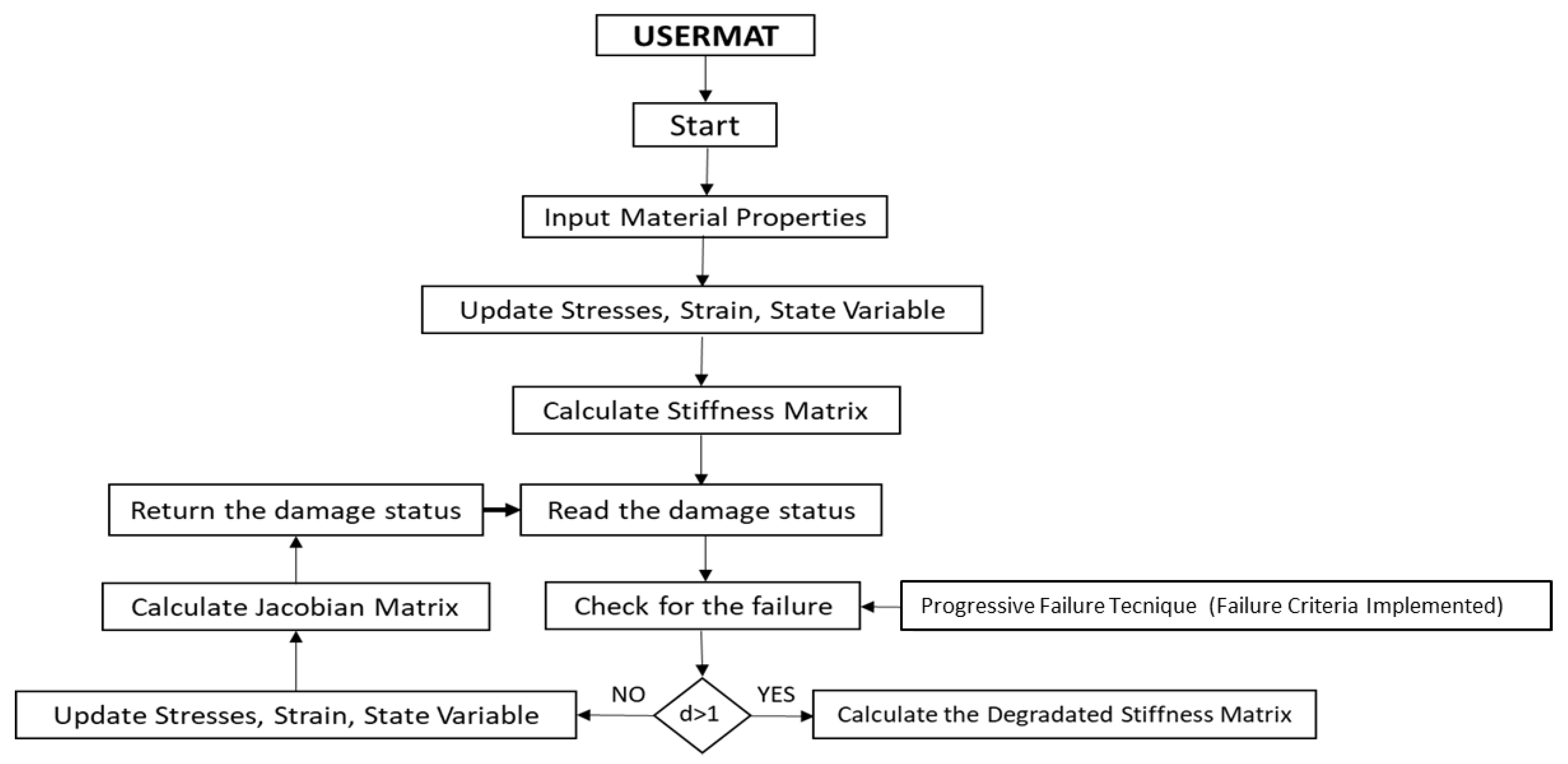
2.3. Finite Element Implementation: USERMAT

In the frame of simulations, the value of damage variables (Equation (27)) is evaluated and stored by the USERMAT, which is a user-programmable material (FORTRAN) sub-routine introduced in the ANSYS FEM [24]. This routine contributes to the description of the material in the frame of FEM analyses, including the evaluation of stress-strain relations. For every iteration, for each integration point the USERMAT subroutine evaluates the stresses and the state (damage) variables, according to specific user defined relations.

In the implemented USERMAT, three different criteria have been introduced: Hashin, maximum stress, and Puck’s criterion. It is possible to make a choice at the beginning of the analysis among the failure criteria and the degradation models (sudden or gradual).

The revised stress and strain variables are computed at integration points and a specific stress-strain relationship is forced by changing of the stiffness matrix. A schematic representation of the USERMAT operation is provided in the flow chart of Figure 4.

3. Numerical Applications

As already remarked, the numerical simulations have been performed on two literature test cases: an open hole tensile specimen (OHT) and a notched stiffened panel under shear loading conditions. To verify the effectiveness and accuracy of the intralaminar criteria and degradation models, the USERMAT is used to reproduce the mechanical response of these specimens. A preliminary description of the test cases with some considerations on the mesh convergence analysis, performed to reduce the computational time without compromises on accuracy of results, is also given in this section.

For the first application, it has been considered an element (Figure 5) with a single ply at 0° (in the same direction of fiber) characterized by AS4/PEEK material (

Table 1. Properties AS4/PEEK.

Property	Value
${\mathit{E}}_{\mathbf{1}}$ (longitudinal Young’s modulus)	127.6 GPa
${\mathit{E}}_{\mathbf{2}}$ (transverse Young’s modulus)	10.3 GPa
${\mathit{E}}_{\mathbf{3}}$ (transverse Young’s modulus)	10.3 GPa
${\mathbf{\nu }}_{\mathbf{12}}={\mathbf{\nu }}_{\mathbf{13}}={\mathbf{\nu }}_{\mathbf{23}}$ (Poisson’ s ratio)	0.32
${\mathit{G}}_{\mathbf{12}}$ (In-plane shear modulus)	6.0 GPa
${\mathit{G}}_{\mathbf{13}}$ (Out-of-plane shear modulus)	6.0 GPa
${\mathit{G}}_{\mathbf{23}}$ (Out-of-plane shear modulus)	3.0 GPa
${\mathit{X}}_{\mathit{t}}$ (longitudinal tensile strength)	2023 MPa
${\mathit{X}}_{\mathit{c}}$(longitudinal compressive strength)	1234 MPa
${\mathit{Y}}_{\mathit{t}}$ (transverse tensile strength)	92.7 MPa
${\mathit{Y}}_{\mathit{c}}$ (transverse compressive strength)	176 MPa
${\mathit{S}}_{\mathbf{12}}$ (In-plane shear strength)	82.6 MPa
${\mathit{S}}_{\mathbf{13}}$ (Out-of-plane shear strength)	82.6 MPa
${\mathit{S}}_{\mathbf{23}}$ (Out-of-plane shear strength)	82.6 MPa

).

In the ${\mathbf{\sigma }}_{\mathbf{11}}$-displacement curve (Figure 6) the maximum value of stress corresponds to ${\mathit{X}}_{\mathit{t}}$ value (longitudinal tensile strength of material).

The curves follow the pattern of sudden and gradual degradation. Immediately after the load falls, there is an increase in the curve caused by the damage variable not being equal to 1, and the elements have a residual stiffness that creates resistance and elastic return. This is an unreasonable situation, but this part of the curve is not relevant, it is important that first there is a gradual or sudden drop in the curve.

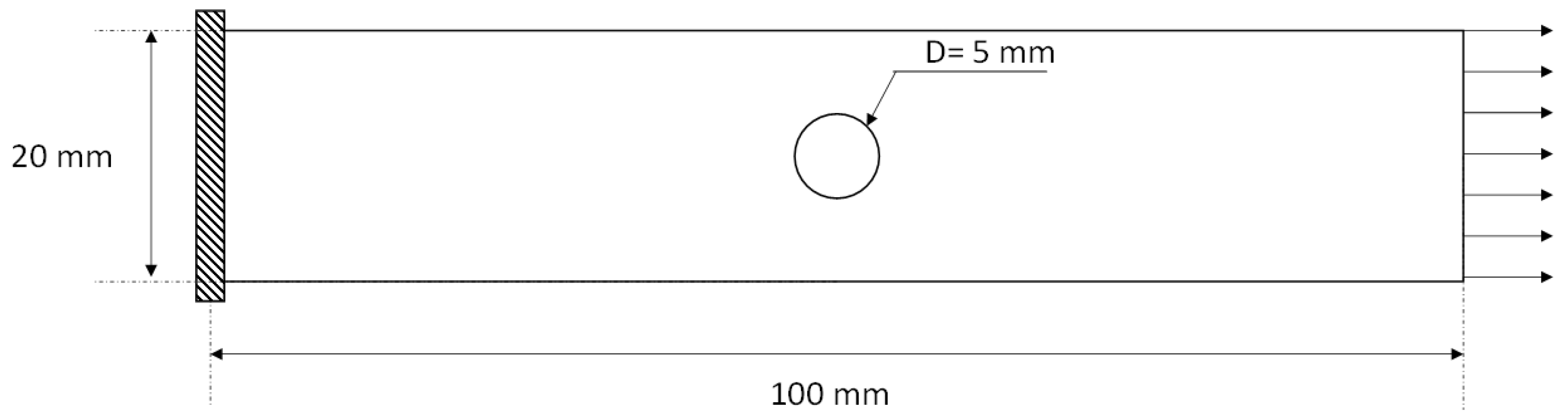
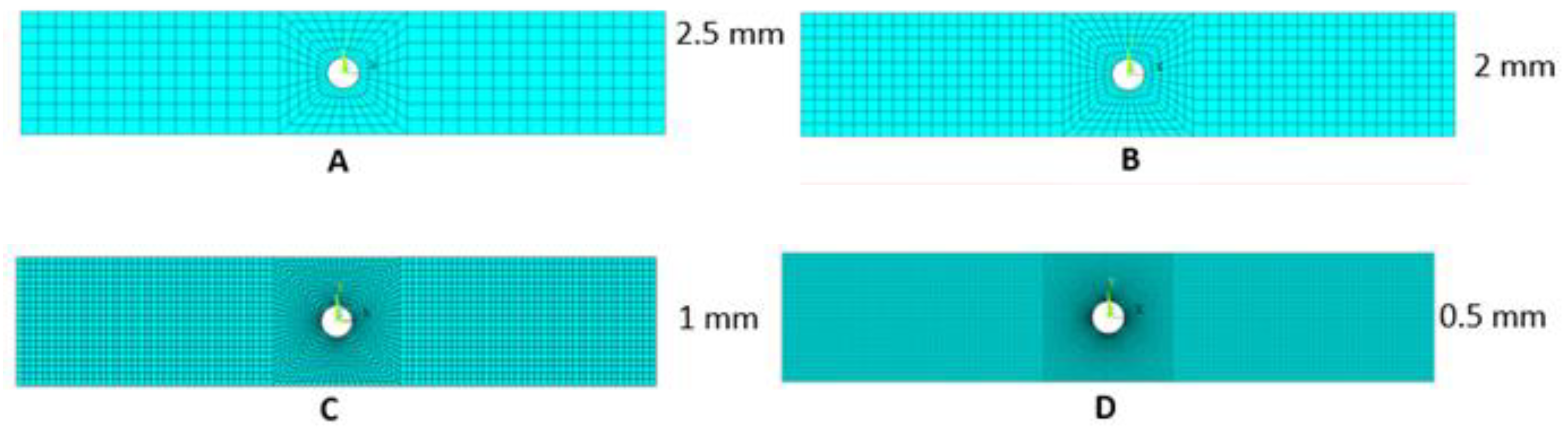
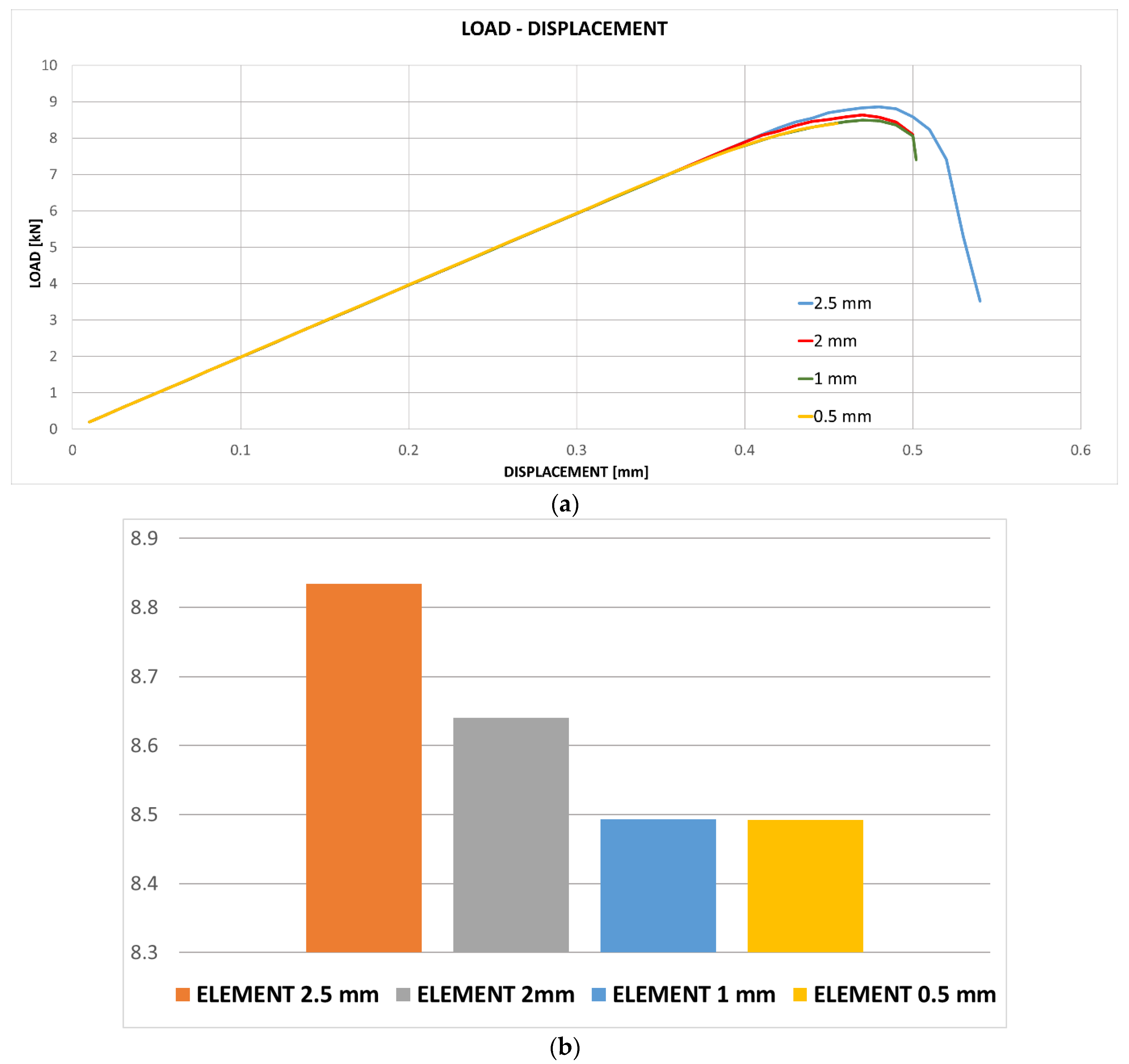
3.1. Open Hole Tensile (OHT)—Description of the FEM Model and Mesh Convergency

The geometry of the open hole tension specimen model is described in Figure 7 and the material properties of the lamina are listed in Table 1 [25].

The specimen is made with a composite laminate of 16 plies (material—AS4/PEEK) with a quasi-isotropic stacking sequence [0,45,90, −45]_2s. The thickness of single ply is 0.125 mm. The laminate has been modelled with SOLID186 3D layered elements.

A mesh convergency analysis has been performed by comparing four configurations, as showed in Figure 8 with different element sizes (2.5 mm—conf. A, 2 mm—conf. B, 1 mm—conf. C, 0.5 mm—conf. D). The ultimate load with a sudden degradation model and Hashin failure criteria has been considered as control parameter for convergence.

By performing this limited mesh sensitivity analysis, in Figure 9, where the load-displacement curves are introduced, it can be noted that the convergence of the mesh is reached for an element size of 1 mm. Indeed, a further decrease in the element size does not lead to an increase in accuracy (in terms of failure load). The choice of 1 mm element size is more suitable and reduces the computational cost.

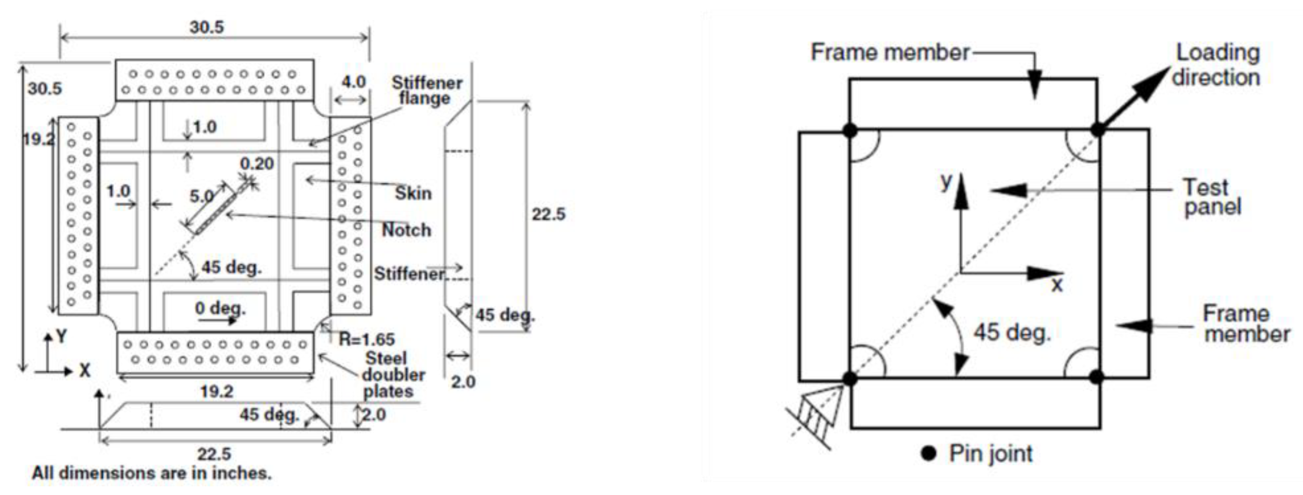
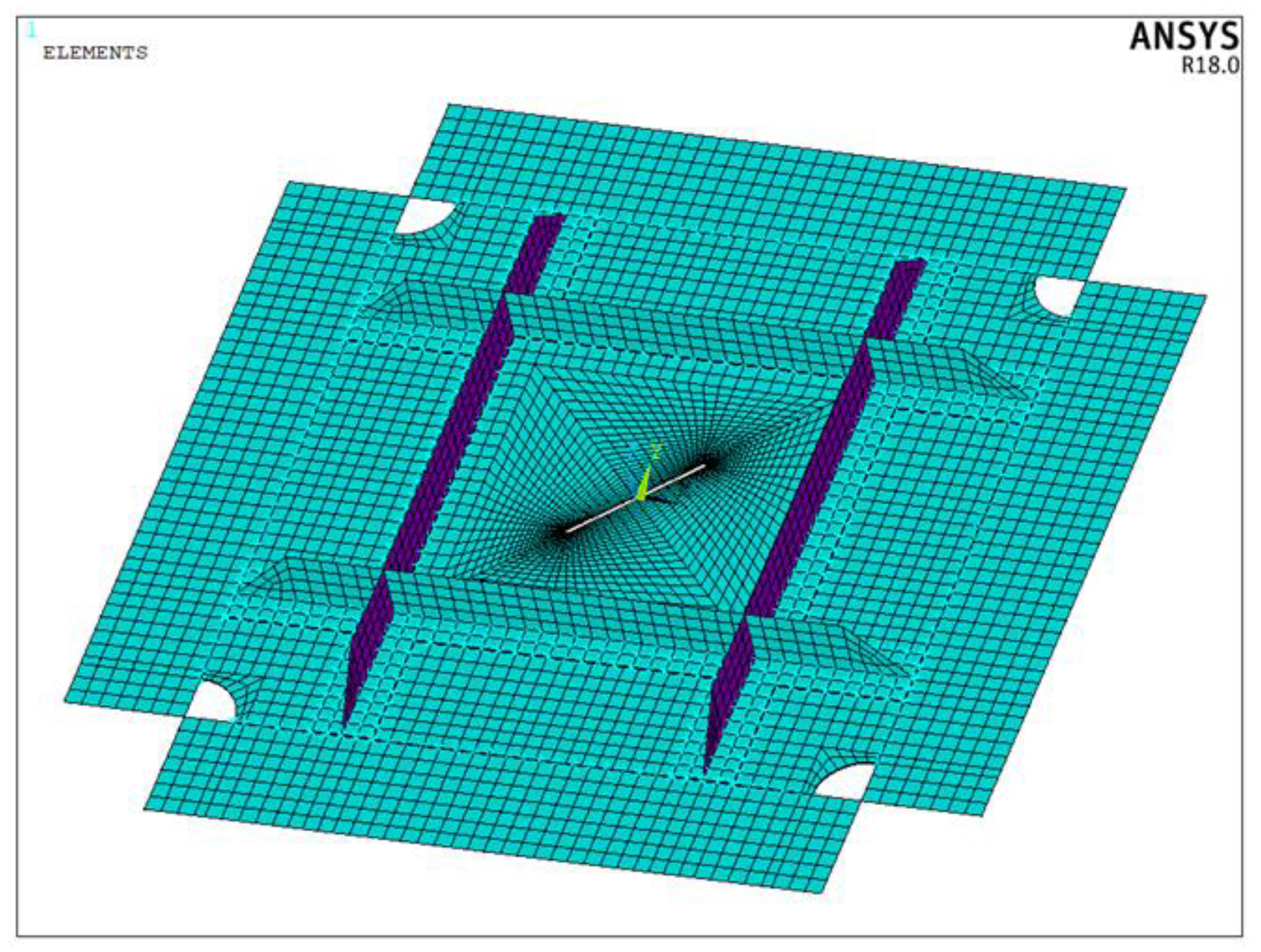
3.2. Notched Stiffened Panel under Shear Loading—Description of the FEM Model

A stiffened panel with a notch along its diagonal under shear loading condition has been taken as second test case to test the influence of failure criteria and Progressive Damage Models on the prediction of the mechanical behavior of composite laminates with evolving intralaminar damage. The geometry is shown in Figure 10 [26]. The material adopted for the manufacturing of skin and stiffeners is the AS4/3501-6 graphite-epoxy material system whose properties are shown in

Table 2. Property of AS4-3501/6.

Property	Value
${\mathit{E}}_{\mathbf{1}}$ (longitudinal Young’s modulus)	112.2 GPa
${\mathit{E}}_{\mathbf{2}}$ (transverse Young’s modulus)	11.0 GPa
${\mathit{E}}_{\mathbf{3}}$ (transverse Young’s modulus)	11.0 GPa
${\mathbf{\nu }}_{\mathbf{12}}={\mathbf{\nu }}_{\mathbf{13}}={\mathbf{\nu }}_{\mathbf{23}}$ (Poisson’ s ratio)	0.34
${\mathit{G}}_{\mathbf{12}}$ (In-plane shear modulus)	5.5 GPa
${\mathit{G}}_{\mathbf{13}}$ (Out-of-plane shear modulus)	5.5 GPa
${\mathit{G}}_{\mathbf{23}}$ (Out-of-plane shear modulus)	2.7 GPa
${\mathit{X}}_{\mathit{t}}$ (longitudinal tensile strength)	1422 MPa
${\mathit{X}}_{\mathit{c}}$(longitudinal compressive strength)	1034 MPa
${\mathit{Y}}_{\mathit{t}}$ (transverse tensile strength)	34.5 MPa
${\mathit{Y}}_{\mathit{c}}$ (transverse compressive strength)	213.7 MPa
${\mathit{S}}_{\mathbf{12}}$ (In-plane shear strength)	120.6 MPa
${\mathit{S}}_{\mathbf{13}}$ (Out-of-plane shear strength)	33.1 MPa
${\mathit{S}}_{\mathbf{23}}$ (Out-of-plane shear strength)	33.1 MPa

. The stacking sequence of the skin is ${\left[45/-45/0/90\right]}_s$, while the stacking sequence of the stiffener flanges and blades are ${\left[\left(45/-45/0/90\right)2\right]}_s$ and ${\left[\left(45/-45/0/90\right)3\right]}_s$, respectively.

The thickness of single ply is 0.182 mm. The panel has been modelled with SOLID186 3D layered elements. A limited mesh sensitivity analysis has been carried out similar to the one performed for the open tensile specimen. In the frame of this analysis, which is not reported here for the sake of brevity, an optimal element size of 1 mm has been found and adopted for the rest of the analyses (see Figure 11).

4. Results and Discussion

In this section, the numerical results obtained for the two analyzed test cases are illustrated and examined. The scope is to assess the influence of Progressive Degradation Models and failure criteria on accuracy in predicting the intralaminar damage evolution in composite laminates. The results obtained for the two test cases are presented in the next subsections.

4.1. Numerical Results—Open Hole Tension Specimen

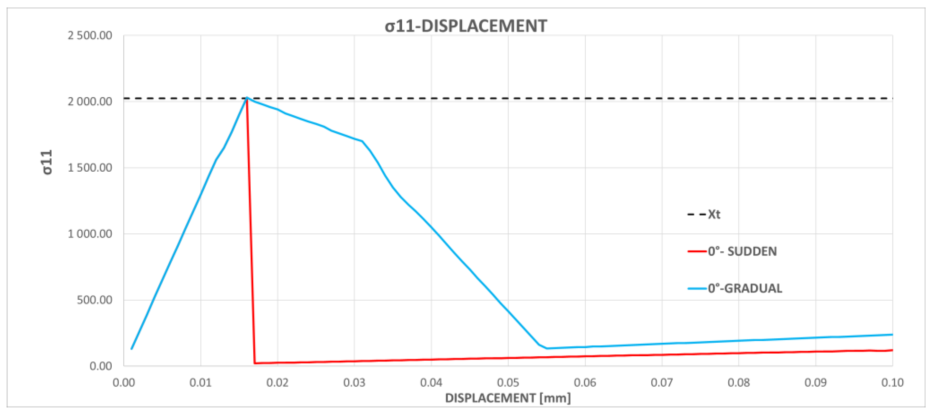
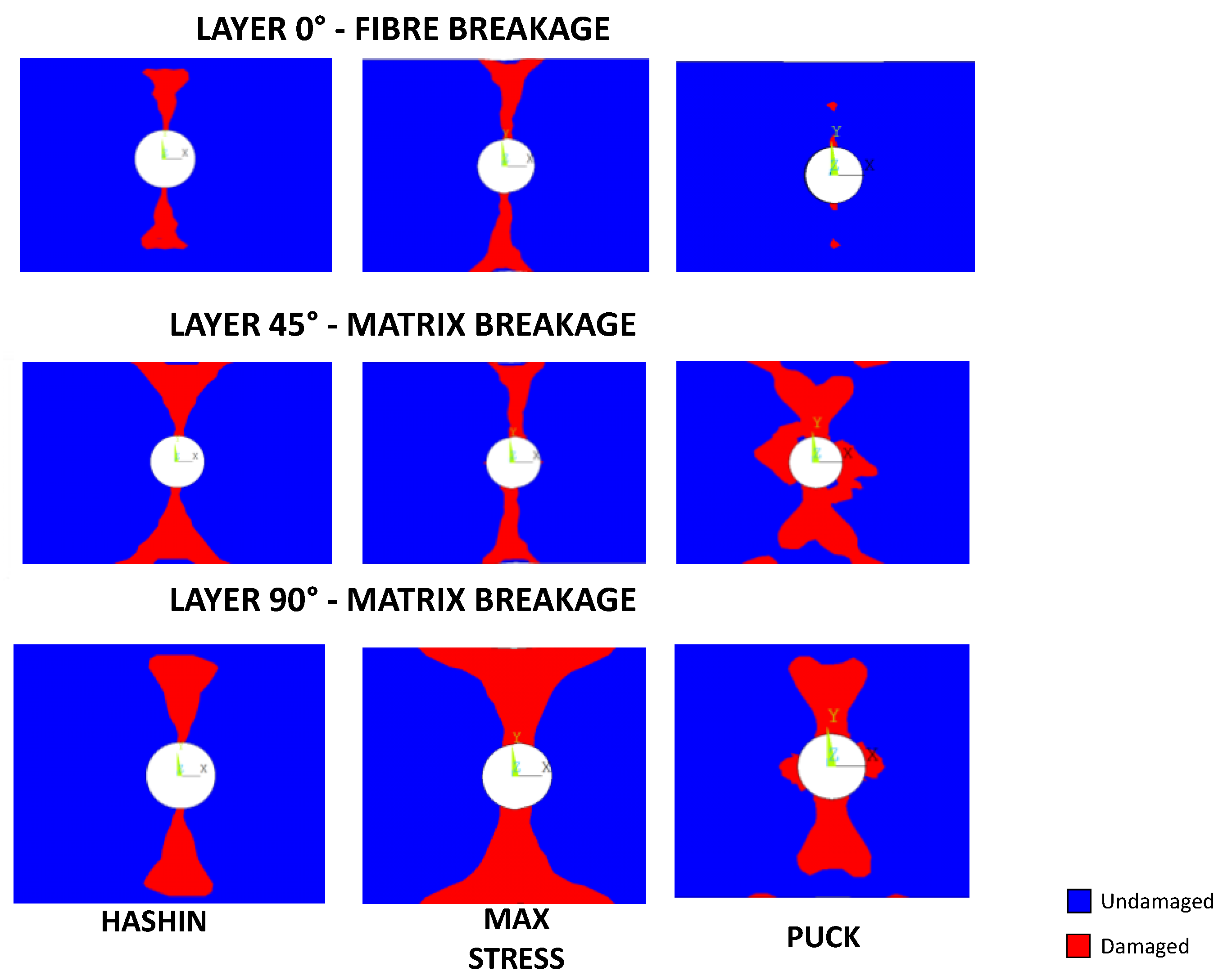
4.1.1. Instantaneous (Sudden) Progressive Degradation Model

First, a non-linear static finite element simulation has been performed on the Open Hole Tension test case by adopting an Instantaneous Progressive Degradation Model. In Figure 11, the load displacement curves obtained by adopting the three analyzed different criteria are presented. In reality, the numerical results obtained, in terms of maximum load to failure, are not in good agreement with each other and with the experimental failure load of 15 kN found by Maa et al. [27]. As shown in

Table 3. Comparison of maximum load: sudden degradation.

Sudden Degradation Law
Evaluated Cases	Value of Maximum Load
Experimental	15.1 kN
Fem Maa et al.	12 kN
Maximum Stress Criterion	12.176 kN
Puck’s Criterion	11.16 kN
Hashin Criterion	8.49 kN

, all the failure criteria underestimate the experimental failure load. Indeed, the maximum stress criterion provides numerical results very close to the ones obtained with the numerical model introduced in [21].

As expected, the maximum stress criterion provides a higher failure load if compared with Hashin and Puck criterion. This can be simply explained by comparing Equations (32) and (36) to Equation (28) due to the introduction of the contribution of shear stress for fiber tensile damage. In Reddy and Reddy [28], it is shown that that the maximum stress criterion overestimates failure loads for composites under axial tension.

When adopting Instantaneous Progressive Degradation Models, a sudden drop in the load–displacement curve can be appreciated, which reflects the sudden degradation of material properties in terms of axial stiffness, as shown in Figure 12. It can be observed that Puck’s criterion considers all failure modes and their interaction, while maximum stress is a mode separate criterion.

As can be appreciated in Figure 11, the Hashin and maximum stress criteria have a similar trend in terms of damaged area shape at failure both for fiber and matrix damage. For matrix damage at 45° oriented plies, the maximum stress criterion underestimates the damaged area as an envelope of completely failed elements (which is plotted in red in Figure 13, being the blue region representative of undamaged elements) when compared to the Hashin failure criteria. For all the other layers and failure modes, the maximum stress criterion overestimates the damaged area when compared to the Hashin failure criteria. The trend obtained with Puck criterion seems not to be completely physically based, especially for matrix damage in plies oriented at 45°.

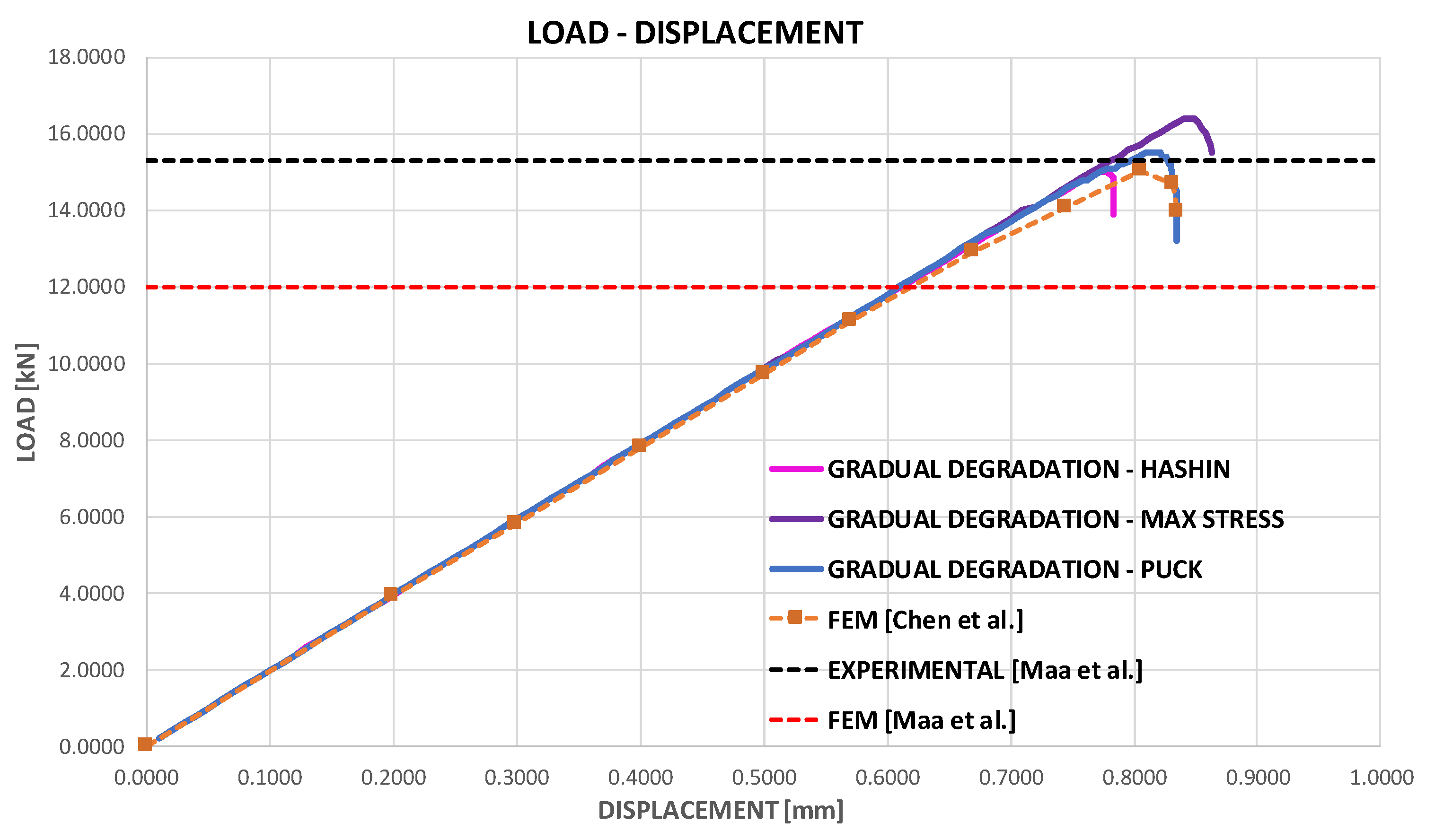
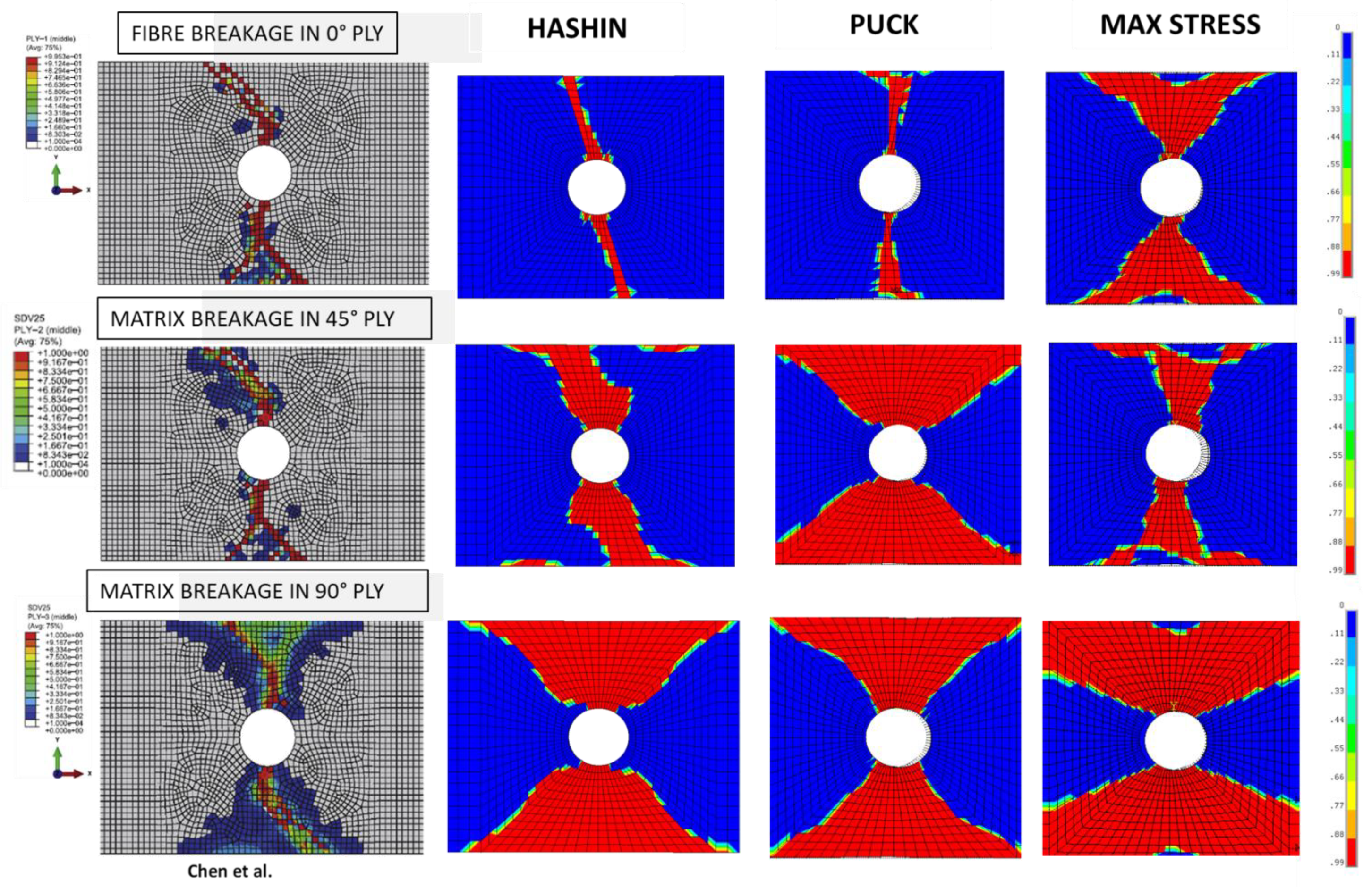
4.1.2. Gradual Degradation Model—OHT

A non-linear static finite element simulation was then performed on the Open Hole Tension test case by adopting a Gradual Progressive Degradation Model. In Figure 14, the load displacement curves obtained by adopting the three different analyzed criteria are presented. The numerical results obtained, in terms of maximum load to failure, are in excellent agreement with each other and with the experimental failure load of 15 kN found by Maa et al. [27]. As shown in

Table 4. Comparison of maximum load: gradual degradation.

Gradual Degradation Law
Evaluated Cases	Value of Maximum Load
Experimental	15.1 kN
Fem Maa et al.	12 kN
Fem Chen et al.	15.038 kN
Maximum Stress Criterion	16.4 kN
Puck’s Criterion	15.5 kN
Hashin Criterion	15 kN

, all the failure criteria are very close to the experimental failure load. Indeed, the Hashin stress criterion provide the best numerical results which are closest to the experimental data. On the contrary, the maximum stress overestimates the maximum load since this criterion belongs to the family of separate modes criteria. Hence, the failure in one direction is only related to the stress state in that particular direction, which can result in an underestimation of the failure and, consequently, in an overestimation of the failure load. However, this criterion has been considered suitable to the application presented in this work due to the specific boundary conditions that produce a quasi-one-dimensional stress state.

In Figure 15, the numerical results obtained with the Gradual Progressive Damage Model, in terms of damaged area at failure for the different failure modes for the laminae of the quasi-isotropic laminate, are compared with numerical results from Chen et al. [16]. The numerical results obtained applying the maximum stress, Hashin, and Puck criteria are compared.

All the criteria provide very similar numerical results which are in agreement with literature numerical results of [16].

In particular, for laminae oriented at 0° (with fibers oriented along the load direction), as expected, the predictions, with all the investigated failure criteria, show that the damaged zone is smaller than the one of the other plies.

Hence, when adopting Gradual Progressive Damage Models, all the investigated failure criteria are suitable for calculating the global mechanical response of composite laminates undergoing intralaminar damage evolution under static loading conditions.

However, since the Hashin failure criterion is capable of guaranteeing the best results even when Instantaneous Progressive Degradation Models are adopted, only this criterion will be used for the next test case.

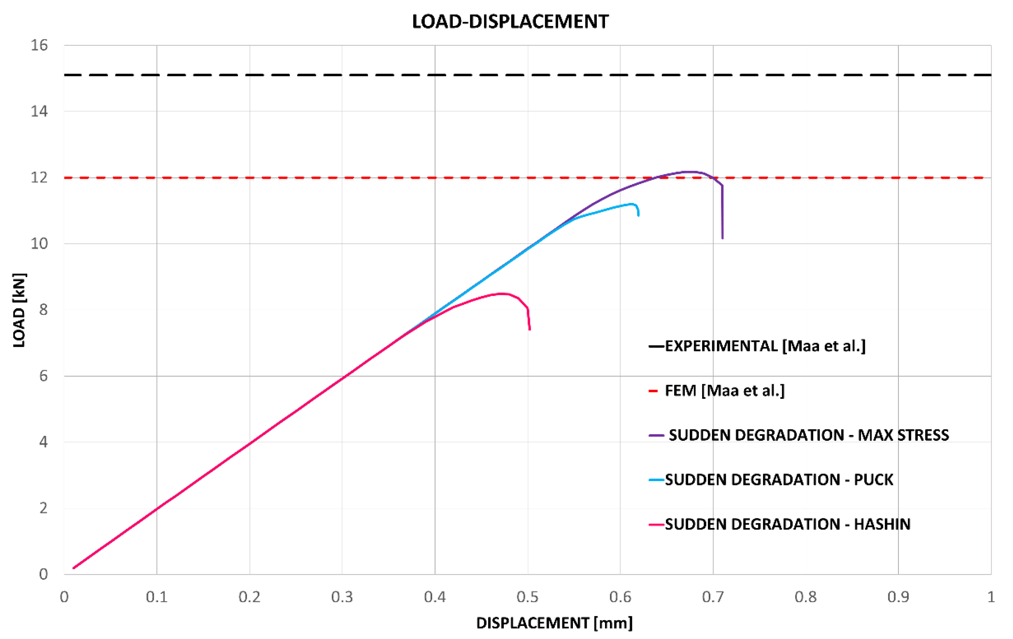
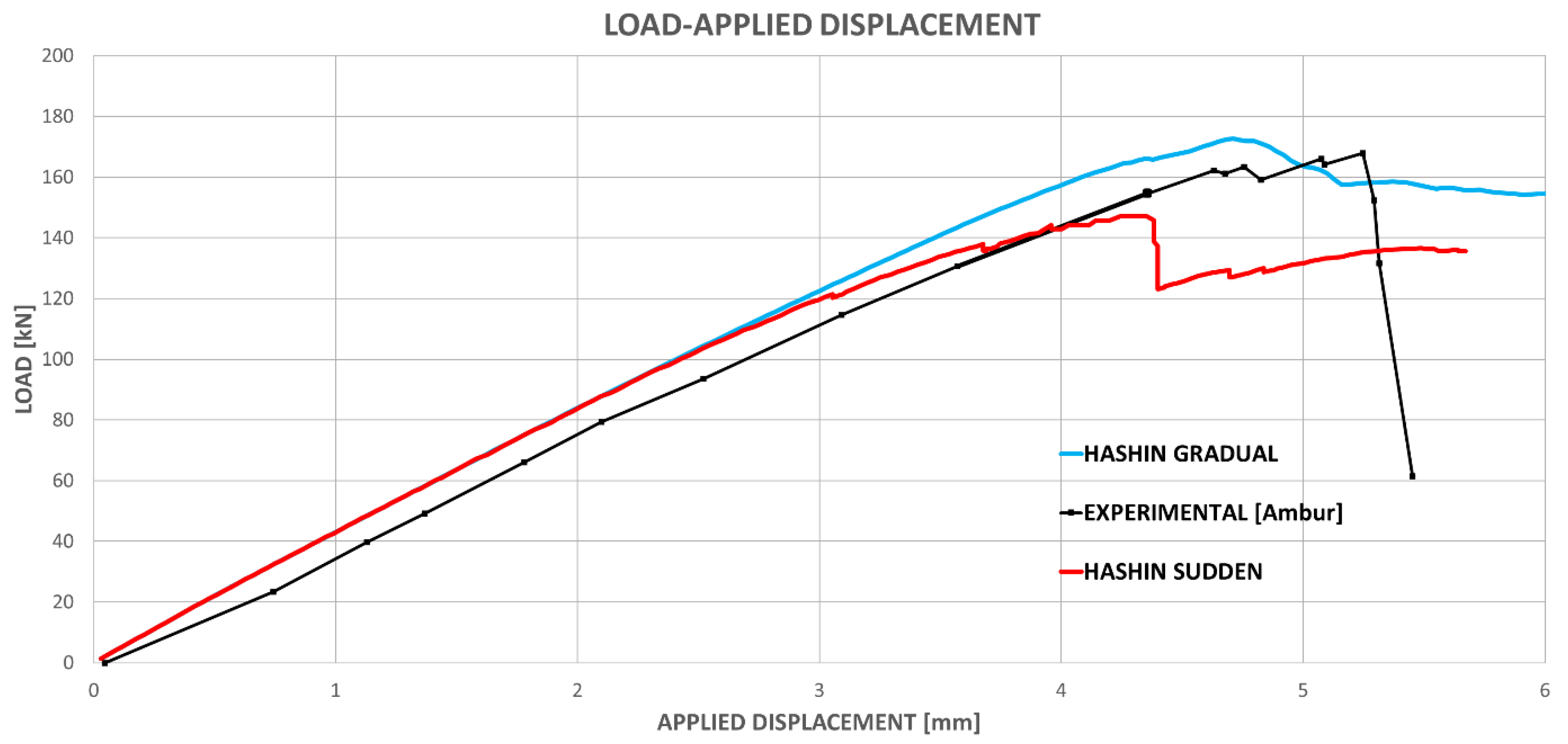
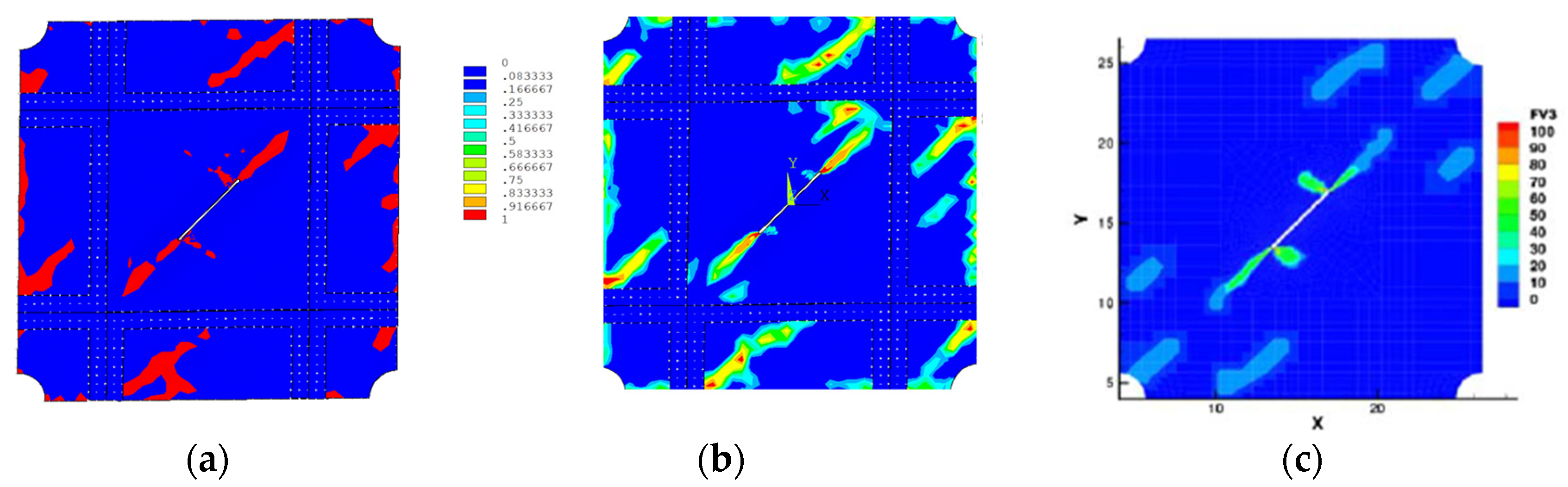
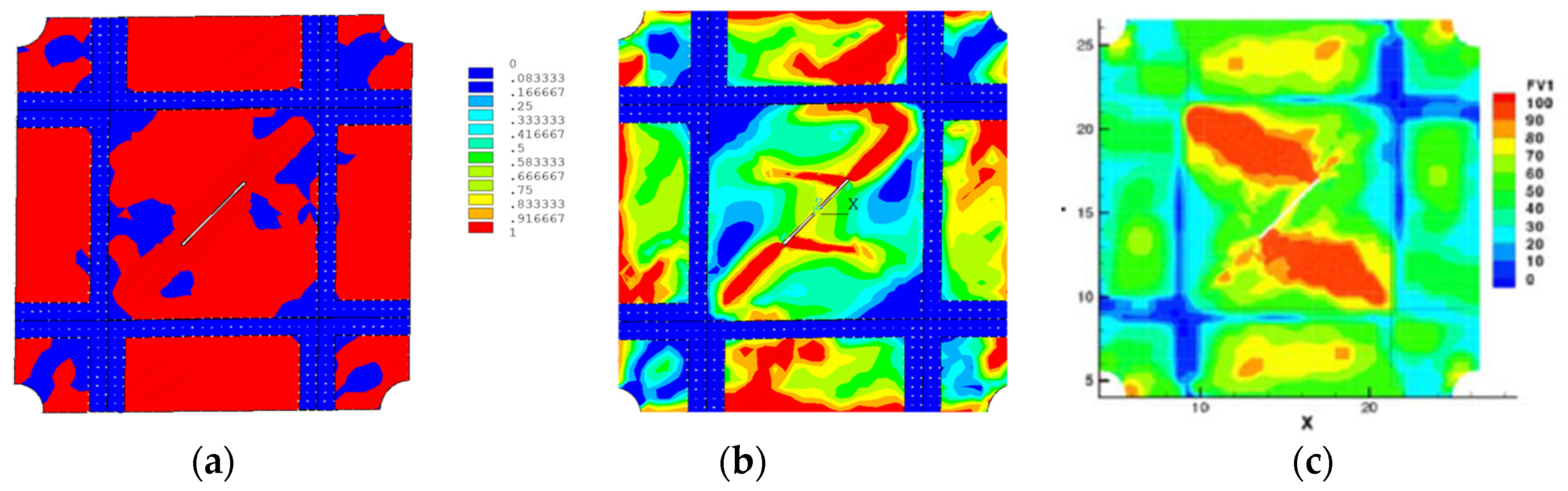
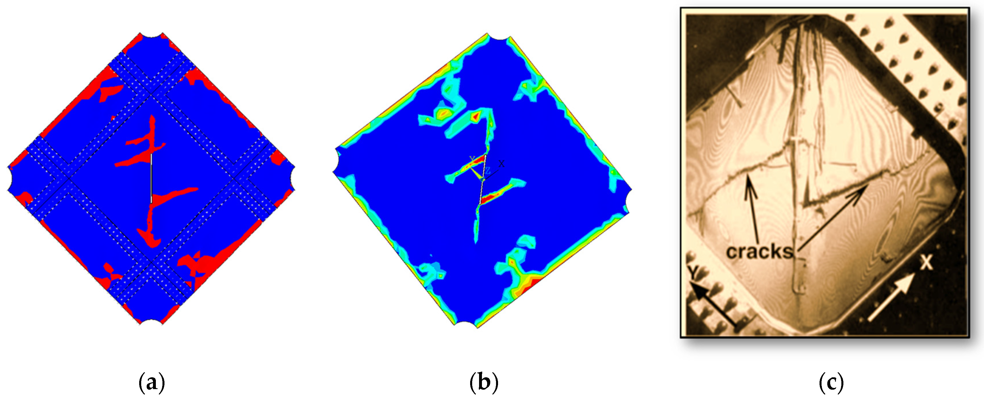
4.2. Notched Stiffened Panel under Shear Loading

As a second test case, a notched stiffened panel under shear loading has been analyzed. The mechanical behavior, including intralaminar damage onset and evolution, has been simulated by adopting the Hashin failure criteria to predict the damage onset. The evolution of the intralaminar damage, in terms of fiber and matrix failures, has then been simulated by adopting an Instantaneous Progressive Damage Model and a Gradual Progressive Damage Model. The numerical results obtained with these two Progressive Damage Models have been compared with literature experimental data to assess their effectiveness in predicting the shear mechanical behavior of the investigated stiffened panel.

In the Figure 16, the load displacement curves obtained with the Instantaneous (Sudden) Progressive Degradation Model and the Gradual Progressive Degradation Model are compared with the literature experimental data from [26]. As can be appreciated in the figure, the Sudden Model is not able to mimic the trend of the experimental curve. In particular, the predicted maximum load (145 kN) is substantially lower when compared to the experimental one (170 kN). On the other hand, the trend obtained with the Gradual Model is in excellent agreement with the experimental one, with a predicted maximum load (173 kN), which is very close to the experimental one. Both the curves are characterized by a persistent constant trend after failure that is related to the presence of a residual strength, due to residual low material properties introduced after the damage events according to both the formulations. These low residual material properties have been introduced for convergence purposes, but actually they have no physical meaning.

In Figure 17 and Figure 18, the fiber and matrix damage distributions in the panel (at failure), found with sudden and gradual models are compared with literature numerical results from [26]. For the sudden propagation, the damaged area with completely failed elements is colored in red, while for the gradual propagation, a contour plot of the damage variable is presented. As already seen for the open hole tension specimen, the damage area distributions obtained for the notched panel with the sudden and gradual propagation model are almost the same and in agreement with the numerical literature results and the macroscopic cracks observed during the experiment. Obviously, according to Figure 16, the damage status at failure of Figure 17 and Figure 18 occurs at different load levels in simulations with sudden and gradual progression models.

If all the damaged elements (with fiber and matrix failure) are represented in a single view, a useful overview of the panel damage status can be obtained. In Figure 19, an example of this damage representation is given. Actually, in Figure 19, the damage status at failure obtained with Sudden and Gradual Progressive Degradation Models is compared with the damage status of the failed notched panel taken from [26]. As can be appreciated, the numerical prediction of the crack direction is in excellent agreement with the experimental observed failure path arising from the notch edge and propagating along the direction of the applied shear load.

In Figure 19 it is also possible to notice that the damage at boundaries, when the shear load is applied, is very well predicted by both the numerical degradation models.

5. Conclusions

In this paper, a study on the influence of numerical models on the simulation of the mechanical behavior of composite laminates with intralaminar damage is introduced. In particular, the effects of failure criteria and Sudden and Gradual Progressive Degradation Models on the accuracy of numerical predictions, in terms of failure load and damage distributions, are investigated.

Two numerical test cases, an open hole tension specimen and a notched stiffened panel under shear loading, have been modeled and numerically tested by adopting a USERMAT subroutine implemented in FE code ANSYS. The numerical results obtained have been compared with literature experimental data.

The open hole specimen has been used to compare the numerical results obtained with three different failure criteria (maximum stress, Hashin, and Puck criteria). The Hashin failure criteria has been found to provide the more reliable result with both sudden and gradual progressive damage models.

However, for the open hole tension specimen, the Sudden Progressive Degradation Model has been proven to underestimate the failure load. This trend has been confirmed by the simulations performed for the more complex second test case. On the other hand, the Gradual Progressive Degradation Model has been found able to correctly mimic the experimental trends, in terms of load-displacement curve for the analyzed test cases.

Finally, from the simulations performed on both the test cases, the Hashin failure criteria has been found able to correctly determine the damage distributions in terms of fiber and matrix failure and to correctly follow the experimental damage propagation path.

At this stage, the focus was on finding differences between the failure criteria and the two degradation models in order to obtain more readable results. For the sake of brevity, future work can be carried out following the study comparing different degradation laws.

References

1. Sellitto, A.; Riccio, A.; Russo, A.; Zarrelli, M.; Toscano, C.; Lopresto, V. Compressive behaviour of a damaged omega stiffened panel: Damage detection and numerical analysis. Compos. Struct. 2019, 209, 300–316. [Google Scholar] [CrossRef]
2. Russo, A.; Sellitto, A.; Saputo, S.; Acanfora, V.; Riccio, A. Cross-influence between intra-laminar damages and fibre bridging at the skin-stringer interface in stiffened composite panels under compression. Materials 2019, 12, 1856. [Google Scholar] [CrossRef] [Green Version]
3. Sleight, D.W.; Knight, N.F., Jr.; Wang, J.T. Evaluation of a progressive failure analysis methodology for laminated composite structures. In 38th Structures, Structural Dynamics, and Materials Conference. Kissimmee, FL, USA, 7–10 April 1997; American Institute of Aeronautics and Astronautics: Reston, VA, USA, 1997. [Google Scholar] [CrossRef] [Green Version]
4. Lapczyk, I.; Hurtado, J.A. Progressive damage modeling in fiber-reinforced materials. Compos. Part A Appl. Sci. 2007, 38, 2333–2341. [Google Scholar] [CrossRef]
5. Sleight, D.W. Progressive Failure Analysis Methodology for Laminated Composite Structures; Technical Report for NASA; NASA: Hampton, VA, USA, 1 March 1999.
6. Hashin, Z. Failure criteria for unidirectional fiber composites. J. Appl. Mech. 1980, 47, 329–334. [Google Scholar] [CrossRef]
7. Chang, F.K.; Chang, K.Y. A progressive damage model for laminated composites containing stress concentrations. J. Compos. Mater. 1988, 21, 834–855. [Google Scholar] [CrossRef]
8. Hou, J.P.; Petrinic, N.; Ruiz, C. A delamination criterion for laminated composites under low-velocity impact. Compos. Sci. Technol. 2001, 61, 2069–2074. [Google Scholar] [CrossRef]
9. Puck, A.; Schürmann, H. Failure analysis of FRP laminates by means of physically based phenomenological models. Compos. Sci. Technol. 2002, 62, 1633–1662. [Google Scholar] [CrossRef]
10. De Luca, A.; Caputo, F. A review on analytical failure criteria for composite materials. AIMS Mater. Sci. 2017, 4, 1165–1185. [Google Scholar] [CrossRef]
11. Almeida, J.H.S., Jr.; Bittrich, L.; Spickenheuer, A. Improving the open-hole tension characteristics with variable-axial composite laminates: Optimization, progressive damage modeling and experimental observations. Compos. Sci. Technol. 2020, 185, 107889. [Google Scholar] [CrossRef]
12. Almeida, J.H.S., Jr.; Ribeiro, M.L.; Tita, V.; Campos Amico, S.C. Damage and failure in carbon/epoxy filament wound composite tubes under external pressure: Experimental and numerical approaches. Mater. Des. 2016, 96, 431–438. [Google Scholar] [CrossRef]
13. Almeida, J.H.S., Jr.; Ribeiro, M.L.; Tita, V.; Campos Amico, S.C. Damage modeling for carbon fiber/epoxy filament wound composite tubes under radial compression. Compos. Struct. 2017, 160, 204–210. [Google Scholar] [CrossRef]
14. Almeida, J.H.S., Jr.; Maikson, L.P.; Tonatto; Ribeiro, M.L.; Tita, V.; Amico, S.C. Buckling and post-buckling of filament wound composite tubes under axial compression: Linear, nonlinear, damage and experimental analyses. Compos. Part B Eng. 2018, 149, 227–239. [Google Scholar] [CrossRef]
15. Almeida, J.H.S., Jr.; Ribeiro, M.L.; Tita, V.; Amico, S.C. Stacking sequence optimization in composite tubes under internal pressure based on genetic algorithm accounting for progressive damage. Compos. Struct. 2017, 178, 20–26. [Google Scholar] [CrossRef]
16. Chen, J.-F.; Morozov, E.V.; Shankar, K. Simulating progressive failure of composite laminates including in-ply and delamination damage effects. Compos. Part A Appl. Sci. 2014, 61, 185–200. [Google Scholar] [CrossRef]
17. Ambur, D.R.; Jaunky, N.; Hilburger, M.W. Progressive failure studies of stiffened panels subjected to shear loading. Compos. Struct. 2004, 65, 129–142. [Google Scholar] [CrossRef] [Green Version]
18. Riccio, A.; Di Costanzo, C.; Di Gennaro, P.; Sellitto, A.; Raimondo, A. Intra-laminar progressive failure analysis of composite laminates with a large notch damage. Eng. Fail. Anal. 2016, 73, 97–112. [Google Scholar] [CrossRef]
19. Camanho, P.P.; Dávila, C.G. Mixed Mode Decohesion Finite Elements for the Simulation of Delamination in Composite Materials; Technical Report for NASA; NASA: Hampton, VA, USA, 1 June 2002.
20. Chang, K.-Y.; Liu, S.; Chang, F.-K. Damage Tolerance of Laminated Composites Containing an Open Hole and Subjected to Tensile Loadings. J. Compos. Mater. 1991, 25, 274–301. [Google Scholar] [CrossRef]
21. Rohwer, K. Models for Intralaminar damage and failure of fiber composites—A review. Facta Univ. Ser. Mech. Eng. 2016, 14, 1–19. [Google Scholar] [CrossRef]
22. Bažant, Z.P.; Oh, B.H. Crack-band theory for fracture of concrete. Mat. Constr. 1983, 16, 155–177. [Google Scholar] [CrossRef] [Green Version]
23. Puck, A.; Deuschle, H.M. Progress in the Puck failure theory for fibre reinforced composites: Analytical solutions for 3D-stress. J. Compos. Mater. 2013, 47, 827–846. [Google Scholar] [CrossRef]
24. Lin, G. ANSYS USER Material Subroutine USERMAT; ANSYS, Inc.: Canonsburg, PA, USA, November 1999. [Google Scholar]
25. Chen, D.L.; Weiss, B.; Stickler, R. A new geometric factor formula for a center cracked plate tensile specimen of finite width. Int. J. Fract. 1992, 55, R3–R8. [Google Scholar] [CrossRef]
26. Ambur, D.R.; Jaunky, N.; Davila, C.G.; Hilburger, M.W. Progressive Failure Studies of Composite Panels with and without Cutouts; Technical Report for NASA; NASA: Hampton, VA, USA, 1 September 2001.
27. Maa, R.-H.; Cheng, J.-H. A CDM-based failure model for predicting strength of notched composite laminates. Compos. Part B Eng. 2002, 33, 479–489. [Google Scholar] [CrossRef]
28. Pandey, A.; Reddy, J.A. Post First-Ply Failure Analysis of Composite Laminates. In 28th Structures, Structural Dynamics and Materials Conference, Monterey, CA, USA, 6–8 April 1987; American Institute of Aeronautics and Astronautics: Reston, VA, USA, 1987. [Google Scholar] [CrossRef]
Figure 1. Sudden degradation.
Jcs 05 00310 g001
Figure 2. Gradual degradation.
Jcs 05 00310 g002
Figure 3. Representation of Puck’s coordinate system.
Jcs 05 00310 g003
Figure 4. Flow chart of USERMAT.
Jcs 05 00310 g004
Figure 5. Single Element at 0°.
Jcs 05 00310 g005
Figure 6. σ 11 -displacement curve.
Jcs 05 00310 g006
Figure 7. Geometrical model Open Hole Tensile.
Jcs 05 00310 g007
Figure 8. Configuration of four different mesh sizes: (A)—2.5 mm, (B)—2 mm, (C)—1 mm, (D)—0.5 mm.
Jcs 05 00310 g008
Figure 9. Mesh sensitivity:(a) Load displacement curves; (b) Failure load values versus Element size.
Jcs 05 00310 g009
Figure 10. Geometrical model of Stiffened Panel.
Jcs 05 00310 g010
Figure 11. FEM model: stiffened panel.
Jcs 05 00310 g011
Figure 12. Load displacement curves for different criteria in Sudden Degradation Model.
Jcs 05 00310 g012
Figure 13. Fiber and matrix failure in each lamina for OHT (sudden degradation).
Jcs 05 00310 g013
Figure 14. Load displacement curves for different criteria in Gradual Degradation Model.
Jcs 05 00310 g014
Figure 15. Fiber and matrix failure in each lamina for OHT (Gradual degradation).
Jcs 05 00310 g015
Figure 16. Sudden and Gradual Degradation Models with Hashin failure criteria: comparison with experimental data [26].
Jcs 05 00310 g016
Figure 17. Fiber failure: (a) Sudden Degradation Model; (b) Gradual Degradation Model; (c) Literature numerical results [26].
Jcs 05 00310 g017
Figure 18. Matrix failure: (a) Sudden Degradation Model; (b) Gradual Degradation Model; (c) Literature numerical results [26].
Jcs 05 00310 g018
Figure 19. Failure Envelope: (a) Sudden Degradation Model, (b) Gradual Degradation Model, and (c) Literature experimental data [26].
Jcs 05 00310 g019