Evaluation of In Vivo Spike Detection Algorithms for Implantable MTA Brain—Silicon Interfaces

Abstract

This work presents a comparison between different neural spike algorithms to find the optimum for in vivo implanted EOSFET (electrolyte–oxide-semiconductor field effect transistor) sensors. EOSFET arrays are planar sensors capable of sensing the electrical activity of nearby neuron populations in both in vitro cultures and in vivo experiments. They are characterized by a high cell-like resolution and low invasiveness compared to probes with passive electrodes, but exhibit a higher noise power that requires ad hoc spike detection algorithms to detect relevant biological activity. Algorithms for implanted devices require good detection accuracy performance and low power consumption due to the limited power budget of implanted devices. A figure of merit (FoM) based on accuracy and resource consumption is presented and used to compare different algorithms present in the literature, such as the smoothed nonlinear energy operator and correlation-based algorithms. A multi transistor array (MTA) sensor of 7 honeycomb pixels of a 30 μm² area is simulated, generating a signal with Neurocube. This signal is then used to validate the algorithms’ performances. The results allow us to numerically determine which is the most efficient algorithm in the case of power constraint in implantable devices and to characterize its performance in terms of accuracy and resource usage.

1. Introduction

Intracortical brain computer interfaces have recently seen an increase in research and usage, with scientists from various fields showing increasing interest in their fabrication and adoption. These neural sensors can be used to monitor the extracellular electrical activity of neurons in both short- and long-lasting in vivo implants. Particularly, in this last case, low invasiveness and limited power consumption are required. The EOSFET MTA [1] are very promising in this scenario as they allow one to integrate the neural interface, the electronics of signal conditioning, and the interface to outside the cutis on a single silicon chip. EOSFETs are composed of a standard complementary metal-oxide semiconductor (CMOS) transistor [2] combined with a biocompatible oxide covering the metal gate [3,4], which creates a capacitive coupling between the neuron and the electronics [5]. This approach is invasive but tissue-compatible [6], as there is a distance between neurons and the sensor surface that helps limit damage to cells and allows for lasting implants. Such devices usually provide a limited signal-to-noise ratio (SNR, 3 to 6 dB) per channel compared to standard passive electrodes [7], but the smallest size and pitch of the pixels on the grid allows for a high spatial resolution [8], providing more sensing points for each cell on the chip surface. This, together with post-processing algorithms, allows one to extract the biological signal from the background noise with comparable or even more confidence than passive metallic electrodes. These algorithms take advantage of the density of the sensor and the knowledge of the action potential (AP) shape—frequency band between 300 Hz and 3 kHz—to detect spikes. While, for example, in real-time in vitro experiments, these algorithms are usually implemented on field programmable gate array (FPGA) and there are no narrow power constraints, in the view of an implantable device without any skin-penetrating wire, the power budget is very limited under various aspects:

• An implanted chip receives power from a battery or from harvesting systems that are intrinsically capable of providing limited power;
• The wireless data transmission between the sensor and the external interface cannot manage a flow of raw data coming from the entire sensor (at least 10 kS/sec/pixel);
• Being in contact with living tissue, the temperature of the device must remain within the heat dissipation capacity of the tissue to avoid damage.

For these reasons, this paper aims to compare different spike detection algorithms to understand which one can be suitable to be implemented in an implantable device relying on two main criteria: the possibility to be implemented in real-time with a low resource footprint and to be adapted to exploit the spatial correlation of the high density pixel matrix of an MTA sensor. The boundary where these algorithms are evaluated are the detection and extraction of the relevant features (spikes) from a high amount of raw recording data. This is crucial to reduce the communication overhead required by the high sampling rate and channel number of an MTA sensor that can easily have thousands of pixels. Such a scenario allows one to reduce the communication bandwidth from tens of MB/s to few kB/s, without precluding an external post-processing elaboration that can include verification and sorting of the extracted spikes, doable mostly without power and performances constraints.

Although the literature presents many different spike detection approaches, several are mainly developed for post-processing analysis, where there are not any particular time and resource constraints and, thus, are adequate for the purpose of this paper. The compatibility with the boundaries has been recognized in three of the most used spike detection algorithms:

• The standard deviation-based threshold crossing [9], a golden standard for most of the real-time systems due to its extremely low resource footprint combined with a performance sufficient to work as a spike sorting preprocessing step;
• A correlation algorithm exploiting the spatial and temporal information of the signal developed explicitly for the MTA sensors [10,11,12];
• The well-known smoothed nonlinear energy operator (SNEO) [13,14,15], an algorithm used to estimate the instantaneous frequency and amplitude of a sinusoid that, due to its response to action potentials, has become widely used for spike detection in neural signals.

The final aim of this paper is therefore to find which algorithm should be chosen for an implantable MTA sensor, depending on variables such as SNR, available resources and required accuracy. The algorithm performances are evaluated by using a toolbox for synthetic neural data generation (Neurocube [16]) based on detailed neuron models to reproduce realistic simulations of extracellular recordings. This allows us to evaluate the algorithms’ performances on a well-known spiking dataset, bypassing the lack of a ground truth typical of experimental recording (which is a serious limitation in the accuracy evaluation correctness) and allowing the study of algorithm behavior in different SNR conditions.

2. Materials and Methods

2.1. Figure of Merit for Implanted Spike Detection Algorithms

The figure of merit (FoM) compares the quality of an algorithm in relation to its cost. To evaluate the quality of an implantable device algorithm, it is necessary to consider the performances of an algorithm to detect a true positive (TP) while minimizing the number of false positives (FP) and false negatives (FN). A TP indicates a detection in the window of samples corresponding to a spike in the dataset; conversely, an FN reflects a missed detection. An FP corresponds to a detection that does not correspond to a spike shape or a spike detected multiple times. It must be considered that the number of FNs affects the quality of the data generated by the sensor, as part of the electrical activity of the neural network is not detected. Instead, the number of FPs generated by the background noise increases the amount of data to be transmitted to the external unit, thus increasing the power consumption of the device. Therefore, the total performance of a spike detection algorithm strictly depends on TP, FP and FN, and it can be summarized by the accuracy. The detection accuracy is defined as in Equation (1), where $TP$ and $FP$ are defined as above and $NS$ is the total number of spikes $\left(TP+FN\right)$.

$$Accuracy=\frac{TP}{NS+FP}$$

(1)

For each algorithm, the accuracy highly depends on the SNR. It is more difficult to detect a spike in the case of low SNR, while most of the spikes are correctly detected with a high SNR, as can be deduced from Figure 1. A good algorithm allows one to achieve a high accuracy with a low SNR value, detecting even the weakest spikes. Therefore, the effectiveness of the algorithm is evaluated with an SNR of 3 dB per pixel, an expectable value in a real scenario. The FoM is produced as the ratio between the accuracy and the cost of the algorithm.

The algorithm’s cost is evaluated as the resource consumption in terms of logic gates required by the algorithm operations. Generically, complexity in operations corresponds to a larger digital circuit and therefore more power requirement. For this reason, each algorithm is characterized by the number of logic gates required by its per-sample operations. The logic gates number is used to evaluate the cost in the FoM as a parameter that depends only on the algorithm and not on the technological node chosen or on the size of the sensor in terms of the number of the obtained pixels.

Finally, the FoM is designed as the ratio between the accuracy achieved at 3 dB of SNR per pixel—a realistic signal and noise amount in real data acquisitions—and the number of logic gates required by each algorithm, as in Equation (2).

$$FoM=\frac{Accuracy}{LogicGates}$$

(2)

In this way, with the FoM parameter, a greater score can be assigned to a method with a lower accuracy but a light footprint in resource usage than a high performance but greedy algorithm.

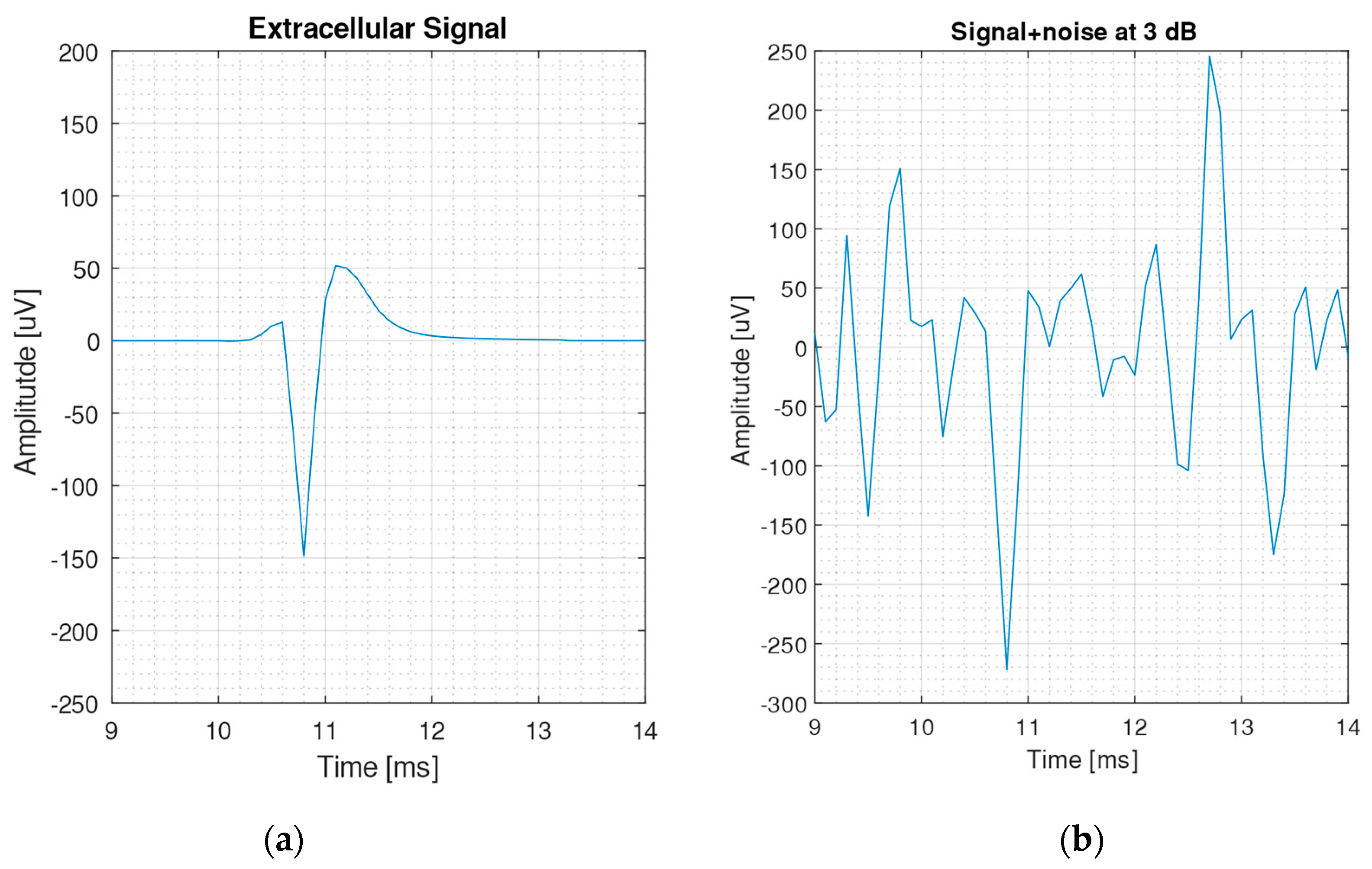
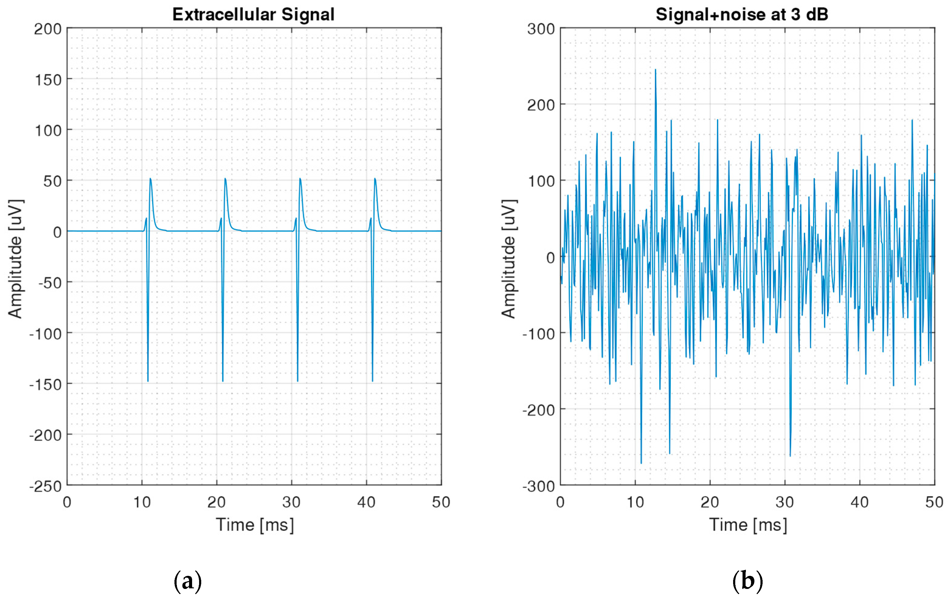
2.2. Generation of Neural Signals

The algorithms were tested on signal created using Neurocube, a tool for the generation of realistic simulation of extracellular recordings using detailed neuron models. The generated signal (Figure 2 shows 50 milliseconds activity of one channel) emulates a signal from an in vivo experiment where an array of seven honeycomb channels records the activity of a neuron spaced by 8.5 µm from the center of the array surface, plus other “far” neurons placed randomly in a cubic volume of 0.25 mm length above the sensor. The sampling frequency of each channels is set to 10 kHz, while the pixel size is set to 6 µm, spaced by 2 µm. Both sizes and sample rate lay in the range of the current MTA recording system characteristic. The neurons density is set to 300,000 neurons/mm², with 10% active neurons firing at 100 Hz. The entire record is 30,000 samples, corresponding to a 3 s duration for a total of 299 spikes. The synthetic dataset representing the noiseless electrical activity of the neural network is initially generated. Then, thermal noise is added to the dataset to allow for observations of the accuracy at different SNR levels. From the synthetic dataset, 10 datasets were obtained by adding the thermal noise at 21 different SNR levels (from −10 to 10 dB). Each algorithm was tested on all datasets and the results for each SNR level were averaged.

2.3. Spike Detection Algorithms

Three of the most used algorithms for spike detection, i.e., threshold crossing, the correlation-based algorithm, and the smoothed nonlinear energy operator (SNEO), were chosen for the comparison. Their performances are assessed through an FoM as introduced in Section 2.1. These methods were adapted to take advantage of the signal correlation provided by the high spatial resolution to find spikes even in the case of very poor SNR, since it is expected to sense the deterministic event of a spike simultaneously on all the pixels surmounted by a neuron, drowned in a mostly uncorrelated thermal noise. The first step is common for all these methods and consists of filtering of the raw signal with a second order passband Butterworth with a cutoff at 300 and 3000 Hz. Thus, from here onwards, the signal is defined as a filtered signal.

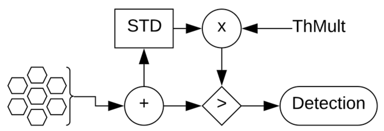
2.3.1. Threshold Crossing

Threshold crossing is the simplest and hardware-friendliest method between the three chosen spike detection algorithms. It consists of a comparison between the peaks of the filtered signal and a threshold. The comparison of the positive or the negative signal peaks is chosen depending on the most preponderant one in the spike shape. To conduct a fair comparison with the other two methods that exploit the spatial correlation of the activity, the filtered signal of the 7 pixels is summed and compared with a threshold dependent on the standard deviation of the sum, as shown in the block diagram in Figure 3.

The algorithm was optimized to achieve the best performances. For this method, the only parameter that can be varied is the threshold value. Figure 4 shows the results of accuracy using different threshold multipliers varying the SNR level. The threshold was set to recognize the negative peak of the spike, with a value of −2 times the noise standard deviation σ, a value that demonstrates the best performance in detection accuracy. The accuracy in the case of −1σ is seems to be higher for lower SNR (<2 dB), but it presents a tremendous number of FPs that makes the threshold unusable.

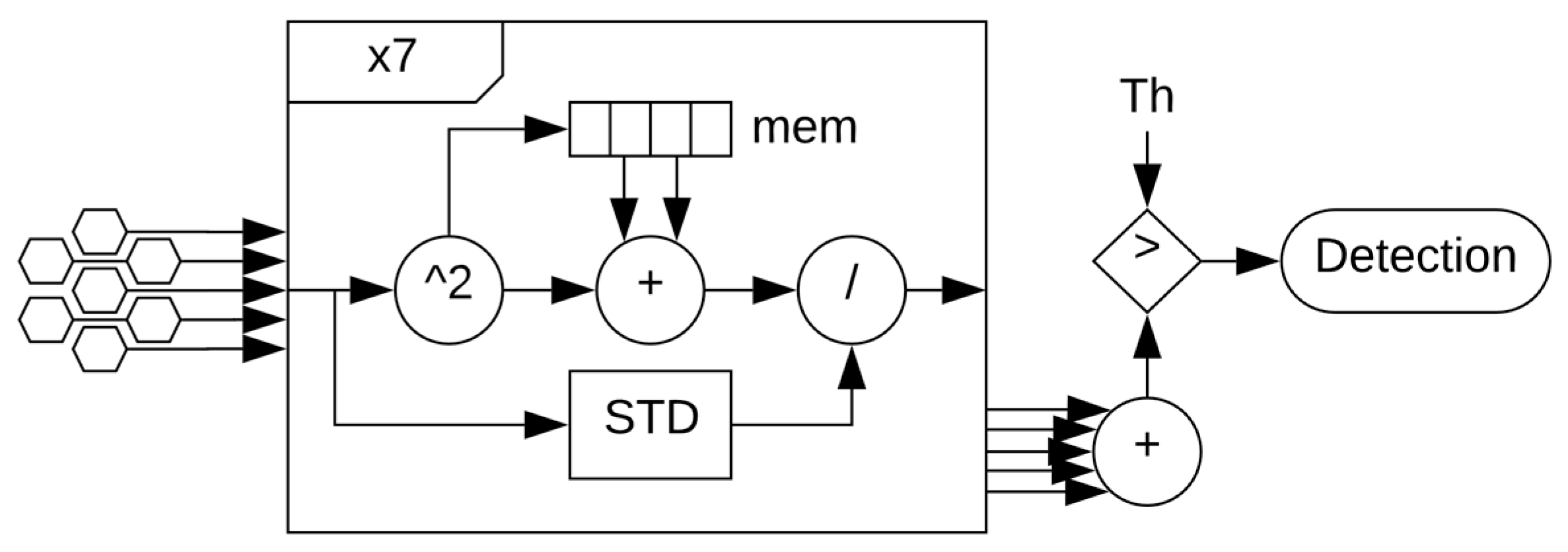
2.3.2. Correlation Algorithm

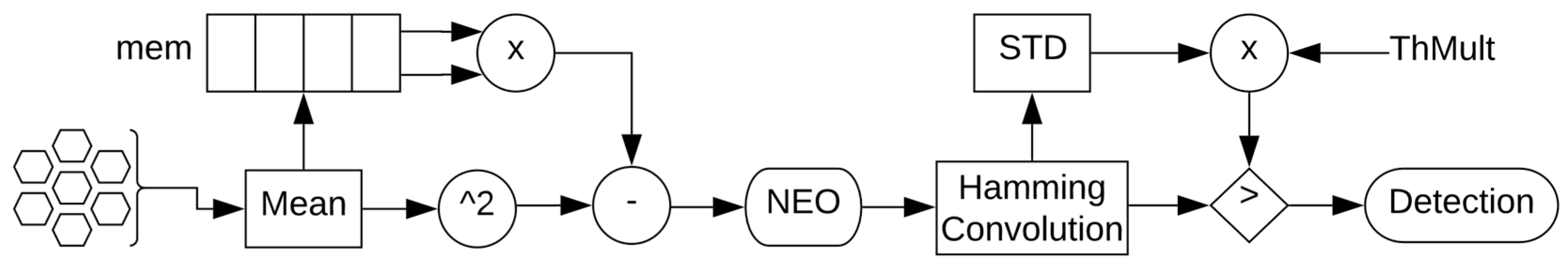
The Correlation algorithm searches for an equivalent pixel using both consecutive samples in time and adjacent pixels in space. In the implementation presented in [12], it exploits the temporal oversampling by summing three consecutive squared samples $v_p{}^2$ for each channel, but we tested the accuracy level using different temporal sum lengths. After the temporal sum, the algorithm then normalizes these values by each pixel standard deviation ${\sigma }_p^2$, to assign it a reliability. Every channel value is then summed with that of its six surrounding neighbors and is compared with a fixed, precomputed threshold $ThMult$, as explained in [12], to achieve one false positive per second on the 7-pixel group. The process is summarized in Equation (3), where N is the number of samples used for the temporal sum, and it is shown in Figure 5.

$$CA\left(v_p\left(\mathrm{n}\right)\right)={\displaystyle \sum }_{p=1}^7\frac{{{\displaystyle \sum }}_{\mathrm{k}=0}^{N-1}{v}_p{\left(n-k\right)}^2}{{\sigma }_p^2},$$

(3)

Figure 6 shows the results, where the better accuracy, in our simulations, is achieved without summing any consecutive temporal sample. Note that an accuracy over 99% is not reached by design, since the threshold is estimated and empirically adjusted to allow for a single false positive per second.

2.3.3. SNEO

The smoothed nonlinear energy operator (SNEO) gives an instantaneous estimation of the energy contained in a signal oscillation. Due to its energy answer, it has been proved to fit well the detection of spikes. This algorithm strictly depends on a parameter called $k$, which in turn depends on the sampling frequency and the average spike duration. After computing the nonlinear energy response (NEO block) of the signal samples, the SNEO soothes it using a Hamming window $w\left(4k+1\right)$ with a size of $4k+1$ and compares the result with a threshold multiple of the standard deviation of the output. Even in this case, the spatial correlation is exploited. In fact, as an input of this operator, the average of the 7-pixel group is considered. The operator is described in Equation (4) and shown in Figure 7.

$$SNEO=NEO\otimes w\left(4k+1\right),NEO\left(x\left(n\right)\right)=x{\left(n\right)}^2-x\left(\mathrm{n}+k\right)·x\left(\mathrm{n}-k\right),\mathrm{x}\left(n\right)={\displaystyle \sum }_{p=1}^7\frac{v_p\left(n\right)}{7}$$

(4)

The performance was tuned changing the $k$ parameter. Figure 8 shows the different performances of this operator testing $k$ at different SNR level. With greater $k$ value, the accuracy increases at a higher SNR level due to the reduced false positive amount, but the best tradeoff at the medium level SNR is achieved with $k=2$, where other widths are too conservative.

3. Results

The algorithms’ performances were evaluated on synthetic datasets described in Section 2.2. For each SNR level, 10 datasets were created. The performances measured for each algorithm at each SNR level are the average of the 10 results achieved on these datasets.

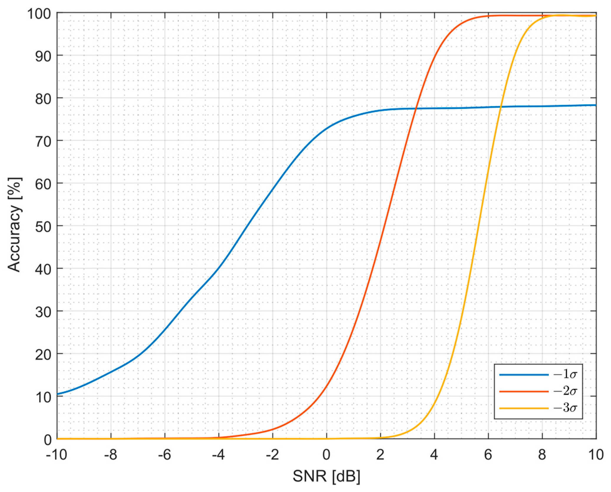
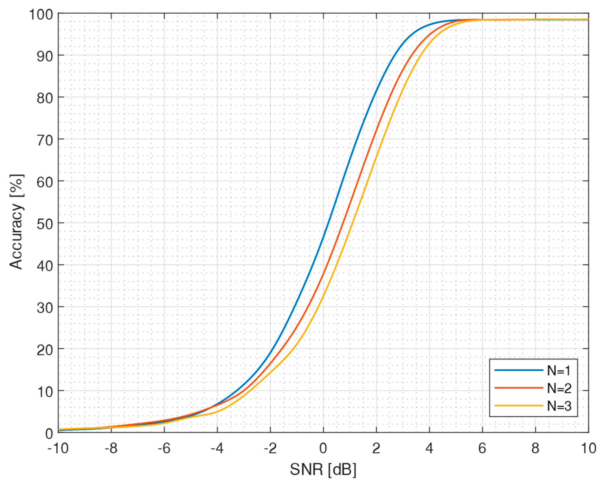
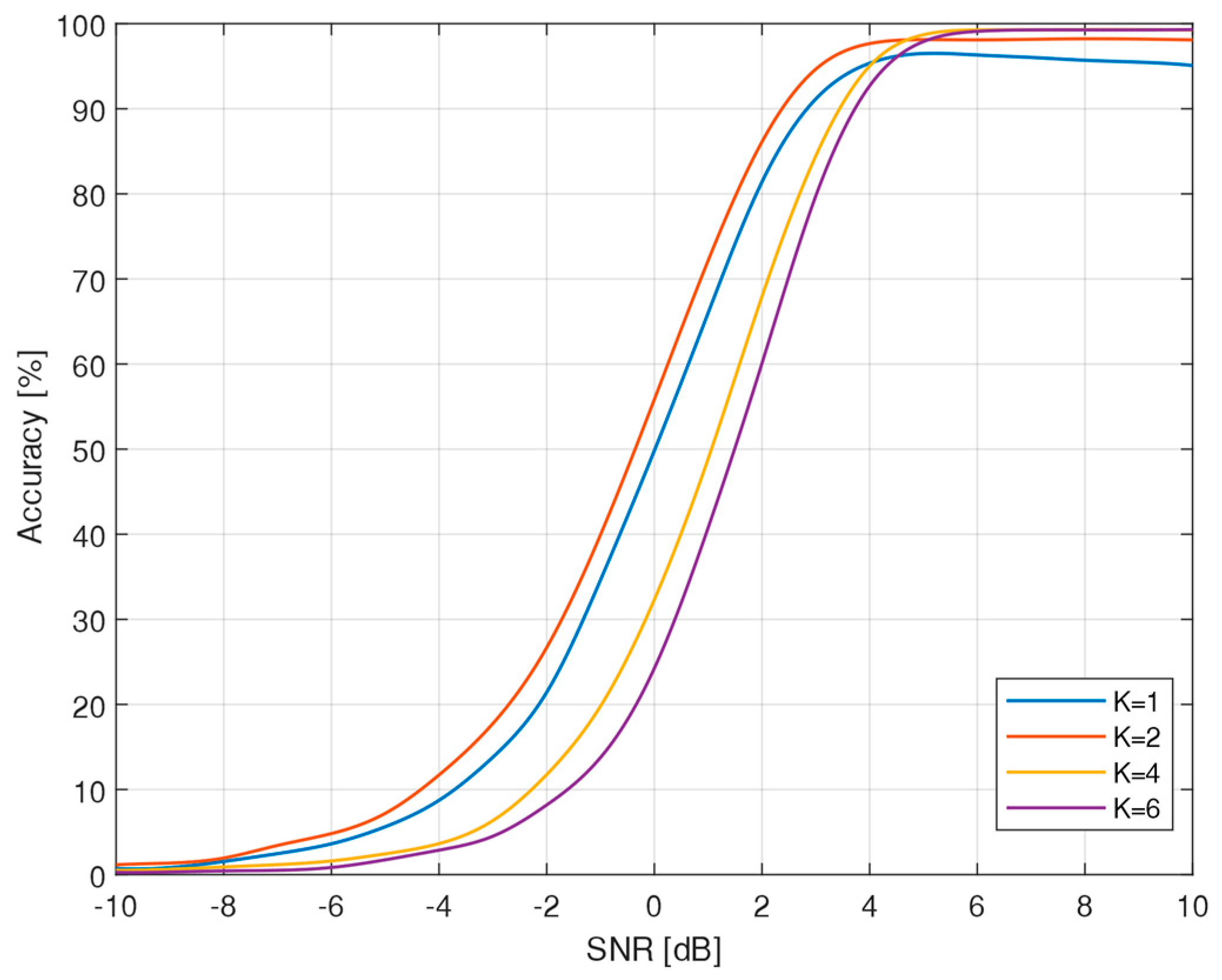
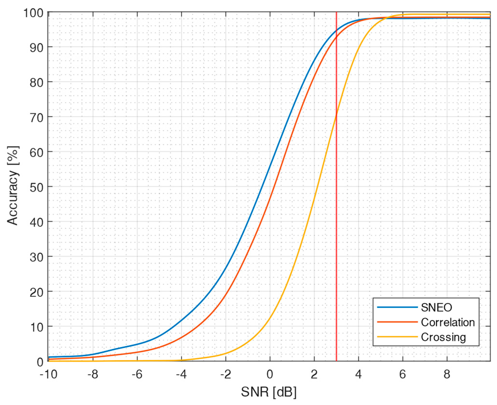
3.1. Algorithm Accuracy

The accuracy was estimated for each algorithm depending on the detection performances of true and false positives at 3 dB SNR as explained in Section 2.1, and Figure 9 shows the results. The SNEO detector provides the best detection accuracy from the lowest SNR level, followed by the correlation algorithm. The threshold crossing method requires from 2 to 4 dB SNR to achieve the same results as the others, but it also achieves 2–3% more accuracy from 5 dB SNR.

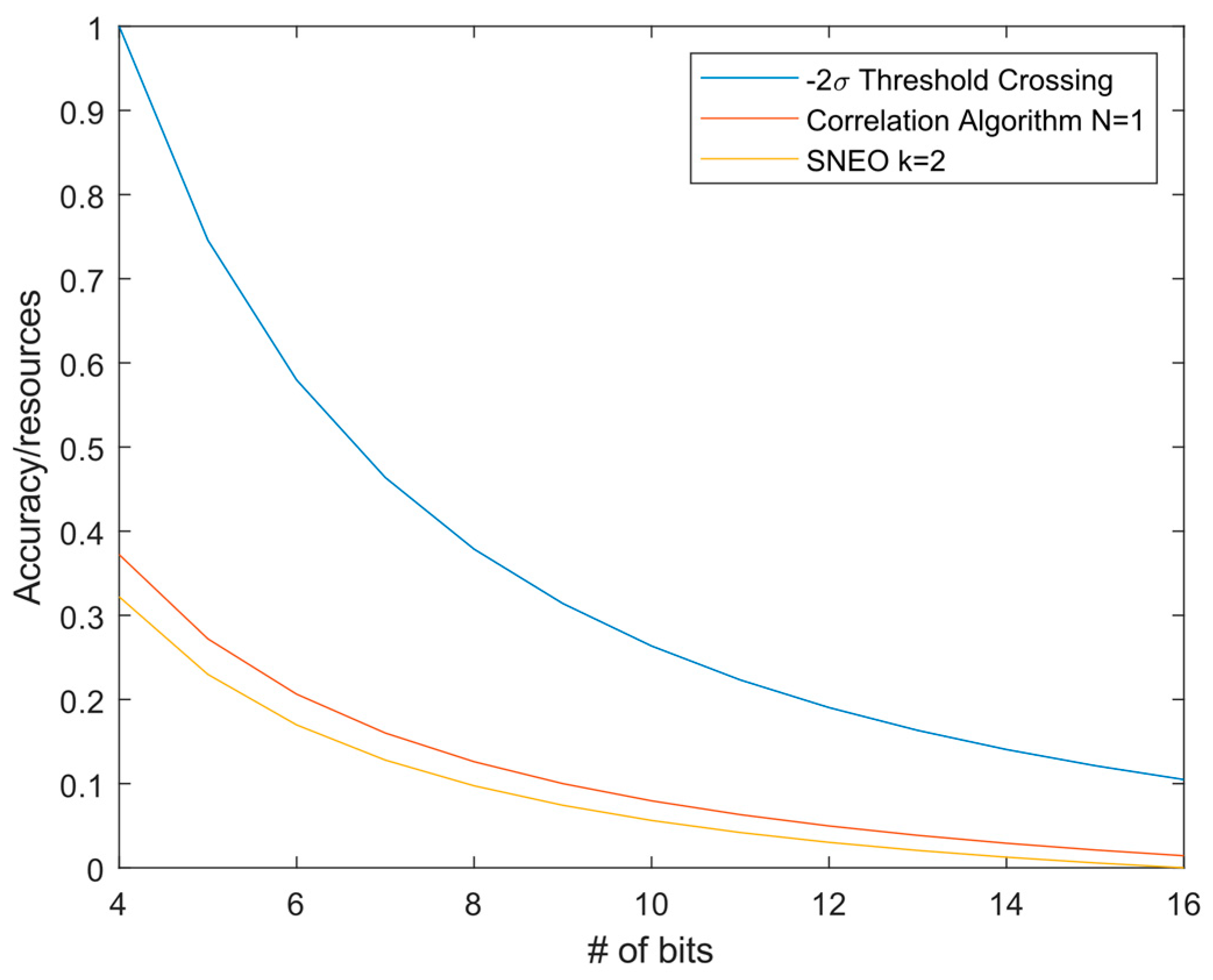
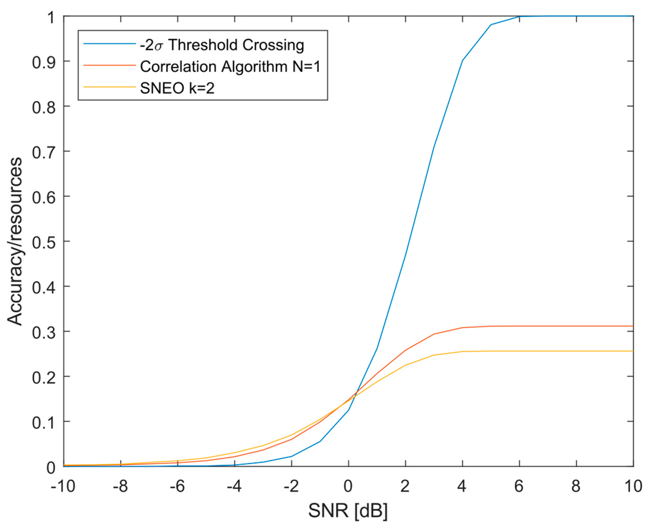
3.2. Resource Consumption

As introduced in Section 2.1, resource consumption is estimated as the amount of operations required by each algorithm. The filtering operation is common to all the spike detection methods and is considered once for each algorithm during the FoM evaluation. Each method requires the estimation of the standard deviation (STD) of the signal or of its output, computed as in Equation (5). The mean µ is assumed 0 as a consequence of the high-pass filtering of the data. The STD can be estimated over a power of 2 number of samples, allowing us to perform the division as a bit-shift operation, reducing the required resources.

$$STD=\sqrt{\frac{1}{N}{\displaystyle \sum }_{n=1}^{N}x{\left(n\right)}^2-\mathsf{\mu }},where\mathsf{\mu }\approx 0$$

(5)

For each operation, the logic gate amount is estimated, in detail (including operational pre-registers): adder is $23N$, multiplicator is $18N+6N^2$, comparator is $25N$, divisor is $28N$ and other registers are $9N$ logic gates each. $N$ is the number of the operand bits. Each operation is assumed in the integer domain—division included—and in a canonical form. For each operation, different algorithms exist, varying the amount of logic gates required, especially in implementation exploiting resource reutilization. Hopefully, the tradeoff between operation complexity and clock frequency in the case of resource reutilization leads to approximately comparable power consumption. For this reason, even if these resource estimation can be subjected to variation depending on the implementation, it can be considered sufficiently accurate to perform algorithm comparison.

Table 1. Resources required by the hardware implementation of the algorithms.

	Filter	Standard Deviation	Threshold Crossing	Correlation Algorithm	SNEO
Adder	4	1 + 1 1	6	20 1	1 + 6 1 + (4 k) 2
Multiplicator	5	1	2 *	3 + 2 *	2 + (4 k + 1) 1 + 2 *
Comparator	0	1	1	1 2	1 2
Divisor	0	0	0	7	0
Register	4 1	1 1	0	21 1	2 k + (4 k + 1) 1
STD	0	-	1	7	1
Weighted Total	254 N + 30 N 2	121 N + 6 N 2	235 N + 6 N 2 + STD	995 N+42 N 2 + 7 * STD	557 N + 602 kN + 36 N 2 + 48 kN 2 + STD 1
5-bit, k = 2	2020	755	2080	11,310	13,615
8-bit, k = 4	3952	1352	3616	20,112	25,240

¹ the operation occurs after a multiplication and it is weighted as $2N$. ² the operation occurs after two multiplications and it is weighted as $4N$. * one is for the threshold computation; one is to avoid the STD square root.

shows the resource estimation results for every considered algorithm.

4. Discussion

From the accuracy performance and resource consumption of each algorithm shown in Section 3.1 and Section 3.2, we can finally observe the FoM results in Figure 10. The curves show the ratio between the accuracy at 3 dB of SNR and the resources required for algorithm implementation with different sample widths. Detailed results are shown in

Table 2. Algorithm performances at 3 dB SNR.

	Threshold Crossing	Correlation Algorithm	SNEO
True Positive (%)	73	93	96
False Positive (%)	4	1	2
Accuracy (%)	70	93	95
Resources (8 bit)	3616	20,320	41,016
FoM (3 dB)	0.40	0.12	0.10

.

As can be observed, according to the FoM, the threshold crossing method outperforms by a factor of about 2.5× the others two algorithms, despite its poor accuracy, due to its light footprint in logic gate requirements (5× and 8× compared to SNEO and the correlation algorithm, respectively). Despite this consideration, a real winner must be chosen carefully, strictly depending on the scenario where the detector must lay. If there are tight constrains on power that can be provided to the circuit, the threshold crossing approach must be preferred, considering also that if the transmission bandwidth allows it, it is possible to sacrifice the accuracy lowering the threshold multiplier. A more relaxed threshold causes a higher number of FP, but it also increases the correct detections, as shown in the case of the threshold set to −σ in Figure 4; an external sorting/clustering of the detected spikes eventually discards the FP in the second step without a power constraint.

These considerations change for SNR above 4–5, as can be seen in Figure 9, where the threshold crossing method can be considered the best approach without exception, providing over 90% accuracy, and having 3–4× higher FoM than the competitors. Conversely, as shown in Figure 11, in the case of SNR lower than 1, the threshold crossing method lose its supremacy due to the very poor performances achieved. Here, the correlation and the SNEO algorithms can be considered equivalent in appearance of the FoM. Paying about 1.2× more logic gates when compared to the correlation algorithm, the SNEO clearly provides the better performances, with 5–7% better accuracy depending on the SNR. The $k$ parameter of the SNEO algorithm can considerably change the resource requirements of the algorithm, especially because of the convolution operation that makes the resources grow quadratically. However, for typical sampling frequency of up to 30 kHz, a $k$ lower than 6 should be sufficient for an accurate detection in most scenarios. A similar discussion can be applied where less constrained power limits are required; in fact, the better accuracy provided by these last two methods should be preferred over threshold crossing’s light footprint, at least below 5 dB of SNR. Results achieved under the 0 dB SNR level cannot surpass 50% accuracy with any of the proposed methods and are probably not suitable to extract relevant activity from the observed neuronal population. In this case, similarly to what was suggested with threshold crossing, the SNEO algorithm with a relaxed threshold and an off-the-MTA-chip processing step can help to increase the detections but, as consequence, the algorithm requires that both are paid more resources and that a greater amount of data is transmitted.

As a side note, the sample number of bits alone has appeared incapable of changing the consideration drawn until now, since it does not vary the relative distance of the algorithms in the FoM. As a general hint, a small quantization step—and so wider data samples in a bit—cannot carry any useful information about the signal depending on the SNR level. This reduces the FoM of each algorithm, increasing the resources required by each operation without bringing any advantages. It is possible to define a typical samples bit range laying under 8–10 bits, but the literature present different methods that allow one to improve the analog to digital converter (ADC) performances in power-constrained applications [17], lowering the required bit number without losing precision.

5. Conclusions

This paper focused on the accuracy and resource consumption of spike detection methods that are suitable for an in vivo low-power implantable MTA sensor, depending on the signal quality and available power. With an SNR over 4 dB, the threshold crossing method can provide good performances and is easily preferred over the more complex method. In the case of lower SNR (<2), the SNEO algorithm provides the absolute better detection accuracy between the compared methods.

References

1. Thewes, R.; Bertotti, G.; Dodel, N.; Keil, S.; Schroder, S.; Boven, K.-H.; Zeck, G.; Mahmud, M.; Vassanelli, S. Neural tissue and brain interfacing CMOS devices—An introduction to state-of-the-art, current and future challenges. In Proceedings of the 2016 IEEE International Symposium on Circuits and Systems (ISCAS), Montreal, QC, Canada, 22–25 May 2016; pp. 1826–1829. [Google Scholar] [CrossRef]
2. Hutzler, M.; Fromherz, P. Silicon chip with capacitors and transistors for interfacing organotypic brain slice of rat hippocampus. Eur. J. Neurosci. 2004, 19, 2231–2238. [Google Scholar] [CrossRef] [PubMed]
3. Schröder, S.; Cecchetto, C.; Keil, S.; Mahmud, M.; Brose, E.; Dogan, O.; Bertotti, G.; Wolanski, D.; Tillack, B.; Schneidewind, J.; et al. CMOS-compatible purely capacitive interfaces for high-density in-vivo recording from neural tissue. In Proceedings of the 2015 IEEE Biomedical Circuits and Systems Conference (BioCAS), Atlanta, GA, USA, 22–24 October 2015; pp. 1–4. [Google Scholar] [CrossRef]
4. Jang, H.-J.; Cho, W.-J. High performance silicon-on-insulator based ion-sensitive field-effect transistor using high-k stacked oxide sensing membrane. Appl. Phys. Lett. 2011, 99, 043703. [Google Scholar] [CrossRef]
5. Vassanelli, S.; Mahmud, M.; Girardi, S.; Maschietto, M. On the Way to Large-Scale and High-Resolution Brain-Chip Interfacing. Cogn. Comput. 2012, 4, 71–81. [Google Scholar] [CrossRef] [Green Version]
6. Eversmann, B.; Jenkner, M.; Hofmann, F.; Paulus, C.; Brederlow, R.; Holzapfl, B.; Fromherz, P.; Merz, M.; Brenner, M.; Schreiter, M.; et al. A 128 × 128 cmos biosensor array for extracellular recording of neural activity. IEEE J. Solid-State Circuits 2003, 38, 2306–2317. [Google Scholar] [CrossRef]
7. Voelker, M.; Fromherz, P. Signal Transmission from Individual Mammalian Nerve Cell to Field-Effect Transistor. Small 2005, 1, 206–210. [Google Scholar] [CrossRef]
8. Girardi, S.; Maschietto, M.; Zeitler, R.; Mahmud, M.; Vassanelli, S. High resolution cortical imaging using electrolyte-(metal)-oxide-semiconductor field effect transistors. In Proceedings of the 2011 5th International IEEE/EMBS Conference on Neural Engineering, Cancun, Mexico, 27 April–1 May 2011; pp. 269–272. [Google Scholar] [CrossRef]
9. Lewicki, M. A review of methods for spike sorting: The detection and classification of neural action potentials. Netw. Comput. Neural Syst. 1998, 9, R53–R78. [Google Scholar] [CrossRef]
10. Lambacher, A.; Vitzthum, V.; Zeitler, R.; Eickenscheidt, M.; Eversmann, B.; Thewes, R.; Fromherz, P. Identifying firing mammalian neurons in networks with high-resolution multi-transistor array (MTA). Appl. Phys. A 2011, 102, 1–11. [Google Scholar] [CrossRef] [Green Version]
11. Vallicelli, E.A.; Reato, M.; Maschietto, M.; Vassanelli, S.; Guarrera, D.; Rocchi, F.; Collazuol, G.; Zeitler, R.; Baschirotto, A.; De Matteis, M. Neural Spike Digital Detector on FPGA. Electronics 2018, 7, 392. [Google Scholar] [CrossRef] [Green Version]
12. Tambaro, M.; Vallicelli, E.A.; Tomasella, D.; Baschirotto, A.; Vassanelli, S.; Maschietto, M.; De Matteis, M. A 10 MSample/Sec Digital Neural Spike Detection for a 1024 Pixels Multi Transistor Array Sensor. In Proceedings of the 2019 26th IEEE International Conference on Electronics, Circuits and Systems (ICECS), Genoa, Italy, 27–29 November 2019; pp. 711–714. [Google Scholar] [CrossRef]
13. Mukhopadhyay, S.; Ray, G.C. A new interpretation of nonlinear energy operator and its efficacy in spike detection. IEEE Trans. Biomed. Eng. 1998, 45, 180–187. [Google Scholar] [CrossRef] [PubMed]
14. Ng, A.K.; Ang, K.K.; Guan, C.; Guan, C. Automatic selection of neuronal spike detection threshold via smoothed Teager energy histogram. In Proceedings of the 2013 6th International IEEE/EMBS Conference on Neural Engineering (NER), San Diego, CA, USA, 6–8 November 2013; pp. 1437–1440. [Google Scholar] [CrossRef]
15. Choi, J.H.; Jung, H.K.; Kim, T.; Taejeong, K. A New Action Potential Detector Using the MTEO and Its Effects on Spike Sorting Systems at Low Signal-to-Noise Ratios. IEEE Trans. Biomed. Eng. 2006, 53, 738–746. [Google Scholar] [CrossRef] [PubMed]
16. Kim, D.; Kung, J.; Chai, S.; Yalamanchili, S.; Mukhopadhyay, S. Neurocube: A Programmable Digital Neuromorphic Architecture with High-Density 3D Memory. In Proceedings of the 2016 ACM/IEEE 43rd Annual International Symposium on Computer Architecture (ISCA), Seoul, Korea, 18–22 June 2016; pp. 380–392. [Google Scholar] [CrossRef]
17. Hirai, Y.; Matsuoka, T.; Tani, S.; Isami, S.; Tatsumi, K.; Ueda, M.; Kamata, T. A Biomedical Sensor System with Stochastic A/D Conversion and Error Correction by Machine Learning. IEEE Access 2019, 7, 21990–22001. [Google Scholar] [CrossRef]
Figure 1. (a) A simulated extracellular spike template. (b) Spike template with noise at 3 dB signal-to-noise ratio (SNR).
Jlpea 10 00026 g001
Figure 2. (a) Fifty milliseconds of extracellular simulated activity without noise on a single channel of a pyramidal neuron generated by Neurocube. (b) Noisy dataset created from the noiseless template adding white noise to achieve an SNR of 3 dB.
Jlpea 10 00026 g002
Figure 3. Threshold crossing block diagram. STD represents the signal standard deviation calculation, while ThMult is the constant by which the standard deviation is multiplied to find the comparison threshold.
Jlpea 10 00026 g003
Figure 4. Threshold crossing accuracy using −σ, −2σ and −3σ as threshold values.
Jlpea 10 00026 g004
Figure 5. Correlation algorithm block diagram. Mem block defines a memory containing the last three samples for each channel, STD block computes the standard deviation of the square of the signal, and ThMult is the threshold used for the output comparison.
Jlpea 10 00026 g005
Figure 6. Correlation algorithm accuracy with a temporal summation of two and three samples and without summation (N = 1), where N is the number of summed samples.
Jlpea 10 00026 g006
Figure 7. Smoothed nonlinear energy operator (SNEO) blocks diagram. Mem contains the last 2 × k + 1 samples, and STD block and ThMult are used to estimate the threshold for an SNEO detection.
Jlpea 10 00026 g007
Figure 8. SNEO accuracy using different k values.
Jlpea 10 00026 g008
Figure 9. Algorithm accuracy (averaged) at different SNR levels. The red vertical line corresponds to 3 dB. Threshold crossing has a threshold of 2∙σ, the correlation algorithm averages three samples in time and the SNEO has a k parameter of 2.
Jlpea 10 00026 g009
Figure 10. Figure of merit (FoM) of algorithms, ratio of accuracy at 3 dB of SNR and logic gates required for implementation with different width of samples bits.
Jlpea 10 00026 g010
Figure 11. FoM of algorithms, ratio of accuracy and logic gates required for 8-bit implementation at different SNR levels.
Jlpea 10 00026 g011