
A Numerical Study of a Submerged Water Jet Impinging on a Stationary Wall
by
 , ,
, ,
Bo Hu
1,2 ,
,
Hui Wang
3,
Jinhua Liu
1,
Yong Zhu
4,
Chuan Wang
1,3,*,
Jie Ge
5 and
Yingchong Zhang
4 1
International Shipping Research Institute, Gongqing Institute of Science and Technology, Jiujiang 332020, China
2
Department of Energy and Power Engineering, Tsinghua University, Beijing 100084, China
3
College of Hydraulic Science and Engineering, Yangzhou University, Yangzhou 225009, China
4
National Research Center of Pumps, Jiangsu University, Zhenjiang 212013, China
5
SHIMGE Pump Co., Ltd., Taizhou 317525, China
*
Author to whom correspondence should be addressed.
J. Mar. Sci. Eng. 2022, 10(2), 228; https://0-doi-org.brum.beds.ac.uk/10.3390/jmse10020228
Submission received: 30 December 2021
/
Revised: 30 January 2022
/
Accepted: 1 February 2022
/
Published: 8 February 2022
(This article belongs to the Section Ocean Engineering)
Abstract
:The impinging jet is a classical flow model with relatively simple geometric boundary conditions, and it is widely used in marine engineering. In recent years, scholars have conducted more and more fundamental studies on impact jets, but most of the classical turbulence models are used in numerical simulations, and the accuracy of their calculation results is still a problem in regions with large changes in velocity gradients such as the impact zone. In order to study the complex flow characteristics of the water flow under the condition of a submerged jet impacting a stationary wall, the Wray–Agarwal turbulence model was chosen for the Computational Fluid Dynamics (CFD) numerical simulation study of the impacting jet. Continuous jets with different Reynolds numbers and different impact heights H/D were used to impact the stationary wall, and the results show that the jet flow structure depends on the impact height and is relatively independent of the Reynolds number. With the increase in the impact height, the diffusion of the jet reaching the impact area gradually increases, and its velocity gradually decreases. As the impact height increases, the maximum pressure coefficient decreases and the rate of decrease increases gradually, and the dimensionless pressure distribution is almost constant. In this paper, the flow field structure and pressure characteristics of a continuous submerged jet impacting a stationary wall are explored in depth, which is of great guidance to engineering practice.
1. Introduction
A submerged impinging jet is a flow structure in which the fluid is shot out of the orifice or slit, enters the same medium, and impacts its solid wall, mixing with the ambient fluid [1]. At present, submerged impinging jets are widely used in marine engineering. Wang et al. [2] conducted an in-depth study of the application of water jet technology in solid fluidized extraction of marine natural gas hydrate (NGH) by designing orthogonal experiments and gave the spirit boundary breakage velocity for gas hydrate deposition. Liu et al. [3] proposed a new biomimetic antifouling method based on water jet for marine structures, and the experimental and numerical simulation results showed that the method is able to prevent the attachment of unicellular fouling organisms, thereby hindering the entire fouling process. In addition, submerged impinging jets are used in underwater cutting operations, subsea pipeline and cable laying [4,5,6], etc. Therefore, the study of submerged impinging jets is of great practical significance to the development of marine engineering and its affiliated industries. In order to provide theoretical support for engineering research, basic research on impinging jets is also essential. In recent years, many domestic and foreign scholars have conducted a large number of experimental and numerical simulation studies on impinging jets. JA Fitzgerald et al. [7] investigated the turbulent structure and impact zone of the impinging jets under two different nozzles using flow visualization and found that the size of the impact zone increases linearly with the impact distance and its size is independent of the jet Reynolds number. Abdel-Fattah et al. [8] used numerical calculations and experiments to study the impact of two-dimensional dual jets under different conditions, and the results showed that, as the jet angle increases, the stagnation point moves radially in the direction of the main flow, and the recirculation zone becomes wider. Hassan et al. [9] used time-resolved–particle image velocimetry (TR–PIV) technology and polarographic measuring instrument to study the influence of large-scale vortex structures on the shear stress of the circular impinging jet wall and found that the shear stress amplitude of the upstream wall increases, while the shear stress amplitude of the downstream recycling area decreases sharply, in the separation zone of the boundary layer. Charmiyan et al. [10] used tomography velocity measurement technology to conduct an experimental study on the slit impinging turbulent jet and found that the maximum turbulence intensity of the jet appeared in the shear layer, and there was an attenuation zone near the impact wall, and the turbulence intensity at the center of the jet gradually increases as it approaches the impact wall. Pieris et al. [11] used the TR–PIV technology to conduct an experimental study on the slit impinging jet produced by a nozzle with a high aspect ratio and found that the instability of the jet shear layer is the main reason for the primary vortex formed by the impinging jet, and the vortices merge near the impingement area. The secondary vortex is caused by the interaction between the merged primary vortex and the wall, and its formation frequency is a quarter of the primary vortex shedding frequency. Markal et al. [12] studied the hydrodynamic and thermal characteristics of coaxially confined impinging jets through experiments and found that increasing the ratio of impact distance to Reynolds number can significantly improve the uniformity of heat transfer. Zhang et al. [13] used the Wray–Agarwal turbulence model to study the unsteady flow characteristics of the pulsed jet impinging on the rotating wall and found that the radial distribution of the velocity near the jet outlet gradually became non-uniform over time and, finally, coincided with the velocity at steady state. Xu et al. [14] used the Standard k–ε model, Re–Normalization Group (RNG) k–ε model with wall function, and the low Reynolds number k–ε model, to numerically simulate the impinging jet flow field of a semi-confined circular tube, and the results showed that the simulation errors of the standard k–ε model and the low Reynolds number k–ε model were too large, while the results of the RNG k–ε model were closer to the experimental data. Chen et al. [15] simulated and studied turbulent impinging jets, and after comparing them with the experimental results, it was found that the accuracy of the improved model calculation was significantly improved, especially for the prediction of the turbulent kinetic energy distribution in the stagnant region. Jiao et al. [16] used the standard k–ε model and the wall function method to numerically simulate the semi-enclosed flow field of a submerged liquid jet impacting a flat plate at different impact heights and found that the center of the return zone moved downstream as the impact height increased, while the distance from the impacting flat plate remained essentially constant.
From the establishment of mathematical models for theoretical studies [17,18,19,20,21,22,23,24,25] to quantitative analysis by high-precision experiments [26,27,28,29], the methods researchers use to solve scientific problems are constantly advanced. At the same time, the advancement of science and technology and the increasing sophistication of CFD technology [30] have brought great changes to the research methods of impinging jets. With the increasing accuracy of research results from simple experimental studies to experimental studies with high-precision testing techniques [31] and then to the combination of experimental studies and numerical calculations [32,33,34,35,36,37], the understanding of impinging jets has been deepened. However, there is still a certain deviation between the numerical calculation results and experimental results, especially in an impact area with a high-pressure gradient and rapid speed change. Therefore, it is very necessary to improve the accuracy of numerical calculations of impinging jets. In this paper, the Wray–Agarwal turbulence model, developed based on the k–ω model, is used to study the coupling flow of continuous jet impact on a static wall under flood conditions, and to analyze the flow field characteristics and impact pressure characteristics of the flow, which is of great significance to engineering practice. Table 1 briefly lists the turbulence models used in the existing literature and the extent to which they have been improved in this paper.
2. Modeling and Numerical Methods
2.1. Model Building
Figure 1 is a schematic diagram of a submerged jet impacting a stationary wall; the fluid was sprayed horizontally through a sufficiently long circular nozzle and impacted the wall of the stationary disk, forming the entire impinging jet flow field in the cylindrical water tank and finally flowed out through the gap between the stationary disk and the cylindrical water tank. The nozzle was perpendicular to the wall of the rotating disk, and its centerline coincided with the centerline of the disk. In order to better study the continuous jet impacting the stationary wall, a spatial right-angle coordinate system o1xyz was established. The coordinate origin o1 was the center of the disk, the z-axis was perpendicular to the disk wall, and the x-axis and y-axis were perpendicular to each other and parallel to the wall of the disk. In order to investigate the general law of impinging jets, the fluid domain above the disk was taken as the study object, and the size and spatial position of the model are dimensionless, with the inner diameter D of the nozzle. The inner diameter of the nozzle D = 10 mm, the outer diameter Dw = 12 mm, the radius of the cylindrical flume Rc = 25D (250 mm), and the radius of the stationary disk R = 15D (150 mm). The correctness of the numerical simulation model was verified by comparing the numerical simulation results of the axial distribution of the dimensionless velocity of the jet with the experimental results of the PIV.
2.2. Numerical Methods and Boundary Conditions
The jet flow field is a submerged impinging jet, and the jet medium is incompressible water. The solution was performed by the computational fluid dynamics software ANSYS FLUENT 19.2. The Reynolds–Averaged Navier–Stokes (RANS) method was chosen to solve the Reynolds stress term. The convective term was discretized in a second-order windward format. The pressure and velocity coupling adopted the SIMPLE–consistent (SIMPLEC) algorithm. The residuals of the final iterative results were less than 10−5, and the total number of iterative steps exceeded 20,000.
- (1)
- Inlet boundary: the nozzle inlet face was set up as a velocity inlet;
- (2)
- Outlet boundary: the outlet was far from the impact origin, and the turbulent flow reached relative equilibrium, so a pressure outlet was used;
- (3)
- Wall condition: the solid wall was set up as a non-slip wall surface.
2.3. Grid Independence Analysis
For the numerical calculation of impinging jets, compared with unstructured grids, structured grids have the advantages of easier fitting regional boundaries and more accurate simulation of flow details [38]. Therefore, the model was delineated with a hexahedral structured mesh using the professional commercial software ANSYS ICEM CFD 19.2 [39]. A hexahedral grid can effectively reduce the pseudo-diffusion caused by poor grid quality and can also improve the computational speed. The grid was encrypted near the impact wall where rapid changes in velocity and pressure occurred by controlling the number of grid nodes. It was ensured that the aspect ratio of the grid and the dimensions between adjacent grids would not differ significantly and that the angle was greater than 18° and less than 90°. The grid node spacing of the first layer on the impact wall was set to 0.1 and gradually increased in the ratio of 1.1 away from the impact wall, to realize the encryption of the boundary layer.
Theoretically, the denser the grid, the more accurate the computational results obtained. However, the grid cannot be encrypted indefinitely because the denser the grid is, the more computationally intensive the solution is, and the longer the computational cycle is, while our computational resources are limited. Additionally, as the grid is encrypted, the rounding error of the computer floating-point operation will increase, which requires us to find a more suitable number of grids that will neither lose accuracy considerably nor significantly consume computational resources. Figure 2 shows the average velocity of the cross-section in the jet at different grid sizes G. As the grid size G gradually decreases, the average velocity of the cross-section in the jet decreases as well; when the grid size G ≤ 2.5, the average velocity of the cross-section in the entire jet flow field remains essentially constant, which meets the requirement of grid independence [40,41,42]. Considering the coordination of computational accuracy and computer resources, G = 2.0 was selected to mesh the model, as shown in Figure 3. The total number of computational domain grids is 3,523,120, the number of nodes is 3,445,790, the minimum value of mass is 0.7, and the maximum value of y+ is 8.3.
2.4. Turbulence Model Verification
The Wray–Agarwal (W-A) turbulence model is a single-equation turbulence model established by the k–ε closed model [43]. The W–A turbulence model uses the ω equation with cross-diffusion terms, but also retains the link to the k–ε model, which improves the accuracy of predicting equilibrium flow and the ability to interpret non-equilibrium flow [44].
Vortex viscosity equation is defined as follows:
R is the transport equation as follows:
The presence of the two terms C2kω and C2kε makes the Wray–Agarwal turbulence model behave as a single-equation k–ω model or a single-equation k–ε model, with f1 as the switching function. f1 switching function is a modified version of the hybrid function used in the SST k–ω model described as follows:
where μτ denotes the viscosity of turbulence (Pa/s); ρ denotes the density of the fluid (kg/m3); fμ denotes the damping function; k represents the pulsating kinetic energy of turbulence (J); ω is the specific dissipation rate; ν is the kinematic viscosity (m2/s); d is the distance to the nearest wall (m).
In this numerical simulation study, six turbulence models—namely, BSL k–ω, SST k–ω, standard k–ε, RNG k–ε, realizable k–ε, and Wray–Agarwal, were selected to numerically calculate the jet impact on the stationary wall, and the calculated results were compared with the PIV experimental results (Re = 35,100, impact height H/D = 3).
Figure 4 shows the axial distribution of the dimensionless velocity V/Vj (Vj is the average velocity of the jet outlet) obtained from different turbulence model calculations and PIV experiments. As can be seen from the figure, in the free-jet region (1 ≤ z/D ≤ 3) (z is the vertical distance from the corresponding point to the impact wall), the dimensionless velocity V/Vj remains basically constant. Compared with other turbulence models, the dimensionless velocity V/Vj calculated by the Wray–Agarwal turbulence model is closer to the PIV experimental value. In the impact region (0 < z/D ≤ 1), the dimensionless velocity V/Vj decreases rapidly, and the calculated results of different turbulence models are relatively concentrated, which is in good agreement with the PIV experimental data. In a comprehensive comparison, it is found that the prediction results based on the Wray–Agarwal turbulence model fit better with the experimental results, so in this study, the Wray–Agarwal model was used for numerical simulation.
2.5. Nozzle Length Analysis
Within a certain distance, the fluid in the circular pipe flows, acting together with the influence of factors such as frictional resistance, and the velocity distribution on the same cross-section constantly changes. After the fluid develops for a certain distance, the thickness of the boundary layer gradually stabilizes, and the velocity distribution in the radial direction remains basically unchanged. At this time, the fluid flow in the circular pipe is considered to be fully developed. In order to avoid interference with the subsequent impinging jet flow due to the insufficient development of the circular pipe flow in the study, this section discusses the length of the circular pipe in the experiment that can make the turbulent flow fully developed.
2.5.1. Choice of Nozzle Length
The inlet of the circular pipe adopts the average velocity inlet (Re = 10,000), while the outlet is set as the pressure outlet (P = 1 atm). In order to better describe the fluid flow in the pipe (Figure 5), a rol coordinate system was established, with the center of the pipe inlet as the coordinate origin o, the radial direction as the r-axis, and the axial direction as the l-axis, taking the fluid flow direction as the positive direction.
Figure 5 shows the distribution nephogram of the dimensionless velocity V/Vj in the cross-section in a circular pipe of length 60D. As can be seen from the figure, with the flow of the fluid, the velocity of the fluid near the wall of the pipe decreases due to the viscous shear stress. The velocity of the main flow in the pipe first increases and then remains unchanged, and a high-speed core region appears. As the flow develops, the high-speed core region gradually narrows and then disappears; the high-speed core region arises at about L/D ≈ 10.5 and disappears at L/D ≈ 28. When L/D ≥ 30, the distribution of dimensionless velocity V/Vj on the cross-section of the pipe remains constant.
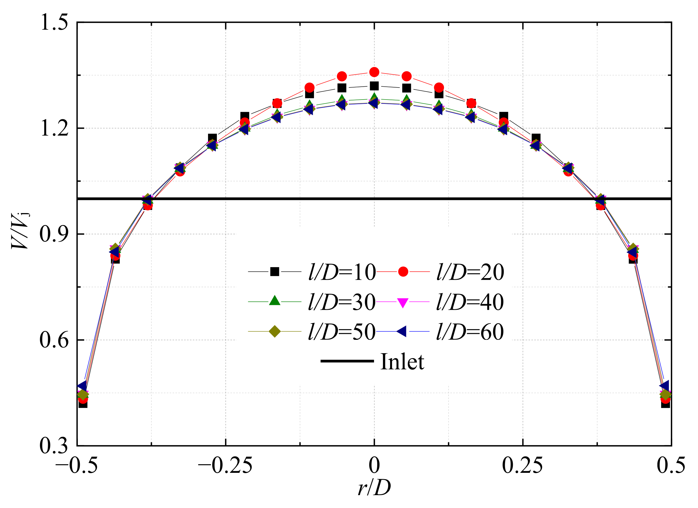
As shown in Figure 6, in order to quantify the development of turbulent flow along the pipe, the radial distribution of the dimensionless velocity V/Vj at different pipe positions was investigated. It can be seen from the figure that the maximum velocities at different axial positions of the circular pipe all appear on the axial center of the circular pipe (r/D = 0), and the radial distribution of V/Vj is symmetrical about the circular pipe axis. For the different pipe positions selected (l/D = 10, 20, 30, 40, 50, and 60), the maximum value of the pipe flow V/Vj appears at the center of the pipe with l/D = 20. After the fluid enters the circular tube, the fluid velocity near the wall (|r/D| ≥ 0.375) decreases rapidly, as the flow in the circular tube develops, and then remains constant, but the fluid velocity in the mainstream region (|r/D| ≤ 0.375) first increases, then decreases, and then remains unchanged; the closer to the center of the pipe, the greater the velocity increase. When L/D > 40, the radial distribution curves of the dimensionless velocity V/Vj coincide, indicating that the flow of the circular pipe is fully developed, and the magnitude of V/Vj at the same position remains constant.
2.5.2. Demonstration of the Full Development of Turbulence
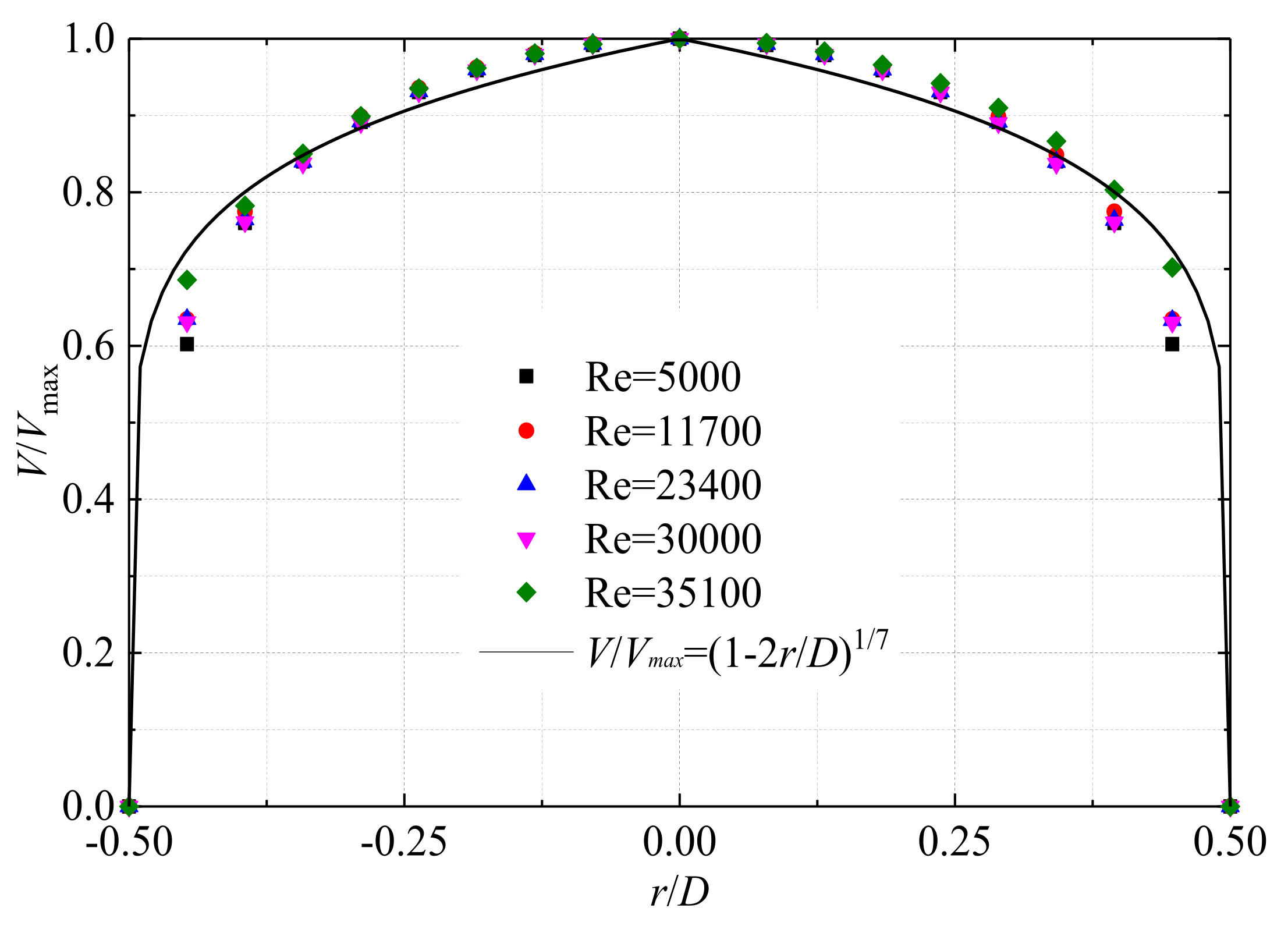
Through a large number of studies on the turbulent flow of a circular pipe, scholars at home and abroad have obtained an empirical formula for the radial distribution of the turbulent flow of a circular pipe, which is
In Equation (7), the 1/n power is used to describe the radial distribution of the velocity in the pipe. Cooper et al. [45] found that when n = 7, the empirical equation was able to describe approximately the radial distribution of turbulent flow velocities in a fully developed circular pipe.
Figure 7 shows the radial distribution of the dimensionless velocity V/Vmax at the outlet of the pipe under the conditions of different Reynolds numbers and L/D = 50 and compared with the above empirical formula of turbulent velocity distribution. It can be seen from the figure that, in the mainstream region (|r/D| ≤ 0.375), the radial distribution of V/Vmax at the outlet of the pipe under different Reynolds numbers is basically the same, and there is a certain deviation in the dimensionless velocity V/Vmax distribution near the wall under different Reynolds numbers. The larger the Reynolds number, the smaller the resistance of the laminar flow along the pipe, and the smaller the deviation of V/Vmax distribution. The radial distribution curve of the dimensionless velocity V/Vmax at the outlet of the circular pipe under different Reynolds numbers agrees well with the empirical formula for the turbulent velocity distribution of the fully developed circular pipe. Therefore, the circular pipe with L= 50D can ensure the full development of the turbulent flow under different Reynolds numbers.
3. Research on Continuous Jet Impacting on Static Wall
3.1. Flow Field Analysis of Impinging Jet
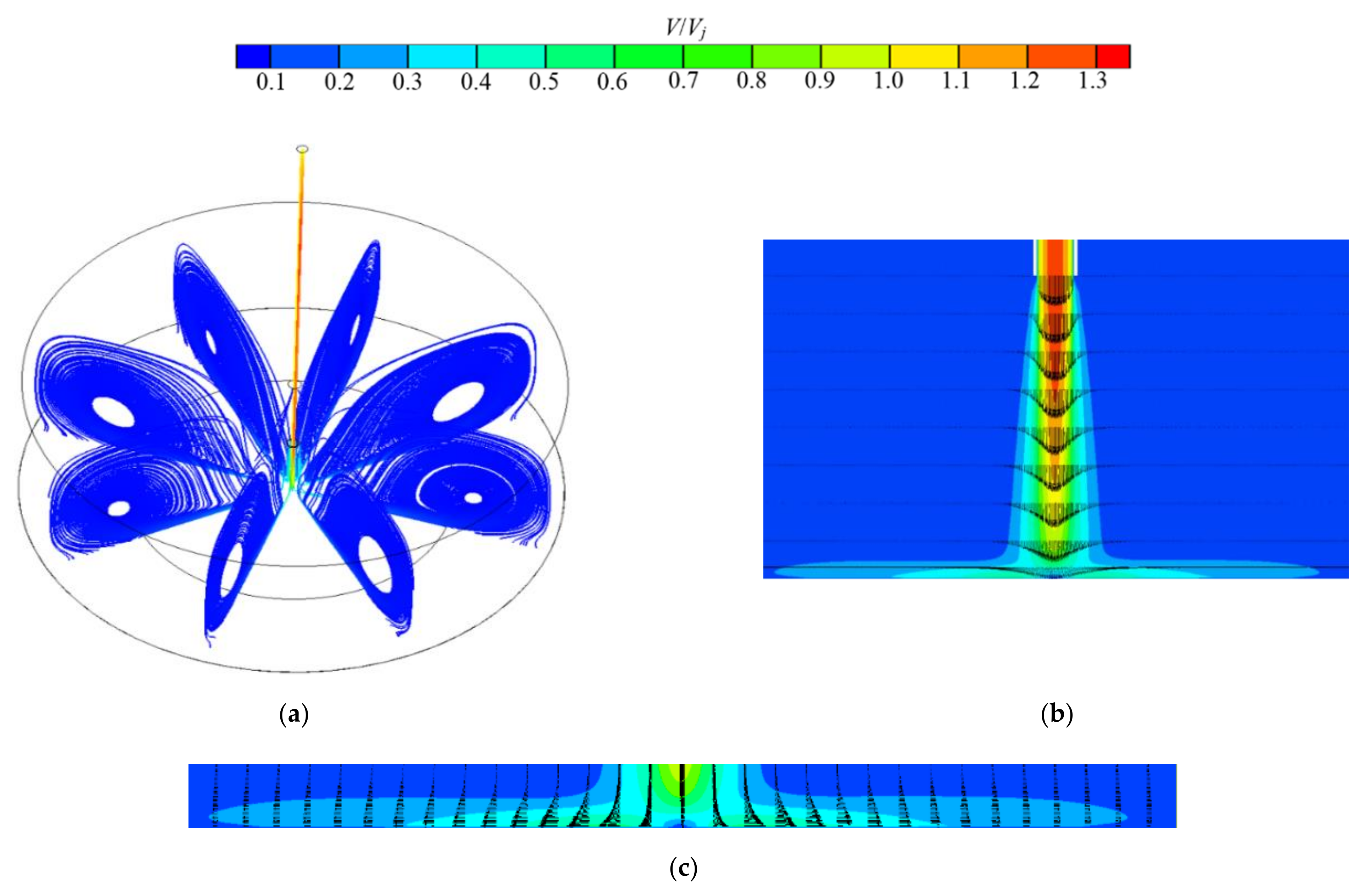
In order to better describe the jet’s flow field structure, the flow field structure of the jet’s full flow field under the conditions of impact height H/D = 8 and Reynolds number Re = 35,100 is given in Figure 8a–c, showing the velocity nephogram and vector diagram of the jet’s cross-section (on the xoz plane) and its near-wall region (0 ≤ z/D ≤ 1), respectively. It can be seen from Figure 8b that after the fluid is ejected from the nozzle, the diameter of the jet gradually increases, and the velocity gradually decreases, due to diffusion and entrainment of the surrounding fluid. From the velocity nephogram and vector diagram of the near-wall flow field in Figure 8c, it can be seen that after the fluid impacts the disk wall, the flow direction deflects radially, forming a wall jet parallel to the disk wall. The wall jet spreads radially in all directions to the vertical sidewall and is forced to turn again, eventually forming a huge recirculation zone on both sides of the jet in the two-dimensional plane and forming a vortex ring-like structure in the three-dimensional cylindrical flume, as shown in Figure 8a.
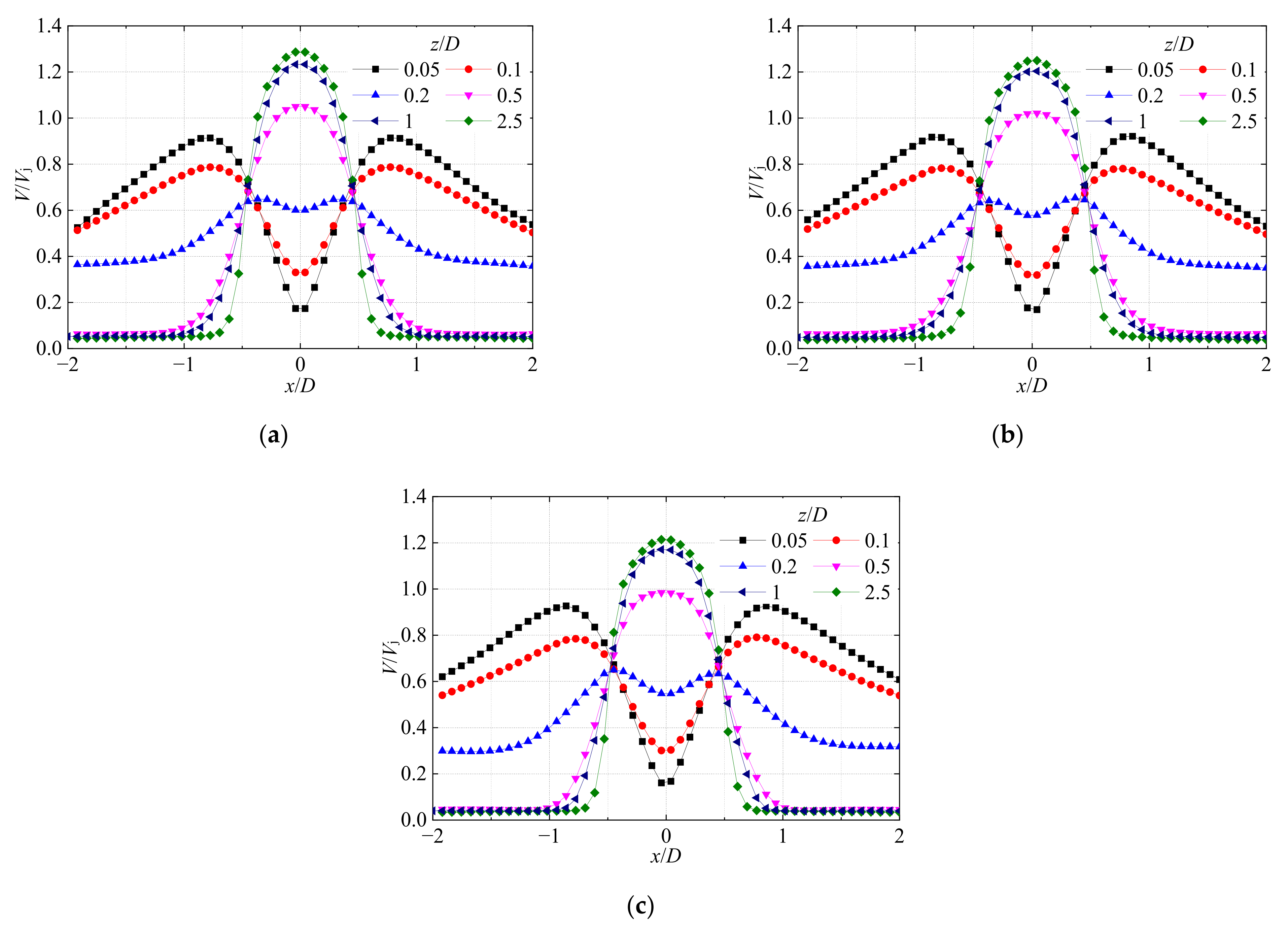
Figure 9 shows the distribution of the dimensionless velocity V/Vj along the radial direction x/D in the midsection (xoz plane) of the continuous jet impinging on the stationary wall jet with different Reynolds numbers and H/D = 3 conditions. It can be seen from the figure that, under the same Reynolds number, in the free-jet region (z/D ≥ 1), the radial distribution of the dimensionless velocity V/Vj varies less along the radial direction as the axial height z/D decreases; in the impact region (0 ≤ z/D ≤ 1), the radial distribution of the jet’s dimensionless velocity V/Vj changes greatly with the decrease in axial height z/D. When the Reynolds numbers are different, there is no significant change in the distribution of the dimensionless jet velocity V/Vj along the radial direction at the same axial height z/D. It is shown that, for a continuous jet impacting a stationary wall, at the same impact height, the jet flow structure is relatively independent of the Reynolds number.
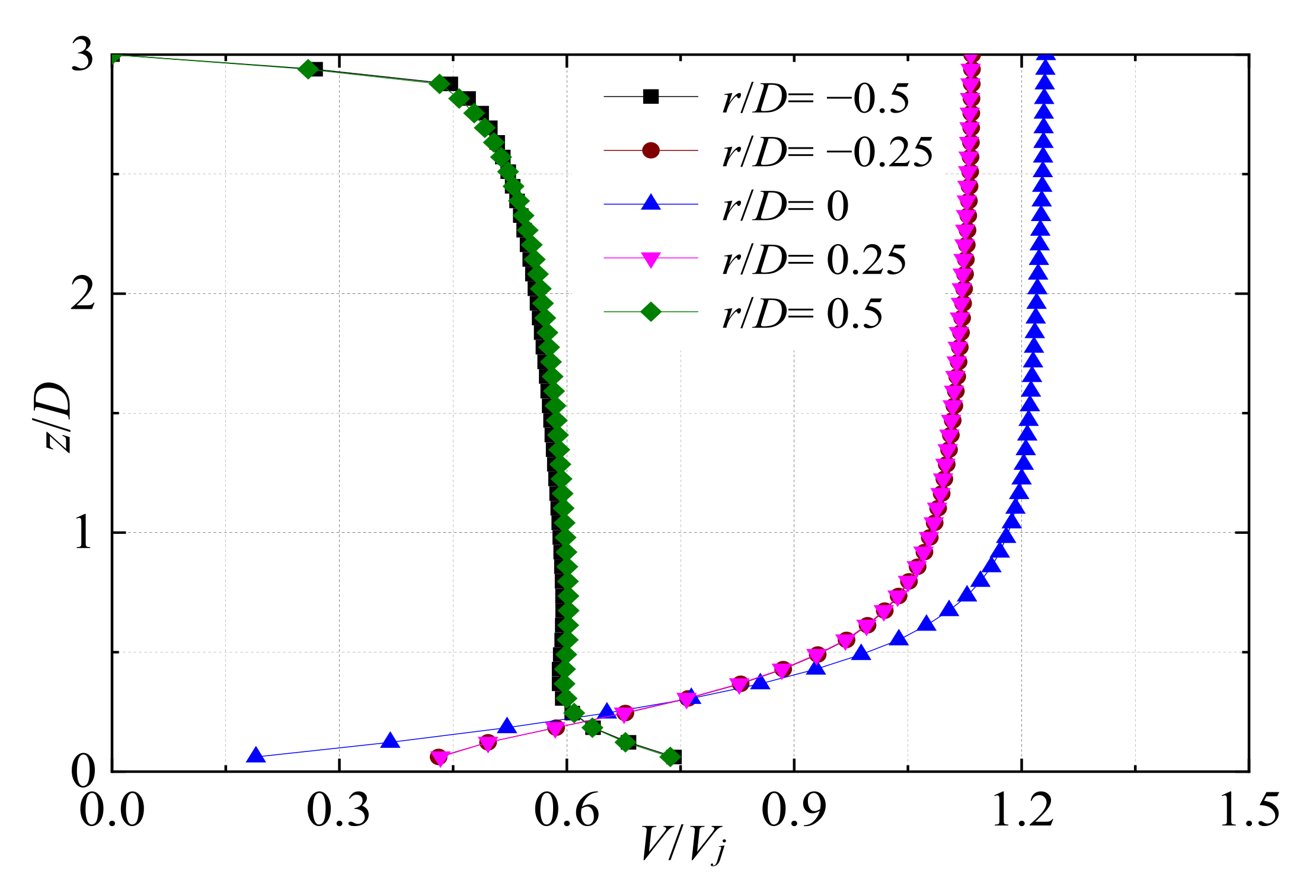
Figure 10 shows the axial distribution of the dimensionless velocity V/Vj at different radial positions of the cross-section in the continuous jet impacting the stationary wall jet under the conditions of impact height H/D = 3 and Reynolds number Re = 35,100. It can be seen from the figure that the axial distribution of the dimensionless velocity V/Vj at the radial position symmetrical about the jet center (r/D) completely coincides. When the radial position r/D = 0 or ±0.25, the dimensionless velocity V/Vj gradually decreases in the free-jet region (1 ≤ z/D ≤ 3) as the jet develops; it rapidly decreases in the impact region (0 ≤ z/D ≤ 1), and the magnitude of the decrease gradually increases. When the radial position r/D = ±0.5 (i.e., located in the shear layer between the jet and the ambient fluid), the dimensionless velocity V/Vj increases rapidly from 0 as the jet develops, and the increasing velocity decreases. The jet turns near the impact wall, and the dimensionless velocity V/Vj increases rapidly again.
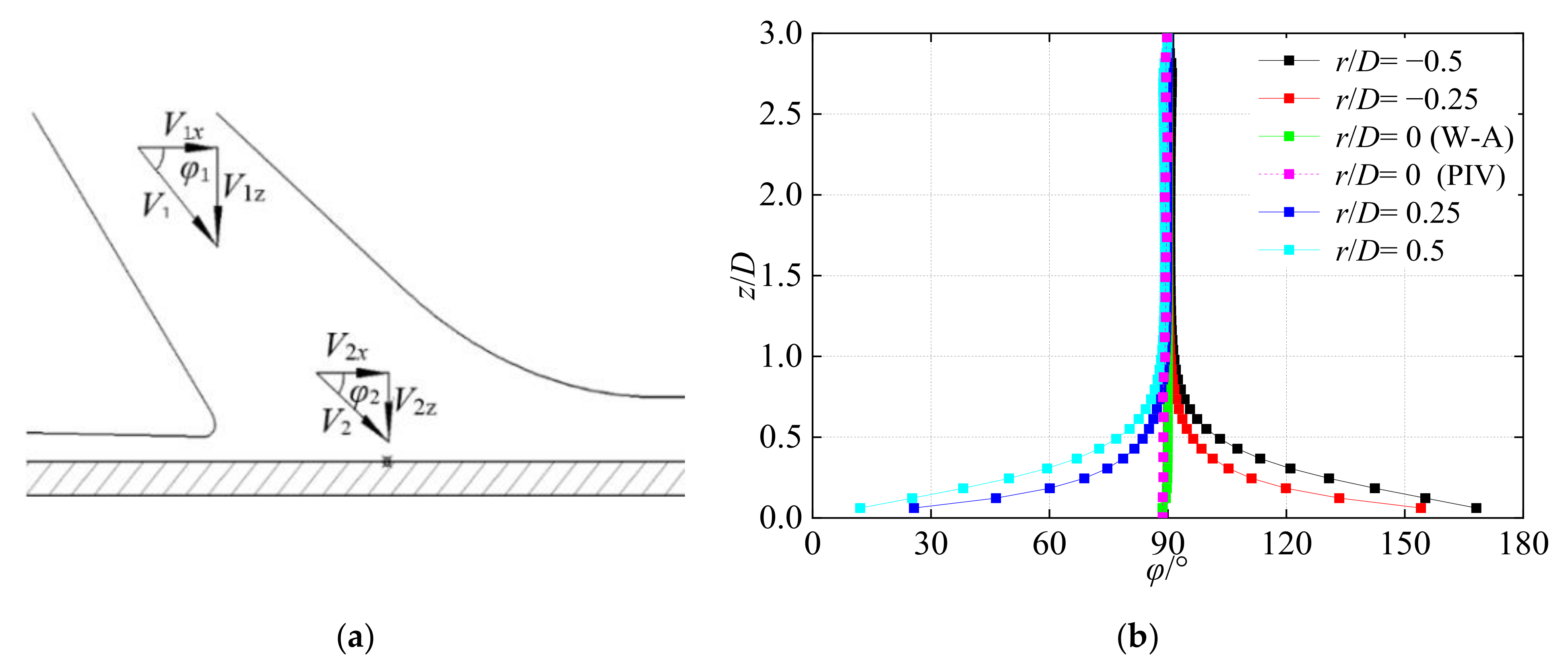
The flow angle φ represents the angle between the flow direction at any point in the cross-section of the flow field and the +x axis, and is given by φ = arctan (−Vz/Vx), as shown in Figure 11a. Figure 11b shows the axial distribution of the flow angle φ at different radial positions in the cross-section of the continuous jet impinging on the stationary wall jet under the condition of impact height H/D = 3 and Reynolds number Re = 35,100. It can be seen from the figure that the flow angle of the jet’s central axis of remains unchanged at 90° and the numerical calculation results are basically consistent with the PIV experimental results. The axial distribution of the flow angles at radial positions symmetrical about the axis of the jet is symmetrical about 90°; at the axial position 1 ≤ z/D ≤ 3, the flow angle φ remains constant at 90°; at the axial position z/D = 1, the jet turns and the flow angle φ starts to change.
3.2. Analysis of the Flow Field of the Impact Jet with Different Impact Heights
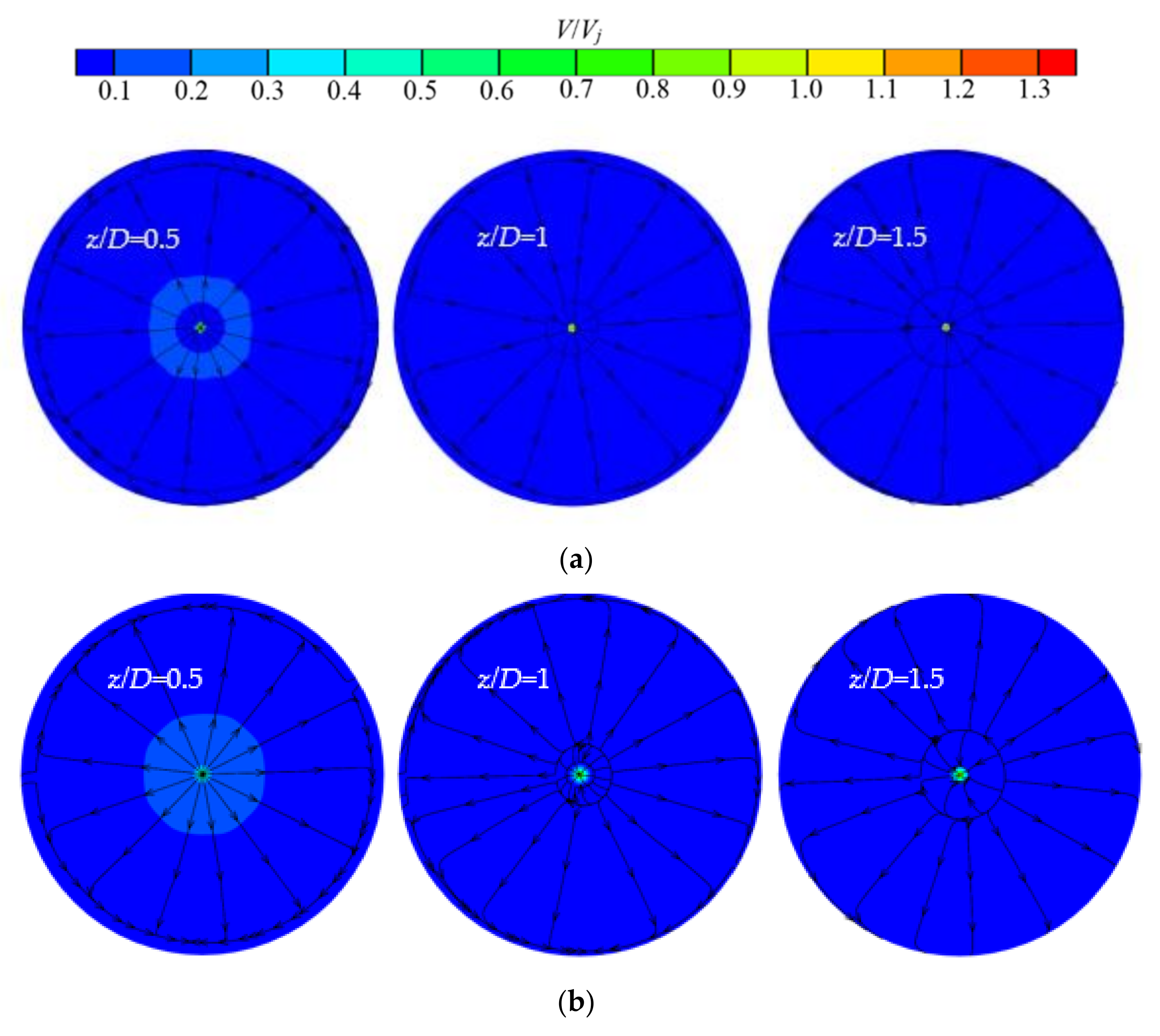
Figure 12 shows the flow structure diagram on the cross-section xoy of the impinging flow field under the conditions of Re = 35,100, H/D = 2 and 8. From the streamline diagram, we can infer that when the cross-sectional height z/D = 0.5, the fluid spreads from the center to the periphery; the flow direction changes and moves in the circumferential direction near the wall of the sink. When the cross-sectional height z/D = 1, the environmental fluid flows toward the edge of the jet due to the jet’s entrainment near the center of the jet. As the cross-sectional height z/D increases, the turning position of the fluid is gradually close to the wall of the tank; the jet velocity increases, the diameter becomes smaller, the coiled suction effect is enhanced, the range of flow to the center of the jet becomes larger, and the range of flow to the surrounding area becomes smaller.
Figure 13 shows the cross-sectional vorticity diagram in the flow field of the continuous jet impacting the stationary wall under the conditions of Reynolds number Re = 35,100 and impact height H/D = 2 and 8. It can be seen from the figure that the vorticity at the center of the jet in the circular pipe is relatively low, and the vorticity near the wall gradually increases; when the jet leaves the pipe, the vorticity distribution area gradually expands with the development of the jet; after reaching the impact wall, the vorticity gradually decreases as the wall jet develops.
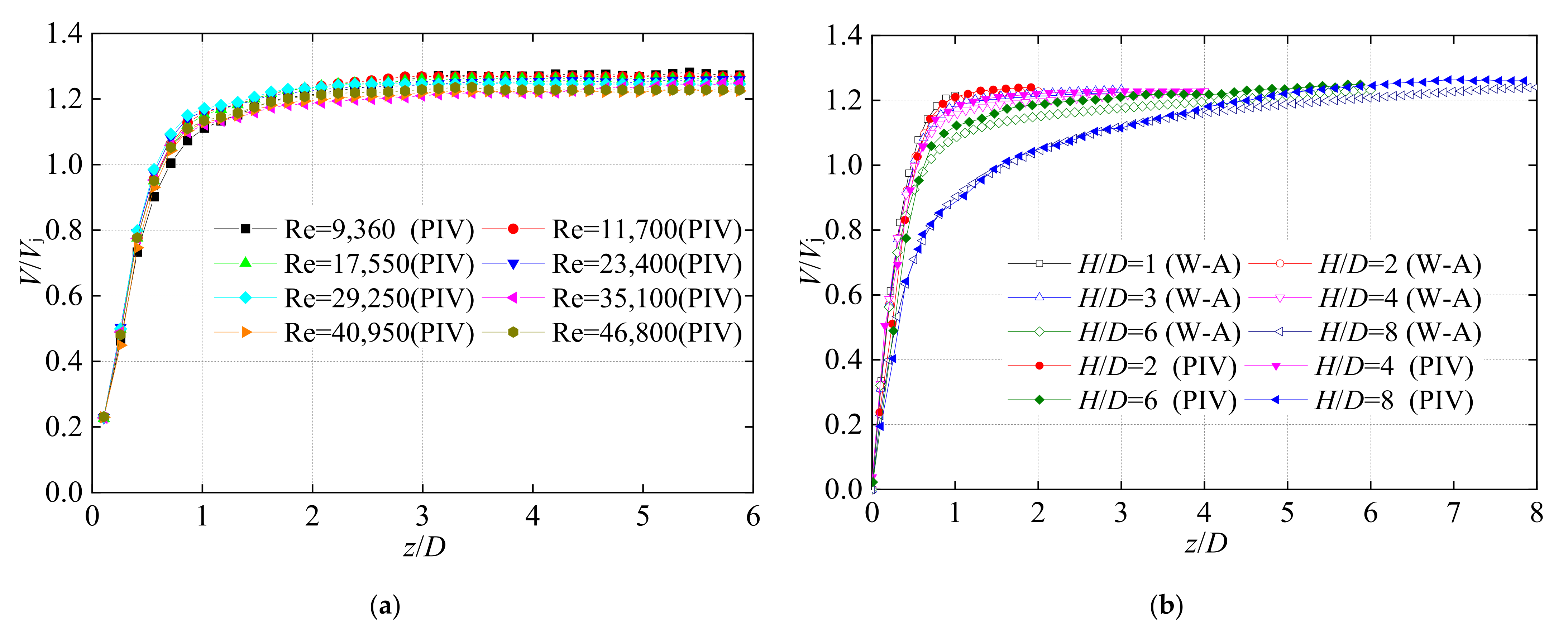
Figure 14a,b show the dimensionless velocity V/Vj distribution on the jet axis under conditions of different Reynolds numbers, with impact height H/D = 6, and different impact heights, with Reynolds number Re = 35,100. It can be seen from Figure 14a that the distribution of the dimensionless velocity V/Vj on the jet axis at different Reynolds numbers almost coincides. This shows that the velocity distribution on the axis is independent of the Reynolds number. It can be seen from Figure 14b that the velocity on the central axis of the jet in the core area remains almost unchanged, and as the impact height increases, the core area gradually increases; the jet velocity decreases rapidly on the centerline of the impact zone, and when it reaches the wall surface, the dimensionless velocity V/Vj decreases to 0, and the height of the impact zone is about 1D. When H/D ≥ 6, the jet has a transition zone, and the jet’s velocity attenuates before reaching the impact zone; as the impact height increases, the transition zone gradually increases, the linear loss gradually increases, and the velocity of the fluid gradually decreases when the fluid reaches the impact zone. After comparing the numerical calculation results with the PIV experiment results at different impact heights, it is found that in the impact zone (0 ≤ z/D ≤ 1), the velocity distribution on the jet center axis is basically the same; in the free-jet zone (z/D ≥ 1), the velocity change trend on the jet center axis is the same, and there is a very small deviation.
3.3. Time-Averaged Pressure Distribution of Impinging Jet
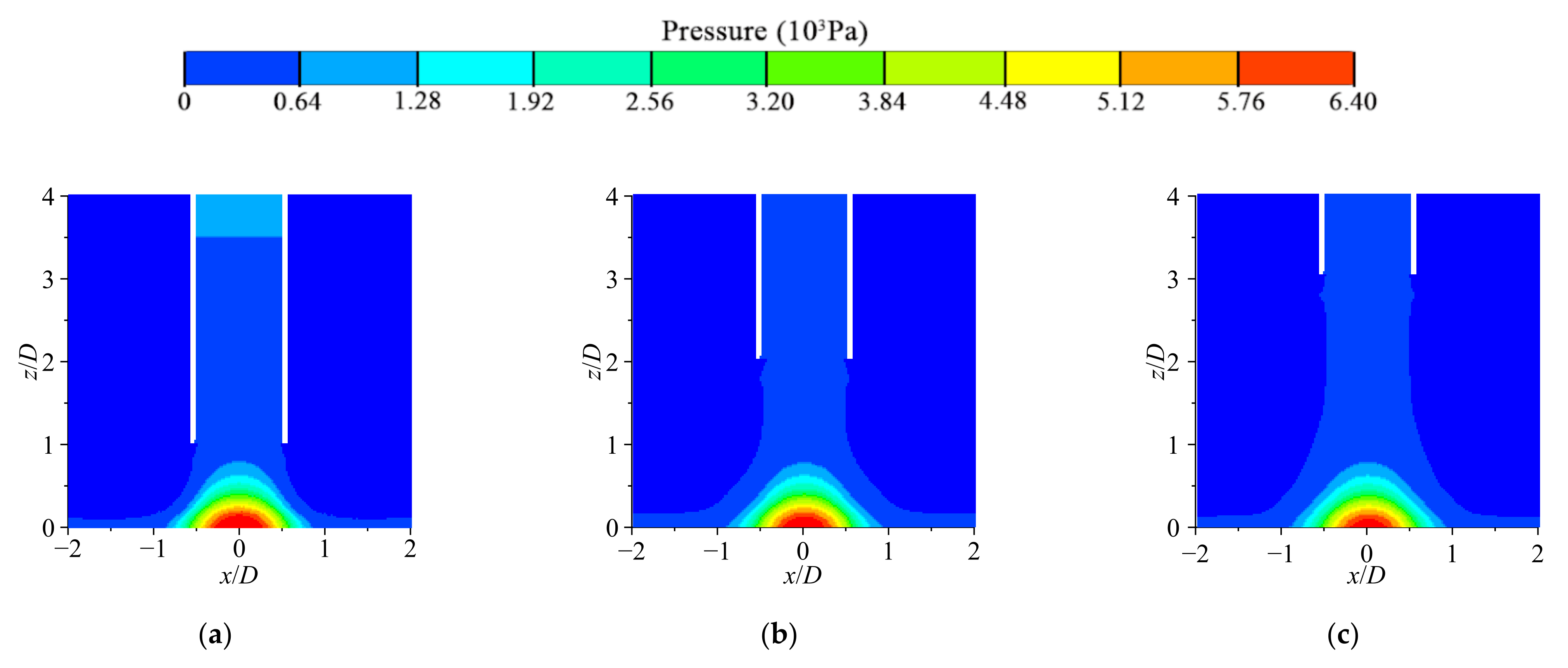
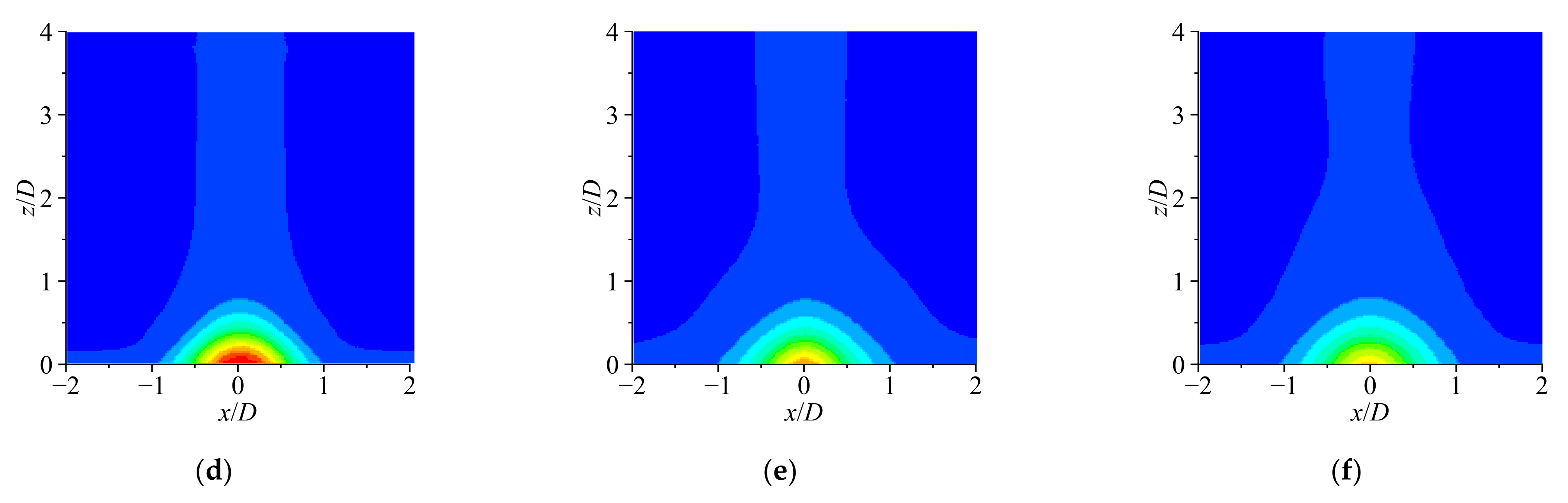
Figure 15 shows the pressure nephogram (Re = 35,100) on the cross-section of the continuous jet impinging on the stationary wall under different impact heights. As can be seen from Figure 15, the pressure in the nozzle gradually decreases with the development of fluid flow; a high-pressure region is formed near the impact origin about the centerline of the jet, symmetrically approximating a semicircle. The pressure is distributed in a semi-annular pattern, and the closer to the impact origin, the higher the pressure. As the impact height increases, the pressure gradually decreases, the size of the high-pressure region is almost constant, and the shape gradually approaches a semicircle.
As a dimensionless number describing the relative pressure in the flow field, the pressure coefficient Cp plays a vital role in the study of fluid mechanics. This paper uses the pressure coefficient Cp to quantitatively analyze the relative pressure in the flow field. The relationship between the pressure coefficient Cp and the dimension is as follows:
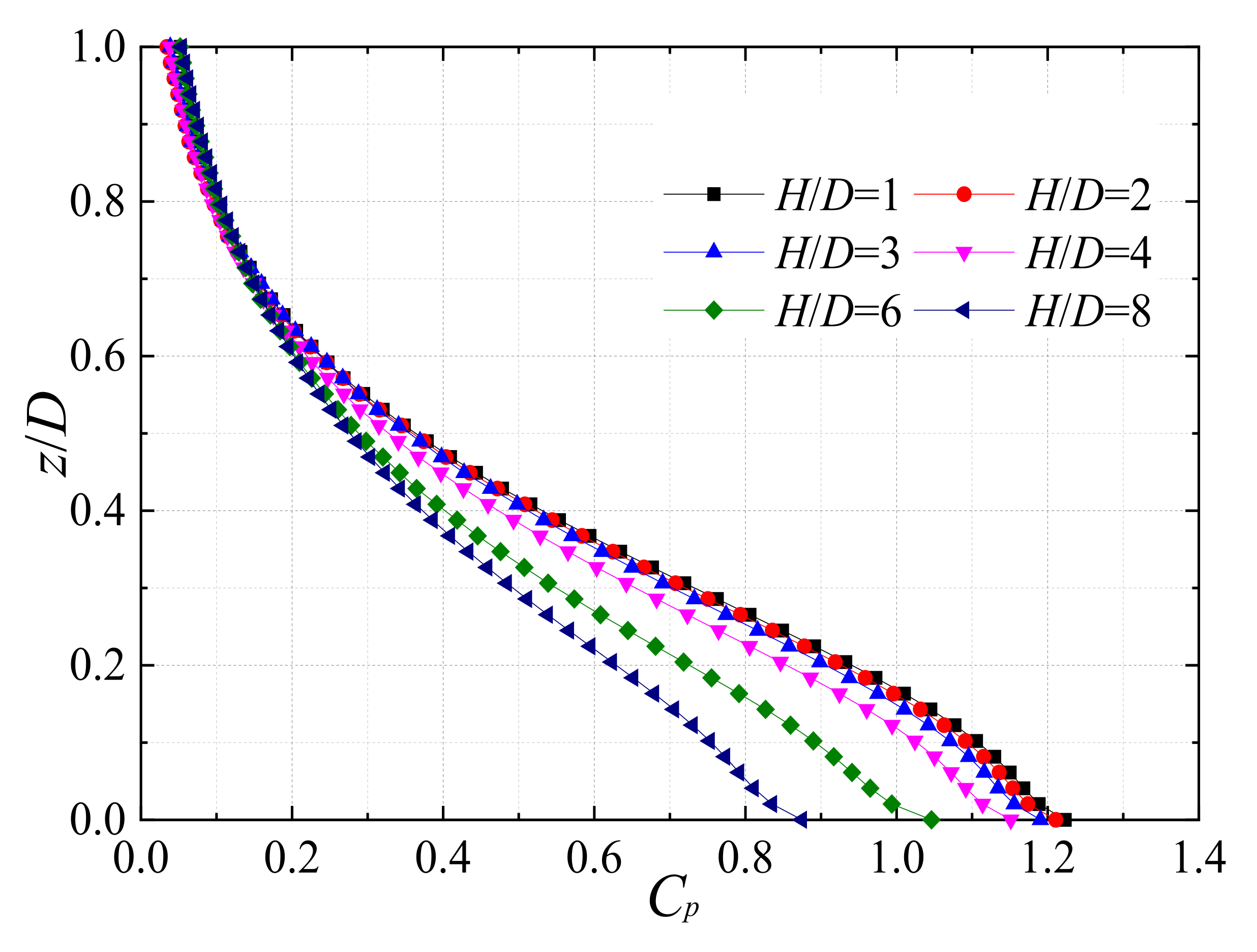
Figure 16 shows the axial distribution of the axial pressure coefficient Cp of the jet at different heights. It can be seen that in the impact zone (0 ≤ z/D ≤ 1), as the axial position z/D decreases, the pressure coefficient Cp gradually increases, and the increasing speed first gradually increases and then gradually decreases. When the axial position 0.65 ≤ z/D ≤ 1, the axial distribution of the axial pressure coefficient Cp of the jet basically coincides under different impact heights; when the axial position 0 ≤ z/D ≤ 0.65, the axial distribution of the axial pressure coefficient Cp of the jet at different impact heights gradually separates as the axial position z/D decreases.
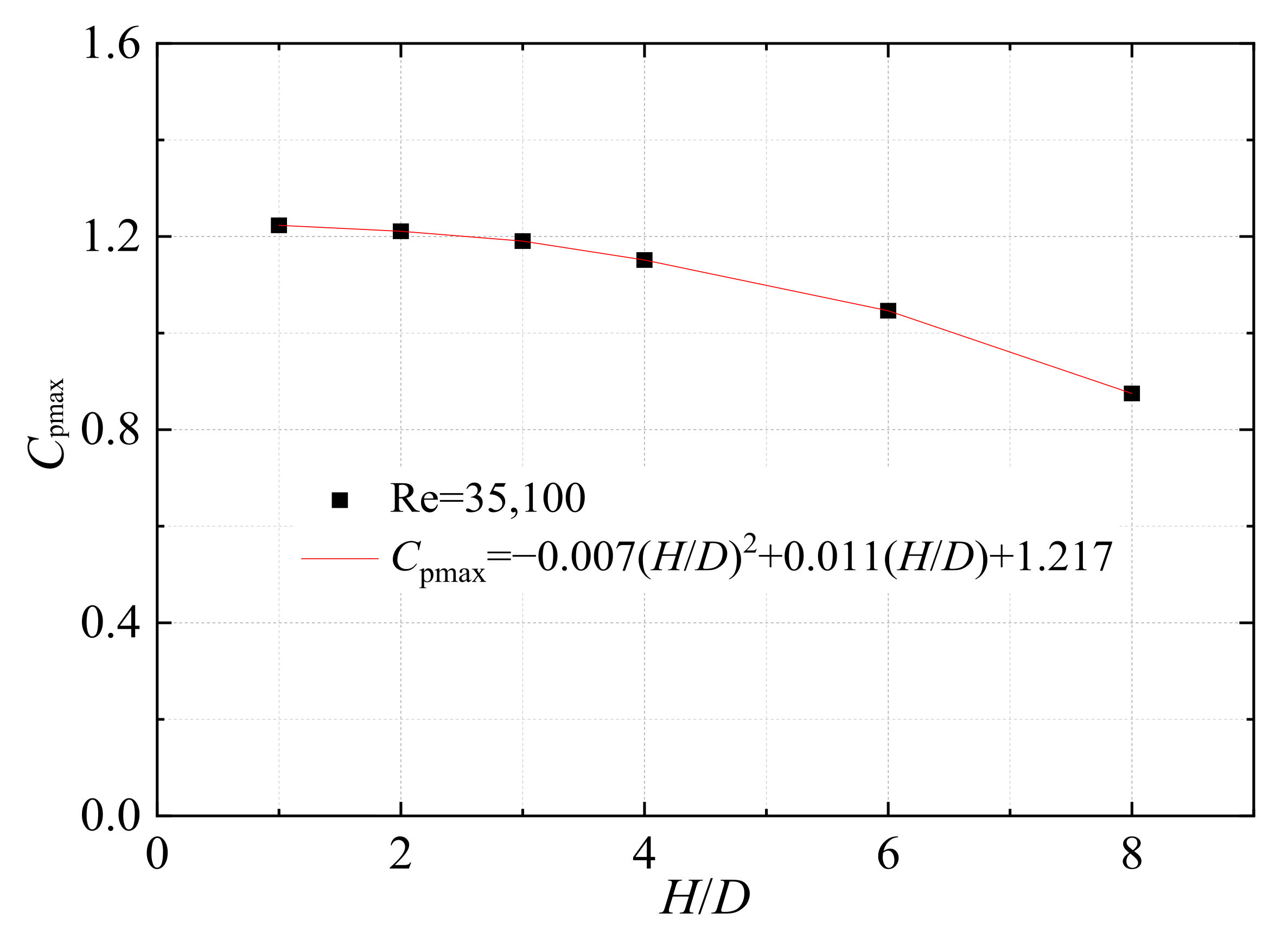
Figure 17 shows the variation in the maximum pressure coefficient Cpmax on the impact wall with the impact height H/D and is fitted with a curve. The fitting formula is
It can be seen from the figure that when the impact height increases from H/D = 2 to H/D = 4, the maximum pressure coefficient decreases from 1.21 to 1.15, which is a decrease of 0.06; when the impact height increases from H/D = 4 to H/D = 6, the maximum pressure coefficient decreases from 1.15 to 1.04, which is a decrease of 0.11; when the impact height increases from H/D = 6 to H/D = 8, the maximum pressure coefficient decreases from 1.04 to 0.87, which is a decrease of 0.17; as the impact height increases, the maximum pressure coefficient Cpmax decreases at a gradually increasing rate.
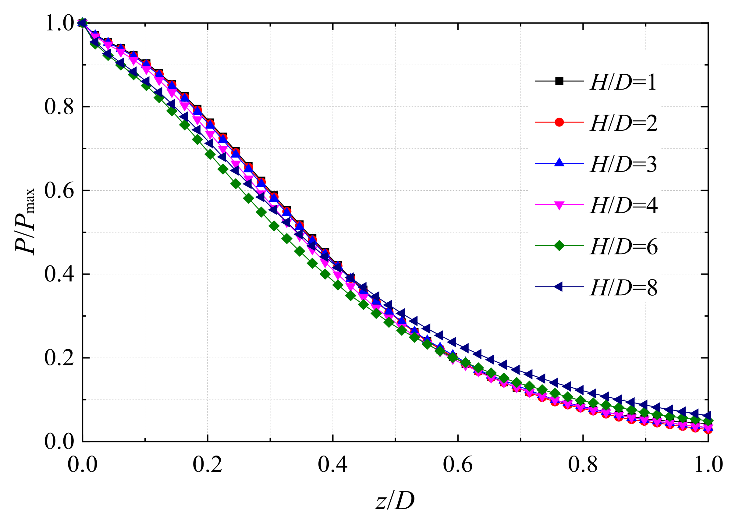
The maximum impact pressure Pmax is used for the dimensionless treatment of the impact pressure. Figure 18 shows the axial distribution of the dimensionless pressure P/Pmax on the axis of the jet at different impact heights. It can be seen from the figure that the axial distribution of the dimensionless pressure P/Pmax on the axis of the jet at different impact heights basically coincides, and the maximum impact pressure is reached at the impact wall. This shows that the pressure distribution on the central axis of the impinging jet at different impact heights has a good similarity. At the same time, we can observe that the figure shows a clear inflection point at z/D = 0.3. The reason is that the fluid is ejected through the nozzle, due to the influence of the surrounding stationary environment fluid, and the axial velocity is rapidly reduced and converted into the pressure energy of the jet as the jet approaches the impact wall; the growth rate of P/Pmax then rises. As the impinging jet gradually approaches the wall, the axial velocity of the jet rapidly becomes zero within a short distance, the kinetic energy contained in the axial velocity of the jet is all converted into pressure energy, P/Pmax reaches its maximum value, and the growth rate of P/Pmax decreases in the near-wall area, resulting in an obvious inflection point in the image at z/D = 0.3.
4. Conclusions
In this paper, continuous submerged impinging jets with different impact heights were investigated using numerical calculations based on the Wray–Agarwal turbulence model. The main conclusions are as follows:
- (1)
- The Wray–Agarwal turbulence model is able to better predict the flow characteristics when a continuous jet impinges on a stationary wall. It is found through numerical simulations that the jet flow structure depends on impact height H/D and is relatively independent of the Reynolds number.
- (2)
- The dimensionless average velocity V/Vj along the centerline of the jet remains constant in the core region but drops rapidly in the transition and impact region. As the impact height increases, the degree of diffusion of the jet reaching the impact region increases, and the velocity gradually decreases. Near the stagnation point (x/D = 0), the fluid radial velocity first increases and then decreases.
- (3)
- The pressure coefficient Cp on the jet axis increases gradually with the decrease in the axial position z/D, and the increasing trend first increases and then decreases. As the impact height increases, the maximum pressure coefficient Cpmax gradually decreases, and the rate of decrease gradually increases.
- (4)
- The dimensionless pressure P/Pmax distribution basically coincides under different impact heights, and all reach the maximum impact pressure at the impact wall.
The above conclusions can provide some theoretical guidance to marine engineering. In the case of underwater dredging, reef cutting, or hull cleaning, the impact distance can be controlled to achieve different engineering effects under a certain amount of water injection. At the same time, we should also pay attention to the diffusion area formed after the jet impacts the wall in actual marine engineering. We believe that the diffusion area can effectively remove the waste materials generated by underwater dredging and other projects, an idea that needs to be further studied. In addition, the pressure law at the impact point of the jet should also be considered, and we should make good use of the impact point of the jet to achieve the best engineering application.
Author Contributions
Data curation, H.W. and Y.Z. (Yong Zhu); formal analysis, B.H. and J.L.; writing—original draft preparation, B.H. and Y.Z. (Yingchong Zhang); writing—review and editing, C.W. and J.G. All authors have read and agreed to the published version of the manuscript.
Funding
This research was supported by the National Key R&D Program of China (Grant No: 2020YFC1512402), Open Research Fund of State Key Laboratory of Simulation and Regulation of Water Cycle in River Basin (China Institute of Water Resources and Hydropower Research), Grant No: IWHR-SKL-201719, the National Natural Science Foundation of China (Grant No: 51979240 and 51609105).
Institutional Review Board Statement
Not applicable.
Informed Consent Statement
Not applicable.
Data Availability Statement
Not applicable.
Conflicts of Interest
The authors declare no conflict of interest.
References
- Dong, Z. Impinging Jets; China Ocean Press: Beijing, China, 1997. [Google Scholar]
- Wang, L.; Wang, G. Experimental and Theoretical Study on the Critical Breaking Velocity of Marine Natural Gas Hydrate Sediments Breaking by Water Jet. Energies 2020, 13, 1725. [Google Scholar] [CrossRef] [Green Version]
- Liu, G.; Yuan, Z.; Incecik, A.; Leng, D.; Wang, S.; Li, Z. A new biomimetic antifouling method based on water jet for marine structures. Proc. Inst. Mech. Eng. Part M J. Eng. Marit. Environ. 2020, 234, 573–584. [Google Scholar] [CrossRef]
- Song, C.; Cui, W. Review of underwater ship hull cleaning technologies. J. Mar. Sci. Appl. 2020, 19, 415–429. [Google Scholar] [CrossRef]
- Atangana Njock, P.G.; Zheng, Q.; Zhang, N.; Xu, Y.S. Perspective Review on Subsea Jet Trenching Technology and Modeling. J. Mar. Sci. Eng. 2020, 8, 460. [Google Scholar] [CrossRef]
- Liu, G.; Jiang, W.; Yuan, Z.; Xie, Y.; Tian, X.; Leng, D.; Atilla, I.; Li, Z. Design and optimization of a water jet-based biomimetic antifouling model for marine structures. Phys. Fluids 2020, 32, 097101. [Google Scholar] [CrossRef]
- Fitzgerald, J.A.; Garimella, S.V. A study of the flow field of a confined and submerged impinging jet. Int. J. Heat Mass Transf. 1998, 41, 1025–1034. [Google Scholar] [CrossRef]
- Abdel-Fattah, A. Numerical and experimental study of turbulent impinging twin-jet flow. Exp. Therm. Fluid Sci. 2007, 31, 1061–1072. [Google Scholar] [CrossRef]
- Hassan, M.E.; Assoum, H.H.; Sobolik, V.; Abed-Meraim, K.; Sakout, A. Experimental investigation of the wall shear stress in a circular impinging jet. Phys. Fluids 2013, 25, 106–115. [Google Scholar] [CrossRef]
- Charmiyan, M.; Azimian, A.R.; Shirani, E.; Aloui, F.; Degouet, C.; Michaelis, D. 3D tomographic PIV, POD and vortex identification of turbulent slot jet flow impinging on a flat plate. J. Mech. Sci. Technol. 2017, 31, 5347–5357. [Google Scholar] [CrossRef]
- Pieris, S.; Zhang, X.; Yarusevych, S.; Peterson, S.D. Evolution of coherent structures in a two-dimensional impinging jet. In Tenth International Symposium on Turbulence and Shear Flow Phenomena; Tsfp Digital Library Online; Begel House Inc.: Danbury, CT, USA, 2017. [Google Scholar]
- Markal, B.; Aydin, O. Experimental Investigation of Coaxial Impinging Air Jets. Appl. Therm. Eng. 2018, 141, 1120–1130. [Google Scholar] [CrossRef]
- Zhang, L.; Wang, C.; Zhang, Y.; Xiang, W.; He, Z.; Shi, W. Numerical study of coupled flow in blocking pulsed jet impinging on a rotating wall. J. Braz. Soc. Mech. Sci. Eng. 2021, 43, 508. [Google Scholar] [CrossRef]
- Xu, K.; Zhang, P. Numerical prediction of turbulent heat transfer in a semi-confined impinging jet. J. Trans. Beijing Inst. Technol. 2003, 23, 540–544. [Google Scholar]
- Chen, Q.; Xu, Z.; Zhang, Y. Numerical Simulation of Turbulent Impinging Jet Flow Using a Modified Renormalization Group Model. J. Xian Jiaotong Univ. 2002, 36, 916–920. [Google Scholar]
- Jiao, L.; Wang, L.; Xu, R.; Li, J. Numerical Predicting of The Effect of Jet-To-Target Plate Spacing on Submerged Impinging Jet Flow. J. Eng. Thermophys. 2005, 26, 773–775. [Google Scholar]
- Bhatti, M.M.; Alamri, S.Z.; Ellahi, R.; Abdelsalam, S.I. Intra-uterine particle–fluid motion through a compliant asymmetric tapered channel with heat transfer. J. Therm. Anal. Calorim. 2021, 144, 2259–2267. [Google Scholar] [CrossRef]
- Bhatti, M.M.; Abdelsalam, S.I. Thermodynamic entropy of a magnetized Ree-Eyring particle-fluid motion with irreversibility process: A mathematical paradigm. ZAMM J. Appl. Math. Mech. 2020, 101, e202000186. [Google Scholar] [CrossRef]
- Abumandour, R.M.; Eldesoky, I.M.; Kamel, M.H.; Ahmed, M.M.; Abdelsalam, S.I. Peristaltic thrusting of a thermal-viscosity nanofluid through a resilient vertical pipe. Z. Nat. A 2020, 75, 727–738. [Google Scholar] [CrossRef]
- Abdelsalam, S.I.; Zaher, A.Z. Leveraging elasticity to uncover the role of rabinowitsch suspension through a wavelike conduit: Consolidated blood suspension application. Mathematics 2021, 9, 2008. [Google Scholar] [CrossRef]
- Raza, R.; Mabood, F.; Naz, R.; Abdelsalam, S.I. Thermal transport of radiative Williamson fluid over stretchable curved surface. J. Therm. Sci. Eng. Prog. 2021, 23, 100887. [Google Scholar] [CrossRef]
- Bhatti, M.M.; Abdelsalam, S.I. Bio-inspired peristaltic propulsion of hybrid nanofluid flow with Tantalum (Ta) and Gold (Au) nanoparticles under magnetic effects. Waves Random Complex Media 2021, 1–26. [Google Scholar] [CrossRef]
- Huo, W.; Li, Z.; Wang, J.; Yao, C.; Zhang, K.; Huang, Y. Multiple hydrological models comparison and an improved Bayesian model averaging approach for ensemble prediction over semi-humid regions. Stoch. Environ. Res. Risk Assess. 2019, 33, 217–238. [Google Scholar] [CrossRef]
- Zhang, Z.; Luo, C.; Zhao, Z. Application of probabilistic method in maximum tsunami height prediction considering stochastic seabed topography. Nat. Hazards 2020, 104, 2511–2530. [Google Scholar] [CrossRef]
- Xu, J.; Lan, W.; Ren, C.; Zhou, X.; Wang, S.; Yuan, J. Modeling of coupled transfer of water, heat and solute in saline loess considering sodium sulfate crystallization. J. Cold Reg. Sci. Technol. 2021, 189, 103335. [Google Scholar] [CrossRef]
- Zhang, Y.; Zhang, F.; Xu, Y.; Huang, W.; Wu, L.; Dong, Z.; Zhang, Y.; Dong, B.; Zhang, X.; Zhang, H. Epitaxial Growth of Topological Insulators on Semiconductors (Bi2Se3/Te@ Se) toward High-Performance Photodetectors. Small Methods 2019, 3, 1900349. [Google Scholar] [CrossRef]
- Wang, J.; Ai, K.; Lu, L. Flame-retardant porous hexagonal boron nitride for safe and effective radioactive iodine capture. J. Mater. Chem. A. 2019, 7, 16850–16858. [Google Scholar] [CrossRef]
- Wang, X.; Lyu, X. Experimental study on vertical water entry of twin spheres side-by-side. Ocean Eng. 2021, 221, 108508. [Google Scholar] [CrossRef]
- Wu, H.; Zhang, F.; Zhang, Z. Droplet breakup and coalescence of an internal-mixing twin-fluid spray. Phys. Fluids 2021, 33, 013317. [Google Scholar] [CrossRef]
- Bhatti, M.M.; Marin, M.I.; Zeeshan, A.; Abdelsalam, S.I. Recent trends in computational fluid dynamics. Front. Phys. 2020, 8, 453. [Google Scholar] [CrossRef]
- Zhu, Y.; Li, G.; Wang, R.; Tang, S.; Su, H.; Cao, K. Intelligent fault diagnosis of hydraulic piston pump combining improved lenet-5 and pso hyperparameter optimization. Appl. Acoust. 2021, 183, 108336. [Google Scholar] [CrossRef]
- Shi, L.; Zhu, J.; Tang, F.; Wang, C. Multi-Disciplinary optimization design of axial-flow pump impellers based on the approximation model. Energies 2020, 13, 779. [Google Scholar] [CrossRef] [Green Version]
- Zhou, J.; Zhao, M.; Wang, C.; Gao, Z. Optimal design of diversion piers of lateral intake pumping station based on orthogonal test. Shock. Vib. 2021, 5, 1–9. [Google Scholar] [CrossRef]
- Wang, H.; Hu, Q.; Yang, Y.; Wang, C. Performance differences of electrical submersible pump under variable speed schemes. Int. J. Simul. Model. 2021, 20, 76–86. [Google Scholar] [CrossRef]
- Lin, Y.; Li, X.; Li, B.; Jia, X.; Zhu, Z. Influence of impeller sinusoidal tubercle trailing edge on pressure pulsation in a centrifugal pump at nominal flow rate. ASME J. Fluids Eng. 2021, 143, 091205. [Google Scholar] [CrossRef]
- Lin, T.; Zhu, Z.; Li, X.; Li, J.; Lin, Y. Theoretical, experimental, and numerical methods to predict the best efficiency point of centrifugal pump as turbine. Renew. Energy 2021, 168, 31–44. [Google Scholar] [CrossRef]
- Khan, A.; Irfan, M.; Niazi, U.M.; Shah, I.; Legutko, S.; Rahman, S.; Alwadie, A.S.; Jalalah, M.; Glowacz, A.; Khan, M.K.A. Centrifugal Compressor Stall Control by the Application of Engineered Surface Roughness on Diffuser Shroud Using Numerical Simulations. Materials 2021, 14, 2033. [Google Scholar] [CrossRef] [PubMed]
- Yang, Y.; Zhou, L.; Hang, J.; Du, D.; Shi, W.; He, Z. Energy characteristics and optimal design of diffuser meridian in an electrical submersible pump. Renew. Energy 2021, 167, 718–727. [Google Scholar] [CrossRef]
- Wang, H.; Long, B.; Wang, C.; Han, C.; Li, L. Effects of the impeller blade with a slot structure on the centrifugal pump performance. Energies 2020, 13, 1628. [Google Scholar] [CrossRef]
- Li, X.; Shen, T.; Li, P.; Guo, X.; Zhu, Z. Extended compressible thermal cavitation model for the numerical simulation of cryogenic cavitating flow. Int. J. Hydrog. Energy 2020, 45, 10104–10118. [Google Scholar] [CrossRef]
- Yang, Y.; Zhou, L.; Shi, W.; He, Z.; Han, Y.; Xiao, Y. Interstage difference of pressure pulsation in a three-stage electrical submersible pump. J. Pet. Sci. Eng. 2021, 196, 107653. [Google Scholar] [CrossRef]
- Yang, Y.; Zhou, L.; Bai, L.; Xu, H.; Lv, W.; Shi, W.; Wang, H. Numerical Investigation of Tip Clearance Effects On the Performance and Flow Pattern within a Sewage Pump. J. Fluids Eng. 2022, FE-21-1345. [Google Scholar] [CrossRef]
- Zhang, X.; Agarwal, R.K.; Gao, H.; Zhou, L. Numerical Investigation of a Submerged Water Jet Impinging at Various Angles on Ground. In Proceedings of the AIAA Scitech 2020 Forum, Orlando, FL, USA, 6–10 January 2020; p. 2038. [Google Scholar]
- Han, Y.; Zhou, L.; Bai, L.; Shi, W.; Agarwal, R. Comparison and validation of various turbulence models for U-bend flow with a magnetic resonance velocimetry experiment. Phys. Fluids 2021, 33, 125117. [Google Scholar] [CrossRef]
- Cooper, D.; Jackson, D.C.; Launder, B.E.; Liao, G.X. Impinging jet studies for turjulence model assessment—I. Flow-field experiments. Int. J. Heat Mass Transf. 1993, 36, 2675–2684. [Google Scholar] [CrossRef]
Figure 1.
Schematic diagram of jet impacting a stationary disk.

Figure 2.
The average velocity of the cross-section in the jet.

Figure 3.
Grid of submerged impinging jet calculation model.

Figure 4.
The axial distribution of the dimensionless velocity V/Vj at the center of the jet.

Figure 5.
Dimensionless velocity V/Vj distribution nephogram in the cross-section of a circular pipe.
Figure 5.
Dimensionless velocity V/Vj distribution nephogram in the cross-section of a circular pipe.

Figure 6.
The radial distribution of the dimensionless velocity V/Vj at different tube positions.

Figure 7.
Radial distribution of dimensionless velocity V/Vmax under different Reynolds numbers.

Figure 8.
The flow structure of a continuous jet impacting a stationary wall: (a) full flow field; (b) cross-section of flow field; (c) near wall.
Figure 8.
The flow structure of a continuous jet impacting a stationary wall: (a) full flow field; (b) cross-section of flow field; (c) near wall.

Figure 9.
The radial distribution of the dimensionless velocity V/Vj at different axial positions in the cross-section of the jet: (a) Re = 11,700; (b) Re = 23,400; (c) Re = 35,100.
Figure 9.
The radial distribution of the dimensionless velocity V/Vj at different axial positions in the cross-section of the jet: (a) Re = 11,700; (b) Re = 23,400; (c) Re = 35,100.

Figure 10.
Axial distribution of velocity V/Vj at different radial positions of the cross-section in the jet.
Figure 10.
Axial distribution of velocity V/Vj at different radial positions of the cross-section in the jet.

Figure 11.
(a) Schematic diagram of the flow angle φ; (b) the axial distribution of the flow angle φ at different radial positions in the cross-section of the jet.
Figure 11.
(a) Schematic diagram of the flow angle φ; (b) the axial distribution of the flow angle φ at different radial positions in the cross-section of the jet.

Figure 12.
Flow structure diagram of different cross-sections of continuous jet impinging on stationary wall: (a) H/D = 2; (b) H/D = 8.
Figure 12.
Flow structure diagram of different cross-sections of continuous jet impinging on stationary wall: (a) H/D = 2; (b) H/D = 8.

Figure 13.
Cross-sectional vorticity diagram in the flow field at different H/D: (a) H/D = 2; (b) H/D = 8.
Figure 13.
Cross-sectional vorticity diagram in the flow field at different H/D: (a) H/D = 2; (b) H/D = 8.

Figure 14.
Distribution of dimensionless velocity V/Vj on the axis of the jet: (a) different Reynolds numbers; (b) different impact heights.
Figure 14.
Distribution of dimensionless velocity V/Vj on the axis of the jet: (a) different Reynolds numbers; (b) different impact heights.

Figure 15.
Nephogram of cross-sectional pressure distribution in impinging jets at different impact heights: (a) H/D = 1; (b) H/D = 2; (c) H/D = 3; (d) H/D = 4; (e) H/D = 6; (f) H/D = 8.
Figure 15.
Nephogram of cross-sectional pressure distribution in impinging jets at different impact heights: (a) H/D = 1; (b) H/D = 2; (c) H/D = 3; (d) H/D = 4; (e) H/D = 6; (f) H/D = 8.


Figure 16.
Distribution of the axial pressure coefficient Cp of the jet in the impingement zone.

Figure 17.
Change in maximum pressure coefficient Cpmax on the impact wall at different impact heights H/D.
Figure 17.
Change in maximum pressure coefficient Cpmax on the impact wall at different impact heights H/D.

Figure 18.
The axial distribution of dimensionless pressure P/Pmax on the axis of the jet in the impingement region.
Figure 18.
The axial distribution of dimensionless pressure P/Pmax on the axis of the jet in the impingement region.


Table 1.
The advantages and improvements of this paper, compared with existing literature.
| Existing Literature | Turbulence Model Used | The Improvements of This Paper Compared with the Literature |
|---|---|---|
| Xu et al. [14] | Standard k–ε RNG k–ε with wall function Low Reynolds number k–ε | In the literature, all three turbulence models failed to predict the flow characteristics and heat transfer properties of the impinging jet field completely and accurately, but the Wray–Agarwal turbulence model used in this paper agrees well with the experimental data and predicts the flow structure of the impinging jet more accurately. |
| Chen et al. [15] | Improved RNG k–ε | The accuracy of the improved RNG k–ε turbulence model used in the literature has been improved somewhat, but there are still some errors in the prediction of the mean velocity and turbulent kinetic energy in the near-wall region. However, compared with the Particle Image Velocimetry (PIV) experimental results, the Wray–Agarwal turbulence model used in this paper solves the prediction problem of the flow in the near-wall region better and the error is better controlled. |
| Jiao et al. [16] | Standard k–ε | The literature and the previous two have reached similar conclusions that the standard model cannot accurately predict the flow structure and turbulence intensity distribution in the impact zone and near-wall flow of a water jet impinging on a flat plate. With reference to the high-precision PIV experimental data, the numerical simulation results in this paper have strongly demonstrated that the Wray–Agarwal turbulence model has good results in simulating the flow in the near-wall region of the impinging jet. |
Publisher’s Note: MDPI stays neutral with regard to jurisdictional claims in published maps and institutional affiliations. |
© 2022 by the authors. Licensee MDPI, Basel, Switzerland. This article is an open access article distributed under the terms and conditions of the Creative Commons Attribution (CC BY) license (https://creativecommons.org/licenses/by/4.0/).
Share and Cite
MDPI and ACS Style
Hu, B.; Wang, H.; Liu, J.; Zhu, Y.; Wang, C.; Ge, J.; Zhang, Y. A Numerical Study of a Submerged Water Jet Impinging on a Stationary Wall. J. Mar. Sci. Eng. 2022, 10, 228. https://0-doi-org.brum.beds.ac.uk/10.3390/jmse10020228
AMA Style
Hu B, Wang H, Liu J, Zhu Y, Wang C, Ge J, Zhang Y. A Numerical Study of a Submerged Water Jet Impinging on a Stationary Wall. Journal of Marine Science and Engineering. 2022; 10(2):228. https://0-doi-org.brum.beds.ac.uk/10.3390/jmse10020228
Chicago/Turabian StyleHu, Bo, Hui Wang, Jinhua Liu, Yong Zhu, Chuan Wang, Jie Ge, and Yingchong Zhang. 2022. "A Numerical Study of a Submerged Water Jet Impinging on a Stationary Wall" Journal of Marine Science and Engineering 10, no. 2: 228. https://0-doi-org.brum.beds.ac.uk/10.3390/jmse10020228
Note that from the first issue of 2016, this journal uses article numbers instead of page numbers. See further details here.