Sliding Mode Motion Control for AUV with Dual-Observer Considering Thruster Uncertainty

Abstract

In the motion control of AUVs, especially those driven by multiple thrusters, the thruster misalignment and thrust loss cause the actual force and moment applied to the AUV to deviate from that desired, making accurate and fast motion control difficult. This paper proposes a sliding mode control method with dual-observer estimation for the AUV 3D motion control problem in the presence of thruster misalignment uncertainty and thrust loss uncertainty. Firstly, this paper considers the force and moment deviation as disturbances that vary with the controller output, and proposes the TD disturbance observer to address the problem of deviation caused by uncertainty in thruster misalignment. Secondly, this paper introduces the dynamics equation of thrust loss and designs the gain disturbance observer to estimate the thrust loss uncertainty during AUV navigation. The designed controller, verified by simulation and field tests, ensures that the AUV maintains better motion control despite thruster misalignment and thrust loss.

1. Introduction

AUV has been an active field of research and development in exploring unknown marine environments and carrying out different military missions [1]. One of the critical bottlenecks in developing AUVs is the technology readiness level (TRL) in the motion control area. Motion control algorithm design for AUVs is a hard task for the following reasons: the finite force and moment, velocity and acceleration, inherent nonlinear dynamics, structural and nonstructural uncertainties, external disturbances, time-varying parameters, time-varying environment, shallow water effect, coupling between degrees of freedom (DOFs), and the limited number of actuators with respect to the DOFs (under actuator constraints) [2]. Therefore, it is important to consider the above reasons when developing motion control algorithms for AUVs. In the actual operating environment of an AUV, there will inevitably be uncertain misalignment in thrusters due to manufacturing tolerances. Small misalignment has no significant impact on control performance. However, for attitude tracking, especially for fast-tracking of multi-thruster-driven AUV, thruster misalignment will cause significant attitude tracking errors [3]. Moreover, the presence of influences such as incoming flow velocity and thruster motor friction will all cause uncertain thrust losses from the thruster, which will not achieve the desired thrust and will affect the dynamic performance of the vehicle [4]. These problems of AUV control force and moment deviation caused by thruster uncertainty cannot be ignored in the design of the controller. Some research ideas have been proposed on controller design studies to cope with the actuator uncertainty problem. Yoon H [5] proposed an adaptive control algorithm for attitude tracking in the case of uncertainty in actuator misalignment. The proposed adaptive law applies a smooth projection algorithm to keep the parameter estimation in the singular-free region, but had the defect of having too many estimated parameters. Qinglei Hu [6] proposed an adaptive control law to solve the moment deviation caused by actuator misalignment. Xiao B [7] proposed a VSC-based compensation scheme for actuator misalignment and faults, which drove attitude tracking errors and velocity tracking errors to zero in a limited time. Zhang J [8] designed a new ESO based on SOSM technology and added a linear correction term to estimate the disturbance caused by actuator misalignment in a finite time, and then proposed an adaptive fast terminal sliding mode controller. Zhang F [9] proposed a backstepping control method based on adaptive filtering for 6-DOF translation and attitude tracking control with actuator misalignment. All the above studies solved the problem of the uncertainty of installation deviation from the control level of the actuator or solved the control law of the carrier by solving the pseudo inverse of the control law of the actuator. In some studies, the method of disturbance observer is proposed for observation compensation, which provides research ideas for this paper.

Different research approaches have been proposed by some scholars to address the uncertainty of thrust loss. Dydek Z [10] designed an augmented adaptive controller to reduce the impact of abnormal thrust loss while considering the impact of dead zones. Cao L et al. [11] estimated the uncertainty of the actuator based on the observer, and designed a nonsingular terminal sliding mode controller by using this estimation and full-state measurement. Cao L et al. [12] proposed an observer-based exponential elastic control method to achieve fast and highly accurate attitude tracking maneuvers. The thrust loss problem in the above studies is mainly the uncertainty caused by thruster damage or failure, which is different from the thrust loss caused by AUV navigation studied in this paper. Luca P [13] proposed a thruster thrust estimation scheme consisting of a nonlinear thruster moment observer and a mapping of thrust generated from the observed moment, with the forward speed assumed to be unknown and obtained in experimental tests’ accurate results. TI Fossen [14] used three kinds of state models of thruster speed, carrier forward velocity, and axial velocity to reconstruct axial velocity, and designed a nonlinear observer of thruster axial velocity to estimate thrust and moment loss. Kim S Y [15] proposed a thrust loss suppression algorithm, which regarded the thrust loss caused by thruster cavitation as the disturbance moment. The disturbance moment is estimated by a disturbance observer. The thruster speed reference is corrected to suppress the thrust loss by considering the disturbance moment. Cecchi D [16] considered the quasi-static equations of motion, deduced the relationship between forwarding velocity and thruster speed, realized the identification of the quasi-static thrust model of AUV, and designed a simple speed controller. Zhang L [17] proposed an anti-windup intelligent integral method based on the S-surface control idea, which determined the adaptive weight by estimating the motion state of the underwater vehicle and processed the constantly changing propulsion loss. Finally, speed control, yaw control, and depth control experiments were carried out. The above studies put forward different solutions to the problem of thrust loss generated during navigation, but they are all aimed at the carrier with joint rudder-thruster control, which is different from the multi-thruster-driven carrier studied in this paper. The rest of this paper is organized as follows. In the second part, this paper establishes the kinematics and dynamics equations of AUV and establishes the thruster misalignment model and the thrust loss model. Then, this paper analyzes the influence of the two uncertainties on the control. In the third part, the observer is designed based on the tracking differentiator to estimate the disturbance force and moment in the presence of thruster misalignment, and the stability of the TD observer is also demonstrated. Considering the uncertainty of thrust loss, this paper designs a gain disturbance observer to estimate thrust loss, and then proves the stability of the gain observer. In the fourth part, the simulation experiment is carried out, which proves the effectiveness of the two disturbance observers and ensures the motion control effect in the presence of thruster misalignment and thrust loss. In the fifth part, a field test is carried out, which verifies the effectiveness of the controller.

The main contributions of this paper are as follows:

• Firstly, this paper proposes a disturbance observer based on a tracking differentiator for AUV motion control with the uncertainty of thruster misalignment. The force and moment deviations are regarded as disturbances with the change of control force. A three-dimensional sliding mode motion controller is proposed based on the disturbance observer, and the stability of the controller and convergence of the TD disturbance observer is proved theoretically.
• Secondly, this paper introduces the thruster dynamics model and proposes the gain disturbance observer to estimate the uncertainty of thruster thrust loss. Then, it theoretically proves the convergence of the gain disturbance observer.

2. Problem Statement

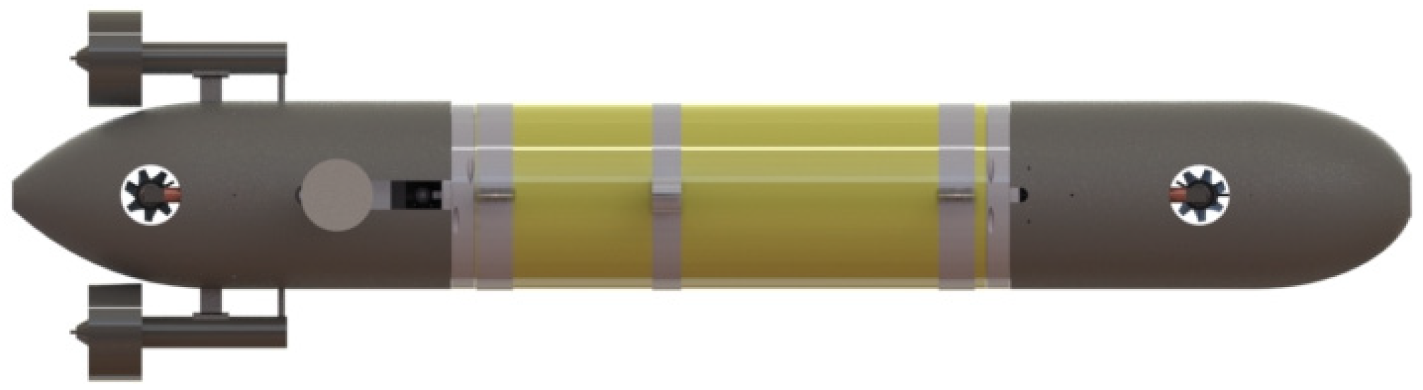
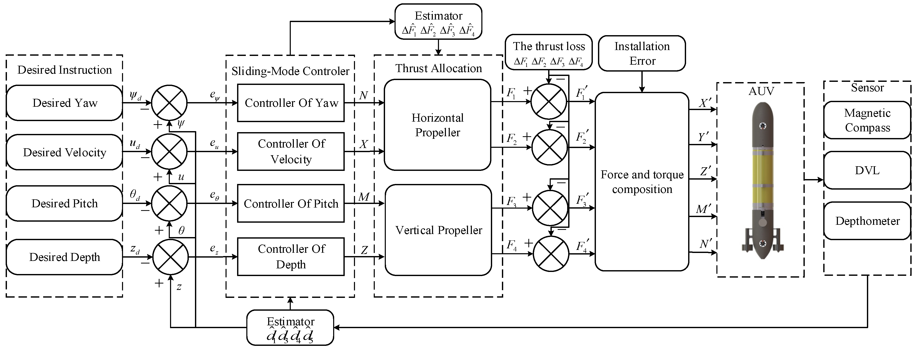
The influence of thruster misalignment and thrust loss on the motion control of AUV is particularly obvious in fully thruster-driven AUV carriers, as shown in Figure 1. The horizontal actuators of the AUV are the two main thrusters on the left and right sides, respectively, to control the speed and yaw of AUV. The vertical actuator consists of two tunnel thrusters on the forward and back of AUV, respectively, which can control the depth and pitch. It belongs to a typical multi-thruster-drive AUV.

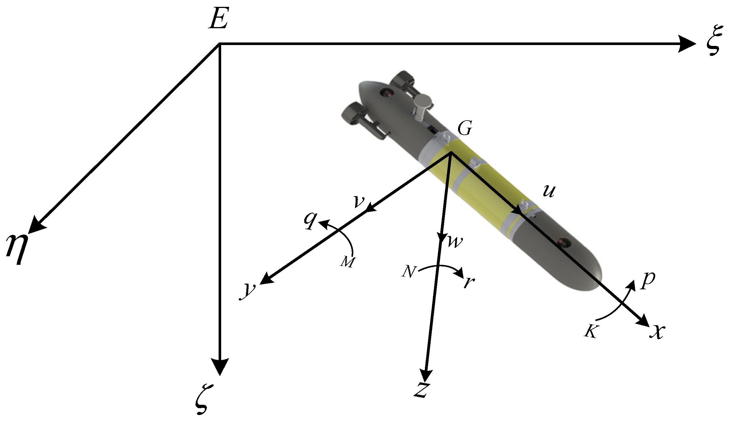
According to ITTC recommendation and SNAME Terminology Bulletin System [18], the co-ordinate system, as shown in Figure 2, is established with reference to relevant literature.

The kinematics and dynamics equations of AUV six freedoms are as follows [19]:

$$\dot{\mathsf{\eta }} =\mathbf{J}(\mathsf{\eta })\mathbf{v}$$

(1)

$$\mathbf{M} \dot{\mathbf{v}} +\mathbf{C}(\mathbf{v})\mathbf{v}+\mathbf{D}(\mathbf{v})\mathbf{v}+\mathbf{g}(\mathsf{\eta })+{\mathsf{\tau }}_{\mathbf{d}}=\mathsf{\tau }$$

(2)

where, $\mathbf{v}={\left[\begin{array}{cccccc}u& v& w& p& q& r\end{array}\right]}^T$ is the velocity vector of AUV in the body co-ordinate system, $\mathsf{\eta }={\left[\begin{array}{cccccc}x& y& z& \phi & \theta & \psi \end{array}\right]}^T$ is the position and attitude angle vector of AUV in the earth co-ordinate system, $\mathbf{J}(\mathsf{\eta })$ is the co-ordinate transformation matrix, $\mathsf{\tau }={\left[\begin{array}{cccccc}{T}_x& T_y& T_z& M_x& M_y& M_z\end{array}\right]}^T$ is the force and moment generated by the thruster, and ${\mathsf{\tau }}_{\mathbf{d}}={\left[\begin{array}{cccccc}{\tau }_{eu}& {\tau }_{ev}& {\tau }_{ew}& {\tau }_{ep}& {\tau }_{eq}& {\tau }_{er}\end{array}\right]}^T$ is the disturbance force and moment. $\mathbf{M}$ is the is the rigid-body inertia matrix, $\mathbf{C}(\mathbf{v})$ is a matrix of rigid-body Coriolis and centripetal forces, $\mathbf{D}(\mathbf{v})$ is the damping force matrix, and $\mathbf{g}(\mathsf{\eta })$ is the generalized gravity and buoyancy vector. In the study of this paper, gravity is equal to buoyancy. The kinematics and dynamics equations of the above matrix form are expanded without considering the rolling motion of AUV, so the following can be obtained.

The kinematic equation of AUV is:

$$\{\begin{array}{c}\dot{x}=u\cos \psi \cos \theta -v\sin \psi +w\cos \psi \sin \theta \hfill \\ \dot{y}=u\sin \psi \cos \theta +v\cos \psi +w\sin \psi \sin \theta \hfill \\ \dot{z}=-u\sin \theta +w\cos \theta \hfill \\ \dot{\theta }=q\hfill \\ \dot{\psi }=r/\cos \theta \hfill \end{array}$$

(3)

The dynamic equation of AUV is:

$$\{\begin{array}{cc}\hfill (m-X_{\dot{u}})\dot{u}& =X+X_{uu}{u}^2+X_{vv}{v}^2+X_{ww}{w}^2+X_{qq}{q}^2+{\tau }_{eu}\hfill \\ \hfill (m-Y_{\dot{v}})\dot{v}& =-(m-Y_{ur})ur+Y_{v}uv+Y_{v\left|v\right|}v\left|v\right|+{\tau }_{ev}\hfill \\ \hfill (m-Z_{\dot{w}})\dot{w}& =Z-(m-Z_{uq})uq+Z_{uw}uw+Z_{w\left|w\right|}w\left|w\right|+m{z}_g{q}^2+{\tau }_{ew}\hfill \\ \hfill (I_y-M_{\dot{q}})\dot{q}& =M+M_{q\left|q\right|}q\left|q\right|-M_{uq}uq-M_{uw}uw-\hfill \\ & (z_{g}w-z_{b}B)\sin \theta -m{z}_g(wq-vr)+{\tau }_{eq}\hfill \\ \hfill (I_z-N_{\dot{r}})\dot{r}& =N+N_{uv}uv+N_{v\left|v\right|}v\left|v\right|+N_{ur}ur+{\tau }_{er}\hfill \end{array}$$

(4)

where, $X,Z,M,N$ is the control force and moment, ${\tau }_{eu},{\tau }_{ev},{\tau }_{ew},{\tau }_{eq},{\tau }_{er}$ is the bounded time-varying interference force or moment, $X_{(\cdot )},Y_{(\cdot )},Z_{(\cdot )},M_{(\cdot )},N_{(\cdot )}$ is the hydrodynamic parameters of AUV, m is the mass of AUV, I_x, I_y, I_z is the moment of inertia of AUV rotating around the three axes of the body co-ordinate system, and $z_g,z_b$ is the vertical position of AUV center of gravity and center of buoyancy. The values of the above symbols in this article are shown in

Table 1. Main parameters of AUV-R.

Shape Parameters	$m=44.1\mathrm{kg}$	$I_y=8.0980\mathrm{kg}\cdot {\mathrm{m}}^2$	$I_z=8.0670\mathrm{kg}\cdot {\mathrm{m}}^2$
	$L=1.46\mathrm{m}$	$d=0.21\mathrm{m}$	$z_b=0,z_g=0.0187$
Hydrodynamic Parameters	$X_{\dot{u}}=-2.52\mathrm{kg}$	$X_{uu}=-6.44\mathrm{kg}/\mathrm{m}$	$X_{rr}=-2.29\mathrm{kg}\cdot \mathrm{m}/\mathrm{rad}$
	$X_{ww}=0\mathrm{kg}/\mathrm{m}$	$M_{\dot{q}}=-5.43\mathrm{kg}\cdot {\mathrm{m}}^2$	$X_{qq}=-2.29\mathrm{kg}\cdot \mathrm{m}/\mathrm{rad}$
	$Y_{\dot{v}}=-49.05\mathrm{kg}$	$Y_{ur}=35.41\mathrm{kg}/\mathrm{rad}$	$Z_{uw}=-46.65\mathrm{kg}/\mathrm{rad}$
	$M_{uw}=16.43\mathrm{kg}$	$N_{\dot{r}}=-5.31\mathrm{kg}\cdot {\mathrm{m}}^2$	$M_{uq}=-23.76\mathrm{kg}\cdot \mathrm{m}/\mathrm{rad}$
	$X_{vv}=0\mathrm{kg}/\mathrm{m}$	$Z_{w\left|w\right|}=-141.66\mathrm{kg}/\mathrm{m}$	$N_{ur}=-27.2\mathrm{kg}\cdot {\mathrm{m}}^2/(\mathrm{s}\cdot \mathrm{rad})$
	$N_{uv}=-14.99\mathrm{kg}$	$Y_{v\left|v\right|}=-194.77\mathrm{kg}/\mathrm{m}$	$M_{q\left|q\right|}=-3.98\mathrm{kg}\cdot {\mathrm{m}}^2/{\mathrm{rad}}^2$
	$N_{v\left|v\right|}=11.00\mathrm{kg}$	$Y_v=-44.96\mathrm{kg}/\mathrm{s}$
	$Z_{\dot{w}}=-49.12\mathrm{kg}$	$Z_{uq}=-27.27\mathrm{kg}/\mathrm{rad}$

.

In the process of AUV motion control, the calculated control force is distributed to each thruster through the nominal thrust distribution matrix $\mathbf{H}$. However, due to thruster misalignment, the thruster output forces applied to the AUV do not match the desired force and moment. When thruster misalignment exists, the uncertainty matrix of the nominal control distribution matrix generated by thruster misalignment is ${\mathbf{H}}_{\Delta }$, and the pseudo-inverse method is used for control distribution. When thruster misalignment exists, the actual force acting on AUV is:

$${\mathbf{T}}^{\prime }={\mathbf{H}}^{-1}\mathbf{T}{\mathbf{H}}_{\Delta }$$

(5)

where, $\mathbf{T}={\left[\begin{array}{ccccc}X& 0& Z& M& N\end{array}\right]}^T$ is the control force output vector of the controller and ${\mathbf{T}}^{\prime }$ is the force vector actually acted on the AUV carrier. In this paper:

$$\mathbf{H}=\left[\begin{array}{cccc}1& 1& 0& 0\\ 0& 0& 0& 0\\ 0& 0& 1& 1\\ 0& 0& -0.654& 0.8\\ 0.187& -0.187& 0& 0\end{array}\right]$$

(6)

When the thruster misalignment exists, the deviation angles of the two main thrusters from the positive direction of the x-axis in the xoy plane are ${\gamma }_1$ and ${\gamma }_2$, respectively, and the deviation angles with the xoy plane are ${\gamma }_3$ and ${\gamma }_4$, respectively, and the installation position deviation in the x-axis, y-axis, and z-axis direction is $l_i$ (where $i=1,2,3$ is the left main thruster; where $i=4,5,6$ is the right main thruster). The deviation angles of the forward and backward vertical thruster from the positive direction of z-axial direction are ${\gamma }_5$ and ${\gamma }_6$, respectively, and the deviation angles from the positive direction of x-axial direction in the xoy plane are ${\gamma }_7$ and ${\gamma }_8$, respectively, and the installation position deviation of the x-axis, y-axis, and z-axis direction is $l_i$ (where $i=7,8,9$ is the forward tunnel thrusters; where $i=10,11,12$ is the back tunnel thrusters). Where ${\gamma }_i$($i=1,2,\cdots 8$) is positive in the positive direction of each co-ordinate axis to the right, $l_i$ ($i=1,2,\cdots 12$) is positive when it is the same as the positive direction of each co-ordinate axis; then, the distribution matrix in case of installation deviation is:

$${\mathbf{H}}_{\Delta }=\left[\begin{array}{cccc}\cos {\gamma }_3\cos {\gamma }_1& \cos {\gamma }_4\cos {\gamma }_2& \sin {\gamma }_5\cos {\gamma }_7& \sin {\gamma }_6\cos {\gamma }_8\\ \cos {\gamma }_3\sin {\gamma }_1& \cos {\gamma }_4\sin {\gamma }_2& \sin {\gamma }_5\sin {\gamma }_7& \sin {\gamma }_6\sin {\gamma }_8\\ \sin {\gamma }_3& \sin {\gamma }_4& \cos {\gamma }_5& \cos {\gamma }_6\\ E_1& E_2& E_3& E_4\\ E_5& E_6& E_7& E_8\end{array}\right]$$

(7)

In Equation (7), $E_i$($i=1,2\cdots 8$) is equal to:

$$\begin{array}{l}{E}_1=(0.907-l_1)\sin {\gamma }_3\\ E_2=(0.907-l_4)\sin {\gamma }_4\\ E_3=-(0.654+l_7)\cos {\gamma }_5\\ E_4=(0.8-l_{10})\cos {\gamma }_6\\ E_5=(0.187-l_2)\cos {\gamma }_3\cos {\gamma }_1-(0.907-l_1)\cos {\gamma }_3\sin {\gamma }_1\\ E_6=-(0.187+l_5)\cos {\gamma }_4\cos {\gamma }_2-(0.907-l_1)\cos {\gamma }_4\sin {\gamma }_2\\ E_7=-l_8\sin {\gamma }_5\cos {\gamma }_7+(0.654+l_7)\sin {\gamma }_5\sin {\gamma }_7\\ E_8=-l_{11}\sin {\gamma }_6\cos {\gamma }_8-(0.8-l_{10})\sin {\gamma }_6\sin {\gamma }_8\end{array}$$

(8)

When there is no thruster misalignment, ${\gamma }_i=0$ ($i=1,2,\cdots 8$) and $l_i=0$ ($i=1,2,\cdots 12$), then $\mathbf{H}={\mathbf{H}}_{\Delta }$. In addition to consideration of thruster misalignment, this paper also considers the thrust loss of the thruster. Assume that the forces of the thrusters are $\mathbf{F}={\left[\begin{array}{cccc}{F}_1& F_2& F_3& F_4\end{array}\right]}^T$, and the thrust loss is ${\Delta }_T={\left[\begin{array}{cccc}\Delta F_1& \Delta F_2& \Delta F_3& \Delta F_4\end{array}\right]}^T$, then:

$${\mathbf{F}}^{\prime }=\mathbf{F}-{\Delta }_T$$

(9)

${\Delta }_T$ will increase as $\mathbf{F}$ increases. If $\mathbf{F}=0$, ${\Delta }_T=0$. When $\mathbf{F}\ne 0$, the true force and moment of AUV are:

$${\mathbf{T}}^{\prime }=({\mathbf{H}}^{-1}\mathbf{T}-{\Delta }_T){\mathbf{H}}_{\Delta }$$

(10)

In order to verify the effect of thruster misalignment and thrust loss on AUV motion control, take $l_i=0.02$ ($i=1,2\cdots 12$), ${\gamma }_1={\gamma }_3={\gamma }_5={\gamma }_7=-\frac{3\pi }{90}$, ${\gamma }_2={\gamma }_4={\gamma }_6={\gamma }_8=\frac{5\pi }{90}$, $u_d=0.5\mathrm{m}/\mathrm{s}$, ${\psi }_d=60°$, $z_d=10\mathrm{m}$, ${\theta }_d=0°$ for simulation test and the results are shown from Figure 3, Figure 4, Figure 5 and Figure 6:

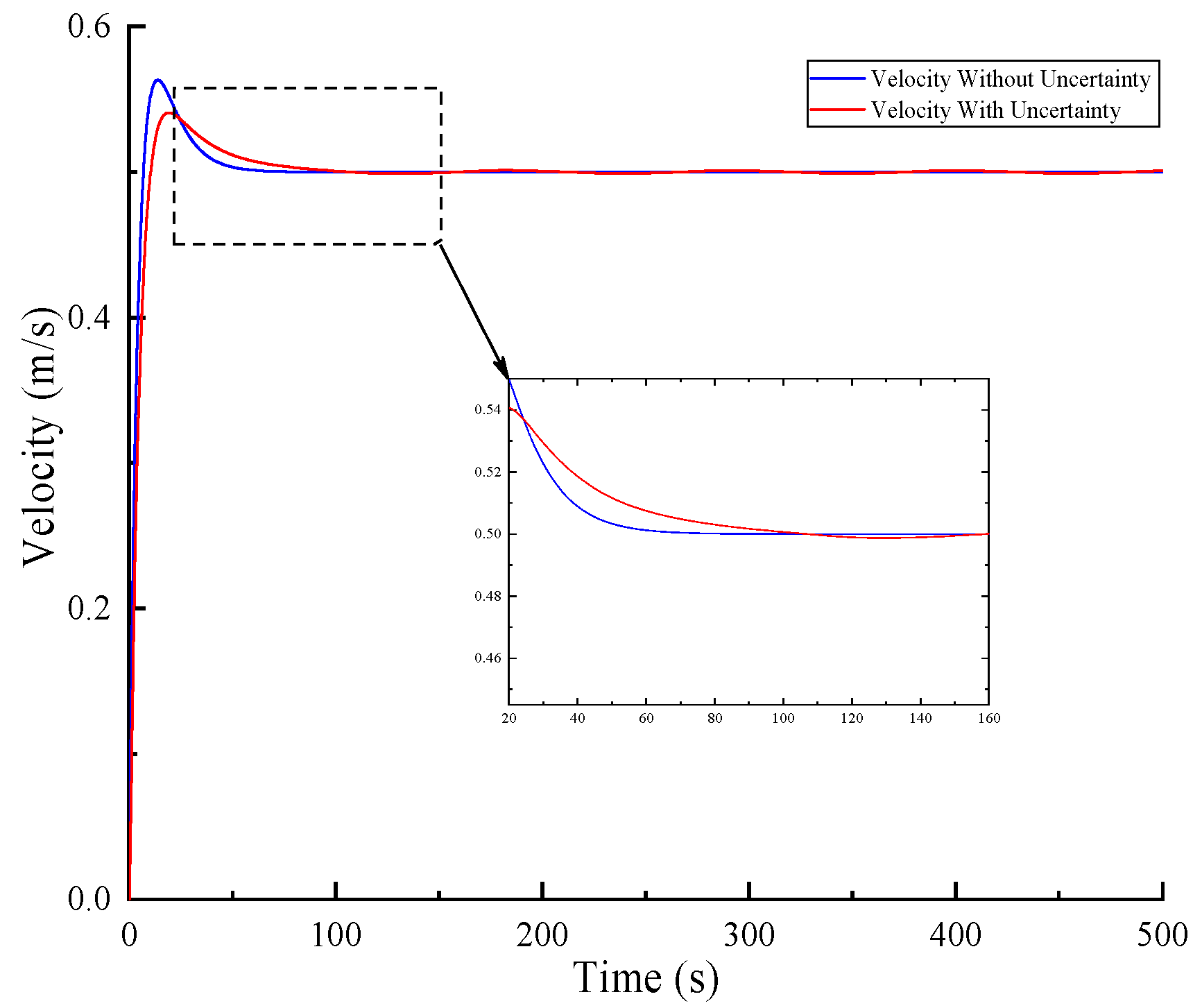
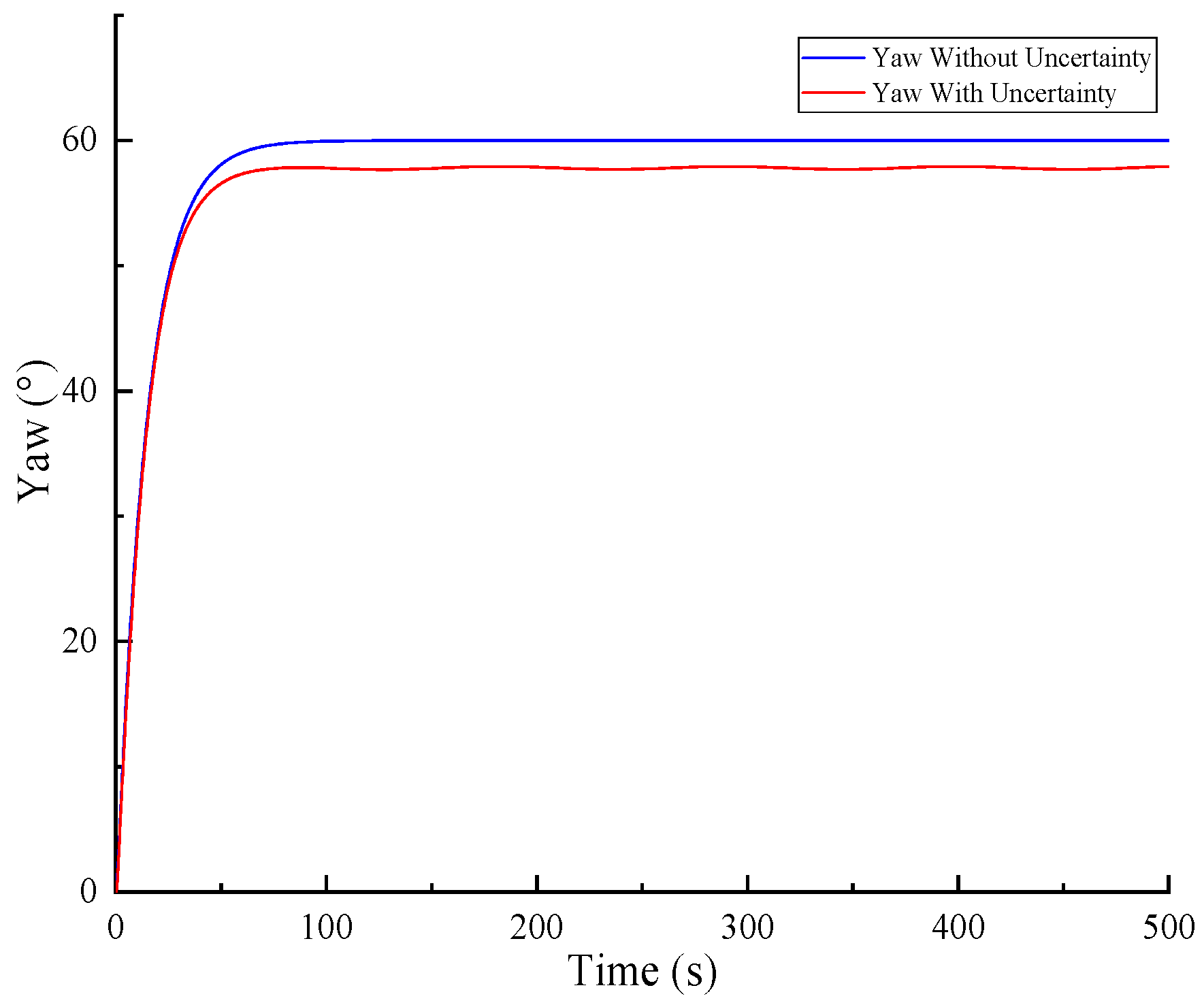
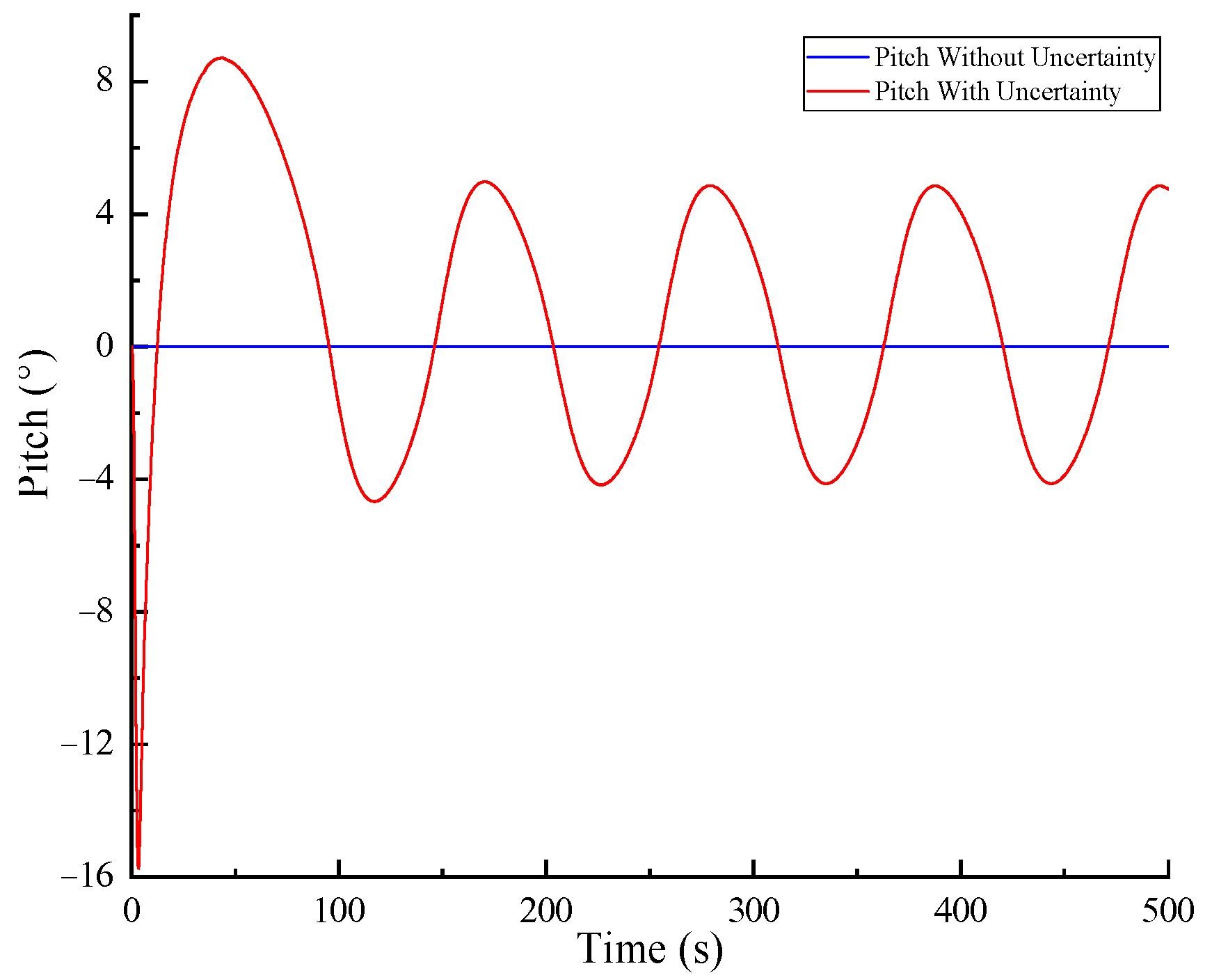
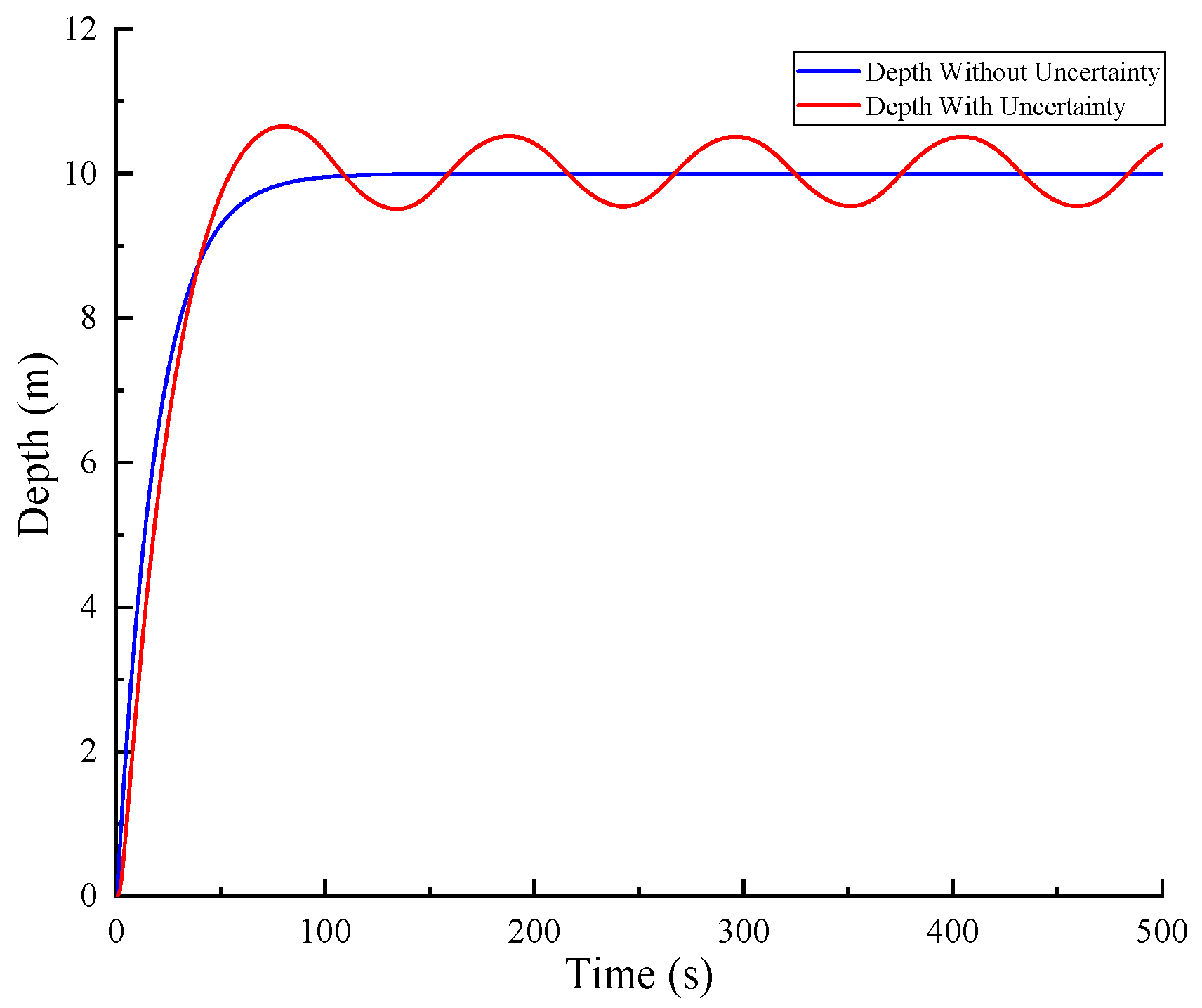
It can be seen from Figure 3, Figure 4, Figure 5 and Figure 6, when there is thruster misalignment and thrust loss, the velocity control is stable slowly, and the yaw control has $2^{\circ }$ steady-state error that cannot be eliminated. The pitch control appears to possess a larger fluctuation maximum to $-{15}^{\circ }$, with a minimum fluctuation between $-5\sim 5^{\circ }$, and it cannot gain stability. The depth control also has a big fluctuation, with the maximum exceeding the desired depth of 0.6 m. It can be seen that thruster misalignment and thrust loss have a great impact on the motion control effect of AUV.

3. Controller Design

In this paper, two observers are designed to compensate the force and moment deviation caused by thruster misalignment and thrust loss. The principle of the designed controller is shown in Figure 7.

To facilitate the design of the disturbance observer, Formula (4) is deformed and considers the deviation of force and moment caused by thruster misalignment. Then:

$$\{\begin{array}{c}\dot{u}=\frac{X}{m_u}+\frac{X_{uu}}{m_u}{u}^2+\frac{X_{vv}}{m_u}{v}^2+\frac{X_{ww}}{m_u}{w}^2+\frac{X_{qq}}{m_u}{q}^2+\frac{{\tau }_{eu}}{m_u}\hfill \\ \dot{v}=-\frac{m_{ur}}{m_v}ur+\frac{Y_v}{m_v}uv+\frac{Y_{v\left|v\right|}}{m_v}v\left|v\right|+\frac{{\tau }_{ev}}{m_v}\hfill \\ \dot{w}=\frac{Z}{m_w}-\frac{m_{uq}}{m_w}uq+\frac{Z_{uw}}{m_w}uw+\frac{Z_{w\left|w\right|}}{m_w}w\left|w\right|+\frac{{\tau }_{ew}}{m_w}\hfill \\ \dot{q}=\frac{M}{m_q}+\frac{M_{q\left|q\right|}}{m_q}q\left|q\right|-\frac{M_{uq}}{m_q}uq-\frac{M_{uw}}{m_q}uw+\frac{{\tau }_{eq}}{m_q}-\hfill \\ \hspace{1em}\frac{(z_{g}w-z_{b}B)\sin \theta -m{z}_g(wq-vr)}{m_q}\hfill \\ \dot{r}=\frac{N}{m_r}+\frac{N_{uv}}{m_r}uv+\frac{N_{v\left|v\right|}}{m_r}v\left|v\right|+\frac{N_{ur}}{m_r}ur+{\tau }_{er}\hfill \end{array}$$

(11)

where:

$$\begin{array}{l}{m}_u=m-X_{\dot{u}},m_v=m-Y_{\dot{v}},m_w=m-Z_{\dot{u}}\\ m_{ur}=m-Y_{ur},m_{uq}=m-Z_{uq}\\ m_r=I_z-N_{\dot{r}},m_q=I_y-M_{\dot{q}}\end{array}$$

Equation (11) can be rewritten into the equation of state in the form:

$$\{\begin{array}{l}\dot{u}=f_1+g_{1}X+d_1\\ \dot{v}=f_2+d_2\\ \dot{w}=f_3+g_{3}Z+d_3\\ \dot{q}=f_4+g_{4}M+d_4\\ \dot{r}=f_5+g_{5}N+d_5\end{array}$$

(12)

where:

$$f_1=\frac{X_{uu}}{m_u}{u}^2+\frac{X_{vv}}{m_u}{v}^2+\frac{X_{ww}}{m_u}{w}^2+\frac{X_{qq}}{m_u}{q}^2$$

$$f_2=-\frac{m_{ur}}{m_v}ur+\frac{Y_v}{m_v}uv+\frac{Y_{v\left|v\right|}}{m_v}v\left|v\right|$$

$$f_3=-\frac{m_{uq}}{m_w}uq+\frac{Z_{uw}}{m_w}uw+\frac{Z_{w\left|w\right|}}{m_w}w\left|w\right|$$

$$f_4=\frac{M_{q\left|q\right|}}{m_q}q\left|q\right|-\frac{M_{uq}}{m_q}uq-\frac{M_{uw}}{m_q}uw$$

$$f_5=\frac{N}{m_r}+\frac{N_{uv}}{m_r}uv+\frac{N_{v\left|v\right|}}{m_r}v\left|v\right|+\frac{N_{ur}}{m_r}ur$$

$$g_1=\frac{1}{m_u},g_3=\frac{1}{m_w},g_4=\frac{1}{m_q},g_5=\frac{1}{m_r}$$

$$d_1={\tau }_{eu},d_2={\tau }_{ev},d_3={\tau }_{ew},d_4={\tau }_{eq},d_5={\tau }_{er}$$

In the three-dimensional motion control of AUV, velocity, yaw, depth, and pitch are controlled, so the velocity control law, depth control law, pitch control law, and yaw control law should be designed so that:

$$\underset{t\to \infty }{\lim }(u-u_d)=0,\underset{t\to \infty }{\lim }(\psi -{\psi }_d)=0,\underset{t\to \infty }{\lim }(\theta -{\theta }_d)=0,\underset{t\to \infty }{\lim }(z-z_d)=0$$

Define the error as:

$$\begin{array}{l}{e}_u=u-u_d\\ e_{\psi }=\psi -{\psi }_d\\ e_z=z-z_d\\ e_{\theta }=\theta -{\theta }_d\end{array}$$

(13)

where, $u_d$ is the desired speed, ${\psi }_d$ is the desired yaw, $z_d$ is the desired depth, and ${\theta }_d$ is the desired pitch.

The sliding mode surface is defined as:

$$\begin{array}{l}{S}_1=e_u+k_u{\displaystyle {\int }_0^t{e}_u}dt\\ S_2=k_{\psi }{e}_{\psi }+{\dot{e}}_{\psi }\\ S_3=k_z{e}_z+{\dot{e}}_z\\ S_4=k_{\theta }{e}_{\theta }+{\dot{e}}_{\theta }\end{array}$$

(14)

where, $k_u,k_{\psi },k_z,k_{\theta }>0$ is the parameters of sliding mode surface. Define the Lyapunov function as:

$$V_1=\frac{1}{2}(S_1{}^2+S_2{}^2+S_3{}^2+S_4{}^2)$$

(15)

The derivative of Equation (15) can be obtained:

$${\dot{V}}_1=S_1{\dot{S}}_1+S_2{\dot{S}}_2+S_3{\dot{S}}_3+S_4{\dot{S}}_4$$

(16)

In order to reduce jitter in the sliding mode controller, the following convergence law is adopted:

$$\begin{array}{l}{\dot{S}}_1=-k_1\tanh (S_1)-k_2{S}_1\\ {\dot{S}}_2=-k_3\tanh (S_2)-k_4{S}_2\\ {\dot{S}}_3=-k_5\tanh (S_3)-k_6{S}_3\\ {\dot{S}}_4=-k_7\tanh (S_4)-k_8{S}_4\end{array}$$

(17)

where $k_i>0$ ($i=1,2,\cdots 8$) is the parameters of the sliding mode controller.

Substitute Equation (16) into Equation (17) to obtain:

$$\begin{array}{cc}\hfill {\dot{V}}_1& =S_1(-k_1\tanh (S_1)-k_2{S}_1)+S_2(-k_3\tanh (S_2)-k_4{S}_2)\hfill \\ & +S_3(-k_5\tanh (S_3)-k_6{S}_3)+S_4(-k_7\tanh (S_4)-k_8{S}_3)\hfill \\ & =-k_1\tanh (S_1)S_1-k_3\tanh (S_2)S_2-k_5\tanh (S_3)S_3-k_7\tanh (S_4)S_4\hfill \\ & -k_2{S}_1{}^2-k_4{S}_2{}^2-k_6{S}_3{}^2-k_8{S}_4{}^2\hfill \end{array}$$

(18)

Since the hyperbolic tangent function is odd function, the velocity error, yaw error, depth error, and pitch error are gradually stable. According to Equation (14), we can obtain:

$$\begin{array}{l}{\dot{S}}_1={\dot{e}}_u+k_u{e}_u\\ {\dot{S}}_2=k_{\psi }{\dot{e}}_{\psi }+{\ddot{e}}_{\psi }\\ {\dot{S}}_3=k_z{\dot{e}}_z+{\ddot{e}}_z\\ {\dot{S}}_4=k_{\theta }{\dot{e}}_{\theta }+{\ddot{e}}_{\theta }\end{array}$$

(19)

According Equation (13), Equation (19) can be rewritten as:

$$\begin{array}{l}{\dot{S}}_1=\dot{u}+k_u{e}_u\\ {\dot{S}}_2=k_{\psi }r+\dot{r}\\ {\dot{S}}_3=k_z\dot{z}+\dot{w}\\ {\dot{S}}_4=k_{\theta }\dot{\theta }+\dot{q}\end{array}$$

(20)

According to Equations (17) and (20), we can obtain:

$$\begin{array}{l}\dot{u}=-k_1\tanh (S_1)-k_2{S}_1-k_u{e}_u\\ \dot{r}=-k_3\tanh (S_2)-k_4{S}_2-k_{\psi }r\\ \dot{q}=-k_7\tanh (S_4)-k_8{S}_4-k_{\theta }q\\ \dot{w}=\frac{1}{\cos \theta }(-k_5\tanh (S_3)-k_6{S}_3-k_z{\dot{e}}_z+\dot{u}\sin \theta -uq\cos \theta +wq\sin \theta )\end{array}$$

(21)

Then, the control force of AUV is:

$$\{\begin{array}{l}X=m_u(-k_1\tanh (S_1)-k_2{S}_1-k_u{e}_u)+d_u-d_1\\ Z=\frac{m_W}{\cos \theta }(-k_5\tanh (S_3)-k_6{S}_3-k_z{\dot{e}}_z+\dot{u} \sin \theta -uq\cos \theta +wq\sin \theta )+d_w-d_3\\ M=m_q(-k_7\tanh (S_4)-k_8{S}_4-k_{\theta }q)+d_q-d_4\\ N=m_r(-k_3\tanh (S_2)-k_4{S}_2-k_{\psi }r)+d_r-d_5\end{array}$$

(22)

where:

$$d_u=-X_{uu}{u}^2-X_{vv}{v}^2-X_{ww}{w}^2-X_{qq}{q}^2$$

$$d_w=-Z_{uw}uw-Z_{w\left|w\right|}w\left|w\right|-m{z}_g{q}^2$$

$$d_r=-N_{uv}uv-N_{v\left|v\right|}v\left|v\right|-N_{ur}ur$$

$$d_q=-M_{q\left|q\right|}q\left|q\right|+M_{uq}uq+M_{uw}uw+(z_{g}w-z_{b}B)\sin \theta +m{z}_g(wq-vr)$$

In Equation (22), $d_i$($i=1,3,4,5$) is unknown and increases with the increase in control force. Therefore, the observer is designed to estimate the disturbance. This gives the following theorem:

Theorem 1.

For the following system:

$$\{\begin{array}{l}{\dot{x}}_1=x_2\\ {\dot{x}}_2=-a_1{\left|x_1\right|}^b\arctan (x_1)-a_2{\left|x_2\right|}^b\arctan (x_2)\end{array}$$

(23)

Define the Lyapunov function as follows:

$$V_2={\displaystyle {\int }_0^{x_1}{a}_1{\left|x_1\right|}^b}\arctan (\xi )d\xi +\frac{1}{2}{x}_2{}^2$$

(24)

The derivative of Equation (24) can be obtained:

$$\begin{array}{cc}\hfill \dot{V}{ }_2& =a_1{\dot{x}}_1 {\left|x_1\right|}^b\arctan (x_1)+x_2{\dot{x}}_2 \hfill \\ & =a_1{x}_2{\left|x_1\right|}^b\arctan (x_1)+x_2(-a_1{\left|x_1\right|}^b\arctan (x_1)-a_2{\left|x_2\right|}^b\arctan (x_2))\hfill \\ & =-a_2{x}_2{\left|x_2\right|}^b\arctan (x_2)\le 0\hfill \end{array}$$

(25)

Therefore, when $a_1>0$, $a_2>0$, $x_1\in R$, $x_2\in R$, the system is asymptotically stable at $(0,0)$.

Lemma 1.

For the following systems:

$$\{\begin{array}{l}{\dot{x}}_1=x_2\\ {\dot{x}}_2=F(x_1,x_2)\end{array}$$

(26)

where$x_1\in R$,$x_2\in R$,$F(\cdot ):R^2\to R$. If the solution of Equation (26) satisfies$x_1(t)\to 0$,$x_2(t)\to 0(t\to \infty )$, then, for any bounded and integrable function$v(t)$, and$T>0$,$R>0$, the solution of the following system:

$$\{\begin{array}{l}{\dot{x}}_1=x_2\\ {\dot{x}}_2=R^{2}F(x_1-v(t),x_2/R)\end{array}$$

(27)

satisfies:

$$\underset{R\to \infty }{\lim }{\displaystyle {\int }_0^T\left|x_1(t)-v(t)\right|dt=0}$$

(28)

That is, the generalized derivative of $x_1(t)$ converges $v(t)$ on average; $x_2(t)$ weakly converges on $v(t)$. According to Lemma 1 and Theorem 1, the following disturbance estimators are designed:

$$\{\begin{array}{l}\dot{\widehat{u}}=\frac{X}{m_u}+\frac{X_{uu}}{m_u}{u}^2+\frac{X_{vv}}{m_u}{v}^2+\frac{X_{ww}}{m_u}{w}^2+\frac{X_{qq}}{m_u}{q}^2+\frac{{\widehat{d}}_1}{m_u}\\ {\dot{\widehat{d}}}_1=R_1{}^2\left[-L_1{\left|\widehat{u}-u\right|}^{b_1}\arctan (\widehat{u}-u)-L_2{\left|{\widehat{d}}_1/R_1\right|}^{b_1}\arctan ({\widehat{d}}_1/R_1)\right]\end{array}$$

(29)

$$\{\begin{array}{l}\dot{\widehat{w}}=\frac{Z}{m_w}-\frac{m_{uq}}{m_w}uq+\frac{Z_{uw}}{m_w}uw+\frac{Z_{w\left|w\right|}}{m_w}w\left|w\right|+\frac{{\widehat{d}}_3}{m_w}\\ {\dot{\widehat{d}}}_3=R_3{}^2\left[-L_3{\left|\widehat{w}-w\right|}^{b_3}\arctan (\widehat{w}-w)-L_4{\left|{\widehat{d}}_3/R_3\right|}^{b_3}\arctan ({\widehat{d}}_3/R_3)\right]\end{array}$$

(30)

$$\{\begin{array}{l}\dot{\widehat{\theta }}=\widehat{q}\\ \dot{\widehat{q}}=\frac{M}{m_q}+\frac{M_{q\left|q\right|}}{m_q}q\left|q\right|-\frac{M_{uq}}{m_q}uq-\frac{M_{uw}}{m_q}uw+\frac{{\widehat{d}}_4}{m_q}\\ {\dot{\widehat{d}}}_4=R_4{}^2\left[-L_5{\left|\widehat{\theta }-\theta \right|}^{b_4}\arctan (\widehat{\theta }-\theta )-L_6{\left|{\widehat{d}}_4/R_4\right|}^{b_4}\arctan ({\widehat{d}}_4/R_4)\right]\end{array}$$

(31)

$$\{\begin{array}{l}\dot{\widehat{\psi }}=\widehat{r}\\ \dot{\widehat{r}}=\frac{N}{m_r}+\frac{N_{uv}}{m_r}uv+\frac{N_{v\left|v\right|}}{m_r}v\left|v\right|+\frac{N_{ur}}{m_r}ur+\frac{{\widehat{d}}_5}{m_r}\\ {\dot{\widehat{d}}}_{ 5}=R_5{}^2\left[-L_7{\left|\widehat{\psi }-\psi \right|}^{b_5}\arctan (\widehat{\psi }-\psi )-L_8{\left|{\widehat{d}}_5/R_5\right|}^{b_5}\arctan ({\widehat{d}}_5/R_5)\right]\end{array}$$

(32)

When $T>0$ and $R_i>0$ ($i=1,3,4,5$):

$$\{\begin{array}{l}\underset{R_1\to \infty }{\lim }{\displaystyle {\int }_0^T\left|\widehat{u}-u\right|dt=0}\\ \underset{R_3\to \infty }{\lim }{\displaystyle {\int }_0^T\left|\widehat{w}-w\right|dt=0}\\ \underset{R_4\to \infty }{\lim }{\displaystyle {\int }_0^T\left|\widehat{\theta }-\theta \right|dt=0}\\ \underset{R_5\to \infty }{\lim }{\displaystyle {\int }_0^T\left|\widehat{\psi }-\psi \right|dt=0}\end{array}$$

(33)

From the above formula, we can know:

$$\{\begin{array}{l}\widehat{u}\to u\\ \widehat{w}\to w\\ \widehat{\theta }\to \theta \\ \widehat{\psi }\to \psi \end{array}$$

(34)

From ${\widehat{d}}_1-d_1=\widehat{u}-u$, ${\widehat{d}}_3-d_3=\widehat{w}-w$, ${\widehat{d}}_4-d_4=\widehat{q}-q$,${\widehat{d}}_5-d_5=\widehat{r}-r$, we can obtain:

$$\{\begin{array}{l}{\widehat{d}}_1\to d_1\\ {\widehat{d}}_3\to d_3\\ {\widehat{d}}_4\to d_4\\ {\widehat{d}}_5\to d_5\end{array}$$

(35)

Let the state estimation error and the disturbance estimation error be:

$$\begin{array}{l}\tilde{u}=\widehat{u}-u,\tilde{w}=\widehat{w}-w,\tilde{\theta }=\widehat{\theta }-\theta ,\tilde{\psi }=\widehat{\psi }-\psi \\ {\tilde{d}}_1={\widehat{d}}_1-d_1,{\tilde{d}}_3={\widehat{d}}_3-d_3,{\tilde{d}}_4={\widehat{d}}_4-d_4,{\tilde{d}}_5={\widehat{d}}_5-d_5\end{array}$$

(36)

According to Equations (34) and (35), state estimation error and disturbance estimation error converge.

The thrust distribution of the control force can be obtained:

$$\left[\begin{array}{cccc}1& 1& 0& 0\\ 0& 0& 0& 0\\ 0& 0& 1& 1\\ 0& 0& -0.654& 0.8\\ 0.187& -0.187& 0& 0\end{array}\right]\left[\begin{array}{c}X\\ 0\\ Z\\ M\\ N\end{array}\right]=\left[\begin{array}{c}{F}_1\\ F_2\\ F_3\\ F_4\end{array}\right]$$

(37)

The calculation formula of thruster thrust can also be obtained from AUV hydrodynamic test:

$$F_i=C_n{n}_i\left|n_i\right|$$

(38)

where $F_i$($i=1,2,3,4$) is the thrust of the four thrusters and $n_i$($i=1,2,3,4$) is the speed of the four thrusters. At the same time, the thruster system has thrust loss due to the instability of incoming flow and the existence of model error. Therefore, a nonlinear state observer is designed to estimate the thrust loss. The differential equation describing thrust loss can be expressed as:

$${\dot{\Delta }}_T{}^i=-\frac{1}{{\tau }_i}{\Delta }_T{}^i+w_i$$

(39)

where ${\tau }_i$($i=1,2,3,4$) represents time constant, $w_i$($i=1,2,3,4$) represents bounded noise, and ${\Delta }_T{}^i$($i=1,2,3,4$) represents the thrust of four thrusters. It is very difficult to obtain an accurate model because of unknown flow velocity and unsteady flow disturbance of the thruster, but this model is often used to estimate unknown variables. The equation of thruster dynamics can be written as:

$$2\pi J_m{}^i\dot{n}=Q_m{}^i-Q_p{}^i-2\pi K_n{}^i{n}_i$$

(40)

where $n_i$($i=1,2,3,4$) is thruster speed, $J_m{}^i$($i=1,2,3,4$) is thruster moment of inertia, $K_n{}^i$($i=1,2,3,4$) is linear damping coefficient, $Q_m{}^i$($i=1,2,3,4$) is motor command moment, $Q_p{}^i$($i=1,2,3,4$) is thruster moment, and ${\Delta }_T{}^i$($i=1,2,3,4$) represents thrust loss. From $Q_p{}^i=K_1{n}_i{}^2+K_2{\Delta }_T{}^i$, we can obtain:

$$2\pi J_m{}^i{\dot{n}}_i=Q_m{}^i-K_1{n}_i{}^2-K_2{\Delta }_T{}^i-2\pi K_n{}^i{n}_i$$

(41)

Command moment of the motor is:

$$Q_m{}^i=\frac{D_i{K}_Q{}^i}{K_T{}^i}{T}_{pd}{}^i$$

(42)

The observer is designed according to Equations (23) and (25), and the system output is expressed as $y_i=n_i$, $K_1>0$, $K_2>0$. Assuming nonlinear gain, $p$ and $m$ are used to estimate thrust loss:

$$\{\begin{array}{l}2\pi J_m{}^i{\dot{\widehat{n}}}_i=Q_m{}^i-K_1{\widehat{n}}_i{}^2-K_2{\widehat{\Delta }}_T{}^i-2\pi K_n{}^i{\widehat{n}}_i+p_i(y_i-{\widehat{y}}_i)\\ {\dot{\widehat{\Delta }}}_T{}^i=-\frac{1}{{\tau }_i}{\Delta }_T{}^i+m_i(y_i-{\widehat{y}}_i)\end{array}$$

(43)

Let ${\tilde{n}}_i=n_i-{\widehat{n}}_i$, ${\tilde{\Delta }}_T{}^i={\Delta }_T{}^i-{\widehat{\Delta }}_T{}^i$, then the error model of the observer is:

$$\{\begin{array}{l}2\pi J_m{}^i{\dot{\tilde{n}}}_i=(-K_1{n}_i{}^2-K_1{\widehat{n}}_i{}^2)-K_2{\tilde{\Delta }}_T{}^i-(p_i+2\pi K_n{}^i){\tilde{n}}_i \\ {\dot{\tilde{\Delta }}}_T{}^i=-\frac{1}{{\tau }_i}{\tilde{\Delta }}_T{}^i-m_i{\tilde{n}}_i+w_i\end{array}$$

(44)

Define the Lyapunov function as:

$$V_3=\frac{1}{2}{\tilde{n}}_i{}^2+\frac{1}{2}{\tilde{\Delta }}_T{{}^i}^2$$

(45)

The derivative of Equation (45) can be obtained:

$$\begin{array}{cc}\hfill {\dot{V}}_3& ={\tilde{n}}_i {\dot{\tilde{n}}}_i+{\tilde{\Delta }}_T{}^i {\dot{\tilde{\Delta }}}_T{}^i \hfill \\ & =\left[\frac{(-K_1{n}_i{}^2-K_1{\widehat{n}}_i{}^2)-K_2{\tilde{\Delta }}_T{}^i-(p_i+2\pi K_n{}^i){\tilde{n}}_i }{2\pi J_m{}^i}\right]{\tilde{n}}_i+(-\frac{1}{{\tau }_i}{\tilde{\Delta }}_T{}^i-m_i{\tilde{n}}_i+w_i){\tilde{\Delta }}_T{}^i \hfill \\ & =-(\frac{p_i}{2\pi J_m{}^i}+\frac{K_n{}^i}{J_m{}^i}){\tilde{n}}_i{}^2-\frac{1}{{\tau }_i}{\tilde{\Delta }}_T{{}^i}^2-(\frac{K_2}{2\pi J_m{}^i}+m_i){\tilde{n}}_i{\tilde{\Delta }}_T{}^i+w_i{\tilde{\Delta }}_T{}^i-\frac{K_1}{2\pi J_m{}^i}(n_i{}^2-{\widehat{n}}_i{}^2){\tilde{n}}_i \hfill \end{array}$$

(46)

For any $n_i$ and ${\widehat{n}}_i$, $(n_i{}^2-{\widehat{n}}_i{}^2)(n_i-{\widehat{n}}_i)\ge 0$; according to this property, to transform Equation (46):

$$\begin{array}{cc}\hfill {\dot{V}}_3& =-(\frac{p_i}{2\pi J_m{}^i}+\frac{K_n{}^i}{J_m{}^i}){\tilde{n}}_i{}^2-\frac{1}{{\tau }_i}{\tilde{\Delta }}_T{{}^i}^2-(\frac{K_2}{2\pi J_m{}^i}+m_i){\tilde{n}}_i {\tilde{\Delta }}_T{}^i+w_i{\tilde{\Delta }}_T{}^i-\frac{K_1}{2\pi J_m{}^i}(n_i{}^2-{\widehat{n}}_i{}^2){\tilde{n}}_i \hfill \\ & \le -\left[\begin{array}{cc}{\tilde{n}}_i & {\tilde{\Delta }}_T{}^i\end{array} \right]\left[\begin{array}{cc}\frac{p_i+2\pi K_n{}^i}{2\pi J_m{}^i}& \frac{K_2+2\pi J_m{}^i{m}_i}{4\pi J_m{}^i}\\ \frac{K_2+2\pi J_m{}^i{m}_i}{4\pi J_m{}^i}& \frac{1}{{\tau }_i}\end{array}\right]\left[\begin{array}{c}{\tilde{n}}_i \\ {\tilde{\Delta }}_T{}^i \end{array}\right]+w_i{\tilde{\Delta }}_T{}^i \hfill \end{array}$$

(47)

Let ${\tilde{\mathbf{e}}}_i={\left[\begin{array}{cc}{\tilde{n}}_i & {\tilde{\Delta }}_T{}^i \end{array}\right]}^T$, ${\mathbf{Q}}_i=\left[\begin{array}{cc}\frac{p_i+2\pi K_n{}^i}{2\pi J_m{}^i}& \frac{K_2+2\pi J_m{}^i{m}_i}{4\pi J_m{}^i}\\ \frac{K_2+2\pi J_m{}^i{m}_i}{4\pi J_m{}^i}& \frac{1}{{\tau }_i}\end{array}\right]$; then, Formula (45) can be written in matrix form as:

$${\dot{V}}_3 \le -{\tilde{\mathbf{e}}}_i{}^{T }{\mathbf{Q}}_i{\tilde{\mathbf{e}}}_i+w_i{\tilde{\Delta }}_T{}^i$$

(48)

When $w=0$ and the matrix $\mathbf{Q}$ is positive definite, the observer error is asymptotically stable. When Equation (46) can be written as:

$$\begin{array}{c}{\dot{V}}_3 \le -{\lambda }^i{}_{\min }{\left\{\mathbf{Q}\right\}}_i{\Vert {\tilde{\mathbf{e}}}_i \Vert }^2+\left|{\tilde{\Delta }}_T{}^i \right|\left|w_i\right|\le -{\lambda }^i{}_{\min }\left\{{\mathbf{Q}}_i\right\}{\Vert {\tilde{\mathbf{e}}}_i \Vert }^2+\left|w_i\right|{\Vert {\tilde{\mathbf{e}}}_i \Vert }^2\\ \le -(1-{\theta }_i){\lambda }^i{}_{\min }\left\{{\mathbf{Q}}_i\right\}{\Vert {\tilde{\mathbf{e}}}_i \Vert }^2-{\theta }_i{\lambda }^i{}_{\min }\left\{{\mathbf{Q}}_i\right\}{\Vert {\tilde{\mathbf{e}}}_i \Vert }^2+\left|w_i\right|{\Vert {\tilde{\mathbf{e}}}_i \Vert }^2\end{array}$$

(49)

where ${\lambda }^i{}_{\min }$ is the minimum eigenvalue of ${\mathbf{Q}}_i$, when $0<{\theta }_i<1$, for any $\Vert {\tilde{\mathbf{e}}}_i\Vert$, as long as:

$$\Vert {\tilde{\mathbf{e}}}_i \Vert \ge \frac{\left|w_i\right|}{{\theta }_i{\lambda }^i{}_{\min }\left\{{\mathbf{Q}}_i\right\}}=\rho (\left|w_i\right|)$$

(50)

it can be derived:

$${\dot{V}}_3 \le -(1-{\theta }_i){\lambda }^i{}_{\min }\left\{{\mathbf{Q}}_i\right\}{\Vert {\tilde{\mathbf{e}}}_i \Vert }^2$$

(51)

In Equation (50), $\rho$ is a linear function; then, the system is about $\left|w\right|$ stability. Therefore, when the gain satisfies the condition:

$$\begin{array}{c}{p}_i>-2\pi K_n{}^i\\ \left|\frac{K_2{p}_i}{2\pi J_m{}^i}+m_i\right|>2\sqrt{\frac{2\pi K_n{}^i+p_i}{2\pi {\tau }_i{J}_m{}^i}}\end{array}$$

(52)

the observer system estimate converges to the neighborhood of the real value.

4. Simulation Test

In order to verify the effectiveness of the designed controller, a simulation test is carried out, and each of the parameters in the simulation test are shown in

Table 2. The simulation parameters.

Parameter	Value	Parameter	Value
$l_i(i=1,2,\cdots 12)$	0.2	$L_i(i=3,4)$	1
${\gamma }_i(i=1,2,\cdots 8)$	$\frac{3\pi }{90}$	$K_1$	0.03
$J_m{}^i(i=1,2,3,4)$	0.16	$K_2$	0.0073
$K_n{}^i(i=1,2,3,4)$	0.1167	$k_3$	2
$b_i(i=1,3,4,5)$	0.1	${\tau }_1$	4
$D_i(i=1,2,3,4)$	0.1	$C_n$	0.87
$K_Q{}^i(i=1,2,3,4)$	0.0224	$R_i(i=1,5)$	1
$K_t{}^i(i=1,2,3,4)$	0.2189	$R_3$	2
$k_i(i=5,6,7,8)$	1	$R_4$	0.3
$m_i(i=1,2,3,4)$	0.5	$p_i(i=1,2)$	20
${\tau }_i(i=2,3,4)$	3	$p_i(i=3,4)$	5
$L_i(i=1,2,5,6,7,8)$	5	$k_i(i=u,\psi ,\theta ,z,1,2,4)$	0.1

.

Make the AUV do the following motion:

$$\{\begin{array}{l}{\psi }_d=\frac{\pi }{4}\sin (0.01t)\\ u_d=0.5\mathrm{m}/\mathrm{s}\\ {\theta }_d=0^{\circ }\\ z_d=10\mathrm{m}\end{array}$$

(53)

Sliding mode control is a kind of nonlinear control method with a fast response, corresponding parameter change, and disturbance insensitive characteristics, while S-plane control is based on fuzzy control mode, referring to the structure of PID control, and deduced a new simple and effective control method. The method of this paper is to improve the traditional sliding mode control method for the proposed problems, so it is compared with the traditional sliding mode control method. At the same time, the S-plane control method is selected, which reflects the superiority of the method proposed in this paper. The simulation results are as shown from Figure 8, Figure 9, Figure 10, Figure 11 and Figure 12.

To evaluate the control effect, the performance index function suitable for the motion control of the autonomous underwater vehicle is selected. The performance index of time absolute error integral (ITAE) is a kind of control system performance evaluation index with good engineering practicability and selectivity. It reflects the control accuracy and speed of the control system. The smaller the value is, the better. Compared with other performance index functions, the ITAE criterion is less affected by the initial deviation and becomes more sensitive to the overshoot and steady-state error in the middle and late period with the increase in time, thus focusing on the evaluation of rapidity and accuracy. Its expression is as follows:

$${\Phi }_p={\displaystyle {\int }_0^{t}t\left|e(t)\right|dt}$$

(54)

Based on the ITAE guidelines, the proposed method is compared with the traditional sliding mode and s-surface control methods, and the following results are as shown in

Table 3. The ITAE value comparisons of velocity control.

${\Phi }_p^u$	SMC with Uncertainty	SSC with Uncertainty	SMC with Observer
	108.7	20.83	31.03

.

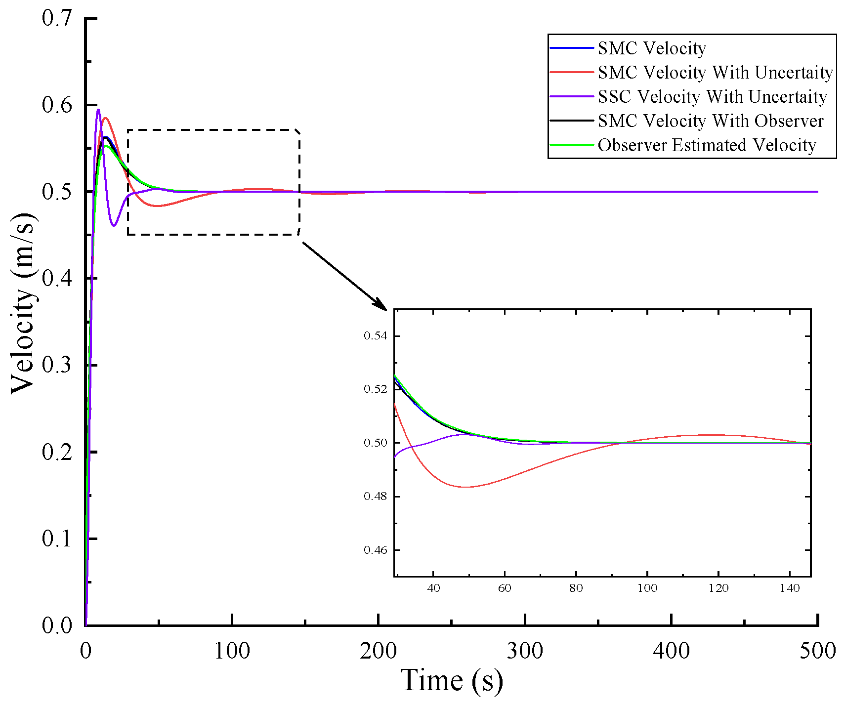
Table 3 shows when there are thruster misalignment and thrust loss, the ${\Phi }_p^u$ value of s-surface speed control is smaller than that of sliding mode control and dual-observer sliding mode control. It proves that the effect of s-surface speed control is better than that of sliding mode control. It can be seen from Figure 8, when there are thruster misalignment and thrust loss, the control effect of velocity control becomes worse, and the overshoot of traditional sliding mode control and s-surface control increases and the stabilization time becomes longer. The overshoot of dual-observer sliding mode controller is small and the stabilization time is short.

As can be seen from

Table 4. The ITAE value comparisons of yaw control.

${\Phi }_p^{\psi }$	SMC with Uncertainty	SSC with Uncertainty	SMC with Observer
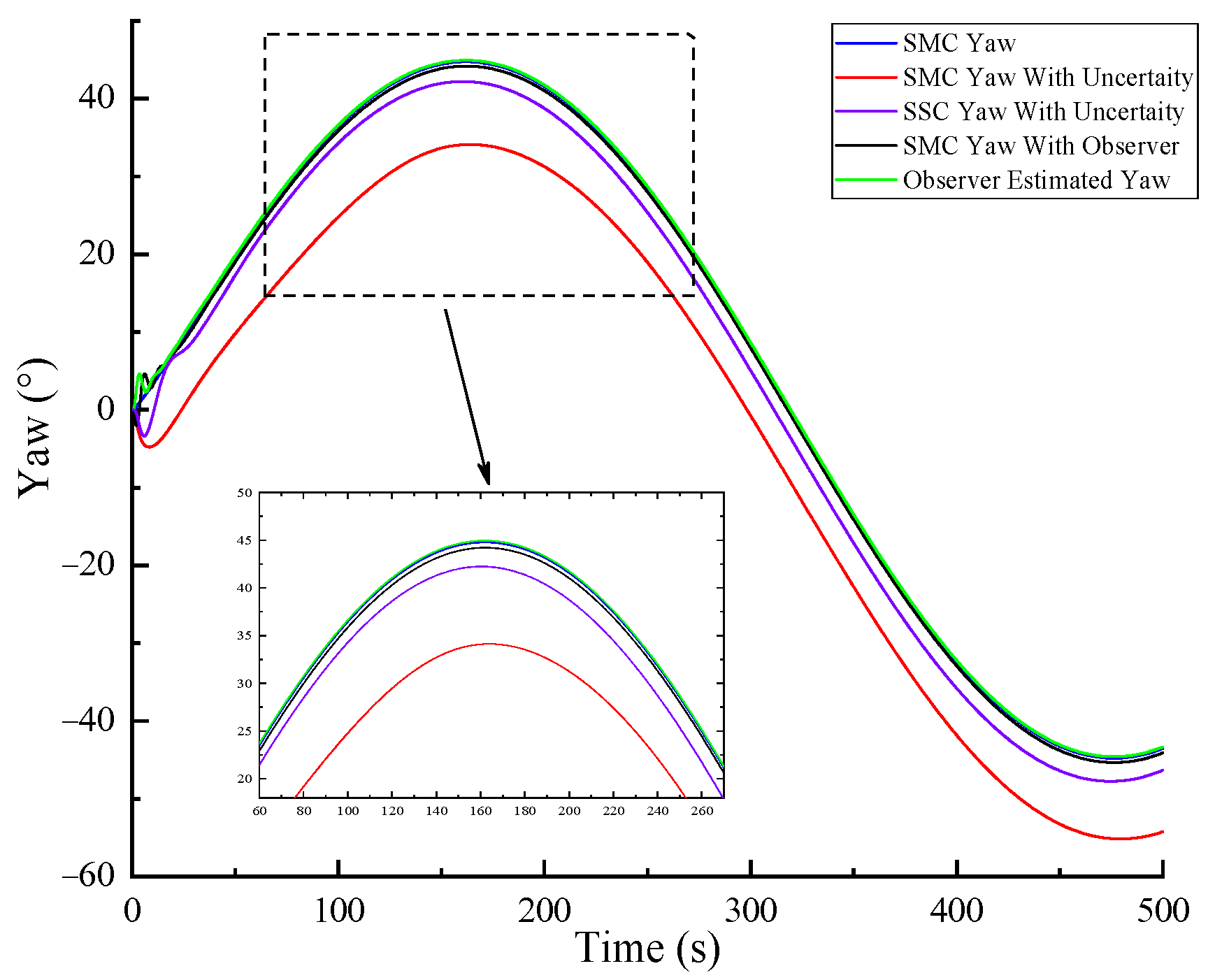
	19230	4542	2976

, when there are thruster misalignment and thrust loss, the ${\Phi }_p^{\psi }$ value of the dual-observer sliding mode control is smaller than that of traditional s-surface and sliding mode control. It can be seen from Figure 9, at this time, there are obvious deviations that cannot be eliminated and the tracking accuracy is decreased. The yaw of dual-observer sliding mode control can track the desired yaw well, which is approximately the same as that without thruster misalignment and thrust loss.

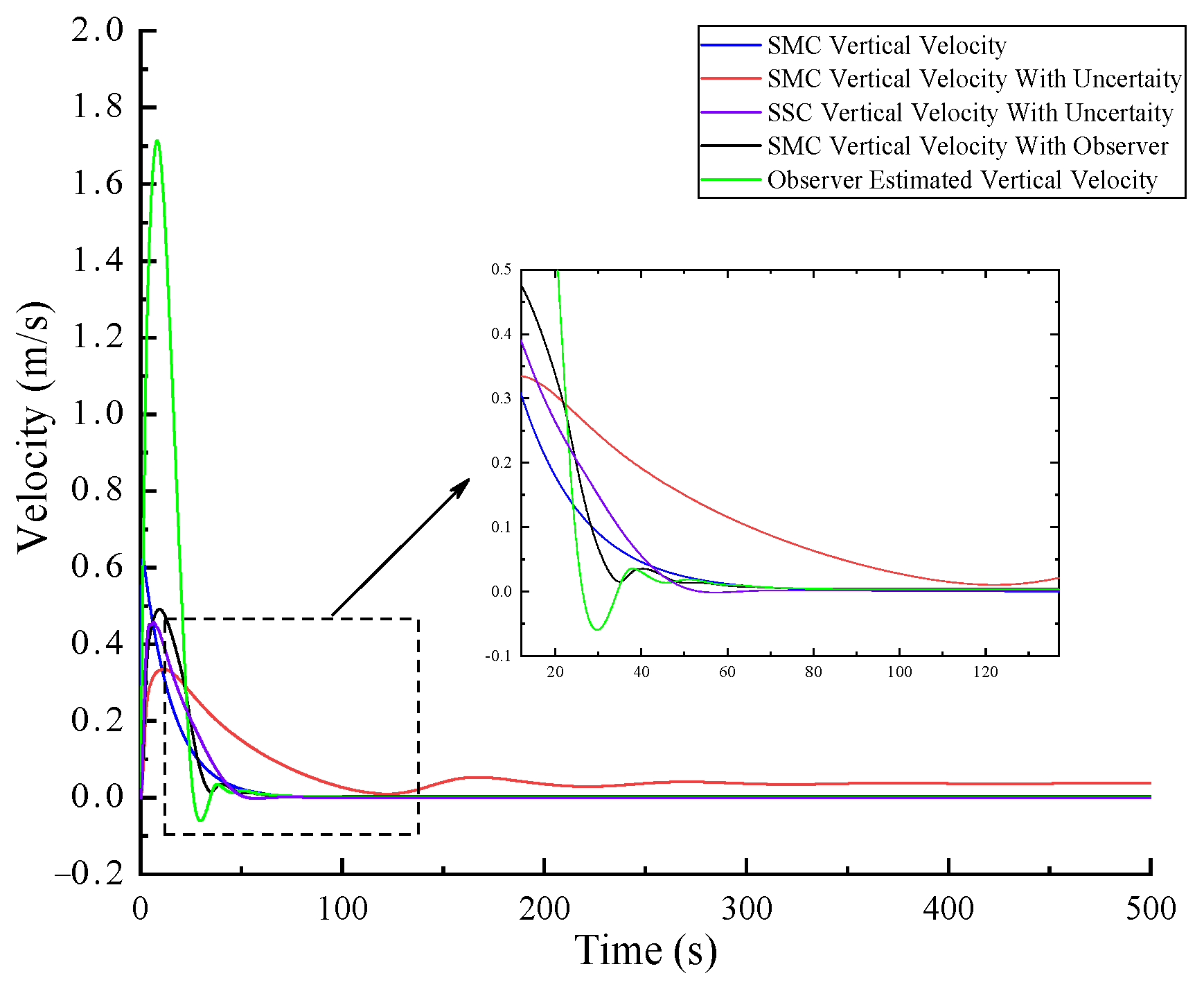
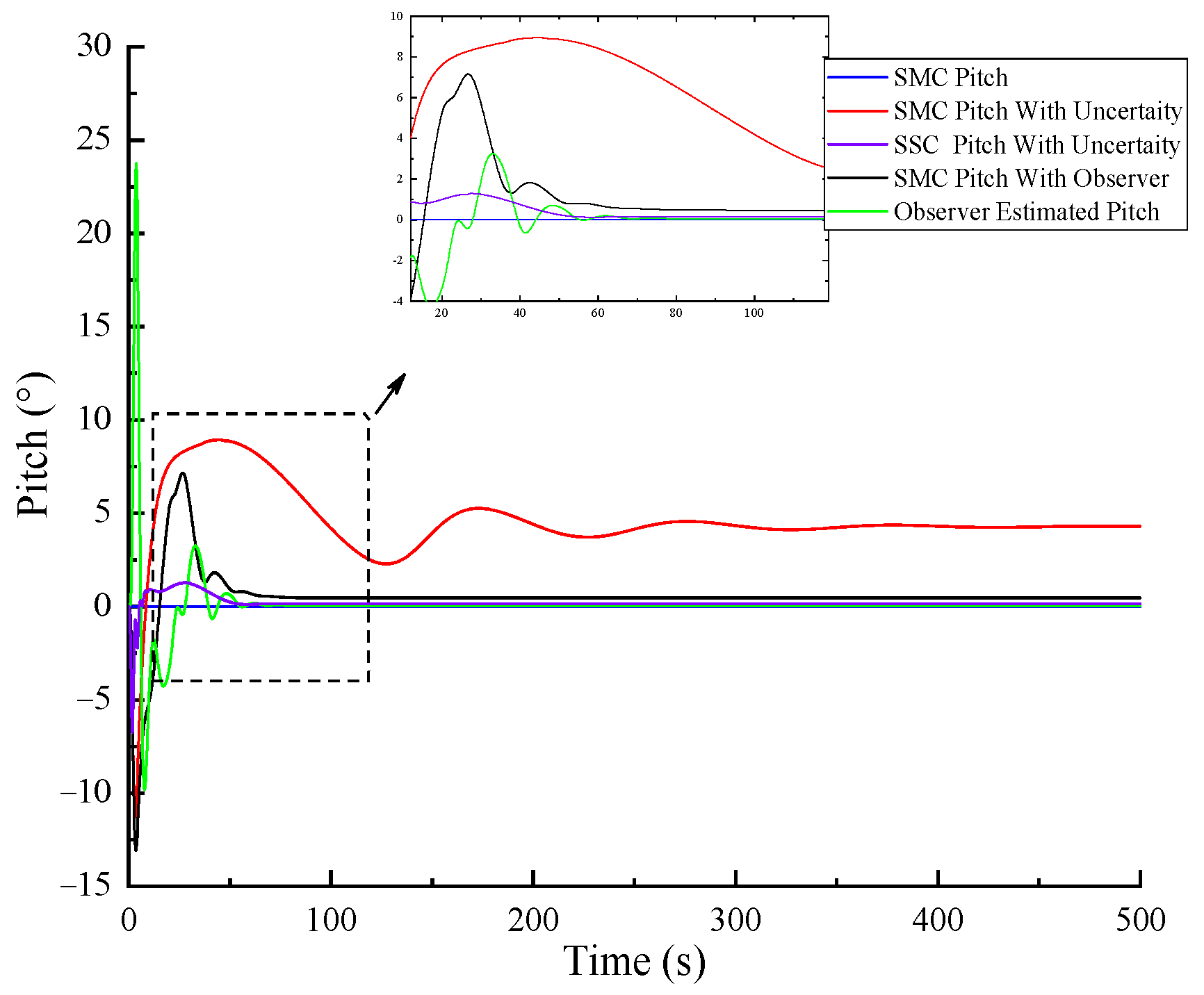
As can be seen from

Table 5. The ITAE value comparisons of pitch control.

${\Phi }_p^{\theta }$	SMC with Uncertainty	SSC with Uncertainty	SMC with Observer
	9474	340	56.35

, when there are thruster misalignment and thrust loss, the ${\Phi }_p^{\theta }$ value of dual-observer sliding mode control is smaller than that of traditional s-surface and sliding mode control. It can be seen from Figure 10 and Figure 11, when there are thruster misalignment and thrust loss, the vertical velocity cannot be zero due to the existence of the pitch. Meanwhile, the pitch changes greatly, and the large stable pitch error is difficult to eliminate. The vertical velocity of the dual-observer sliding mode controller is almost zero and the pitch decreases obviously.

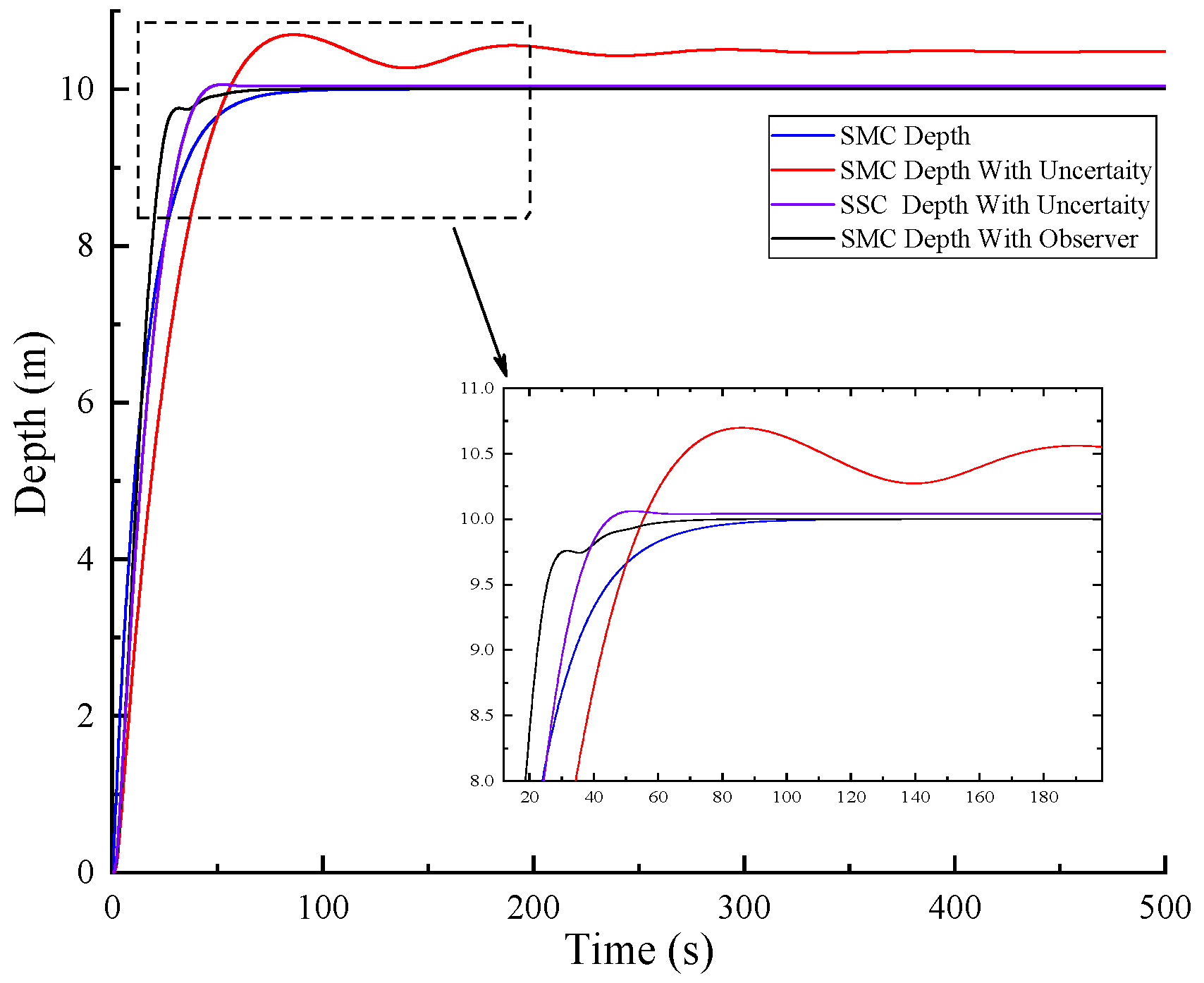
As can be seen from

Table 6. The ITAE value comparisons of depth control.

${\Phi }_p^z$	SMC with Uncertainty	SSC with Uncertainty	SMC with Observer
	62,150	6613	1218

, when there are thruster misalignment and thrust loss, the ${\Phi }_p^z$ value of dual-observer sliding mode control is smaller than that of traditional s-surface and sliding mode control. It can be seen from Figure 12, when there are thruster misalignment and thrust loss, the traditional sliding mode control has a large steady-state error, which is difficult to eliminate, and the response speed of s-surface control is slow. The dual-observer sliding mode controller has a fast response and no steady-state error.

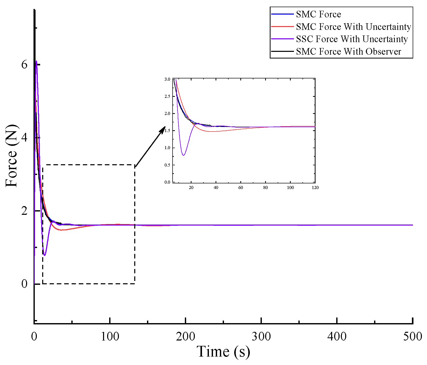
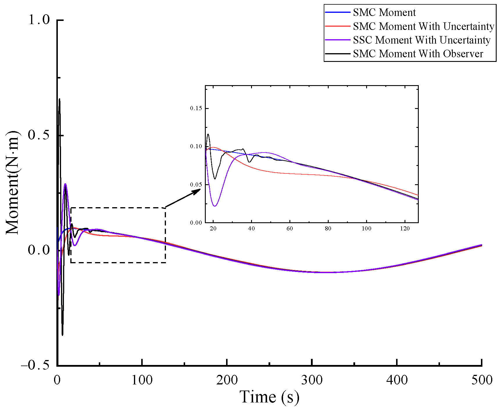
It can be seen from Figure 13, when there are thruster misalignment and thrust loss, the oscillation of the velocity control force in the horizontal plane becomes larger and the stabilization time becomes longer. After the observer compensation, the control force and the expected forward force basically coincide. It can be seen from Figure 14, the deviation of the yaw control moment in the horizontal plane is larger and the stabilization rate slows down. The error between the yaw control moment and the expected moment is small after the estimator compensation. 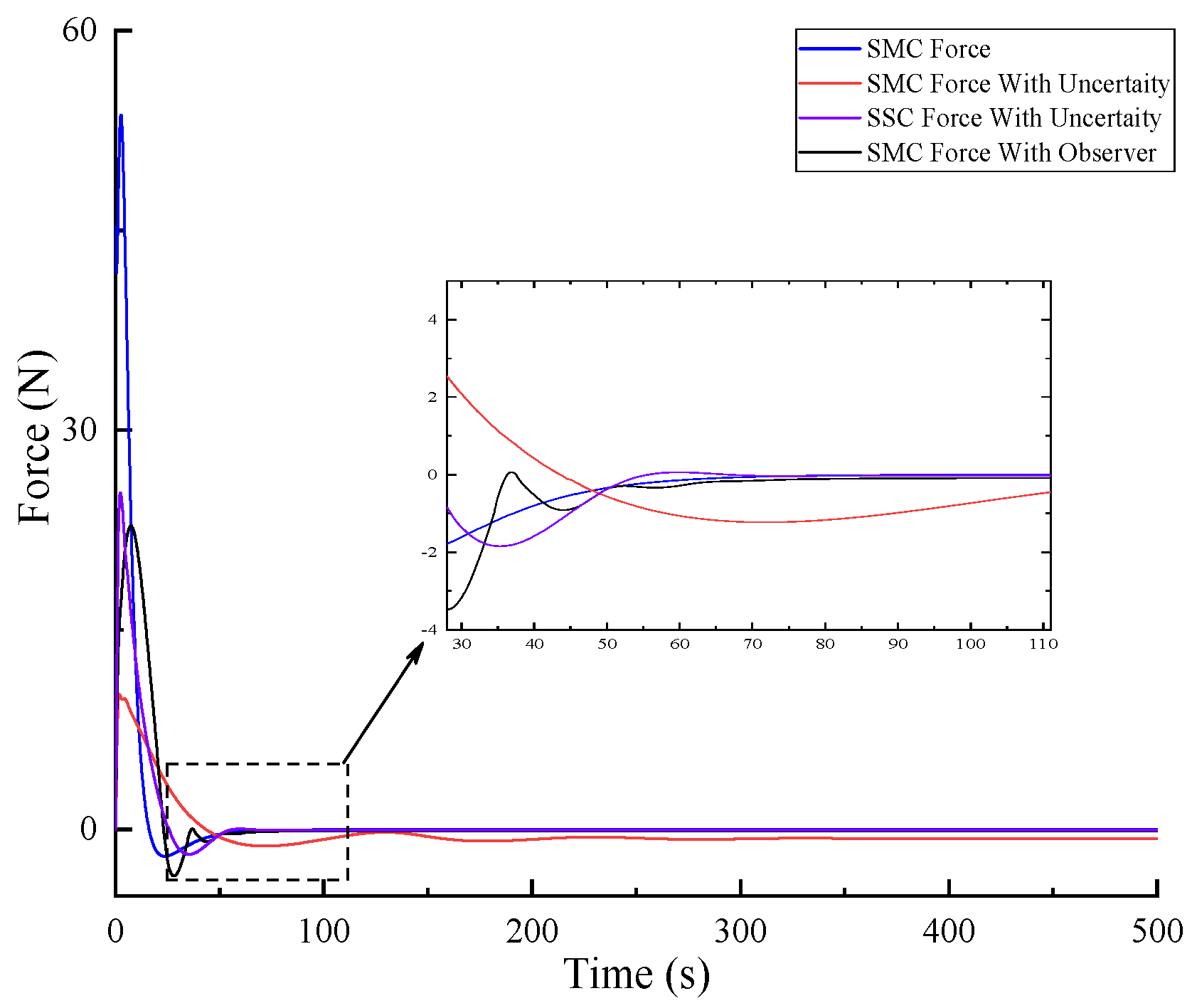It can be seen from Figure 15 that the response time of the vertical force becomes longer in the vertical plane. After stabilization, due to the influence of the pitch, the vertical velocity is not zero. 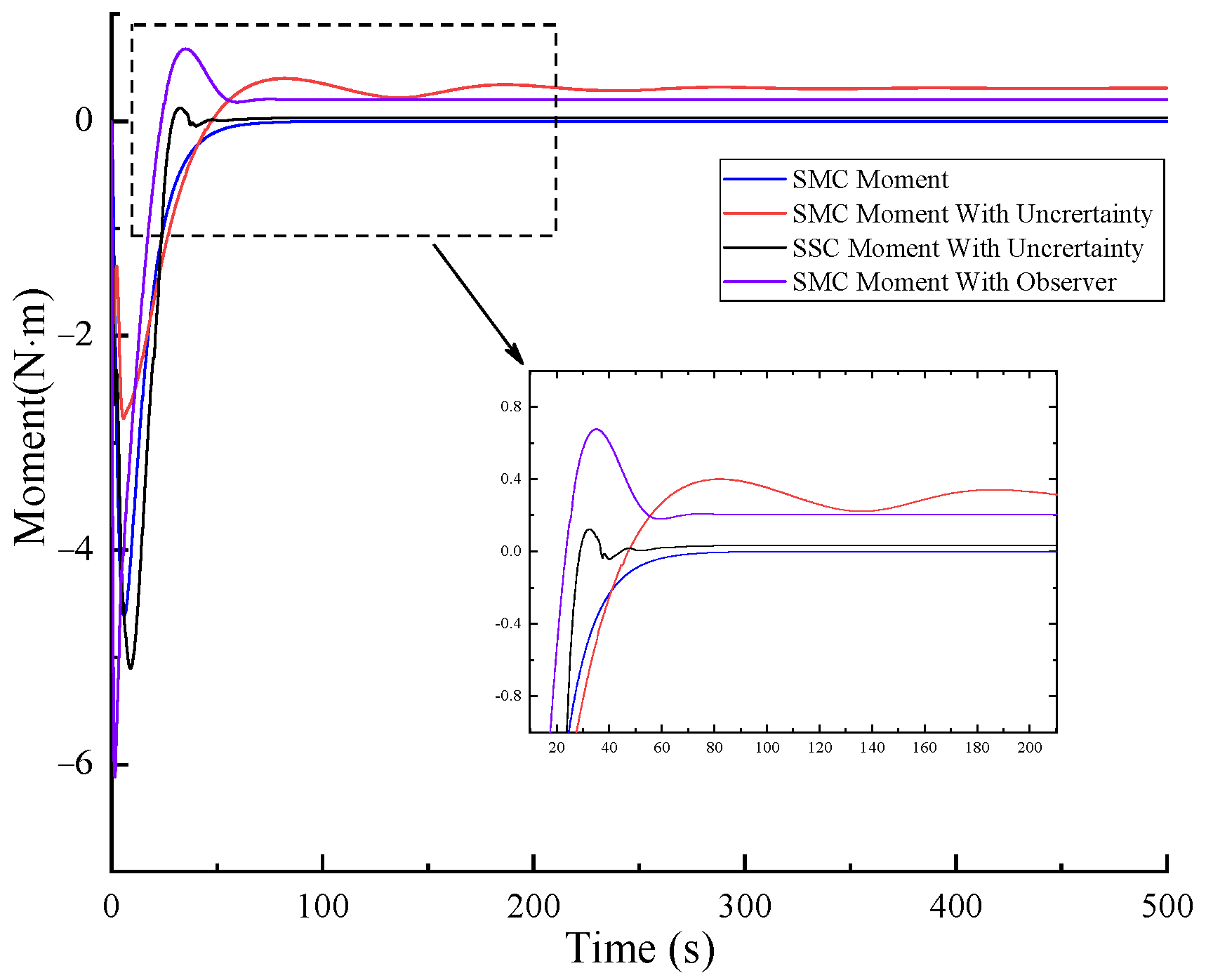It can be seen from Figure 16 that the pitch moment is not zero because there is a stable pitch error, which is difficult to eliminate. After compensation by the observer, the force and moment are basically coincident with the expected force and moment.

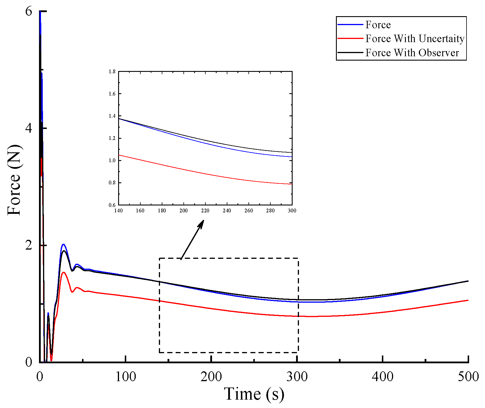
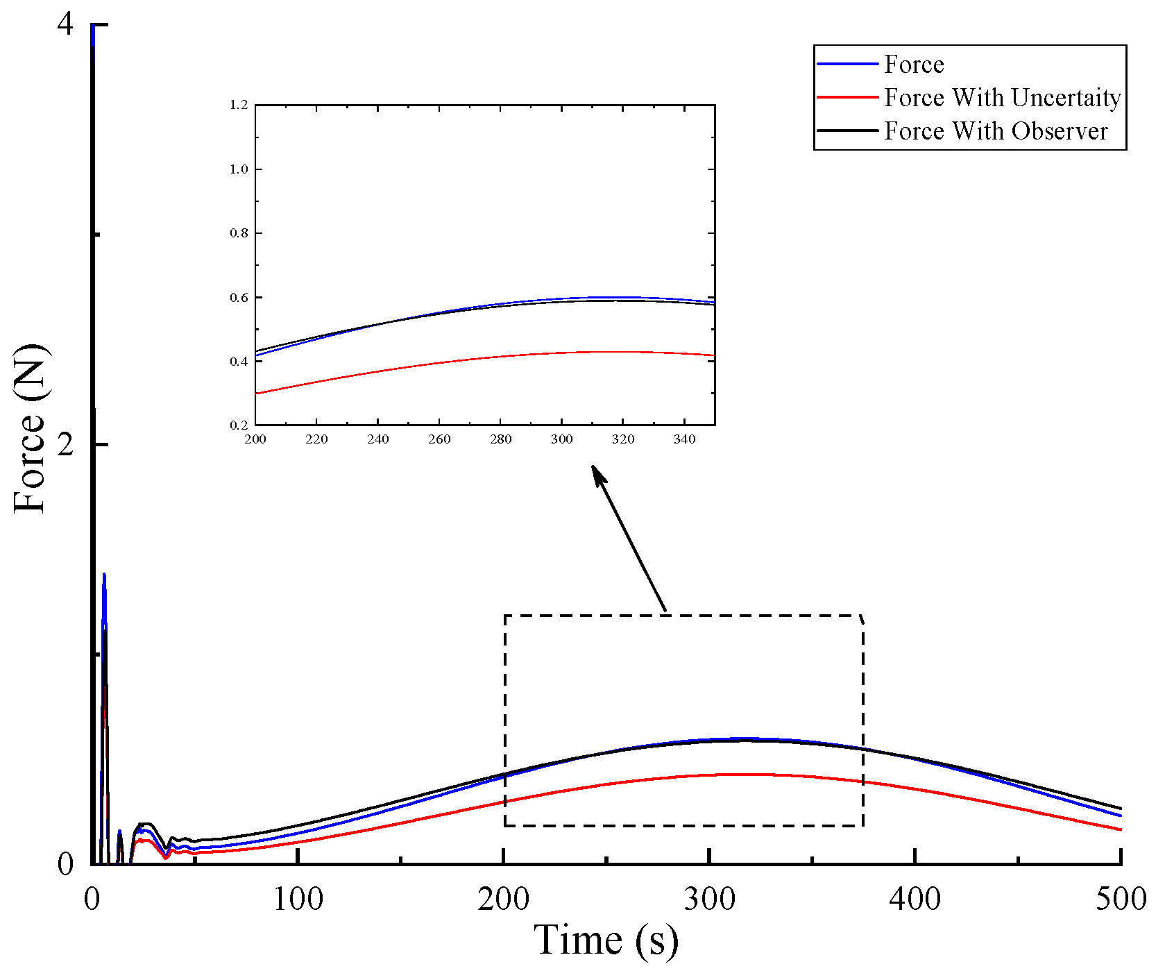
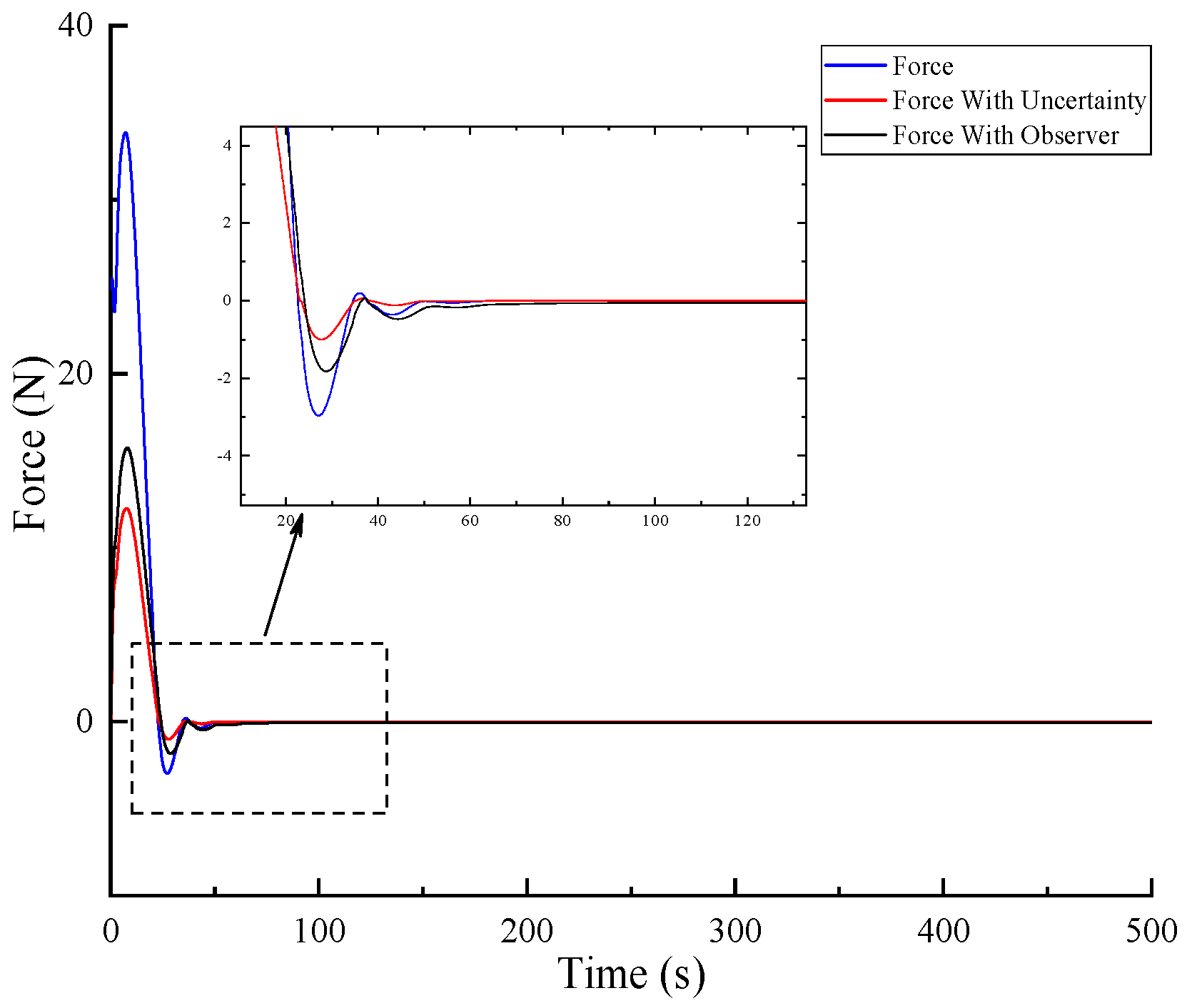
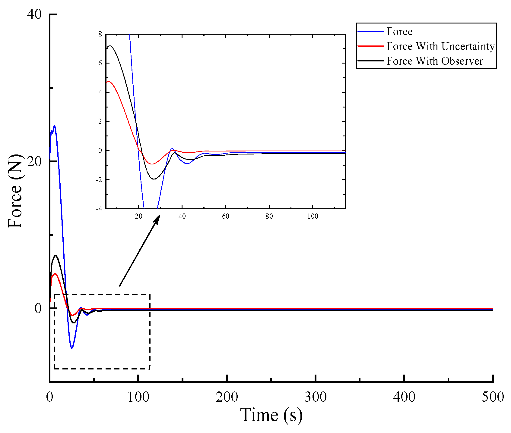
It can be seen from Figure 17 and Figure 18 that, in the presence of thrust loss, the thrust generated by the two thrusters in the horizontal plane is less than the expected thrust value. After compensation by the observer, the thrust is basically equal to the expected thrust. It can be seen from Figure 19 and Figure 20 that the force generated by the two vertical thrusts in the vertical plane is less than the expected thrust value, and, after compensation by the observer, the thrust basically reaches the expected thrust value.

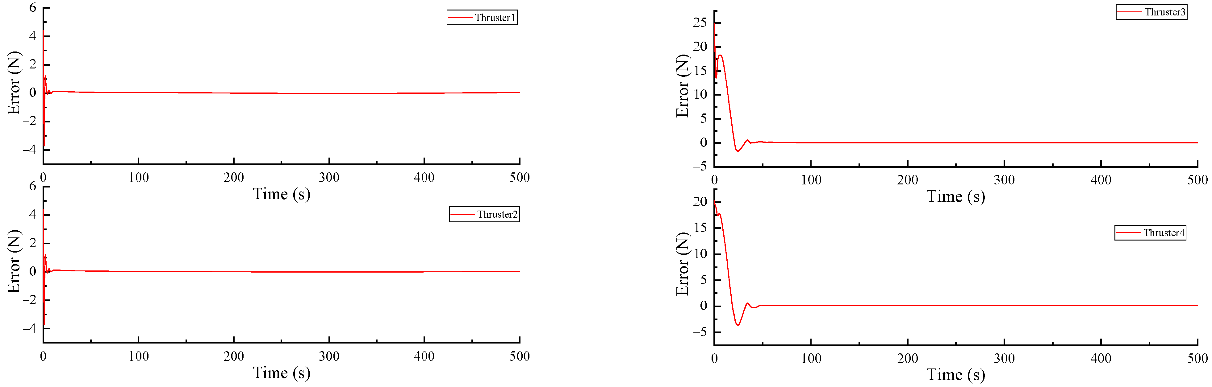
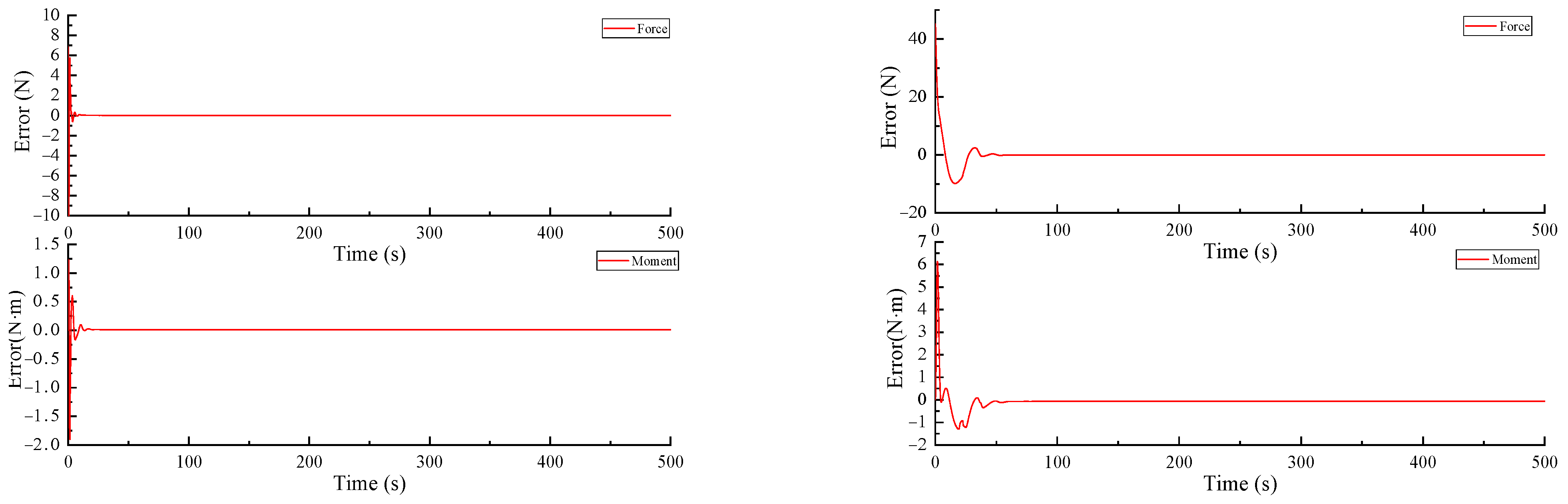
It can be seen from Figure 21 and Figure 22 that the observer error of the thrust loss of the four thrusters converges to zero. The observer errors of the thruster misalignment converge to zero in the horizontal plane and vertical plane.

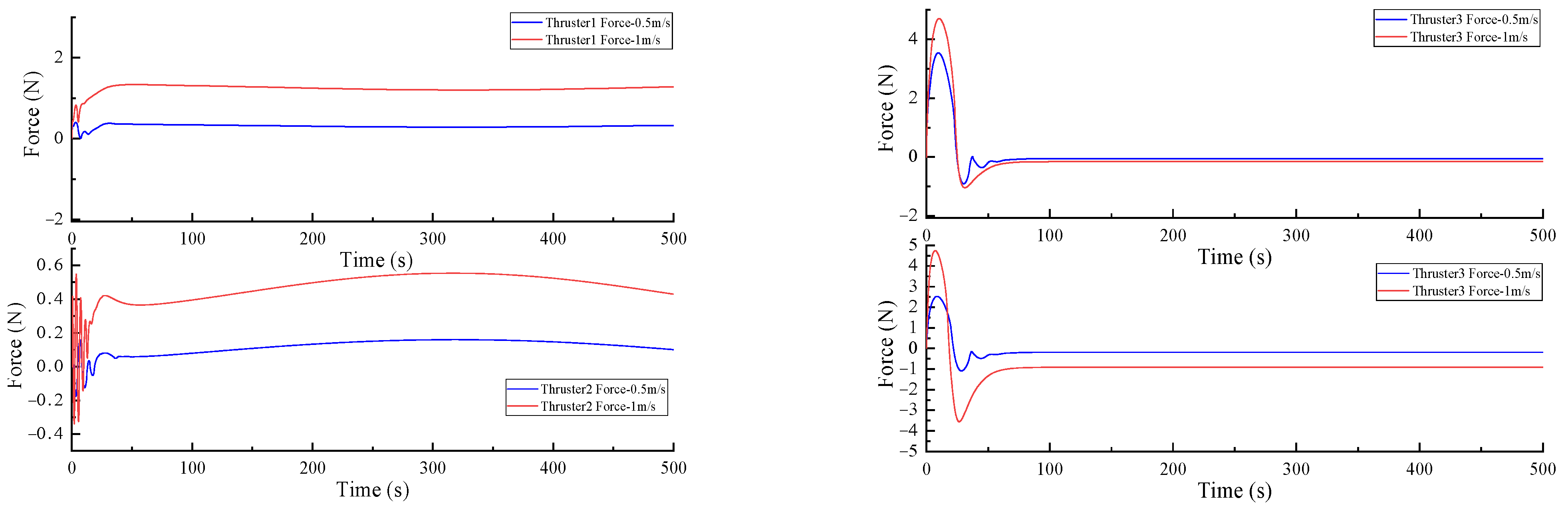
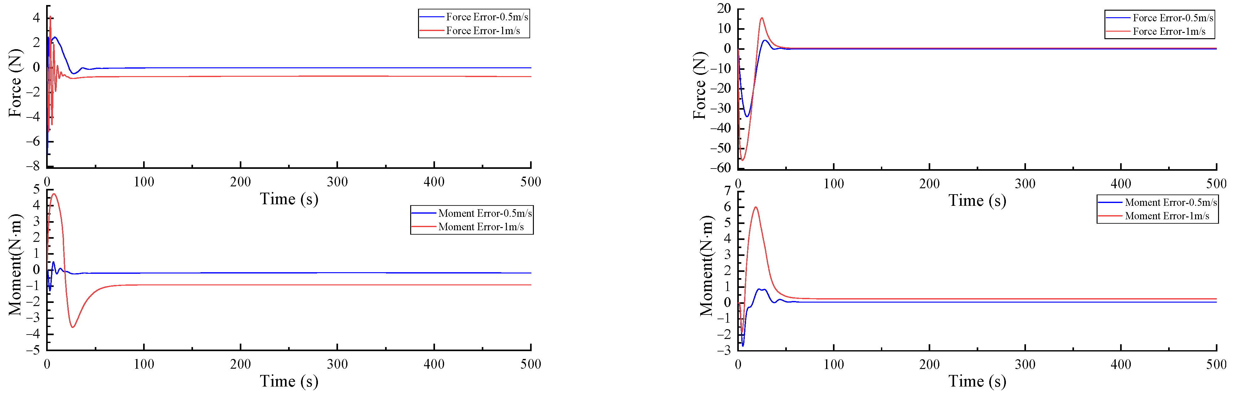
Figure 23 shows that, when the speed increases, the control force also increases and the thrust loss of the four thrusters increases. It can be seen from Figure 24 that, when the speed increases, the errors of force and moment caused by thruster misalignment also increase.

5. Field Test

The field test scene is shown in Figure 25.

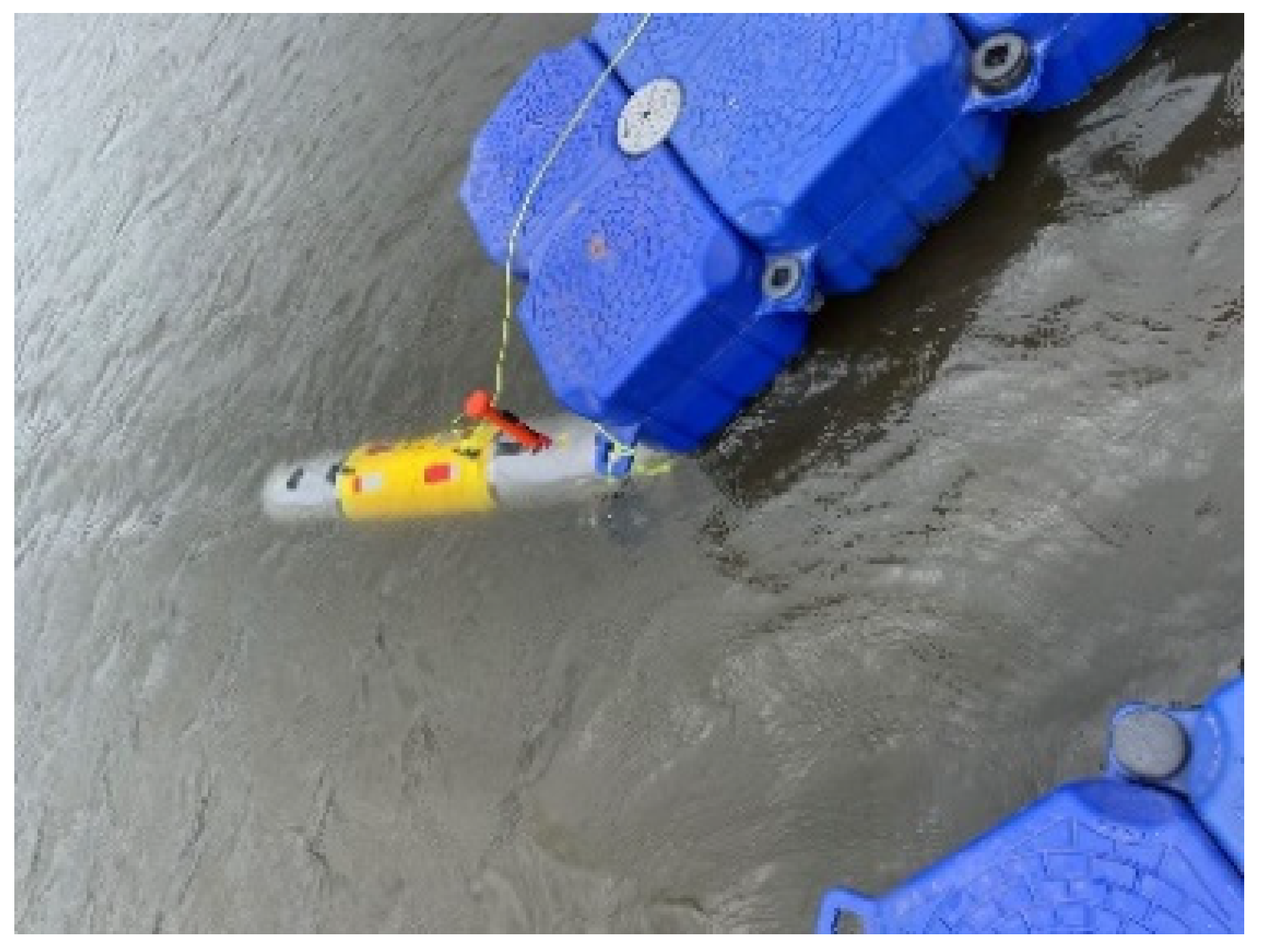
In order to verify the effectiveness of the algorithm, an experiment was carried out in a lake in Harbin in June 2021. The experiments were carried out at 1 m/s and 0.5 m/s, respectively.

Test 1: Set the desired velocity at 1 m/s and the desired yaw at $-{90}^{\circ }\to -{120}^{\circ }\to {40}^{\circ }$. The experimental results obtained are shown from the Figure 26, Figure 27, Figure 28, Figure 29, Figure 30 and Figure 31.

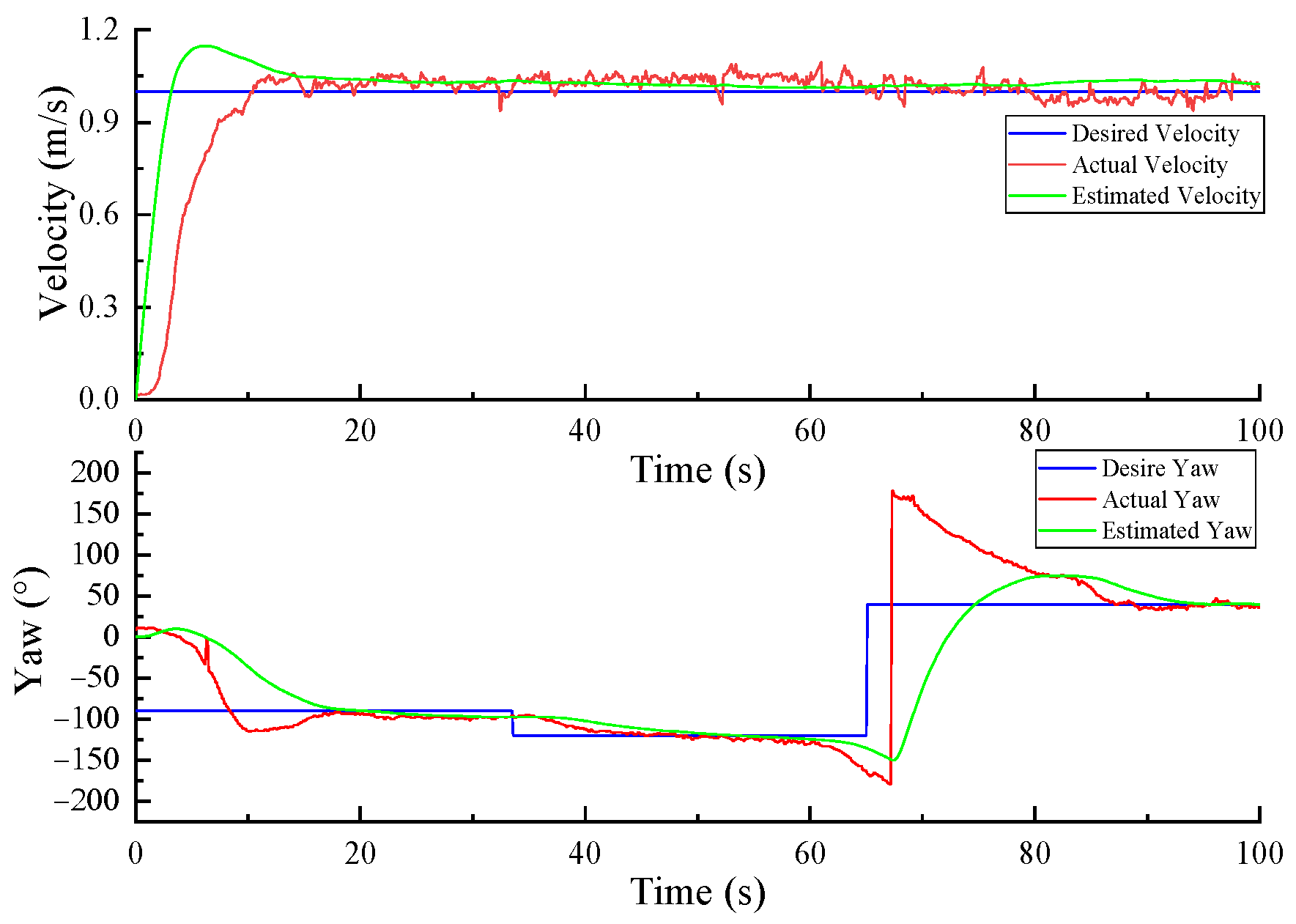
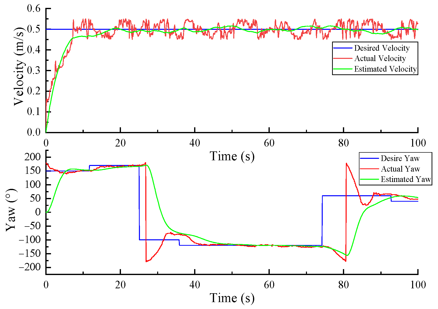
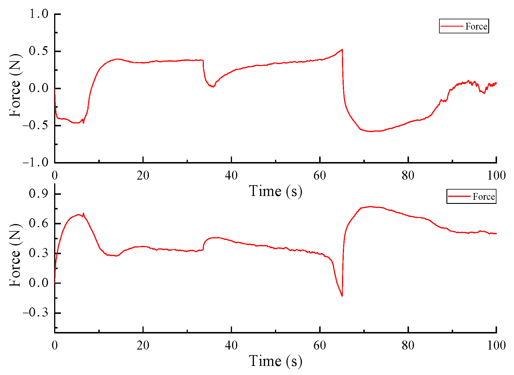
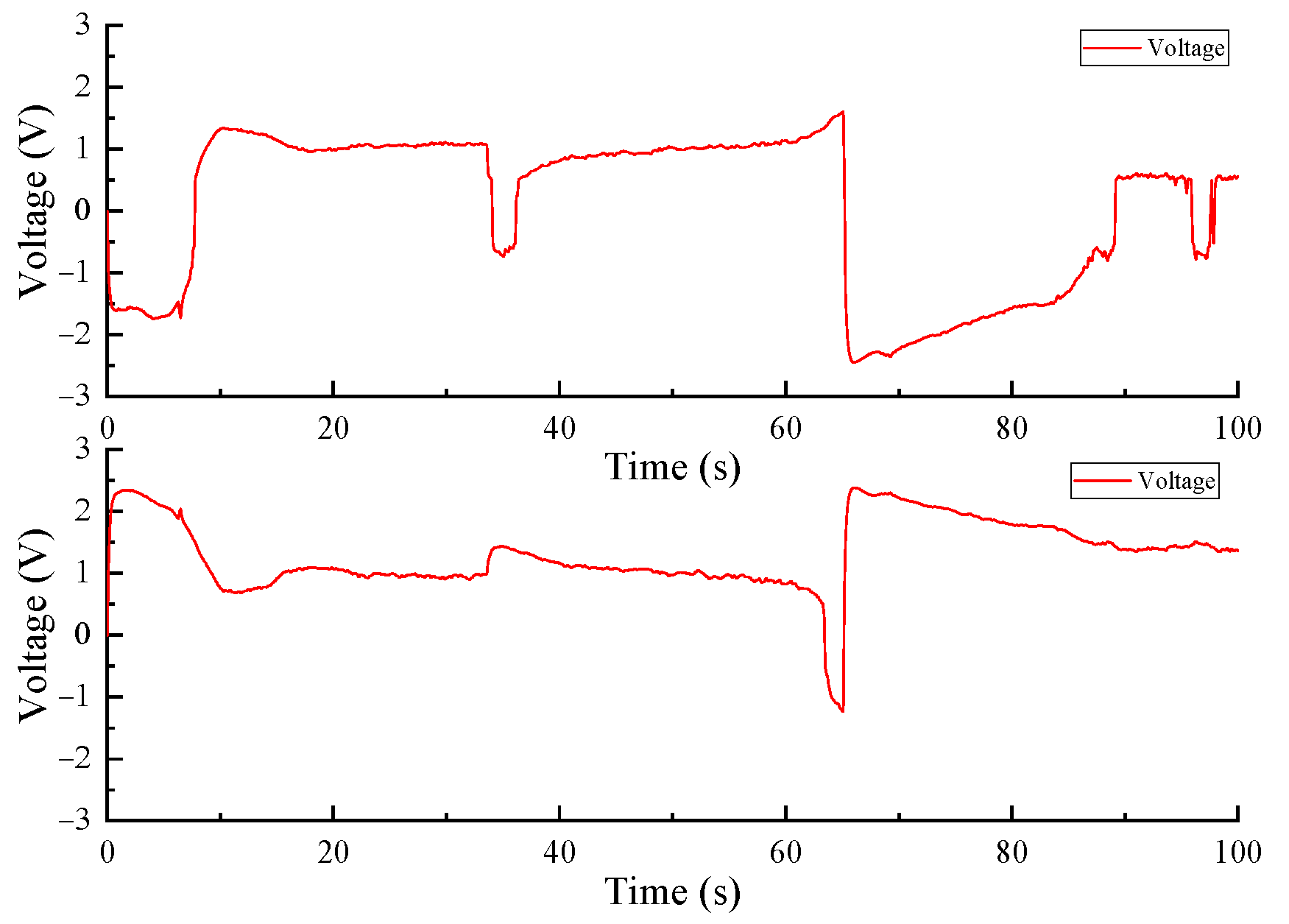
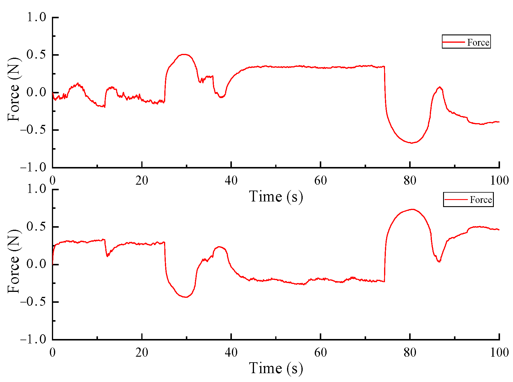
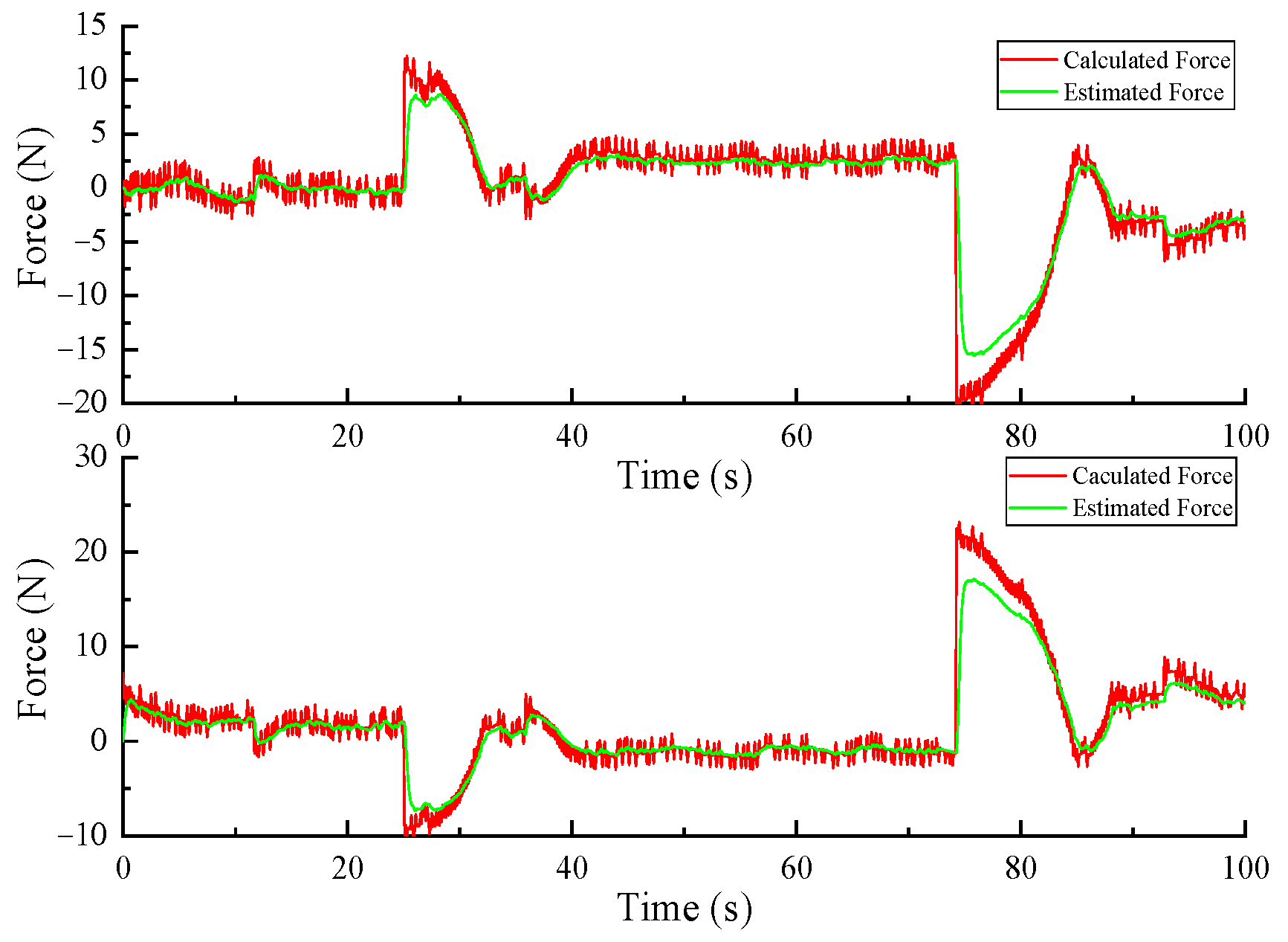
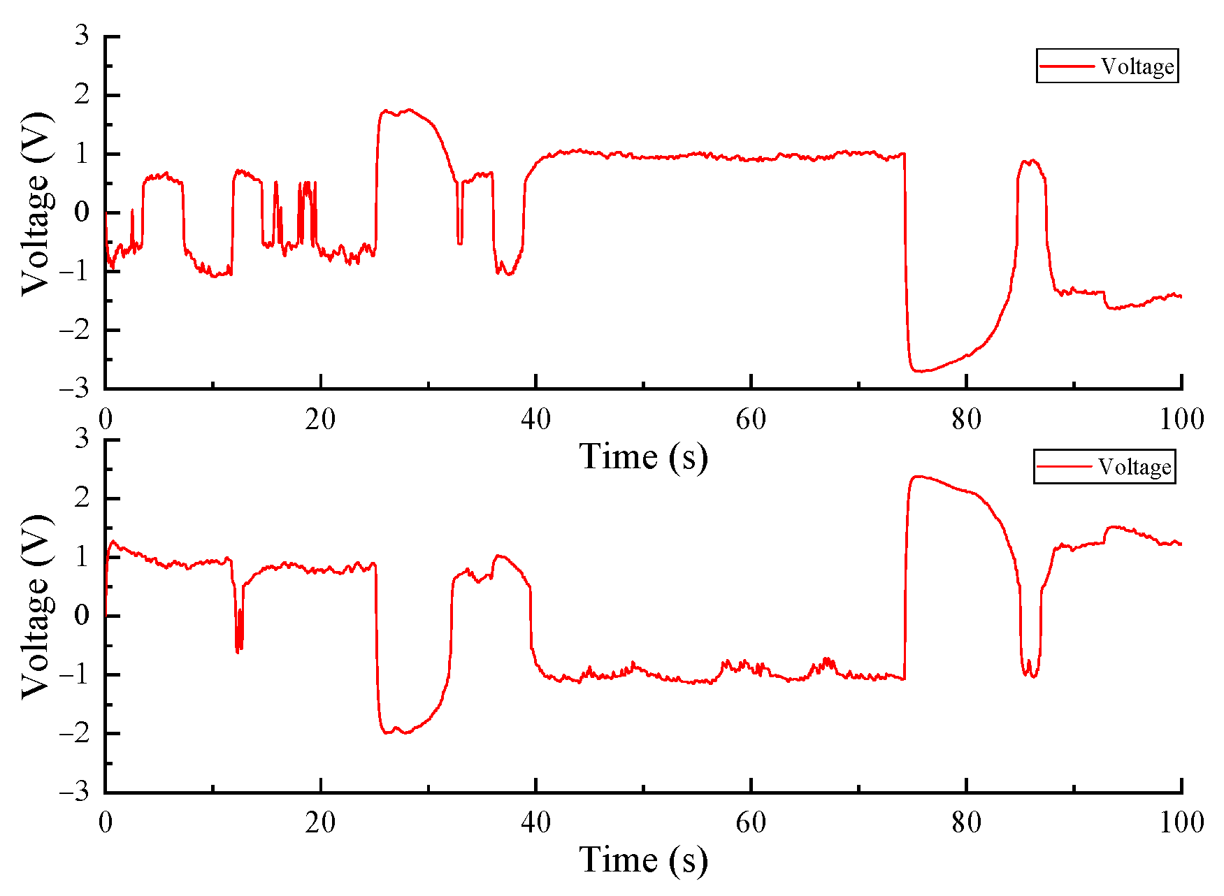
It can be seen from Figure 26 of test 1 that the actual AUV velocity reaches the expected velocity, the AUV velocity estimated by TD disturbance observer is close to the actual velocity obtained by the actual test, the actual yaw reaches the desired yaw, and the yaw estimated by TD disturbance observer is close to the yaw obtained by the actual test. It can be seen from Figure 30 that the calculated output of the thruster is basically consistent with the output estimated by the gain disturbance observer.

Test 2: Set the desired speed at 0.5 m/s and the desired yaw at ${150}^{\circ }\to -{100}^{\circ }\to -{120}^{\circ }\to {50}^{\circ }$. The experimental results obtained are shown from the Figure 32, Figure 33, Figure 34, Figure 35, Figure 36 and Figure 37.

It can be seen from Figure 32 of test 2 that the actual velocity is about the desired velocity, the velocity estimated by TD disturbance observer is close to the actual velocity obtained by the actual test, the actual yaw is close to the desired yaw, and the yaw estimated by TD disturbance observer is close to the yaw obtained by the actual test. It can be seen from Figure 36 that the calculated output of the thruster is basically consistent with the output estimated by the gain disturbance observer.

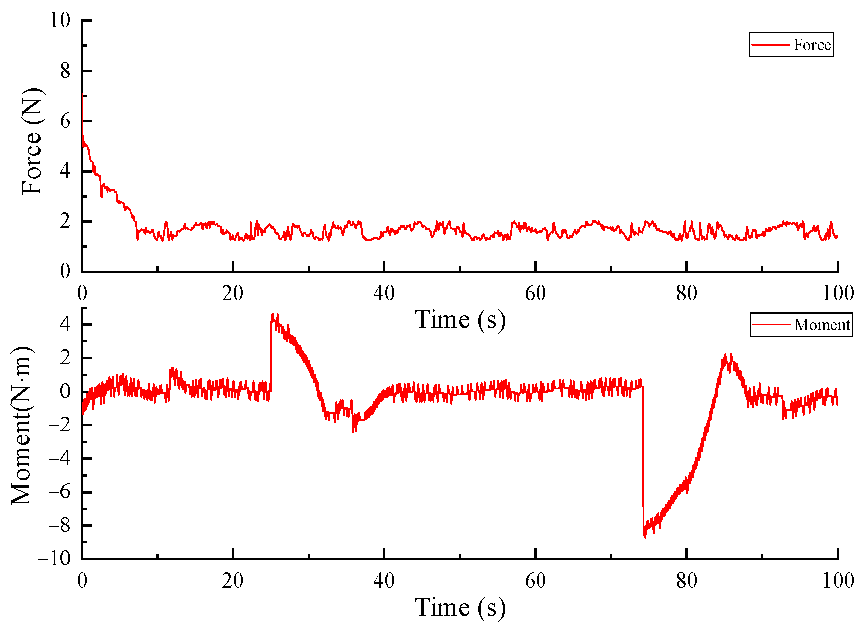
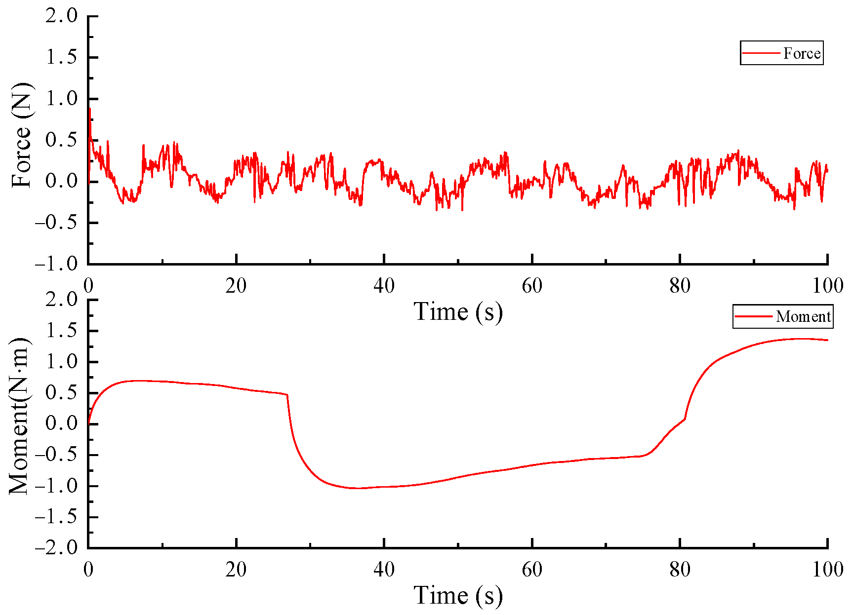
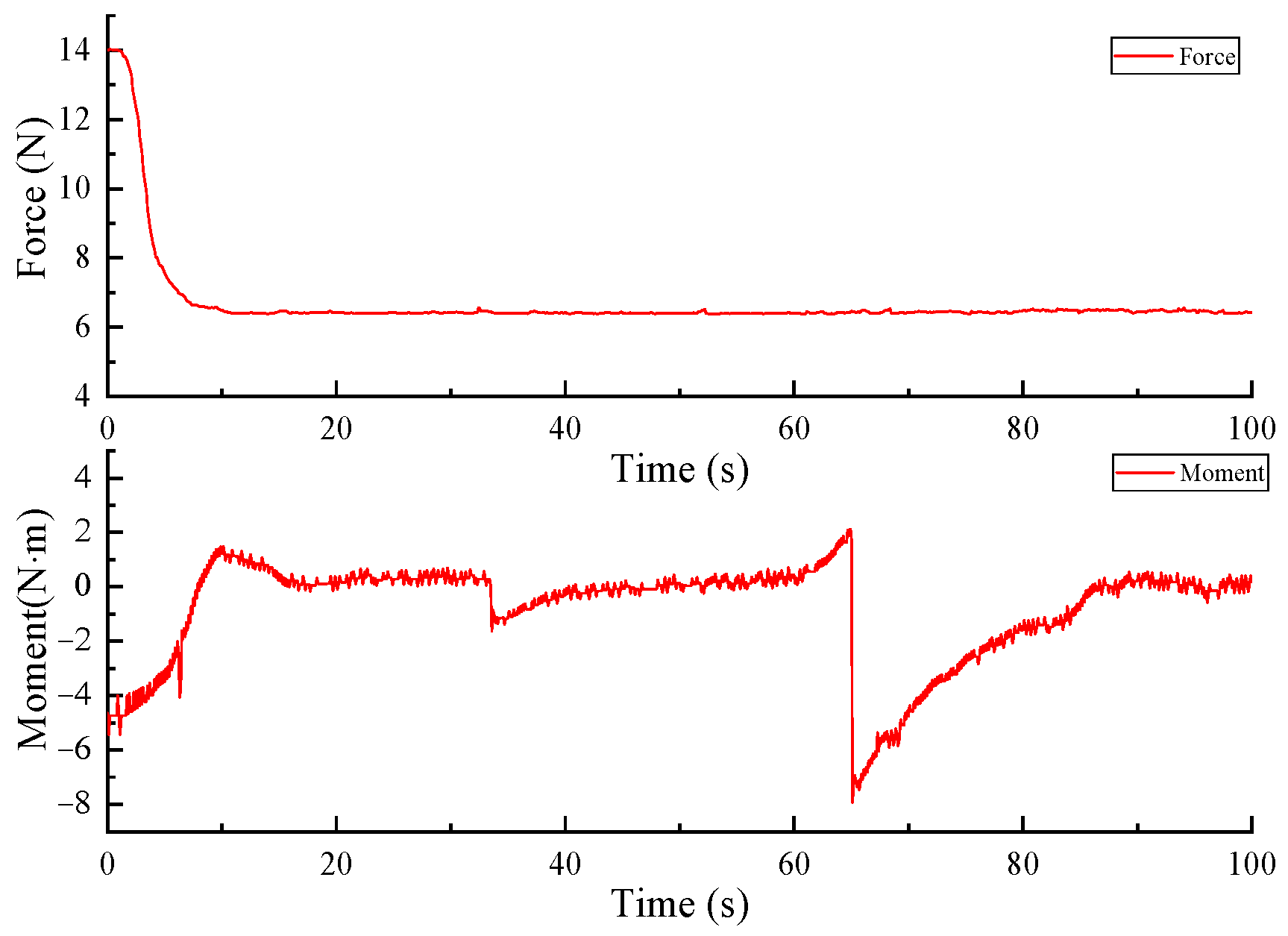
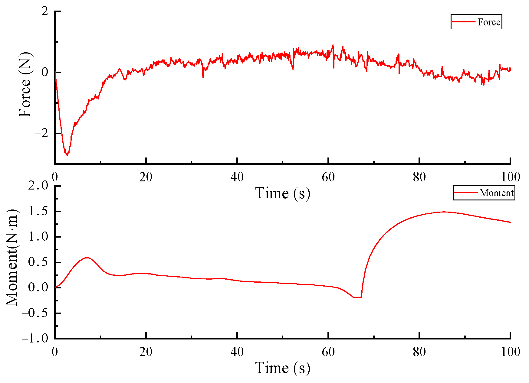
It can be seen from Figure 28 of test 1 and Figure 34 of test 2, when the control force increases, the deviation of force and moment caused by thruster misalignment increases accordingly. According to Figure 31 of test 1 and Figure 37 of test 2, when the control force increases, the thrust loss of the thruster increases correspondingly.

6. Conclusions

This paper addresses the AUV motion control problem in the presence of thruster misalignment and thrust loss by conducting the following studies:

• For the thruster misalignment problem, the deviation of force and torque caused by the thruster installation error is regarded as a nonlinear disturbance that varies with the control force, and a TD disturbance observer is designed for estimation. A sliding mode controller is designed based on the TD disturbance observer to ensure the motion control effect in the presence of thruster installation error, and a Lyapunov function is designed to prove the stability of the system.
• To address the thrust loss problem of the thruster, the thruster dynamics model is introduced and the gain disturbance observer is designed to estimate the thrust loss and the actual output thrust in the presence of thrust loss. When the incoming flow velocity is unknown, the thrust loss is accurately estimated.
• Simulation tests were conducted for AUV motion control in the presence of thruster installation error and thrust loss. The tests proved that the AUV could ensure better control with the compensation of TD interference observer and gain interference observer. At the same time, an external field test was conducted to further verify the effectiveness of the controller.