Prediction-Based Region Tracking Control Scheme for Autonomous Underwater Vehicle

Abstract

This paper addresses the region tracking control problem for an autonomous underwater vehicle (AUV) and proposes a prediction-based region tracking control (PRTC) scheme for AUV. In the PRTC scheme, the idea of prediction is adopted to solve the problems of overshoot and high energy consumption due to the lack of consideration of the large inertia of the AUV in the traditional scheme. The PRTC scheme predicts the future position of AUV through the past time-series position of AUV and the outer boundary of the desired region, and then designs the controller depending on the predicted results. Furthermore, the relationship between the desired region and the control output of the proposed PRTC scheme is studied. It is found that its control output amplitude is susceptible to the desired region range, resulting in output saturation. Therefore, this paper proposes a control law optimization scheme considering the desired region. This optimization scheme modifies the error signal in the control law of the PRTC scheme so that it is only related to the relative position of the desired region where the AUV is located. Finally, the proposed schemes are applied on the ODIN AUV, and the simulation results verify the feasibility of the proposed schemes.

1. Introduction

The autonomous underwater vehicle is currently the only equipment capable of deep-sea work, and it plays an important role in the detection of crashed aircraft and submarine optical cables [1,2]. AUVs that are unmanned and cableless work autonomously in the marine environment. Due to the complex marine environment and the different task requirements of AUVs, the problem of AUV control is one of the current research hotspots in this field [3,4].

AUV control mostly refers to trajectory tracking control, which tracks a predesigned desired trajectory and pursues higher tracking accuracy for the desired trajectory [5,6]. When AUVs perform tasks such as detection of crashed aircraft, the desired trajectory is generally a lawnmower or sawtooth pattern. Performing these tasks, the detection range of the sonar sensor carried by the AUV has overlapping regions. Therefore, in the process of tracking the desired trajectory, there is no need to pursue higher tracking accuracy, but the desired trajectory is changed from a curve to a cylinder with the curve as the centerline, ensuring that the actual trajectory can meet the detection requirements within this cylinder. That is, there is a change from curve tracking to region tracking [7,8,9,10]. The reason to do this is that the pursuit of higher tracking accuracy in curve tracking will cause frequent chattering of the control amount, resulting in increased energy consumption. The region tracking does not pursue higher tracking accuracy, but only requires the actual trajectory to be in the desired region, so as to reduce the frequent chattering of control quantity and reduce energy consumption.

At present, AUV region tracking control is mainly realized based on the scheme of boundary potential energy function. In [7], an AUV region tracking control scheme based on the boundary potential energy function was first proposed. This scheme first constructs a boundary potential energy function, and then integrates the potential energy function into the Lyapunov function, so as to deduce the control law. Reference [8] proposed several approximate Jacobian regions reaching control for robots with uncertain kinematics and dynamics. In this approach, the desired region can be specified as several inequalities. To solve the problem that hydrodynamic parameters of AUV are difficult to obtain accurately, reference [9] proposed a regional tracking control method combining an RBF neural network and boundary potential function. Reference [10] proposed an adaptive region tracking method for an AUV with a redundant thruster system, which carries out the region tracking of AUV in the presence of the thruster fault. Reference [11] addressed the region tracking control problem for AUV with control input saturation, and proposed an adaptive region tracking control scheme based on nonlinear error transformation and prescribed performance control. In [12], the problem of region tracking control based on region constraints was studied. Combined with the techniques of boundary potential energy function and dynamic surface, an adaptive region tracking controller was designed. In [13], an adaptive region tracking control scheme with prescribed transient performance for an AUV with thruster fault was proposed, which can ensure that the tracking error is guaranteed to remain within the prescribed tracking performance.

Further research shows that there is a problem of overshoot in the AUV tracking of the desired region utilizing the above literature schemes, that is, the actual trajectory of the AUV will often exceed the outer boundary of the desired region. To solve this problem, reference [14] designed a control compensation term based on the target speed. This scheme can reduce the number of overshoots to a certain extent, but it still cannot eliminate the overshoot. Reference [15] deduced the control law by constructing a continuous and differentiable piecewise Lyapunov function instead of the boundary potential energy function, and then realized the region tracking through the compensation control scheme. This scheme relies on artificially reducing the outer boundary of the desired region in the controller to realize that the actual trajectory does not exceed the preset outer boundary of the desired region. The function of the outer boundary of the desired region is not fully exerted, which makes the scheme energy-intensive.

Based on the above analysis, aiming at the overshoot problem and high energy consumption of the previous AUV region tracking control schemes, this paper proposes a prediction-based region tracking control (PRTC) scheme for AUV. This scheme considers the large inertia characteristics of AUV, predicts the future position of AUV based on the position information of past time series, and compares it with the outer boundary of the desired region for predictive control. The digital simulation results, which are based on Odin AUV, show that this scheme can complete no overshoot region tracking control, and has obvious advantages in reducing energy consumption.

Then, based on the PRTC scheme, this paper further studies the relationship between the desired region range (the distance from the outer boundary of the desired region to the centerline) and the control output. It is found that in the process of controlling the movement of AUV from the outer boundary to the centerline, the controller output is determined by the error (the distance from AUV to the centerline). The larger the error, the larger the control output. When the desired region is large and the AUV is close to the outer boundary, far from the centerline, the control output is large, which will lead to control output saturation and increased energy consumption. Aiming at this problem, this paper proposes a control law optimization scheme considering the desired region range. The scheme takes the relative value of the distance between the AUV from the centerline and the desired region range as the error signal, and uses this signal as the input signal of the controller. The digital simulation experiment results based on ODIN AUV show that the control law optimization scheme can achieve non-saturated control output and is not affected by the desired region range. Compared with the PRTC scheme, the control law optimization scheme can further reduce energy consumption. The main contributions of this paper are as follows.

In this paper, A PRTC scheme for AUV is proposed, which can conquer the overshoot problem of the traditional region tracking scheme and has lower energy consumption than the traditional scheme.

A control law optimization scheme considering the range of the desired region is proposed, which improves the ability of the PRTC scheme to resist control output saturation and further reduces consumption.

The remainder of this paper is organized as follows. Section 2 elaborates the proposed prediction-based region tracking control scheme in this paper, and describes the idea of the scheme and its implementation process. Section 3 elaborates the proposed control law optimization, considering the desired region range scheme, and explains the idea and implementation process of this scheme. In Section 4, the schemes proposed in Section 2 and Section 3 are verified by a digital simulation experiment. Finally, conclusions are drawn in Section 5.

2. Prediction-Based Region Tracking Control Scheme

This section analyzes the reasons for the overshoot of the traditional region tracking scheme, explains the idea and implementation process of the PRTC scheme proposed in the paper, completes the design of the controller, and gives the stability proof of the controller. Simulation experiments are carried out to compare and verify the feasibility of the PRTC scheme.

2.1. Analyze the Causes of Overshoot in Traditional Schemes and the Idea of the PRTC Scheme

In order to explain how the PRTC scheme solves the problem of overshoot in the traditional scheme, this section analyzes the causes for the overshoot of the traditional scheme and expounds the idea of the PRTC scheme to solve this problem.

2.1.1. Analyze the Causes for the Overshoot of the Traditional Scheme

The traditional scheme [7,8,9,10,11,12] is to derive the control law by incorporating the boundary potential energy function into the Lyapunov function or directly constructing the piecewise Lyapunov function. When the AUV position does not exceed the outer boundary of the desired region, the Lyapunov function value is 0, and the controller does not adjust the AUV position at this time. Once the position of the AUV exceeds the outer boundary of the desired region, the Lyapunov function value is positive, and the controller adjusts the position of the AUV to make it move to the desired region. Based on the above control logic, it can be known that when the controller starts, the actual position of the AUV exceeds the outer boundary of the expected region, and overshoot occurs. At the same time, due to the large inertia of the AUV, the overshoot will continue for a period of time. It is concluded that the fundamental reason for overshoot in traditional schemes is that AUV inertia is not considered, and there is lag in position adjustment.

The root cause of the overshoot in the traditional scheme is that the controller starts to adjust the position when the AUV position exceeds the outer boundary of the desired region.

2.1.2. The Idea of the PRTC Scheme

The basic idea of the PRTC scheme is that considering the large inertia characteristics of AUV, based on the past time-series position information to predict the subsequent position relationship between the AUV and the outer boundary of the desired region, allows one to carry out predictive control. The specific instructions are as follows.

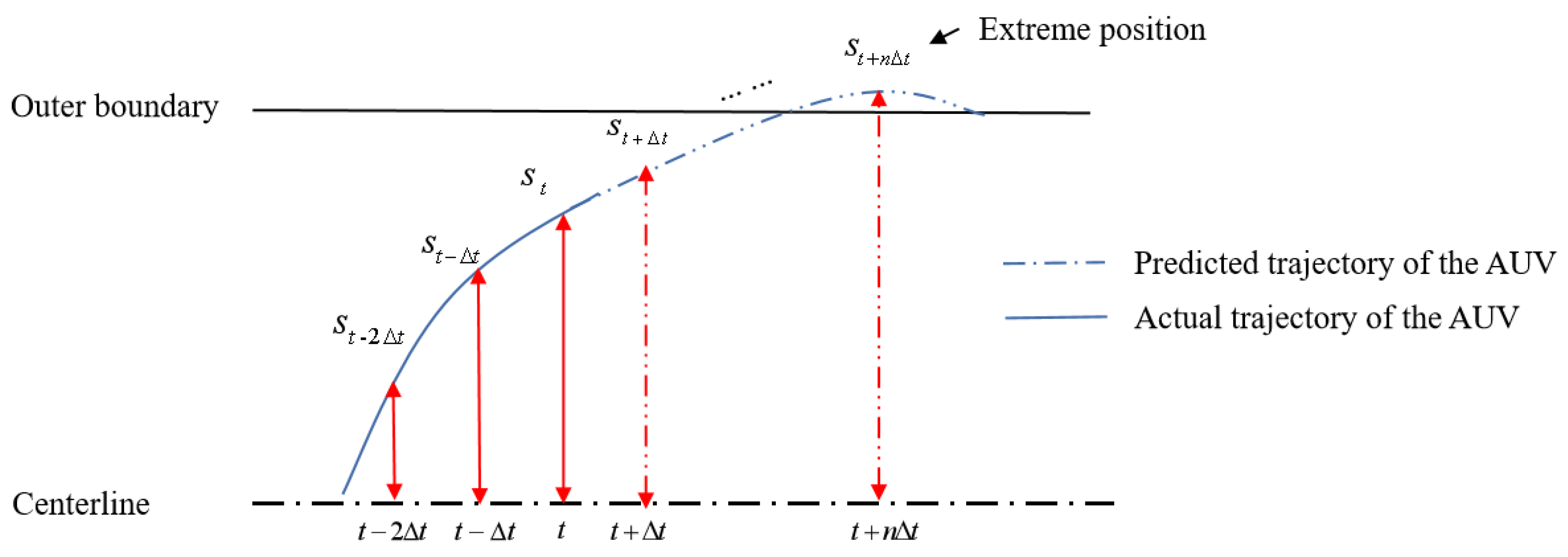
As shown in Figure 1, one must calculate the speed $v_t$ and acceleration $a_t$ of the AUV moving towards the outer boundary of the desired region at time $t$ through the positions $s_{t-2\mathrm{\Delta }t}$, $s_{t-\mathrm{\Delta }t}$, and $s_t$ at time $t-2\mathrm{\Delta }t$, $t-\mathrm{\Delta }t$, and $t$. In this paper, considering the large inertia characteristics of AUV, $v_t$ and $a_t$ at time $t$ are used to calculate the position $s_{t+\mathrm{\Delta }t}$,…,$s_{t+n\mathrm{\Delta }t}$ of the AUV at the subsequent time, so as to realize the prediction of the position of the AUV. When the AUV is in the desired region, the controller is not activated, and no force is given to the AUV in the direction of the centerline of the desired region, so the acceleration of the AUV moving in the direction of the outer boundary is less than zero. Therefore, after several control steps at time $t$, the AUV will move to the extreme position (the point farthest from the desired region center, as shown in Figure 1), and after that, it will be reversed. When it is predicted that this extreme position exceeds the outer boundary of the desired region, the controller starts to pull the AUV toward the centerline of the desired region. In this way, in advance control at time $t$, the extreme position after $t+n\mathrm{\Delta }t$ step will not exceed the outer boundary of the desired region.

According to the above scheme, the AUV can achieve no overshoot region control. However, the position of the AUV will fluctuate near the outer boundary of the desired region, and the random ocean current may cause the AUV to exceed the desired region. For this reason, the controller in the above-mentioned scheme will keep functioning after it is started, so that the AUV moves to the direction of the centerline of the desired region. After AUV returns to the centerline, the controller must be shut down. One must lay a good foundation for the follow-up region tracking.

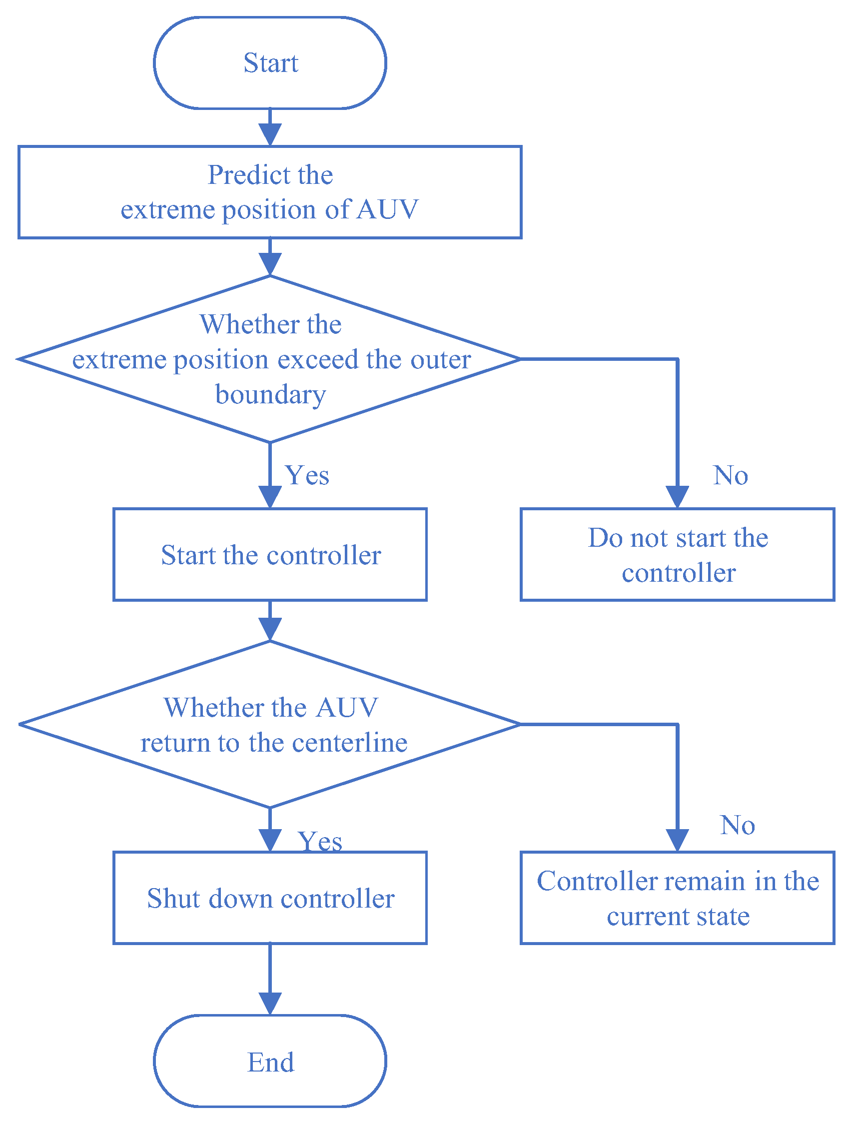
Based on the above idea, the control flow of the PRTC scheme is shown in Figure 2.

Figure 2 shows a complete control flow of the PRTC scheme. The controller has gone through a complete off-on-off process in a control flow. The specific process is as follows: (1)predict the extreme position of AUV; (2) determine whether the extreme position exceeds the outer boundary; (3) determine whether the controller has started based on the judgment result of the first step; (4) after the controller starts, judge whether the limit position extreme position exceeds the centerline; (5) based on the result of the previous step, the controller is shut down or kept in the current state; (6) when the controller is shut down, the control process ends.

2.2. The Implementation Process of the PRTC Scheme

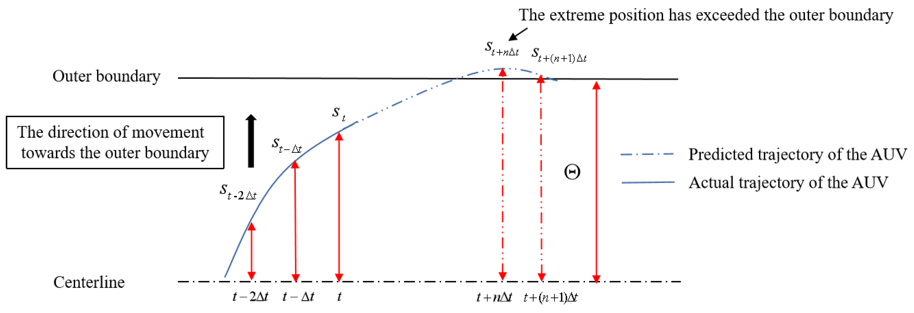
This scheme is implemented in three steps. The relationship of parameters to be used is shown in Figure 3, and the implementation process of each step is described in detail below with reference to Figure 3.

Step 1: Calculate the speed and acceleration of the AUV moving towards the outer boundary of the desired region.

The speed $v_t$ and acceleration $a_t$ of the AUV moving towards the outer boundary of the desired region are obtained by using the distances of the AUV from the outer boundary of the desired region at times $t$, $t-\mathrm{\Delta }t$, and $t-2\mathrm{\Delta }t$ ($\mathrm{\Delta }t$ is the control step). Let the distances of the AUV from the centerline of the desired region at time $t$, $t-\mathrm{\Delta }t$, and $t-2\mathrm{\Delta }t$ be $s_t$, $s_{t-\mathrm{\Delta }t}$, and $s_{t-2\mathrm{\Delta }t}$, respectively. The distance from the outer boundary of the desired region to the centerline is $\mathrm{\Theta }$. Then, the $v_t$ and $a_t$ can be expressed as:

$$\begin{array}{l}{v}_t=\frac{(\mathrm{\Theta }-s_t)-(\mathrm{\Theta }-s_{t-\mathrm{\Delta }t})}{\mathrm{\Delta }t}=\frac{-s_t+s_{t-\mathrm{\Delta }t}}{\mathrm{\Delta }t}\\ v_{t-\mathrm{\Delta }t}=\frac{(\mathrm{\Theta }-s_{t-\mathrm{\Delta }t})-(\mathrm{\Theta }-s_{t-2\mathrm{\Delta }t})}{\mathrm{\Delta }t}=\frac{-s_{t-\mathrm{\Delta }t}+s_{t-2\mathrm{\Delta }t}}{\mathrm{\Delta }t}\end{array}$$

(1)

$$a_t=\frac{v_t-v_{t-\mathrm{\Delta }t}}{\mathrm{\Delta }t}=\frac{-s_t+2s_{t-\mathrm{\Delta }t}-s_{t-2\mathrm{\Delta }t}}{\mathrm{\Delta }{t}^2}$$

(2)

Step 2: Predict the extreme position that the AUV can reach after time $t$.

AUV has the characteristic of large inertia. Without additional control, it can be approximated that the movement trend of AUV after time $t$ is the same as that at time $t$, that is, the acceleration after time $t$ is replaced by $a_t$. Therefore, this paper uses Equations (1) and (2) to predict the AUV position after time $t$. Based on the displacement equation, the predicted position of the AUV for each step after time $t$ is:

$$s_{t+m\mathrm{\Delta }t}=s_t+\overline{v}m\mathrm{\Delta }t+\frac{1}{2}\overline{a}{(m\mathrm{\Delta }t)}^2,m=1,\mathrm{\dots },n,\mathrm{\dots }\infty$$

(3)

where the $m$ represents the number of control steps.

When the AUV is in the desired region, the controller is not activated, which means that no force is given to the AUV in the direction of the centerline of the desired region, and the acceleration of the AUV moving in the direction of the outer boundary is less than zero. Therefore, after reaching the extreme position, the AUV will move to the centerline of the desired region, as shown in Figure 1. This extreme position $s_{t+n\mathrm{\Delta }t}$ can be found by:

$$(s_{t+n\mathrm{\Delta }t}-s_{t+(n-1)\mathrm{\Delta }t})\times (s_{t+(n+1)\mathrm{\Delta }t}-s_{t+n\mathrm{\Delta }t})<0$$

(4)

where the $s_{t+(n-1)\mathrm{\Delta }t}$, $s_{t+n\mathrm{\Delta }t}$, $s_{t+n\mathrm{\Delta }t}$$s_{t+n\mathrm{\Delta }t}$ are the distances from the AUV to the centerline of the desired region at $t+(n-1)\mathrm{\Delta }t$, $t+n\mathrm{\Delta }t$, $t+(n+1)\mathrm{\Delta }t$, respectively. It is worth noting that in the above position prediction process based on Equations (3) and (4), parameter $n$ is an intermediate parameter, which does not need to be expressed concretely.

Step 3: Startup and Shutdown of the Controller.

• Startup of the controller.

The controller will start when the extreme position is predicted to exceed the outer boundary. In order to convert the above process into a logical signal, design the startup functions as:

$$L=\left\{\begin{array}{c}1\begin{array}{ccc}& & \end{array}(|s_{t+n\mathrm{\Delta }t}|-\mathrm{\Theta }\ge 0)\\ 0\begin{array}{ccc}& & \end{array}(|s_{t+n\mathrm{\Delta }t}|-\mathrm{\Theta }<0)\end{array}\right.$$

(5)

As shown in Figure 3, if $\left|s_{t+n\mathrm{\Delta }t}\right|-\mathrm{\Theta }\ge 0$, this indicates that the AUV extreme position exceeds the outer boundary of the desired region; then, for $L=1$ in Equation (5), the controller is started. Otherwise, do not operate the controller.

• Shutdown of the controller.

The above controller remains on after startup until the AUV is pulled back to the centerline of the desired region, then the controller is shut down. In this way, the AUV will be in a position with a large range of free movement in any direction in the desired region, thereby improving the ability to resist ocean current disturbance and laying a good foundation for subsequent region tracking.

By comparing $s_{t-\mathrm{\Delta }t}\times s_t$, judge whether AUV has reached the centerline of the desired region. In this paper, the $s$ above the centerline is positive, and below the centerline is negative. Transform the judgement result into a logical signal, and design the shutdown functions as:

$$L=\left\{\begin{array}{c}1\begin{array}{ccc}& & \end{array}(|s_{t+n\mathrm{\Delta }t}|-\mathrm{\Theta }\ge 0)\\ 0\begin{array}{ccc}& & \end{array}(|s_{t+n\mathrm{\Delta }t}|-\mathrm{\Theta }<0)\end{array}\right.$$

(6)

In Equation (6), if $C=1$, the controller is shut down, otherwise, the controller does not operate.

• Comprehensive realization of startup and shutdown of controller.

The overall process of startup and shutdown in the controller is shown in Figure 2. In order to realize the overall process, it is necessary to design the overall work functions based on the controller startup and shutdown functions. The work functions are as follows:

$$T_t=L+\overline{C}{T}_{t-\mathrm{\Delta }t},LC=0$$

(7)

where $T$ is the work functions of the controller in this paper, and $T_t$ and $T_{t-\mathrm{\Delta }t}$ respectively represent the working state of the work functions at time $t$ and time $t-\mathrm{\Delta }t$. The $LC=0$ is a constraint condition, indicating that $L$ and $C$ cannot be 1 at the meantime.

By Equation (7), the principle of the controller’s working functions is explained. If $L=1$, then $T_t=1$, and the controller is started. If $L=0$, there are two cases: in the first case, $C=0$, $T_t$ is the same as $T_{t-\mathrm{\Delta }t}$, which means that the controller continues to use the working state of the previous step. In the second case, $C=1$, then $T_t=0$, and the controller is shut down. It can be seen that the proposed work functions can realize the overall work process as shown in Figure 2.

In the real applications of the PRTC scheme, the first three control steps are only used to calculate the $s_t$, $s_{t-\mathrm{\Delta }t}$, and $s_{t-2\mathrm{\Delta }t}$. Until the fourth step, according to the flow in Figure 2, the PRTC scheme is used for AUV region tracking control.

2.3. Design Controller of PRTC Scheme

This section completes the controller design based on the implementation process of the PRTC scheme described in Section 2.2. Firstly, the dynamic model in this paper is described, and then the design idea and the implementation of the PRTC controller are given.

2.3.1. Dynamic Model

ODIN AUV is a typical AUV. It has an open dynamic model. Many references use this model to verify the effectiveness of the method [13,16]. Therefore, the controller design and simulation in this paper also use the ODIN AUV model. The ODIN AUV dynamic model is expressed as:

$$M_{\eta }\ddot{\eta }+C_{RB\eta }\dot{\eta }+C_{A\eta }\dot{\eta }+D_{\eta }\dot{\eta }+g_{\eta }=J^{-T}\tau$$

(8)

where, $M_{\eta }=J^{-T}M{J}^{-1}$, $C_{RB\eta }=J^{-T}[C_{RB}-M{J}^{-1}\dot{J}]J^{-1}$, $C_{A\eta }=J^{-T}{C}_A{J}^{-1}$, $D_{\eta }=J^{-T}D{J}^{-1}$, $g_{\eta }=J^{-T}g$; the $\eta$ is a vector about AUV’s position and attitude in the earth-fixed frame. $J$ is the transformation matrix; $M$ is the inertia and added mass matrix; $C_{RB}$ and $C_A$ are rigid-body and Coriolis matrixes; $D$ is the hydrodynamic damping matrix; $g$ is a vector of gravity and buoyancy forces and moments; $\tau$ is the force/moment applied to the AUV. The specific values of each parameter in ODIN AUV can be found in [15,16].

2.3.2. Design Idea and the Implementation of Controller of PRTC Scheme

The control law of the traditional region tracking scheme is obtained based on the method of converging the boundary potential energy functions or the piecewise Lyapunov function to 0. This control law cannot adjust the position of the AUVs in the desired region. In addition, the control law aims to converge the AUVs to the outer boundary of the desired region, so it can only realize the process of pulling the AUVs outside the desired region to the boundary of that. Different from the traditional scheme, the PRTC scheme requires the control law to be able to adjust the position of AUV in the desired region, and at the same time requires the control law to be aimed at the convergence of AUV to the centerline. Hence, the controller law of PRTC scheme cannot be obtained by the traditional scheme.

To meet the above requirements, this paper is inspired by the event triggered control scheme [17]. The event trigger control’s output is adjusted non-periodically by discrete trigger conditions. Based on the above discussion, the controller of PRTC adopts the controller working functions obtained in Section 2.2 as the discrete control trigger condition to switch between interrupted control output and continuous control output. So, the control law of the PRTC scheme is expressed as:

$$M_{\eta }\ddot{\eta }+C_{RB\eta }\dot{\eta }+C_{A\eta }\dot{\eta }+D_{\eta }\dot{\eta }+g_{\eta }=J^{-T}\tau$$

(9)

where, the equation in { } is the typical sliding mode control law, and the derivation process of the control law is common; ${\sigma }_1=s_t+{\dot{s}}_t$; $sign$ is the sign function; $k_1$, $k_2$ are the control parameters.

It can be seen from Equation (7), if $T_t=0$, then the control law is $\tau =0$, indicating that the controller has no control output, that is, the controller is shut down; if $T_t=1$, the control is $\tau =J^T[C_{\eta }\dot{\eta }+D_{\eta }\dot{\eta }+g_{\eta }+\frac{M_{\eta }}{k_1}({\ddot{\eta }}_d-{\dot{s}}_t-k_1{\sigma }_1-k_{2}sign({\sigma }_1))]$, representing that the controller has started and the control output has been adjusted to follow typical sliding mode control law.

2.4. Analysis of Controller Stability of PRTC Scheme

To prove that the AUV can converge to the centerline of the desired region based on the control law in Equation (9), controller stability analysis based on Lyapunov theory is required.

Consider the following Lyapunov function as:

$$V_1=\frac{1}{2}{\sigma }_1^T{\sigma }_1$$

(10)

Differentiating both sides of Equation (10) with respect to time, one has:

$${\dot{V}}_1={\sigma }_1^T{\dot{\sigma }}_1$$

(11)

where

$${\dot{\sigma }}_1=s_t+{\epsilon }_1{\dot{s}}_t$$

(12)

where, the ${\epsilon }_1$ is a small positive number.

According to Figure 3 and the definition of the dynamic model, $s_t$ is equivalent to $\eta -{\eta }_d$. Substituting Equations (8) and (12) into Equation (11), one has:

$${\dot{V}}_1={\sigma }_1^T({\dot{s}}_t+k_1\left\{M_{\eta }{}^{-1}[J^{-T}\tau -C_{\eta }\dot{\eta }-D_{\eta }\dot{\eta }-g_{\eta }]-{\ddot{\eta }}_d\right\})$$

(13)

The control law in Equation (7) will present two control states based on the different values of $T_t$. Firstly, one must analyze the situation of $T_t=1$.

Taking $T_t=1$ in Equation (7) and bringing it into Equation (13), one has:

$$\begin{array}{l}{\dot{V}}_1={\sigma }_1^T(-k_1{\sigma }_1-k_{3}sign({\sigma }_1))\\ {{}^{}}^{}{}^{}=-k_1\left|\right|{\sigma }_1{\left|\right|}^2-k_2\left|{\sigma }_1\right|\\ {{}^{}}^{}{}^{}\le 0\end{array}$$

(14)

where, $\left|\right|\stackrel{}{{\displaystyle }}\left|\right|$ represents the Euclidean norm of the vector.

According to the Lyapunov stability theory, the controller can converge ${\sigma }_1$ to 0 from any initial value at $T_t=1$, that is, the AUV can converge to the centerline of the desired region from any position.

For $T_t=0$, the error variable will diverge because the controller does not have any control output. However, based on the relationship between $T_t$ and the outer boundary of the desired region in Section 2.2, it can be seen that $s_t$ is bounded by $\mathrm{\Theta }$. This is due to the actual assumption that the ${\dot{s}}_t$ is bounded, i.e., $\left|{\dot{s}}_t\right|\le \rho \le \infty$ for positive bound $\rho$. So, the divergence of the error variable ${\sigma }_1$ is bounded. As $s_t$ increases, the $T_t$ jumps from 0 to 1, and the divergence of ${\sigma }_1$ in $T_t=0$ stage will be the initial value of $T_t=1$ stage. According to the above, $T_t=0$ stage does not affect the stability of the controller.

The feasibility of the prediction-based AUV region tracking control scheme will be verified in Section 4 by simulation experiments with the traditional scheme based on boundary potential function.

3. Control Law Optimization Scheme Considering Desired Region Range

Based on the PRTC scheme in Section 2, the relationship between the desired region and the control output is further studied. It is found that the control increases with the expanding of the desired region. This causes control output saturation and increased energy consumption, that is, the control output is affected by the desired region range. Based on this question, this section analyzes the causes of this problem in the PRTC scheme, gives the optimization idea, describes the detailed optimization process, and analyzes the stability of the optimized controller.

3.1. Analyze the Cause for the Problem in the PRTC Scheme and Provide the Optimization Idea

To solve the problem that the control output is affected by the desired region existing in the PRTC scheme, this section first describes the causes of the problem, and then explains how to solve it.

3.1.1. Analyze Cause

The control law of the PRTC scheme, as shown in Equation (9), is obtained by combining the controller work function designed in Section 2.2 with the typical sling mode control law. It can be seen from the constitution of the control law that the control output is determined by the error, the distance between AUV and the centerline of the desired region. The control output increases with the increase of the error. So, when a larger desired region range is selected, the AUV will reach a position farther from the center of the desired region. It makes the error larger, so that the control output is larger, leading to saturation of the control output and expansion of the energy consumption.

3.1.2. Optimization Idea

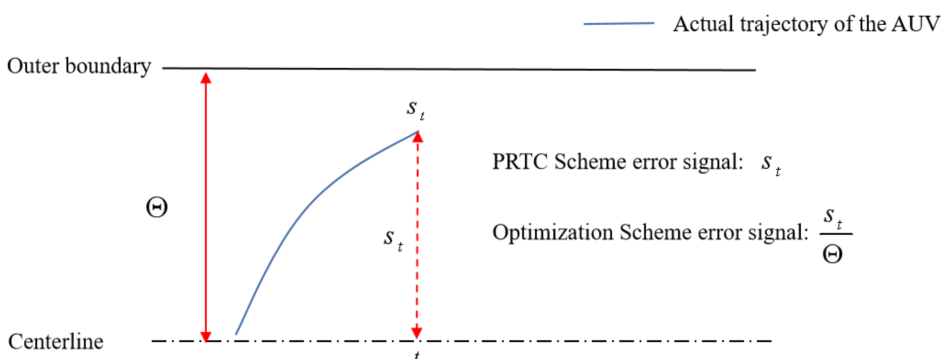
The basic optimization idea is to replace the error signal from the absolute distance between AUV and the centerline of the desired region in the PRTC scheme to the relative distance. The optimization idea is shown in Figure 4.

Replace $s_t$ with $\frac{s_t}{\mathrm{\Theta }}$ as the error signal. It can be seen that when $s_t$ is close to $\mathrm{\Theta }$, $\frac{s_t}{\mathrm{\Theta }}$ is close to 1, and when $s_t$ is close to the center of the desired region, $\frac{s_t}{\mathrm{\Theta }}$ is close to 0. As a result, the error signal fluctuates only in the range of $[0,1)$. Therefore, the optimized control law in this paper will not be affected by the range of the desired region, and can only be adjusted according to the relative position of the AUV in the desired region.

3.2. Describes the Detail of Optimization Process and Analyzes the Stability of the Optimized Controller

Based on the control law optimization idea in Section 3.1, this section describes the detailed optimization process of the control law of the PRTC scheme and analyzes the stability of the optimized controller.

3.2.1. Optimize the Control Law of the PRTC Scheme

The control law optimization scheme is implemented in 2 steps.

Step 1: To eliminate the influence of desired regions on the control law, the error signal $s_t$ in Equation (9) is replaced by $\frac{s_t}{\mathrm{\Theta }}$.

Step 2: To further improve performance and reduce energy consumption, the error signal $\frac{s_t}{\mathrm{\Theta }}$ is nonlinearly transformed as follows:

$${\sigma }_2=sign(s_t+{\epsilon }_1{\dot{s}}_t)\frac{1}{k_3(1-\frac{|s_t+{\epsilon }_1{\dot{s}}_t|}{\mathrm{\Theta }})+\kappa }$$

(15)

where $k_3$, $\kappa$ are positive constants.

Based on steps 1–2, the optimized control law is obtained:

$$\tau =T\left\{J^T[C_{\eta }(\eta ,\dot{\eta })\dot{\eta }+D_{\eta }(\eta ,\dot{\eta })\dot{\eta }+g_{\eta }(\eta )+\frac{M_{\eta }(\eta )}{k_1}({\ddot{\eta }}_d-{\dot{s}}_t-k_1{\sigma }_2-k_{2}sign({\sigma }_2))]\right\}$$

(16)

3.2.2. Stability Analysis

In order to verify that the optimized controller is still stable, a stability analysis is required. Select the Lyapunov function as in Equation (10).

$$V_2=\frac{1}{2}{\sigma }_1^T{\sigma }_1$$

(17)

The derivative of Equation (17) is:

$${\dot{V}}_2={\sigma }_1^T{\dot{\sigma }}_1$$

(18)

Based on Equations (8) and (12), ${\dot{V}}_2$ is further expressed as:

$${\dot{V}}_2={\sigma }_1^T({\dot{s}}_t-{\ddot{\eta }}_d+k_1{M}_{\eta }{}^{-1}(J^{-T}\tau -C_{\eta }\dot{\eta }-D_{\eta }\dot{\eta }-g_{\eta }))$$

(19)

Substitute Equation (16) into Equation (19), which gives:

$${\dot{V}}_2={\sigma }_1^T(-k_1{\sigma }_2-k_{2}sign({\sigma }_2))$$

(20)

According to the error conversion scheme in Section 3.2, the following inequality holds:

$$\frac{1}{k_3(1-\frac{\left|{\epsilon }_1{\dot{s}}_t\right|}{\mathrm{\Theta }})+\kappa }\le \frac{1}{k_3(1-\frac{|s_t+{\epsilon }_1{\dot{s}}_t|}{\mathrm{\Theta }})+\kappa }\le \frac{1}{\kappa }$$

(21)

Using ${\dot{s}}_t$ as bounded based on the above and choosing a small positive ${\epsilon }_1$, $k_3(1-\frac{\left|{\epsilon }_1{\dot{s}}_t\right|}{\mathrm{\Theta }})+\kappa =k_3+\kappa -o>0$ can be guaranteed, where $o$ represents a small positive. It can be seen from Equation (21) that the control law optimization scheme only expands and contracts the error variable ${\sigma }_1$ without changing its sign. Coupling Equation (15), (21) with Equation (20), one has:

$${\dot{V}}_2<{\sigma }_1^T(-\frac{k_1}{k_3+\kappa -o}sign({\sigma }_1)-k_{2}sign({\sigma }_1))\le 0$$

(22)

Based on Lyapunov stability theory, it is proved that the optimized controller remains stable.

4. Simulation Verification

This section verifies the feasibility of the PRTC scheme and control law optimization scheme considering the desired region range. Firstly, the digital simulation setting is given. Then, the comparative results and analysis of the PRTC scheme and boundary potential energy scheme in [15] are given. Finally, the comparative results and analysis of the control law optimization scheme considering the desired region range and the PRTC scheme are given.

4.1. Digital Simulation Settings

Consistent with reference [15], this paper uses Odin AUV as the simulation experiment carrier and 3D elliptical track as the centerline trajectory of the desired region. Among them, the 3D elliptical track affects the three linear motions and three rotary motions, which are mostly used in the reference on AUV control [18]. The rest of the parameters required for the simulation are given below. The parameters of the desired region, the initial state of the AUV, and the saturation limit of the control output are also the same as those in literature [15].

(1)

Centerline trajectory of desired region: a three-dimensional elliptical track, and its specific values are shown in Equations (23) and (24).

$${\eta }_d={[x_d,y_d,z_d,0,0,0]}^T$$

(23)

$$\begin{array}{l}{x}_d=6(1-\cos (0.15t))\\ y_d=3\sin (0.15t)\\ z_d=-0.2x_d\end{array}$$

(24)

where, ${\eta }_d$ is the centerline trajectory of the desired region in this paper; $x_d$, $y_d$, $z_d$ are the trajectories of surge, sway, and heave, respectively; $t$ is the time.

(2)

Desired region: $\mathrm{\Theta }={[0.1,0.1,0.1,0,0,0]}^T$ represents that the distance between the outer boundary of the desired region and the centerline in the direction of surge, sway, and heave is 0.1.

(3)

Initial AUV state: The position and motion state of AUV are set to ${\eta }_0={\dot{\eta }}_0={[0,0,0,0,0,0]}^T$ at the beginning of the simulation.

(4)

Control output maximum limit: ${\tau }_{\max }=[-200,200]$ indicates the maximum range that $\tau$ can take. If $\tau$ exceeds this range, the control output saturation will occur.

(5)

Controller parameters: ${\epsilon }_1={[0.05,0.05,0.05,0.05,0.05,0.05]}^T$$k_1={[1,1,1,1,1,1]}^T$, $k_2={[0.4,0.2,0.2,0.4,0.4,0.4]}^T$, $k_3={[50,50,50,50,50,50]}^T$, $\kappa ={[10,10,10,10,10,10]}^T$; It can be seen from Equation (7) that the value of the controller work function at time $t$ is related to time $t-\mathrm{\Delta }t$. Therefore, the initial state of the working function needs to be set at the beginning. In this paper,$T_0={[0,0,0,0,0,0]}^T$, which means the initial state of the controller is closed. The selection of controller parameters will affect the energy consumption of tracking control. See Section 4.2.3 for relevant analysis.

(6)

Control step and simulation time: The control step is 0.01 s and the simulation time is 50 s, including 5000 control steps.

4.2. Digital Simulation Verification of the PRTC Scheme

This section makes a comparison with the PRTC scheme by adopting the traditional scheme based on the boundary potential energy function [15]. First, to demonstrate that the PRTC scheme can effectively solve the overshoot problem existing in the traditional scheme, the performance of the two schemes in overshoot is analyzed. Then, considering the region tracking scheme to reduce energy consumption as the core, the performance of the two schemes in terms of energy consumption is further analyzed.

4.2.1. Compare the performance of the two schemes in overshoot

Based on the above simulation settings, the tracking errors of the two schemes are shown in Figure 5 and Figure 6.

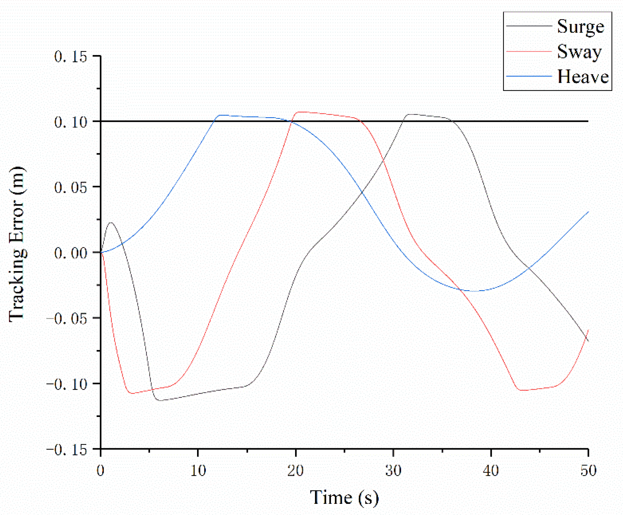
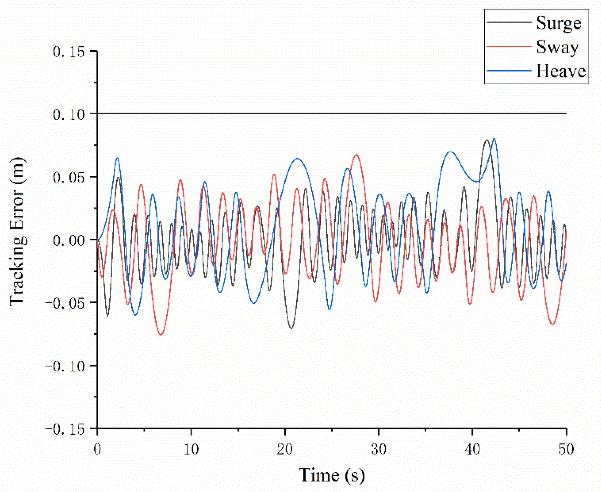
In Figure 5 and Figure 6, the black, red, and blue lines represent the tracking errors in the surge, sway, and heave directions, respectively. The horizontal line parallel to the X axis in the figure represents one side of the outer boundary of the desired region.

It can be seen from Figure 5 and Figure 6 that the tracking error of the traditional scheme often exceeds the outer boundary of the expected region, and there is a long overshoot time. However, the AUV in the PRTC scheme does not exceed the outer boundary of the expected region. As can be seen from Figure 6, in the PRTC scheme, when the AUV is close to the outer boundary of the desired region, it will be pulled back to the center of the desired region, while the traditional scheme does not have this process. The process of AUV returning to the center of the desired region in Figure 5 is caused by the change of the centerline trajectory of the desired region itself.

In order to quantitatively analyze the effect of the proposed scheme and facilitate the comparison, the specific data in Figure 5 and Figure 6 are extracted. The specific data are presented in

Table 1. Performance of PRTC scheme and traditional scheme in overshoot.

Scheme	Overshoot Judgement			Overshoot Time Accounts for the Total (%)			Maximum Overshoot (mm)
	Surge	Sway	Heave	Surge	Sway	Heave	Surge	Sway	Heave
Traditional scheme	Yes	Yes	Yes	29.27	24.82	7.70	+13.16	+8.25	+5.35
PRTC scheme	No	No	No	0	0	0	−14.20	−29.65	−19.75

.

According to Table 1, the traditional scheme has overshoot in the three directions of surge, sway, and heave, and the overshoot time accounts for the total 29.27%, 24.82%, and 7.70%, respectively. The PRTC scheme does not have overshoot, which solves the problem of overshoot in the traditional schemes. From the analysis of maximum overshoot, for the maximum overshoot item in Table 1, the positive sign indicates overshoot, the negative sign indicates no overshoot, and the subsequent number indicates the distance between the extreme position and the outer boundary. The maximum overshoot of the traditional scheme in the three directions of surge, sway, and heave is 13.16 mm, 8.25 mm, and 5.35 mm, respectively. The distance between the extreme position of PRTC scheme and the outer boundary is −14.20 mm, −29.65 mm, and −19.75 mm in three directions, respectively. This shows that the PRTC scheme can make full use of the desired region without overshoot.

4.2.2. Compare the Performance of the Two Schemes in Terms of Energy Consumption

Energy consumption is mostly calculated by Equation (25) [15]:

$$E_j={\displaystyle \sum _{\kappa =1}^N|{\tau }_j(t)|}$$

(25)

In Equation (25), $N$ is the number of control steps, which is obtained by dividing the simulation time by one control step time; ${\tau }_j,j=x,y,z$ represents the controller output in the three directions of surge, sway, and heave, respectively.

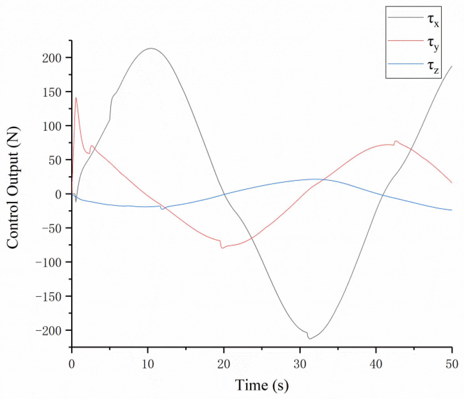
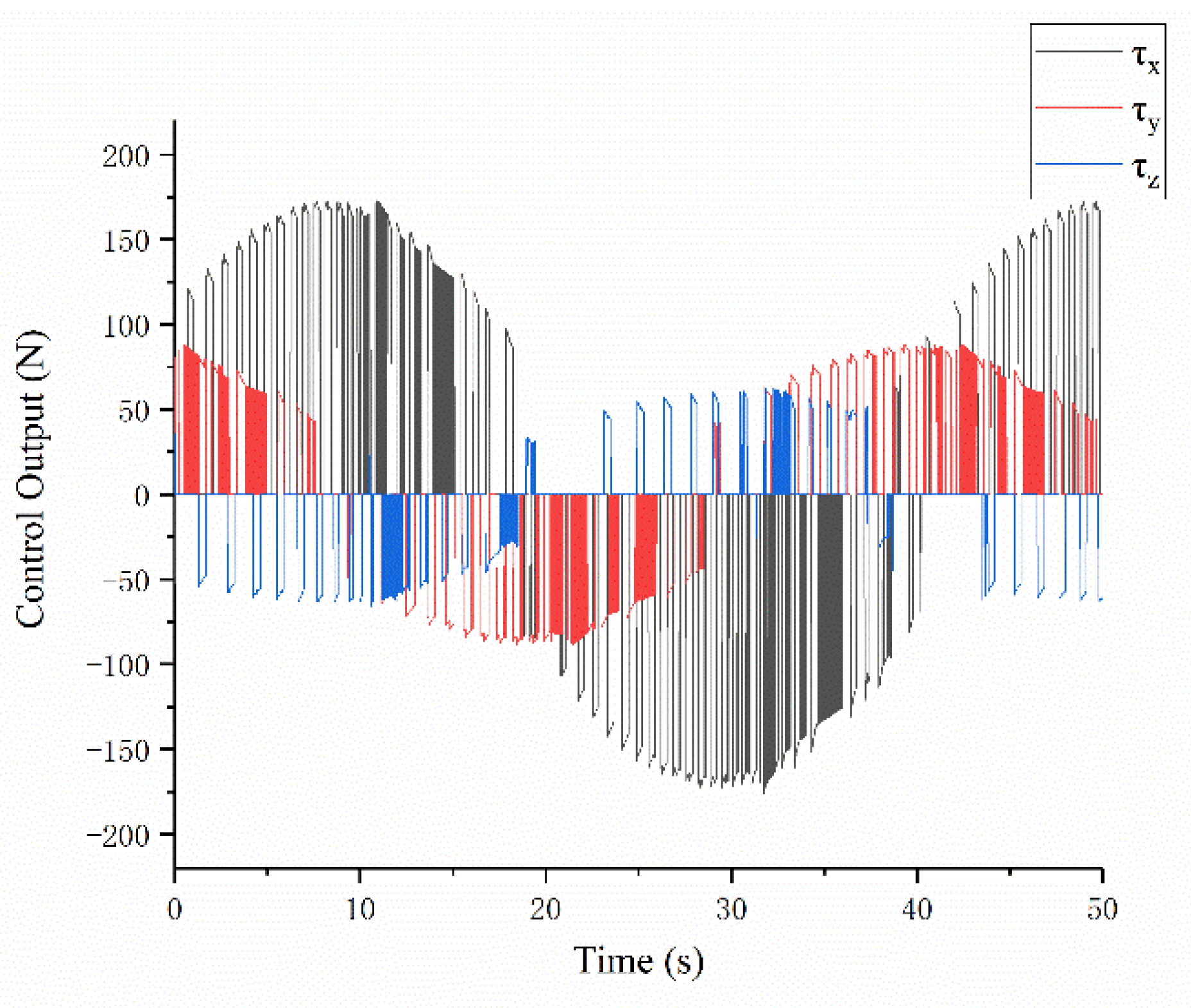
To calculate the energy consumption, the control output obtained is given first. Based on the above simulation process, the control outputs of two schemes are shown in Figure 7 and Figure 8.

In Figure 7 and Figure 8, the black, red, and blue lines represent the control output in the surge, sway, and heave directions, respectively.

To quantitatively analyze the effect of the schemes, the data in Figure 7 and Figure 8 are extracted. Then, the energy consumption is calculated by Equation (25). The specific data are presented in

Table 2. Performance of the PRTC scheme and traditional scheme in terms of energy consumption.

	Energy Consumption (105)
	Surge	Sway	Heave	Total
Traditional scheme	12.27	4.35	1.32	17.94
PRTC scheme	7.12	3.72	1.28	12.15

.

According to Table 2, compared with the traditional scheme, the energy consumption of the PRTC scheme in the three directions is reduced by 42.0%, 14.5%, and 3.0%, respectively, and the total energy consumption is reduced by 32.3%. Combined with Table 1, it can be seen that compared with the traditional scheme, the total energy consumption of this scheme is reduced by 32.3% without overshoot. It reflects the feasibility of the PRTC scheme in improving tracking accuracy and reducing energy consumption.

It can be seen from Figure 8 that the PRTC has the phenomenon of sudden change of control input signal on and off. Since the PRTC scheme considers the inertia of AUV for predictive control, it can be seen from Table 2 that the energy consumption of the PRTC scheme is better than that of the traditional scheme.

4.2.3. The Effect of Choices in Controller Parameters $k_1$ and $k_2$ on Energy Consumption

It can be seen from the control law (Equation (17)) that the selection of controller parameters $k_1$ and $k_2$ directly affects the control output. Since the energy consumption index is obtained by accumulating the control output (Equation (15)), it is necessary to analyze the effect of the controller parameters $k_1$ and $k_2$ on the energy consumption.

This section selects 4 sets of controller parameters: $k_1=0.6$,$k_2=0.2$;$k_1=0.8$,$k_2=0.3$; $k_1=1$, $k_2=0.4$; $k_1=1.2$, $k_2=0.5$, where $k_1\in R^{6\times 1},k_2\in R^{6\times 1}$. Calculate the corresponding energy consumption, the mean and mean square deviation of the tracking error, and the percentage of energy consumption reduction compared with the traditional methods. The mean and mean square deviation of the tracking error are calculated to reflect the dispersion degree of the real trajectory in the desired region, which is shown in

Table 3. Energy consumption, mean value of tracking error, mean square deviation of tracking error, and percentage reduction of energy consumption compared with the traditional scheme under different controller parameter selection.

	Different Controller Parameter Selection
	${\mathit{k}}_1=0.6$$, {\mathit{k}}_2=0.2$	${\mathit{k}}_1=0.8$$, {\mathit{k}}_2=0.3$	${\mathit{k}}_1=1$$, {\mathit{k}}_2=0.4$	${\mathit{k}}_1=1.2$$, {\mathit{k}}_2=0.5$
Energy Consumption (×105)	10.56	11.14	12.07	12.81
Mean value of tracking error (mm)	−0.0029	−0.0007	−0.0027	−0.0019
Mean square deviation of tracking error (mm)	0.0296	0.0238	0.0215	0.0198
Percentage reduction in energy consumption (%)	41.14	37.90	32.72	28.60

.

It can be seen from Table 3 that the selection of controller parameters will affect the energy consumption of tracking control to a certain extent. There is a law that the smaller the controller parameter selection, the lower the energy consumption. Compared with the traditional method, this method can significantly reduce the energy consumption under different controller parameters. By comprehensively analyzing the indicators in Table 3, it can be concluded that selecting a smaller control parameter can better reduce energy consumption, but the dispersion of its real trajectory in the expected area will increase. On the contrary, selecting a larger control parameter will increase the energy consumption, but it can better constrain the AUV near the centerline of the desired area.

4.3. Digital Simulation Verification of Control Law Optimization Scheme Considering Desired Region Range

This section compares the PRTC scheme with the control law optimization scheme considering the expected region. To demonstrate that the control law optimization scheme can effectively avoid the influence of the desired region on the control output compared with the PRTC scheme, this section uses different desired region ranges to analyze the performance of the two schemes on the control output. Then, the performance of the two schemes in energy consumption is further analyzed.

4.3.1. Compare the Performance of the Two Schemes in Control Output

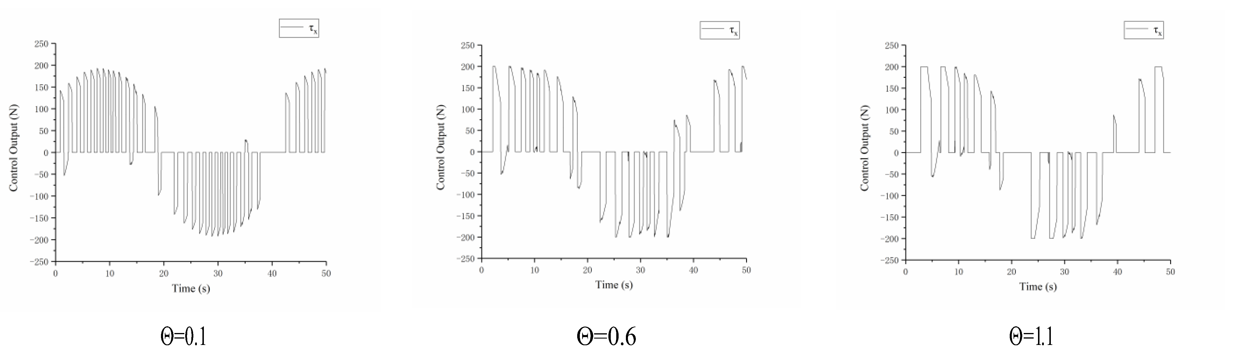
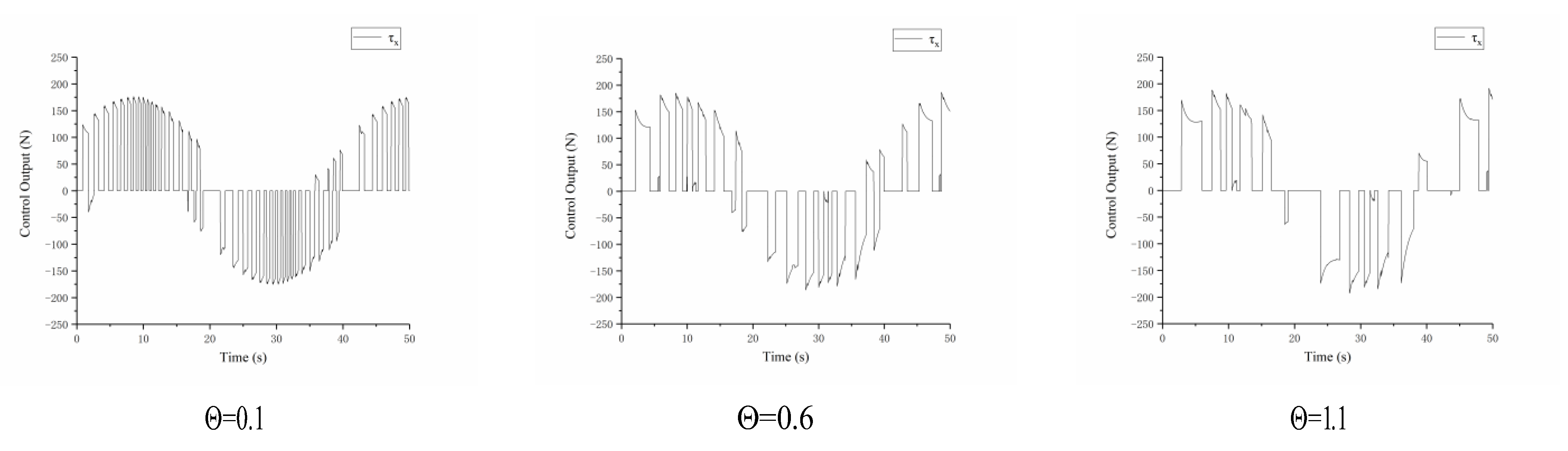
Based on different desired region ranges $\mathrm{\Theta }=[0.1,0.1,0.1,0,0,0{]}^T$, $\mathrm{\Theta }=[0.6,0.6,0.6,0,0,0{]}^T$, $\mathrm{\Theta }=[1.1,1.1,1.1,0,0,0{]}^T$(simply expressed as $\mathrm{\Theta }=0.1$, $\mathrm{\Theta }=0.6$, $\mathrm{\Theta }=1.1$), the control outputs of the two schemes are shown in Figure 9 and Figure 10.

In Figure 9 and Figure 10, the black line represents the control output in the surge direction.

As can be seen from Figure 9, as the desired region range expands, the control output also increases, and the time for the control output to reach saturation (${\tau }_{\max }=200$) is also longer. However, there is no significant change in the control output in Figure 10.

To quantitatively analyze the effect of the schemes, the number of steps that control output to reach saturation and the ratio of saturated steps to total control steps in Figure 9 and Figure 10 are extracted. The specific data are presented in

Table 4. Performance of PRTC scheme and control law optimization scheme in control output.

	Number of Steps That Control Output to Reach Saturation			Ratio of Saturated Steps to Total Steps (%)
	$\mathrm{\Theta }=0.1$	$\mathrm{\Theta }=0.6$	$\mathrm{\Theta }=1.1$	$\mathrm{\Theta }=0.1$	$\mathrm{\Theta }=0.6$	$\mathrm{\Theta }=1.1$
PRTC scheme	0	262	1064	0	2.6	10.64
Control law optimization scheme	0	0	0	0	0	0

.

According to Table 4, when the desired region ranges are $\mathrm{\Theta }=0.1$, $\mathrm{\Theta }=0.6$, and $\mathrm{\Theta }=1.1$, the number of steps that control output reach saturation are 0, 262, and 1064, respectively, accounting for 0, 2.6, and 10.64 of total control steps, respectively. It can be seen that with the expansion of the desired region, more control steps of the PRTC scheme are saturated. The control law optimization scheme considering the desired region range has no saturation in the desired region ranges, which are $\mathrm{\Theta }=0.1$, $\mathrm{\Theta }=0.6$, and $\mathrm{\Theta }=1.1$.

4.3.2. Compare the Performance of the Two Schemes in Terms of Energy Consumption

Extract the data in Figure 9 and Figure 10, and calculate the total energy consumption in the surge, sway, and heave directions through Equation (25). The specific data are presented in

Table 5. Performance of the two schemes in terms of energy consumption.

	Total Energy Consumption (105)
	$\mathsf{\Theta }=0.1$	$\mathsf{\Theta }=0.6$	$\mathsf{\Theta }=1.1$
PRTC scheme	12.15	12.85	12.08
Control law optimization scheme	11.70	11.83	11.12

.

Table 5 shows that compared with the PRTC scheme, the total energy consumption of the control law optimization scheme is reduced by 3.7%, 7.9%, and 7.9%. Combined with Table 2, it can be seen that compared with the PRTC scheme, the control law optimization scheme considering the desired region range can further reduce the total energy consumption without control output saturation. It reflects the feasibility of the control law optimization scheme in controlling output anti-saturation and reducing energy consumption.

4.4. Simulation Verification Considering the Uncertain Interference and Rapid Flow Perturbations

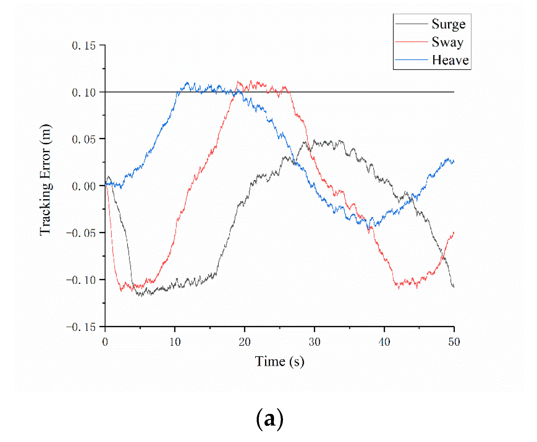
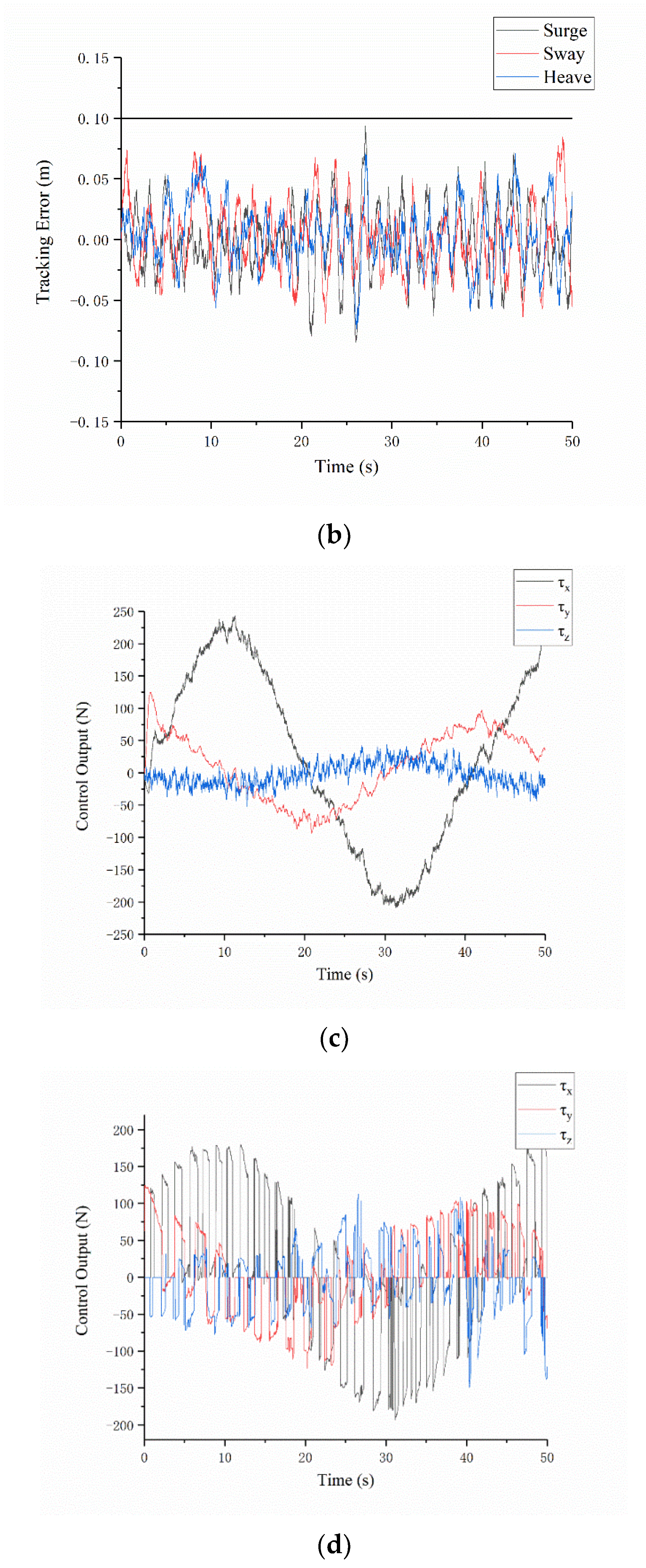
Considering that AUV will be affected by uncertainty, including sensor noise and flow perturbations under real conditions, the author adopts the method of filtering random numbers based on Gaussian distribution through first-order Butterworth filter and then superimposing them on controller input to sensor noise [19]. The first-order Gauss-Markov process is used to simulate flow perturbations [19]. The simulation results are shown in Figure 11.

As shown in Figure 11, in the case of uncertainty, the traditional scheme has overshoot, but the PRTC scheme has no overshoot. The control output of the traditional scheme fluctuates greatly, while the control output of the PRTC scheme fluctuates little.

In order to analyze the performance of disturbance on energy consumption, the data in Figure 11c, d are extracted to form

Table 6. Performance of the traditional scheme and the PRTC scheme in energy consumption under uncertainty.

	Energy Consumption (105)
	No Uncertainty	Without Uncertainty
Traditional scheme	17.94	18.26
PRTC scheme	10.66	13.40

.

According to Table 6, the energy consumption of the PRTC scheme is 59.42% of that of the traditional scheme without uncertainty, and 73.38% of that of the traditional method with uncertainty. This shows that the PRTC scheme can also reduce energy consumption in the case of uncertainty.

4.5. Results Discussion

To more clearly compare the qualitative and quantitative features of the proposed scheme and the traditional scheme, this section compresses all the results obtained to form

Table 7. Compare the qualitative and quantitative features of the proposed scheme and the traditional scheme.

	Qualitative Features		Quantitative Features
	Overshoot Judgement	Energy Consumption	Overshoot Time Accounts for the Total (%)			Maximum Overshoot (mm)			Total Energy Consumption (105)
			Surge	Sway	Heave	Surge	Sway	Heave
Traditional scheme	Yes	High	29.27	24.82	7.70	+13.16	+8.25	+5.35	17.94
Proposed scheme	No	Low	0	0	0	−14.20	−29.65	−19.75	11.70

.

Summary based on Table 7. In terms of qualitative features: the traditional scheme will lead to overshoot and high energy consumption when tracking the desired region, while the PRTC scheme will not produce overshoot and the energy consumption is lower than the traditional scheme; in terms of quantitative features: traditional scheme: the ratio of overshoot time to total simulation time in the three directions of sway, surge, and heave is 29.27%, 24.82%, and 7.70%, respectively. The maximum distance by which the actual trajectory exceeds the desired region in three directions is 13.16 mm, 8.25 mm, and 5.35 mm, respectively. The total energy consumption is 17.94 × 10⁵. The PRTC scheme: the overshoot time in all three directions is 0, the actual trajectory is 14.20 mm, 29.65 mm, and 19.75 mm closest to the outer boundary of the desired region. The total energy consumption is 11.70 × 10⁵, which is 34.78% lower than the traditional scheme.

5. Conclusions

In this paper, the problem of AUV region tracking is studied. Aiming at the problem of overshoot in traditional region tracking schemes, a prediction-based AUV region tracking (PRTC) scheme is proposed. The PRTC scheme realizes prediction control based on the relative motion relationship between AUV and the outer boundary of the desired region. The digital simulation results show that the PRTC scheme can realize the region tracking without overshoot. The digital simulation results show that compared with the traditional scheme, the energy consumption of the PRTC scheme in the three directions of sway, surge, and heave is reduced by 42.0%, 14.5%, and 3.0%, respectively, and the total energy consumption is reduced by 32.3%. In addition, because the PRTC scheme is different from the traditional scheme, it adds the control process to make the AUV return to the center of the desired region, resulting in the control output of the PRTC scheme being affected by the range of the desired region. As the range of the desired region increases, the control output saturation becomes more serious. To solve this problem, this paper proposes a control law optimization scheme considering the desired region. By transforming the error variables in the original scheme, the influence of the desired region on the control output of PRTC is eliminated. Theoretical analysis and simulation results show that the control output of the optimized control law is not affected by the desired region, and the energy consumption is reduced by 3.7% compared with that before control law optimization.

Deficiency of proposed method and further work plan: (1) the supplementary simulation in this paper shows that, in the presence of uncertainty, although the performance of the proposed scheme in the paper in terms of energy consumption is still better than that of the traditional scheme, the reduction of energy consumption is less than that without uncertainty. Therefore, in the next step, the authors will study how to achieve the goal of keeping low energy consumption while tracking the desired region in the presence of uncertainty. (2) In addition, the performance of the proposed scheme in flow perturbations and rapid changes of the medium, say pycnocline, also needs to be further studied.

References

- Guerrero, J.; Torres, J.; Creuze, V.; Chemori, A. Trajectory Tracking for Autonomous Underwater Vehicle: An Adaptive Approach. Ocean Eng. 2019, 172, 511–522. [Google Scholar] [CrossRef] [Green Version]
- Zereik, E.; Bibuli, M.; Mišković, N.; Ridao, P.; Pascoal, A. Challenges and Future Trends in Marine Robotics. Annu. Rev. Control 2018, 46, 350–368. [Google Scholar] [CrossRef]
- Tabataba’i-Nasab, F.S.; Keymasi Khalaji, A.; Moosavian, S.A.A. Adaptive Nonlinear Control of an Autonomous Underwater Vehicle. Trans. Inst. Meas. Control 2019, 41, 3121–3131. [Google Scholar] [CrossRef]
- Dai, Y.; Yu, S.; Yan, Y.; Yu, X. An EKF-Based Fast Tube MPC Scheme for Moving Target Tracking of a Redundant Underwater Vehicle-Manipulator System. IEEE/ASME Trans. Mechatronics 2019, 24, 2803–2814. [Google Scholar] [CrossRef]
- Xiao, B.; Yang, X.; Karimi, H.R.; Qiu, J. Asymptotic Tracking Control for a More Representative Class of Uncertain Nonlinear Systems with Mismatched Uncertainties. IEEE Trans. Ind. Electron. 2019, 66, 9417–9427. [Google Scholar] [CrossRef]
- Sun, W.; Su, S.F.; Wu, Y.; Xia, J.; Nguyen, V.T. Adaptive Fuzzy Control with High-Order Barrier Lyapunov Functions for High-Order Uncertain Nonlinear Systems with Full-State Constraints. IEEE Trans. Cybern. 2020, 50, 3424–3432. [Google Scholar] [CrossRef] [PubMed]
- Cheah, C.C.; Sun, Y.C. Adaptive Region Control for Autonomous Underwater Vehicles. In Proceedings of the Oceans ′04 MTS/IEEE Techno-Ocean ′04 Conference, Kobe, Japan, 9–12 November 2004; IEEE: New York, NY, USA. [Google Scholar]
- Cheah, C.C.; Sun, Y.C. Region Reaching Control for Robots with Uncertain Kinematics and Dynamics. Proc. - IEEE Int. Conf. Robot. Autom. 2006, 2006, 2577–2582. [Google Scholar] [CrossRef]
- Chu, Z.; Zhu, D. Fault-Tolerant Control of Autonomous Underwater Vehicle Based on Adaptive Region Tracking. J. Shandong Univ. Eng. Sci. 2017, 47, 57–63. [Google Scholar]
- Ismail, Z.H.; Faudzi, A.A.; Dunnigan, M.W. Fault-Tolerant Region-Based Control of an Underwater Vehicle with Kinematically Redundant Thrusters. Math. Probl. Eng. 2014, 2014, 527315. [Google Scholar] [CrossRef]
- Liu, X.; Zhang, M. Region Tracking Control for Autonomous Underwater Vehicle with Control Input Saturation. In Proceedings of the 39th Chinese Control Conference (CCC), Shenyang, China, 27–29 July 2020; IEEE: New York, NY, USA. [Google Scholar]
- Sun, X.; Ge, S.S. A DSC Approach to Adaptive Dynamic Region-Based Tracking Control for Strict-Feedback Non-Linear Systems. IET Control Theory Appl. 2022, 16, 94–111. [Google Scholar] [CrossRef]
- Liu, X.; Zhang, M.; Wang, S. Adaptive Region Tracking Control with Prescribed Transient Performance for Autonomous Underwater Vehicle with Thruster Fault. Ocean Eng. 2020, 196, 106804. [Google Scholar] [CrossRef]
- Ismail, Z.H.; Dunnigan, M.W. Tracking Control Scheme for an Underwater Vehicle-Manipulator System with Single and Multiple Sub-Regions and Sub-Task Objectives. IET Control Theory Appl. 2011, 5, 721–735. [Google Scholar] [CrossRef] [Green Version]
- Zhang, M.; Liu, X.; Wang, F. Backstepping Based Adaptive Region Tracking Fault Tolerant Control for Autonomous Underwater Vehicles. J. Navig. 2017, 70, 184–204. [Google Scholar] [CrossRef]
- Qiao, L.; Zhang, W. Adaptive Second-Order Fast Nonsingular Terminal Sliding Mode Tracking Control for Fully Actuated Autonomous Underwater Vehicles. IEEE J. Ocean. Eng. 2019, 44, 363–385. [Google Scholar] [CrossRef]
- Wang, M.; Wang, Z.; Chen, Y.; Sheng, W. Adaptive Neural Event-Triggered Control for Discrete-Time Strict-Feedback Nonlinear Systems. IEEE Trans. Cybern. 2020, 50, 2946–2958. [Google Scholar] [CrossRef] [PubMed]
- Mukherjee, K.; Kar, I.N.; Bhatt, R.K.P. Region Tracking Based Control of an Autonomous Underwater Vehicle with Input Delay. Ocean Eng. 2015, 99, 107–114. [Google Scholar] [CrossRef]
- Fossen, T.I. Handbook of Marine Craft Hydrodynamics and Motion Control; John Wiley & Sons Ltd: Noida, India, 2011; pp. 200–224. [Google Scholar]
Figure 1.
Schematic diagram of the PRTC scheme.
Figure 2.
Flow chart of the PRTC scheme.
Figure 3.
The relationship of parameters in the PRTC scheme.
Figure 4.
Schematic diagram of control law optimization scheme.
Figure 5.
Tracking error of traditional scheme.
Figure 6.
Tracking error of PRTC scheme.
Figure 7.
Control output of traditional scheme.
Figure 8.
Control output of PRTC scheme.
Figure 9.
Figure 10.
Control output of control law optimization scheme.
Figure 11.
Performance of PRTC scheme and traditional scheme considering uncertain interference and rapid flow perturbations. (a) Tracking error of traditional scheme; (b) tracking error of PRTC scheme; (c) control output of traditional scheme; (d) control output of PRTC scheme.