CFD Simulations of the Effect of Equalizing Duct Configurations on Cavitating Flow around a Propeller

Abstract

This study presented the results of a computational study of cavitating flows of a marine propeller with energy saving equalizing ducts. The main purpose of the study was to estimate the cavitating flows around a propeller with a duct, and to investigate the interaction between a duct and a propeller in cavitating flows. The INSEAN E779A propeller was used as a baseline model. Validation studies were conducted for non-cavitating and cavitating flows around a hydrofoil and a propeller. A comparison with the experimental data showed good agreement in terms of sheet cavity patterns and propulsion performances of the propeller. Various duct configurations have been presented, and it was found that a duct in front of the propeller had effects on the propeller’s cavitation and propulsion performance. Higher angles of attack of the duct showed a significant effect on the propeller’s cavitation behavior, especially with a small duct. The small duct lowered the cavitation inception radius with increase in angle of attack of the duct, while the large duct had more effect on the tip cavitation. The propeller with large duct gave higher thrust, however, the higher torque loading affected the propeller efficiency. Overall, it was found that the propeller with small duct provided a higher propeller efficiency

1. Introduction

The need to reduce carbon emissions through the enforcement of the energy efficiency design index (EEDI) by the International Maritime Organization (IMO) has led to a focus on further improvements of the hydrodynamic performance of ship propulsion systems. Consequently, this has resulted in the growth of research and development of energy saving devices (ESD) as an effective method to improve the overall propulsive performance of the ship.

ESDs are classified based on their operation principles and on how they modify flow around the propeller. To enhance propeller efficiency, duct type ESDs, pre-swirl fins devices, and post swirl fins have been developed, among others. Celik [1] studied the effectiveness of a wake equalizing duct (WED). Sakamoto et al. [2] investigated the working of a stern duct in model and full scale using CFD with overset grid arrangement. Pre-swirl Stator devices are mounted upstream of the propeller and modify the flow to the propeller. Park et al. [3] studied model and full-scale prediction of pre-swirl stator (PSS) using CFD simulation. Koushan et al. [4] developed a PSS through model tests with power saving from the device. Post-swirl devices are installed behind the propeller and are designed to cancel the rotational flow in the slipstream of the propeller. Studies on flows around a propeller boss cap fin (PBCF) were carried out [5,6]. In other instances, duct and pre-swirl stators have been combined to enable improved performance. Mewis [7] developed the WED combined with pre-swirl fins.

Ducts are installed on the upstream of a ship’s propeller to increase the flow to a propeller during operation at sea. Terwisga [8] argued that the reason to install a duct around a propeller is because it contributes to the overall efficiency by acceleration of flow through the propeller plane, thereby increasing the mass flux through the propeller which gives rise to the ideal efficiency. These effects of a duct on propeller performance in non-cavitating flows have been investigated [9,10]). Go et al. [9] numerically investigated the effects of a duct on propeller performance considering a wide range of diameters and angles of attack of the duct. Lungu A. [10] used ISIS-CFD unsteady viscous solver to conduct simulations on the effects of nozzles placed in front of propellers.

Cavitation simulations of marine propellers using numerical methods have become more reliable due to the development of computer power and respective numerical methods for computations. Park et al. [11] captured low pressure and phase changes based on the Reynolds-averaged Navier–Stokes (RANS) equations, and Bensow [12] described dynamic cavitation behavior based on large eddy simulations (LES). Based on the literature provided, there has been limited research on cavitation of marine propeller with a duct placed upstream. However, the study of cavitation on this setup will enable a better understanding of the change in cavitation behavior of the propeller under uniform flow conditions when the duct was placed on the upstream of the propeller in the open water test setup.

INSEAN E779A, a marine propeller, has been investigated numerically when an energy saving duct was installed upstream of the propeller. Uniform flow under both non-cavitating and cavitating conditions have been studied. The cavitation characteristics and performances of the propeller with a duct have been compared to those of the case without a duct. To simulate non-cavitating and cavitating flows, an open source CFD library, called OpenFOAM, was selected. The cavitating flow solver using the OpenFOAM platform has been applied to many cavitating flows [13,14,15,16,17,18,19].

2. Computational Methods

2.1. Governing Equations

The governing equations used for the simulations of the non-cavitating and cavitating flows around a propeller were the continuity and Navier–Stokes equations. These equations are expressed as follows:

$$\nabla ·U=\dot{m}\left(\frac{1}{{\rho }_v}-\frac{1}{{\rho }_l}\right)$$

(1)

$$\frac{\partial \left(\rho U\right)}{\partial t}+\nabla ·\left(\rho UU\right)=-\nabla p+\nabla ·\tau +S$$

(2)

where, $\rho$ is the fluid density, $p$ is the pressure, $\dot{m}$ is the interphase mass transfer, ${\rho }_v$ is the vapor density, and ${\rho }_l$ is the liquid density.

The cavitation model proposed by Schnerr and Sauer [20] was employed in this simulation due to its stability. The model was based on the Rayleigh–Plesset equation for the bubble dynamics.

$$\frac{\partial \alpha }{\partial t}+\nabla ·\left(\alpha U\right)=\frac{\dot{m}}{{\rho }_v}$$

(3)

Here, $\alpha$ is the volume fraction and $\dot{m }$ is the interphase mass transfer. The mass transfer equation between the phases was a function of the saturation pressure (${\rho }_{sat}$). The interphase mass transfer is decomposed based on liquid mass growth due to vapor condensation and liquid evaporation.

$$\dot{m}=\{\begin{array}{c}{C}_C\frac{{\rho }_v{\rho }_l}{\rho }\alpha \left(1-\alpha \right)\frac{3}{R_B}\sqrt{\frac{2}{3}\frac{p-p_{sat}}{{\rho }_l}} , p>p_{sat}\\ -C_V\frac{{\rho }_v{\rho }_l}{\rho }\alpha \left(1-\alpha \right)\frac{3}{R_B}\sqrt{\frac{2}{3}\frac{p-p_{sat}}{{\rho }_l}}, p<p_{sat}\end{array}$$

(4)

Here, $C_C$ and $C_V$ are the condensation and evaporation coefficients. The value used for $C_v$ and $C_c$ was 1. The model’s bubble radius is

$$R_B=\sqrt[3]{\frac{3\left(1+{\alpha }_{Nuc}-\alpha \right)}{4\pi n_0\alpha }}$$

(5)

Nucleation fraction (${\alpha }_{Nuc}$) is obtained from ${\alpha }_{Nuc}=\frac{V_{Nuc}}{1+V_{Nuc}}$. Here, the nucleation volume, $V_{Nuc}=\frac{\pi n_0{d}_{Nuc}^3}{6}$. The input parameters for the model are the nucleus density $n_0=1.6\times {10}^9$ and the initial nucleus diameter $d_{Nuc}=2.0\times {10}^{-8}$.

2.2. Numerical Methods

Spatial derivatives used second order accurate schemes as well as the time evolution. The analyses were done using segregated solver, with PIMPLE algorithms (Lee and Park, [21]) applied for coupling of pressure and velocity fields that allows stable transient simulations. To close the RANS equation, k-w SST turbulence model was used. The discretized equations were solved using a pointwise Gauss–Seidel iterative method, while a geometric agglomerated algebraic multi-grid algorithm was selected to accelerate solution convergence.

3. Problem Description

INSEAN E779A is a four bladed fixed pitch propeller [22]. Key specifications of the propeller are shown in

Table 1. INSEAN E779A principal particulars.

No. of Blades	4
Diameter (m)	0.227227
Pitch ratio (P/D) at r/R = 0.7	1.1
Pitch (P) (m)	0.15225
$\mathrm{Expanded}\mathrm{area}\mathrm{ratio}(A_E/A_0$)	0.69

.

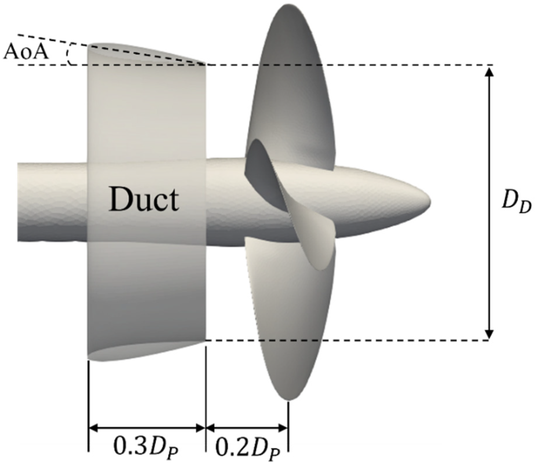
Figure 1 shows the propeller and duct configuration. The duct was made of a NACA0015 hydrofoil section. The chord length of the duct was 0.3$D_P$ and it was placed at a distance 0.2$D_P$ from the propeller plane. Here, $D_P$ is the propeller diameter. The duct outlet diameter ($D_D$) was used for adjusting the size of the duct where $0.7D_P\le D_D\le 1.0D_P$. The duct had a set of five angles of attack (AoA) ranging from 0° to 20° which were increased in increments of 5°. The computational domain had a cylindrical shape, and the flow’s directional length was 2.5$D_P$ upstream and 3$D_P$ downstream.

At the inlet boundary, Dirichlet condition was imposed for the incoming velocity, whereas at the outlet boundary, Neumann condition for pressure was imposed. The value of velocity at the inlet was equivalent to the freestream velocity ($U_{\infty })$. On the duct’s surface, the no-slip condition was imposed. The propeller and shaft hub were imposed with moving wall boundary conditions.

Computational meshes are key for reliable predictions, especially in investigation of cavitation. Therefore, an accurate discretization near the walls was done with fine mesh around the propeller blades and hub of the propeller [23]. Areas around the tip of the propeller was refined to accurately capture the tip vortices. Mesh layers were added to the propeller blade. SnappyHexMesh, a meshing tool built into OpenFOAM, was used for meshing as shown in Figure 2. To rotate the propeller, the arbitrary mesh interface (AMI) technique was used. The simulation used a mesh count of 2,669,759 cells.

4. Results and Discussion

4.1. Propeller Open Water Test in Non-Cavitating Flow

Prior to beginning cavitation simulations, the CFD results were validated against the experimental open water test results [22].

Table 2. Open water test results.

	${\mathit{K}}_{\mathit{T}}$			$10{\mathit{K}}_{\mathit{Q}}$			${\eta }_0$
$\mathit{J}$	Experiment (Salvatore et al. [22])	Present	Difference (%)	Experiment (Salvatore et al. [22])	Present	Difference (%)	Experiment (Salvatore et al. [22])	Present	Difference (%)
0.099	0.508	0.492	3.150	0.829	0.802	3.257	0.097	0.097	0.111
0.298	0.430	0.428	0.465	0.707	0.709	0.283	0.288	0.286	0.746
0.498	0.340	0.339	0.294	0.574	0.577	−0.523	0.469	0.466	0.813
0.695	0.245	0.239	2.449	0.438	0.461	−5.251	0.619	0.573	7.316
0.895	0.150	0.147	2.000	0.294	0.302	−2.721	0.727	0.693	4.596
0.970	0.111	0.105	5.450	0.234	0.221	5.556	0.732	0.733	−0.159
1.094	0.044	0.042	5.000	0.135	0.238	5.926	0.567	0.573	−0.984

shows the open water test results without a duct. Deviation from the experimental results for the thrust coefficient $\left(K_T\right)$ ranged from 0.294% to 5.45%, while for the torque coefficient $\left(K_Q\right)$ it ranged from 0.283% to 5.926%; therefore, the deviations had an overall underestimation.

4.2. Hydrofoil in Two-Dimensional (2D) Cavitating Flow

To validate a 2D cavitating flow, a cavitating flow around the 2D modified NACA66 hydrofoil with an angle of attack (AoA) of four degrees was considered [14]. The hydrofoil was considered for leading edge cavitation, which is normally synonymous with propeller cavitation. It was observed that the cavitation inception could be predicted based on pressure distribution, since cavitation occurred at the minimum pressure coefficient ($C_P=\frac{p-p_{ref}}{0.5\rho U_{\infty }^2}$), where the cavitation number ($\sigma$) is expressed as

$$\sigma =\frac{p-p_{sat}}{0.5\rho U_{\infty }^2}$$

(6)

The cavitation characteristics for the hydrofoil section were described by the minimum pressure envelope as a function of the cavitation number. Figure 3 shows the pressure coefficient distribution on the modified NACA66 hydrofoil section’s surface when the cavitation number is 0.84. Compared with the experimental data [24], the present result captured the cavity close and pressure distribution well.

4.3. Propeller in Three-Dimensional (3D) Cavitating Flow

To simulate a 3D cavitating flow, the experiment data for the INSEAN E779A propeller at $J=0.71$ and ${\sigma }_n=1.763$ [22] was selected. The propeller cavitation number based on the rotation speed is obtained as follows

$${\sigma }_n=\frac{p-p_{sat}}{0.5\rho {\left(n{D}_P\right)}^2}$$

(7)

where, $n$ is the number of revolutions per second. The predicted cavitations on the propeller blade for various nucleus densities are shown in Figure 4. The sheet cavitation is the pronounced type of cavitation. The experimental blade cavitation shows little difference from the simulation cases without a duct since selected numerical methods have difficulty in showing the bubble cavitation observed on the experiments. The inception of both simulation and experiment occurred on the leading edge of the propeller blade, therefore showing some similarity. In the cavitation model, the nucleation density was critical in determination of the cavitation behavior. Various nucleus densities were used. For a higher density, sheet cavitation was overestimated. The cavity extent over the trailing edge was increased for the higher nucleation density [25]). For simulations of all other cases, the nucleus density of $1.6\times {10}^9$ was used.

In

Table 3. Propeller propulsion coefficients for the case without duct and cavitation condition.

	${\mathit{K}}_{\mathit{T}}$			$10{\mathit{K}}_{\mathit{Q}}$
	Experiment (Salvatore et al. [22])	Present	Difference (%)	Experiment (Salvatore et al. [22])	Present	Difference (%)
Cavitation Test	0.255	0.240	5.882%	0.460	0.423	8.043%

, for the cavitation case at $J=0.71$ and ${\sigma }_n=1.763$, the thrust and torque coefficients were 5.882% and 8.043%, respectively, less than the experiment. This could be attributed to cavitation blockage effects not being included in the CFD [25].

4.4. Propeller with Duct in Cavitating Flow

Figure 5 and Figure 6 show instantaneous non-dimensional axial velocity contours on the y=0 plane when the blade indicates 0 degrees. The flow was accelerated through the duct. The propeller’s incoming flow speed increased near the propeller and a low-speed region was formed at the wake of the duct. The low-speed region was more evident in ducts with a high angle of attack for both sizes of duct. The slipstream was axis-symmetrical about the axis of the propeller. The axial velocity was observed to be larger in the slipstream region and was relatively smaller near the blade tips and the axis of the propeller. In the outer region of the duct, the flow was under low speed while in the inner region of the duct the flow was under high speed. These two regions could be clearly distinguished, especially when varying from a small angle of attack to a large angle of attack. The duct with the highest angle of attack gave a strong wake that was increasing with the increase in the angle of attack of the duct, as shown in Figure 5e and Figure 6c,d. However, when flows had a higher angle of attack and ducts had large diameter ($D_D=D_P$), flow instabilities could be observed downstream in Figure 6c,d. This could be related to the strong wake that was formed on the tip of the propeller.

To study flow characteristics, three locations are selected as shown in Figure 7. The selected locations ($x/R$) were −0.5, 0 (propeller plane), and 1.5. Here, $R$ is the propeller radius.

Figure 8 and Figure 9 show instantaneous non-dimensional axial velocity contours on transverse plane for $D_D=0.7D_P$ and $D_D=D_P$, respectively. The accelerated flows were observed at $x/R=-0.5$. The velocity distribution generally tended to increase gradually along the radial direction from the center position to the extreme end of blade, which could be attributed by the rotary action of the propeller. At the propeller plane ($x/R$ = 0), the velocity gradient was clearly seen. Comparing the flow generated from the two sizes of the ducts, differences in the flow fields with respect to the angle of attack were observed mainly near the wakes of the ducts. There was a more evident and distinct tendency, as the angle of attack increased due to the change of the slipstream. The boundary between the slipstream and the freestream was smoother for the propeller without the duct compared to the case with the duct. This was because flow separation occurred near the trailing edge of the duct where the vortices generated from the duct strongly interacted with the blade tip vortices. The chaotic boundary of the slipstream could be clearly seen from the duct with $\mathrm{AoA}={20}^o$ in Figure 9d through plane ($x/R$ = 0). In the small duct ($D_D=0.7D_P$), the flow was separated at $r/R=0.7$, causing a different inflow to the propeller blade. The flow gradient at the propeller plane for the small duct was evident compared to the large duct ($D_D=D_P$). This flow gradient was more evident on the case with large AoA. The flow gradient was not dominant at the slipstream far from the propeller plane, as it diminished.

Figure 10 and Figure 11 show the pressure coefficient contours at y = 0 plane for the cases with $D_D=0.7D_P$ and $D_D=D_P$, respectively. The pressure coefficient showing a value of $C_P=-1.763$ represented regions with pressure lower than the saturation pressure. A distinct decrease in the pressure coefficient on the suction side of the propeller was caused by the suction effect of the propeller on the inbound flow resulting in pressure below the vapor pressure and therefore cavitation. The low-pressure area was where the lowest value of $C_p$ was equivalent to the cavitation number, and was dependent on the angle of attack. A higher pressure around the propeller tip on the pressure side increased with the increasing angle of attack of the duct, regardless of the size of the duct.

Figure 12 shows the cavitation shape for the propellers with $D_D=0.7D_P$. The vapor fraction of 0.5 was selected to visualize the cavity interface. Sheet cavitation was incepted at the leading edge and propagated to the downstream on the blade. The sheet cavitation was dominant on the suction side, with increased angles of attack. As the angle of attack increased, the cavitation inception radius decreased, indicating a large cavitation area. For $D_D=0.7D_P$, the inception points for AoA = 5° was observed to be approximately $r/R=0.75,$ while the inception point for AoA $=20°$ was approximately $r/R=0.65$. Figure 13 shows the cavitation shape for the propellers with $D_D=D_P$. A high angle of attack of the large duct increased cavitation around the tip region. The cavitation inception point moved up as compared to the propeller without the duct. The inception points of the case with $D_D=D_P$ and AoA = 5° was observed to be approximately $r/R=0.75,$ while for the case with $\mathrm{AoA}=20°$, the inception point was observed to be at approximately $r/R=0.8$.

Figure 14 represents the thrust and torque coefficients for different angles of attack. Regardless of the size of the duct, as angle of attack increased, there was an increase in both the coefficients of thrust and torque compared to the propeller without the duct. The large duct caused higher thrust and torque than the small duct in all angles of attack under the cavitating condition. The large cavitation area in the small duct reduced the thrust and torque compared to the large duct. The propeller equipped with ducts provided a higher thrust and torque compared to the propeller without a duct. Regardless of the size, all ducts showed increased thrust and torque with higher angles of attack. From the propeller efficiency in Figure 14c, for small angle of attack of both size of the ducts, there was negligible change in the propeller efficiency compared to the case without duct. As the angle of attack increased, the ducts show striking contrast in that the small duct increased the efficiency while the large duct decreased the efficiency. When the large duct had a higher angle of attack above 15°, there was a faster inflow into the propeller than in case with small duct and without duct. This simultaneously burdened the torque of the propeller resulting in the large duct having lower propeller efficiency.

5. Conclusions

This study numerically investigated the effect of ducts when placed upstream of a propeller. The INSEAN 779A propeller was selected in this study.

For the validation of cavitating flows, a cavitation model based on a homogeneous mixture model (Schnerr and Sauer, 2001) was selected. The cavitating flows around the 2D modified NACA66 hydrofoil and the 3D INSEAN 779A propeller were simulated and the pressure distribution, propulsion performances and cavitation shape were compared with experimental data.

The cavitation behavior of the marine propeller was seen to change when a duct was installed upstream. Different duct sizes and angles of attack were considered. For the cavitating flows with a higher angle of attack and duct with a large diameter ($D_D=D_P$), a strong unstable wake was seen downstream of the duct and interacted with the tip vortices of the propeller. In terms of the duct size ($D_D=0.7D_P$), the most dominant cavitation was sheet cavitation that extended to the back face of the propeller. The sheet cavitation area was observed to increase with increased angle of attack. In the propeller with the large duct, sheet cavitation was observed to lean toward the tip and leading edge with the increase in the angle of attack. For the propeller with the large duct, cavitation inception began around $r/R=0.75$ of the propeller as compared to the small duct whose inception radius extended up to $r/R=0.75$. As the angle of attack increased, cavitation was extended around the tip of the propeller. The cavitation inception radius was seen to depend on the size of the duct and angle of attack of the duct. A large duct had a bigger inception radius as compared to the small duct.

The large duct provided a higher thrust than the small duct however this was cancelled by the large torque loading experienced on the propeller. Consequently, the large duct experienced lower propeller efficiency compared to the propeller with small duct.

References

- Celik, F. A numerical study for effectiveness of a wake equalizing duct. Ocean Eng. 2007, 34, 2138–2145. [Google Scholar] [CrossRef]
- Sakamoto, N.; Kobayashi, H.; Ohashi, K.; Kawanami, Y.; Windén, B.; Kamiirisa, H. An overset RaNS prediction and validation of full-scale stern wake for 1,600TEU container ship and 63,000 DWT bulk carrier with an energy saving device. Appl. Ocean Res. 2020, 105, 102417. [Google Scholar] [CrossRef]
- Park, S.; Oh, G.; Rhee, S.H.; Koo, B.-Y.; Lee, H. Full Scale wake prediction of an energy saving device by using computational fluid dynamics. Ocean Eng. 2015, 101, 254–263. [Google Scholar] [CrossRef]
- Koushan, K.; Krasilnikov, V.; Nataletti, M.; Sileo, L.; Spence, S. Experimental and numerical study of pre-swirl stators PSS. J. Mar. Sci. Eng. 2020, 8, 47. [Google Scholar] [CrossRef] [Green Version]
- Kawamura, T.; Ouchi, K.; Nojiri, T. Model and full scale CFD analysis of propeller boss cap fins (PBCF). J. Mar. Sci. Technol. 2012, 17, 469–480. [Google Scholar] [CrossRef]
- Seo, J.; Lee, S.J.; Han, B.; Rhee, S.H. Influence of design parameter variations for propeller-boss-cap-fins on hub vortex reduction. J. Ship Res. 2016, 60, 203–218. [Google Scholar] [CrossRef]
- Mewis, F.; Guiard, T. Mewis duct–new developments, solutions and conclusions. In Proceedings of the 2nd International Symposium on Marine Propulsors, Hamburg, Germany, 15–17 June 2011. [Google Scholar]
- van Terwisga, T. On the working principles of Energy Saving Devices. In Proceedings of the Third International Symposium on Marine Propulsors, Tasmania, Australia, 5–8 May 2013. [Google Scholar]
- Go, J.; Yoon, H.; Jung, J. Effects of a duct before a propeller on propulsion performance. Ocean Eng. 2017, 136, 54–66. [Google Scholar] [CrossRef]
- Lungu, A. Energy-Saving Devices in Ship Propulsion: Effects of Nozzles Placed in Front of Propellers. J. Mar. Sci. Eng. 2021, 9, 125. [Google Scholar] [CrossRef]
- Park, S.; Heo, J.; Yu, B. Numerical study on the gap flow of a semi-spade rudder to reduce gap cavitation, J. Mar. Sci. Technol. 2010, 15, 78–86. [Google Scholar] [CrossRef]
- Bensow, R.E. Implicit LES predictions of the cavitating flow on a propeller. J. Fluids Eng. 2010, 132, 041302. [Google Scholar] [CrossRef]
- Park, S.; Rhee, S.H. Computational analysis of turbulent super-cavitating flow around a two-dimensional wedge-shaped cavitator geometry. Comput. Fluids 2012, 70, 73–85. [Google Scholar] [CrossRef]
- Park, S.; Rhee, S.H. Numerical analysis of the three-dimensional cloud cavitating flow around a twisted hydrofoil. Fluid Dyn. Res. 2013, 45, 015502. [Google Scholar] [CrossRef]
- Park, S.; Rhee, S.H. Comparative study of incompressible and isothermal compressible flow solvers for cavitating flow dynamics. J. Mech. Sci. Technol. 2015, 29, 3287–3296. [Google Scholar] [CrossRef]
- Gaggero, S.; Villa, D. Steady cavitating propeller performance by using OpenFOAM, StarCCM+ and a boundary element method. J. Eng. Marit. Environ. 2016, 231, 411–440. [Google Scholar] [CrossRef]
- Park, S.; Yeo, H.; Rhee, S.H. Isothermal compressible flow solver for prediction of cavitation erosion, Eng. Appl. Comput. Fluid Mech. 2019, 13, 683–697. [Google Scholar]
- Park, S.; Seok, W.C.; Park, S.T.; Rhee, S.H.; Choe, Y.; Kim, C.; Kim, J.H.; Ahn, B.K. Compressibility effects on cavity dynamics behind a two-dimensional wedge. J. Mar. Sci. Eng. 2020, 8, 39. [Google Scholar] [CrossRef] [Green Version]
- Lee, I.; Park, S.; Seok, W.; Rhee, S.H. A study on the cavitation model for the cavitating flow analysis around the marine propeller. Math. Probl. Eng. 2021, 2021, 2423784. [Google Scholar] [CrossRef]
- Schnerr, G.H.; Sauer, J. Physical and Numerical Modelling of Unsteady Cavitation Dynamics. In Proceedings of the 4th International Conference on Multiphase Flow, New Orleans, LA, USA, 27 May–1 June 2001. [Google Scholar]
- Lee, S.C.; Park, S. Platform Motions and Mooring System Coupled Solver for a Moored Floating Platform in a Wave. Processes 2021, 9, 1393. [Google Scholar] [CrossRef]
- Salvatore, F.; Pereira, F.; Felli, M.; Calcagni, D.; Di Felice, F. Description of the INSEAN E779A Propeller Experimental Dataset; Technical Report INSEAN 2006-085, Italian Ship Model Basin, Italy; Researchgate: Berlin, Germany, 2006. [Google Scholar]
- Ng’aru, J.M.; Park, S.; Hyun, B. Computational analysis of KCS model with an equalizing duct. J. Ocean Eng. Technol. 2021, 35, 247–256. [Google Scholar] [CrossRef]
- Shen, Y.; Dimotakis, P.E. The influence of surface cavitation on hydrodynamic forces. In Proceedings of the 22nd American Towing Tank Conference, St. John’s, NL, Canada, 8–11 August 1989. [Google Scholar]
- Shin, K.W.; Andersen, P. CFD Analysis of Ship Propeller Thrust Breakdown. In Proceedings of the 6th International Symposium on Marine Propulsors, Rome, Italy, 26–30 May 2019. [Google Scholar]
Figure 1.
Propeller and duct configuration.
Figure 2.
Typical mesh.
Figure 3.
Pressure coefficient distribution on 2D modified NACA66 hydrofoil surface at = 0.84.
Figure 4.
Cavitation on INSEAN E779A propeller blade for various nucleus densities (Salvatore et al., [22]).
Figure 5.
Instantaneous non-dimensional axial velocity contours on longitudinal plane for small duct ().
Figure 6.
Instantaneous non-dimensional axial velocity contours on longitudinal plane for large duct ().
Figure 7.
Flow measurement locations.
Figure 8.
Instantaneous non-dimensional axial velocity contours at = −0.5, 0, and 1.5 for (left: middle: ; right: ).
Figure 9.
Figure 10.
contours on longitudinal plane for cases with .
Figure 11.
Figure 12.
Cavitation of cases with .
Figure 13.
Figure 14.
Propeller performance coefficients.