Date-Driven Tracking Control via Fuzzy-State Observer for AUV under Uncertain Disturbance and Time-Delay

Abstract

This paper focuses on developing a data-driven trajectory tracking control approach for autonomous underwater vehicles (AUV) under uncertain external disturbance and time-delay. A novel model-free adaptive predictive control (MFAPC) approach based on a fuzzy state observer (FSO) was designed to achieve high precision. Concretely, the mathematical model of AUV motion was analyzed, and simplified via model decoupling, thus providing the model basis with an explicit physical explanation for the controller. Second, the MFAPC scheme for a multiple-inputs and multiple-outputs (MIMO) discrete time system was derived, that estimates system external disturbance. The controller can online estimate and predictive time-varying parameter pseudo-Jacobian matrix (PJM) to establish equivalent state space data-model for AUV motion system. Third, the Takagi–Sugeno (T–S) fuzzy model based state observer was designed to combine with the MFAPC scheme for the first time, which was used to online decline the state error generated by system uncertain time-delay. In addition, the stability of the proposed control scheme was analyzed. Finally, two trajectory tracking scenarios were designed to verify the effectiveness and robustness of the proposed FMFAPC scheme, and the simulations are implemented using the realistic parameters of T-SEA AUV.

1. Introduction

With the development of electronic hardware and the advancement of computer technology in recent decades, unmanned systems have played a significant role in numerous fields. Autonomous Underwater Vehicles (AUVs) are momentous types of unmanned marine crafts that are indispensable nowadays [1], including those that implement military reconnaissance, hydrological sampling, resource exploration, pipeline inspection, and fish aquaculture [2,3,4,5]. To ensure the advantages and performance of AUVs in the application field, high-accuracy trajectory tracking control is a crucial technique issue that needs to be solved [6].

Conventional-type AUVs are shaped like f a torpedo, are equipped with at least one paddle propeller or hydraulic propeller as a driver, and uses rudders and flanks to control their attitudes. Compared with other types of unmanned crafts, the operating environment of an AUV is complex and changeable, with random disturbances such as water currents and surges. These external disturbances will make the motion of AUV’s attitudes unstable and cause it to sideslip. To solve this issue, researchers apply adaptive control to estimate the motion deviations caused by external currents. In [7], a novel predictor-based line-of-sight (PLOS) guidance law was presented to rapidly identify and compensate for the sideslip angles of the vehicle. In [8], a terminal sliding mode control (SMD) approach was developed for AUVs, aiming to mitigate and solve unknown disturbances in the underwater environment. Gun et al. [9] proposed a back-stepping approach to handle the nonlinear dynamics of the vehicle, including sea currents and external disturbances.

Due to the unpredictable nature of the hydrological environment, it is difficult to build an accurate mathematical model or obtain precise model parameters for the AUV motion system [10,11], which is the basis for the control algorithm. In this case, the performance of the model-based control scheme was seriously degraded. Given this issue, a model-based control scheme with high accuracy and robustness is challenging. Yet, data-driven control approaches utilize online input-output (I/O) data to directly generate and self-adjust the controller, this control approach is also called as model-free control approach. Model-free adaptive control (MFAC) is a novel control approach that was developed based on the data-driven concept, and can handle the control issues caused by an inaccurate mathematical model or imprecise system parameters [12,13,14]. The MFAC scheme uses a dynamic linearization technique to build the equivalent data model rather than just using measurement I/O data to generate the controller. In this case, prior training is not required for the MFAC controller. From the application point of view, the MFAC is practical. Many researchers have worked in recent years to improve MFAC on a theoretical level and to apply it to unmanned systems. In [15], the MFAC scheme was combined with an adaptive factor to reduce system oscillation and overshoot for accomplishing unmanned surface vehicle heading control. Yue et al. [16] developed an improved MFAC via particle swarm optimization (PSO) algorithm for the unmanned ground vehicle to overcome the influence of time-delay and sudden wheelbase change. In [17], a novel improved MFAC scheme was proposed for spacecraft, aim at ensure controller parameters could adjust adaptively. An SMC scheme was combined with MFAC to strengthen the robustness of tracking performance. Meanwhile, the research on MFAC and its improved algorithm to practice on AUV is still rare, but on drawing previous research results, practicing MFAC on AUV is meaningful and appropriate.

With respect to the MFAC algorithm, it relies on a mathematical quantity, namely, the pseudo-Jacobian matrix (PJM), to describe the dynamic changes of multiple inputs and multiple outputs (MIMO) system, and builds the equivalent approximate data model. However, the complex MIMO system is likely to have parameters that jump or are subjected to external random disturbance, magnifying the model approximation error [18] between the data model and the actual system, which cannot be ignored.

Additionally, the time-delay phenomenon widely exists in practical operating systems. The controller cannot inhibit the disturbance timely when the system is subjected to a time-delay, the control system is prone to generating excessive overshoot and will undermine dynamic control performance. A nonlinear systems can be expressed by the Takagi-Sugeno (T-S) fuzzy modeling approach, and divide the system into numerous linear subsystems associated with fuzzy membership functions, which is aimed at simplifying the complex nonlinearity of the actual system [19,20,21]. In recent decades, the T-S fuzzy modeling technique has become a significant approach for processing nonlinear control issues and also an important means of handling system time-delay [22,23]. Many research results have demonstrated with the time-delay issue in nonlinear dynamic systems [24,25,26]. In [27], considering time-varying delay and input constraint, a novel control approach was proposed based on the T-S fuzzy model expressed system, and researchers performed simulation on a flexible-joint robot to verify its utility. The stabilization problem of flexible spacecraft was addressed based on saturated time-delay input via the T-S fuzzy model [28]. Zhong et al. [29] developed an effective approach to attenuate the impact of the unknown output-delay via the T-S fuzzy model -based augmented observer for the unmanned vehicle. Generally, the controller of a practical system is not only subjected by the unknown time-delay, but also affected by external disturbance. Thereby, considering both time-delay and external disturbance simultaneously is practical and generalized.

Inspired by previous research results, in this paper we study the trajectory tracking technique for AUVs. An improved control scheme based on model-free adaptive control was designed, aiming to handle the influence of external uncertain disturbances. Moreover, we designed a discrete T-S fuzzy model-based state observer to deal with the system’s uncertain time-delay. The main contributions of this study are summarized as follows:

• A novel tracking controller was proposed via improved model-free adaptive predictive control (MFAPC) for AUV horizontal sailing. The dynamic linearization method and predictive control concept were utilized to design an MFAPC controller. We utilized the dynamic linearization method and predictive control concept to design an MFAPC controller. Combining the MFAPC approach with the fuzzy state observer (FSO), we realized accurate tacking control under system time-delay and external disturbance simultaneously.
• To handle the uncertain time-delay problem in systems, a T-S fuzzy model-based state FSO was designed to attenuate the impact of time-delay. We combined the FSO with MFAPC approach for the first time. Based on this, the proposed novel control scheme can process the disturbance and time-delay simultaneously.
• The dynamic linearization method of proposed MFAPC controller is designed able to robustly process the MIMO nonlinear discrete time system, which conforms to the practical characteristics of the AUV motion system. The current researches on the theory of the data-driven based MFAC are most focused on the single input and single output (SISO) systems.
• The practicality and feasibility of the proposed control scheme for the AUV heading tracking control were validated using MATLAB/Simulink simulation tests.

The remainder of this paper is organized as follows: In Section 2, some necessary fundamentals are introduced, including the discrete-time data model and T-S fuzzy logic system. In Section 3, the equivalent approximate data model based on the dynamic linearization method is derived for the MIMO system, and the discrete feedback fuzzy FSO is designed to combine with the MFAPC scheme. Additionally, the required assumptions are presented, and the stability of the algorithm is proven. In Section 4, the comparison, verification, and simulation results are introduced using the parameters of an experimental prototype AUV. Finally, the conclusions are drawn in Section 5.

2. Fundamentals

2.1. Mathematical Model of AUV

In this part, we present the mathematical model of the AUV motion system, which is the basis for controller design. Generally, we describe the vehicle’s motion in Euclidean space via an inertial frame and a body-fixed frame. The AUV dynamic model of six degrees of freedom (DOF) can be expressed as (1), which is derived and defined by Fosson [30],

$$M\dot{v}+C\left(v\right)v+D\left(v\right)v+g\left(\eta \right)=\tau ,$$

(1)

where:$M$ represents the inertia matrix, $C\left(v\right)$ is the state-dependent matrix of Coriolis and centripetal terms, $D\left(v\right)$ represents the hydrodynamic damping and lift matrix, $g\left(\eta \right)$ is the vector of gravitational forces and moments, $v$ is the vector of velocities, and $\tau$ is the vector of input.

The AUV dynamic model can be decoupled into three mutually dependent subsystems: the heading-system, the diving-system, and the velocity system, thereby simplifying control problems [31]. We considered that the structure of the vehicle is symmetric, and the mass distribution is homogeneous. Under these physical conditions, the three DOF model of AUV horizontal plane motion can be obtained by simplifying the six DOF model expressed as follows, which was firstly applied for AUV heading control by Lekkas and Fossen [32,33,34]:

$$M\dot{v}+C\left(v\right)v+D\left(v\right)v=\tau$$

(2)

The parameter matrices of the three DOF motion model are respectively given as:

$$\begin{gathered} M=\left[\begin{array}{ccc}m-X_{\dot{u}}& 0& 0\\ 0& m-Y_{\dot{v}}& 0\\ 0& 0& I_z-N_{\dot{r}}\end{array}\right] \\ C\left(v\right)=\left[\begin{array}{ccc}0& 0& -\left(m-Y_{\dot{v}}\right)v\\ 0& 0& \left(m-X_{\dot{u}}\right)u\\ \left(m-Y_{\dot{v}}\right)v& -\left(m-X_{\dot{u}}\right)u& 0\end{array}\right] \\ D\left(v\right)=\left[\begin{array}{ccc}{X}_u+D_u\left|u\right|& 0& 0\\ 0& Y_v+D_v\left|v\right|& 0\\ 0& 0& N_r+D_r\left|r\right|\end{array}\right] \\ \eta ={\left[\begin{array}{ccc}x& y& \psi \end{array}\right]}^T,v={\left[\begin{array}{ccc}u& v& r\end{array}\right]}^T,{\tau }_c={\left[\begin{array}{ccc}{F}_u& F_v& M_I\end{array}\right]}^T \end{gathered}$$

The Kinematic model of AUV translates the velocities under the body-fixed frame into the inertial frame, which is given as follows:

$$J\left(\eta \right)v=\dot{\eta }$$

(3)

where: $\mathrm{J}\left(\mathsf{\eta }\right)$ is the coordinate transformation matrix, $J\left(\eta \right)=\left[\begin{array}{ccc}\cos \psi & -\sin \psi & 0\\ \sin \psi & \cos \psi & 0\\ 0& 0& 1\end{array}\right]$.

We selected the velocity vector as the state of the system, which expresses as: $x=v^T$, and set the system input as $u={\tau }^T$. Because the inertia matrix $M$ is positive definite matrix, multiplying both side of (2) by $M^{-1}$, therefore the model (1) can be transformed into continuous-time state space model as:

$$\left\{\begin{array}{c}\dot{x}\left(t\right)=A_{i}x\left(t\right)+B_{i}u\left(t\right)\\ y\left(t\right)=C_{i}x\left(t\right)\end{array}\right.$$

(4)

where:$A_i=-M^{-1}C-M^{-1}D$,$B_i=-M^{-1},$ and $C_i=\left[\begin{array}{cc}1& 0\\ 0& 1\end{array}\right]$ are the constant coefficient matrixes of suitable dimensions.

From observing the mathematical model of AUV, we can see that the changes in hydrodynamic terms probably cause parameter uncertainty, and further undermine the accuracy of the controller.

2.2. Discrete-Time Data Model

In this section, we introduce the equivalent data form of the MIMO system which, regarding to I/O data, is based on the data-driven concept [13], in order to describe the relationship between the control input and output of the system.

Because of the AUVs’ rigid structure, when a force or torque is applied to them, a displacement or attitude response can be obtained as an output. Referring to the continuous-time state space model (4), the relationship between control I/O data and the MIMO system can be simplified into the following form (5). Therefore, we can use (5) to describe the relationship of control I/O data of the AUV motion system.

$$\left\{\begin{array}{c}x\left(k+1\right)=f\left(x\left(k\right),\cdots x\left(k-n_y\right),u\left(k\right),\cdots u\left(k-n_u\right)\right)\\ y\left(k+1\right)=C_{i}x\left(k+1\right)\end{array}\right.$$

(5)

where: $n_y, n_u$ are positive integers, denoting orders of system respectively, $f\left(\cdots \right)={\left(f_1\left(\cdots \right),\cdots ,f_m\left(\cdots \right)\right)}^T\in {\displaystyle \prod }_{n_y+n_u}{R}^m\mapsto R$ is nonlinear function.

Moreover, this equivalent data model is able to be used to express widespread practical system, for instance, industry engineering system [35], urban transportation system [36], motion control system [37] and etc.

2.3. T-S Fuzzy Logic System

Generally, there is a possible time-delay in the practical system, which can influence the performance of the controller. In this section, we present a T-S fuzzy model-based mathematical expression of the system with time-delay.

The T-S fuzzy logic system can establish a local linearization model for the dynamic characteristics of different regions of the global nonlinear system, and approximate the nonlinear system. Meanwhile, the parallel disturbance compensation approach is widely utilized to design fuzzy logic based controllers and is used to handle system time delays [38,39]. The fuzzy logic system comprises fuzzy rules, fuzzer, fuzzy inference engine, and defuzzer [40]. Consider the nonlinear discrete time-delay system expressed by the T-S fuzzy model as follows.

Fuzzy rule $i$: if $z_1\left(k\right)$ is $F_{i1}$ and $z_2\left(k\right)$ is $F_{i2}$ and $\cdots$ and $z_n\left(k\right)$ is $F_{in}$, then

$$\left\{\begin{array}{c}\dot{x}\left(k\right)=A_{1i}x\left(k\right)+A_{di}x\left(k-d\right)+B_{i}u\left(k\right)\\ y\left(k\right)=C_{i}x\left(k\right), i\in \left[1,N\right]\end{array}\right.$$

(6)

where:$N$ is the number of fuzzy rule. $z\left(k\right)={\left[z_1\left(k\right),z_2\left(k\right),\cdots ,z_n\left(k\right)\right]}^T$r is the antecedent variable, $u={\tau }^T$ is system input, $F_{ij}$ denotes fuzzy set, $A_{1i}, A_{di},B_i$ and $C_i$ represent gain matrix of system input and output.

Via single point fuzzification, product inference and average weighted defuzzification, the time-delay fuzzy system can be expressed as:

$$\left\{\begin{array}{c}\dot{x}\left(k\right)={\displaystyle \sum _{i=1}^N}{h}_i\left(z\left(k\right)\right)\left[A_{1i}x\left(k\right)+A_{di}x\left(k-d\right)+B_{i}u\left(k\right)\right]\\ y\left(k\right)={\displaystyle \sum _{i=1}^N}{h}_i\left(z\left(k\right)\right)C_{i}x\left(k\right)\end{array}\right.$$

(7)

where: $h_i\left(z\left(k\right)\right)=\frac{{{\displaystyle \prod }}_{j=1}^n{F}_{ij}\left(z\left(k\right)\right)}{{{\displaystyle \sum }}_{i=1}^N{{\displaystyle \prod }}_{j=1}^n{F}_{ij}\left(z\left(k\right)\right)}$,$F_{ij}\left(z\left(k\right)\right)$ is the membership function of $z\left(k\right)$ regarding to fuzzy set $F_{ij}$, the membership satisfies that ${\displaystyle \prod }_{j=1}^n{F}_{ij}\left(z\left(k\right)\right)\ge 0, {\displaystyle \sum }_{i=1}^N{\displaystyle \prod }_{j=1}^n{F}_{ij}\left(z\left(k\right)\right)>0$.

If the system is locally controllable, then applying the parallel distribution compensation technique [38,41] can be used to design the local state feedback controller. Consider the general form of controller as follows:

Fuzzy rule i: if $z_1\left(k\right)$ is $F_{i1}$ and $z_2\left(k\right)$ is $F_{i2}$ and $\cdots$ and $z_n\left(k\right)$ is $F_{in}$, then

$$u\left(k\right)=-K_{i}x\left(k\right), i\in \left[1,N\right]$$

(8)

where: $K_i$ is the gain matrix of state feedback.

With respect to (6), the system state feedback control law is expressed as:

$$u\left(k\right)=-{\displaystyle \sum }_{i=1}^N{h}_i\left(z\left(k\right)\right)K_{i}x\left(k\right)$$

(9)

Substituting function (9) into function (7), we can obtain the close-loop system as:

$$\dot{x}\left(k\right)={\displaystyle \sum }_{i=1}^N{\displaystyle \sum }_{j=1}^N{h}_i\left(z\left(k\right)\right)h_j\left(z\left(k\right)\right)\left[\left(A_{1i}-B_i{K}_j\right)x\left(k\right)+A_{di}x\left(k-d\right)\right]$$

(10)

3. Control Design and Stability Analysis

In this section, the basic concepts and calculation process of the improved MFAC and FSO based control systems are first presented, and then the stability analysis of this closed-loop system is given in more detail.

3.1. Syetem Dynamic Linearization and Transformation

The control approach based on a data-driven concept can utilize observed online I/O data to directly generate a controller, without relying on the accuracy of the mathematical model of the controlled object. It can avoid control errors caused by uncertain model parameters, and the controller does not require priori knowledge or prior training. We call this method the equivalent dynamic linearization technique. The process control approach can process external disturbance along the discrete-time axis. Meanwhile, adopting the state estimated signal $\widehat{x}\left(k\right)$ feedback from the FSO as the system output data for the improved MFAPC controller. For this process, the following two reasonable assumptions need to be satisfied:

Assumption 1. 

The equivalent data form (5) of the MIMO system is a smooth continuous function, that is, the partial derivatives of this function for each component of $u\left(k\right)$are continuous.

Assumption 2. 

The partial derivative of the MIMO system (5) is continuous regarding to various variables, and the system satisfies the generalized Lipschitz condition, that is for$\forall k_1\ne k_2$,$k_1>0,k_2>0$,$u\left(k_1\right)\ne u\left(k_2\right)$. In this case, the following inequality is valid:

$$\Vert \widehat{x}\left(k_1+1\right)-\tilde{x}\left(k_2+1\right)\Vert \le b\Vert u\left(k_1\right)-u\left(k_2\right)\Vert$$

where: $b$ is a constant which bigger than zero.

Remark 1. 

Note that the reliability of Assumptions 1 and 2 has been analyzed in [13,42]. Assumption 1 is the classic constraint condition for general control design. Assumption 2 is the upper limit of the system output change rate, namely that the energy changes of input and output are bound.

Lemma 1 

([43]). When $\Delta u\left(k\right)\ne 0$, a time-varying parameter matrix named pseudo-Jacobian matrix (PJM) must exist in the system, which is denoted by $\Phi \left(k\right)$ . The PJM is used to describe the dynamic changes in a discrete-time system. So the (5) can be further transformed into the following linearization data form:

$$\left\{\begin{array}{c}\Delta \widehat{x}\left(k+1\right)=\Phi \left(k\right)\Delta u\left(k\right)+f_d\left(k\right)\\ y\left(k+1\right)=C_i\widehat{x}\left(k+1\right)\end{array}\right.$$

(11)

where:$\Phi \left(k\right)=\left[\begin{array}{cc}\begin{array}{cc}{\phi }_{11}\left(k\right)& {\phi }_{12}\left(k\right)\\ {\phi }_{21}\left(k\right)& {\phi }_{21}\left(k\right)\end{array}& \begin{array}{cc}\cdots & {\phi }_{1m}\left(k\right)\\ \cdots & {\phi }_{2m}\left(k\right)\end{array}\\ \begin{array}{cc}⋮& ⋮\\ {\phi }_{m1}\left(k\right)& {\phi }_{m2}\left(k\right)\end{array}& \begin{array}{cc}⋮& ⋮\\ \cdots & {\phi }_{mm}\left(k\right)\end{array}\end{array}\right]\in R^{m\times m}$, and is bounded for any time point $k$, $f_d\left(k\right)$ represents disturbances from external environment.

The external disturbance term can be estimated by the previous step, which is expressed as:

$${\widehat{f}}_d\left(k\right)=\Delta \widehat{x}\left(k\right)-\Phi \left(k-1\right)\Delta u\left(k-1\right)$$

(12)

Remark 2. 

Parameter$f_d\left(k\right)$is introduced to describe the external disturbance which is widespread in practical systems.$f_d\left(k\right)$satisfies that the change rate is bounded, because the energy of external disturbance is always finite.

Based on the incremental form data model (11), the N-step forward prediction function of the time-delay system can be expressed as:

$$\left\{\begin{array}{c}\widehat{x}\left(k+1\right)=\widehat{x}\left(k\right)+\Phi \left(k\right)\Delta u\left(k\right)+f_d\left(k\right)\\ \widehat{x}\left(k+2\right)=\widehat{x}\left(k+1\right)+\Phi \left(k+1\right)\Delta u\left(k+1\right)+f_d\left(k+1\right)\\ ⋮\\ \widehat{x}\left(k+N\right)=\widehat{x}\left(k+N-1\right)+\Phi \left(k+N-1\right)\Delta u\left(k+N-1\right)+f_d\left(k+N-1\right)\end{array}\right.$$

(13)

For ease of writing, we define that as:

$$\left\{\begin{array}{c}{X}_N\left(k\right)={[\widehat{x}\left(k\right),\cdots ,\widehat{x}(k+N)]}^T\\ \Delta U_N\left(k\right)={[\Delta u\left(k\right),\cdots ,\Delta u(k+N)]}^T\\ E\left(k\right)={\left[I_{m\times m},I_{m\times m},\cdots ,I_{m\times m}\right]}^T\\ F_N\left(k\right)={[f_d\left(k\right),\cdots ,f_d(k+N-1)]}^T\\ \Xi \left(k\right)={\left[\begin{array}{cccccc}\Phi \left(k\right)& 0& \cdots & 0& \cdots & 0\hfill \\ \Phi \left(k\right)& \Phi (k+1)& \cdots & 0& \cdots & 0\hfill \\ ⋮& ⋮& \ddots & ⋮& ⋮& ⋮\hfill \\ \Phi \left(k\right)& \Phi (k+1)& \cdots & \Phi \left(k+N_u-1\right)& \cdots & 0\\ ⋮& ⋮& ⋮& ⋮& \ddots & ⋮\\ \Phi \left(k\right)& \Phi (k+1)& \cdots & \Phi \left(k+N_u-1\right)& \cdots & \Phi \left(k+N_u-1\right)\end{array}\right]}_{N\times N}\end{array}\right.$$

(14)

where: $X_N\left(k\right)$ denotes the N-step forward prediction output vector, $\Delta U_N\left(k\right)$ represents the vector of control input incremental,$F_N\left(k\right)$ represents the vector of system disturbance incremental, $I_{m\times m}$ denotes $m\times m$ order identity matrix,$N$ is the prediction time domain constant, $N_u$ is a control time domain constant, and satisfies that $N_u\le N$.

Then the N-step forward prediction function (13) can be simplified into the following form:

$$\left\{\begin{array}{c}{X}_N\left(k+1\right)=E\left(k\right)\widehat{x}\left(k\right)+\Xi \left(k\right)\Delta U_N\left(k\right)+F_N\left(k\right),\Delta u\left(k+j-1\right)\ne 0 \\ X_N\left(k+1\right)=E\left(k\right)\widehat{x}\left(k\right)+{\Xi }_1\left(k\right)\Delta U_{N_u}\left(k\right)+F_N\left(k\right),\Delta u\left(k+j-1\right)=0 \end{array}\right.$$

(15)

where: $j$ represents a control time domain constant, $j>N_u$, $\Delta U_{N_u}\left(k\right)={\left[\Delta u\left(k\right),\cdots \Delta u\left(k+N_u-1\right)\right]}^T$,

$${\Xi }_1\left(k\right)={\left[\begin{array}{l}\begin{array}{cccc}\Phi \left(k\right)& 0& & \cdots 0\\ \Phi \left(k\right)& \Phi \left(k+1\right)& & \cdots 0\\ ⋮& ⋮& & \ddots ⋮\\ \Phi \left(k\right)& \Phi \left(k+1\right)& \cdots & \Phi \left(k+N_u-1\right)\\ ⋮& ⋮& \ddots & ⋮\\ \Phi \left(k\right)& \Phi \left(k+1\right)& \cdots & \Phi \left(k+N_u-1\right)\end{array}\end{array}\right]}_{N\times N_u}$$

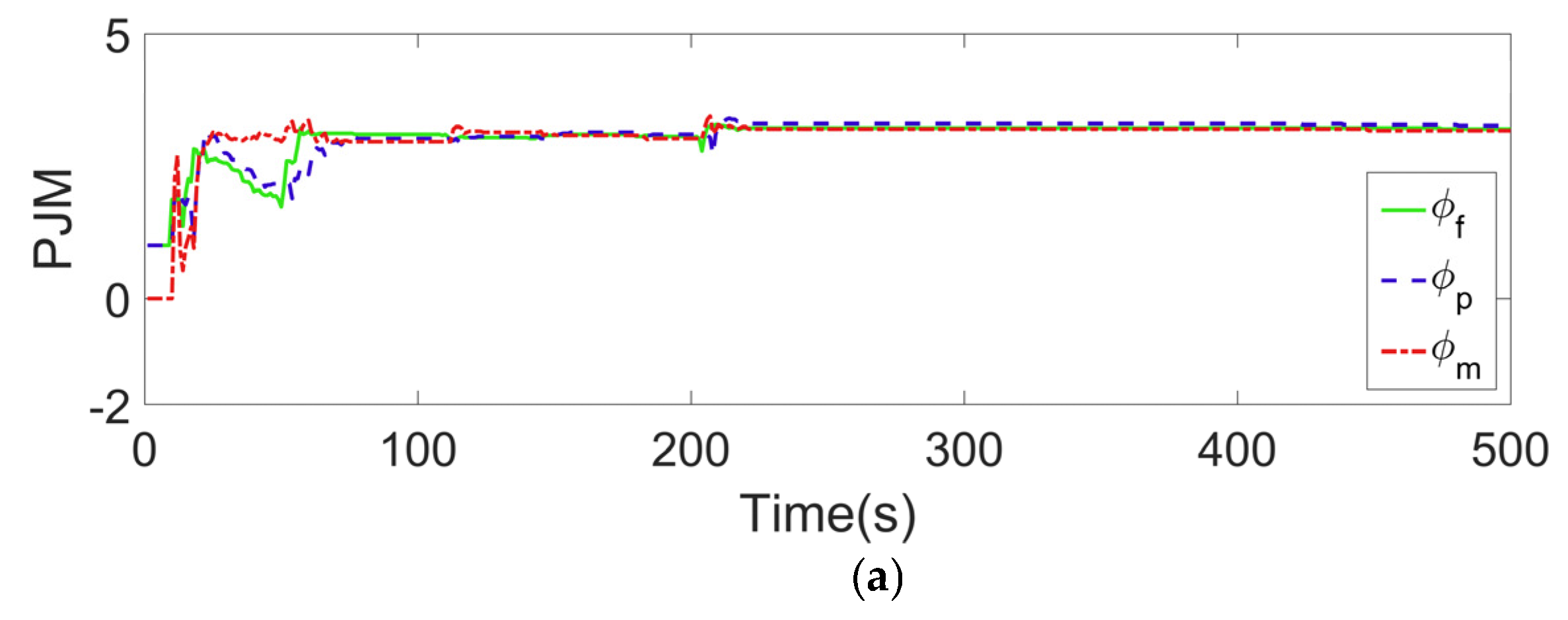
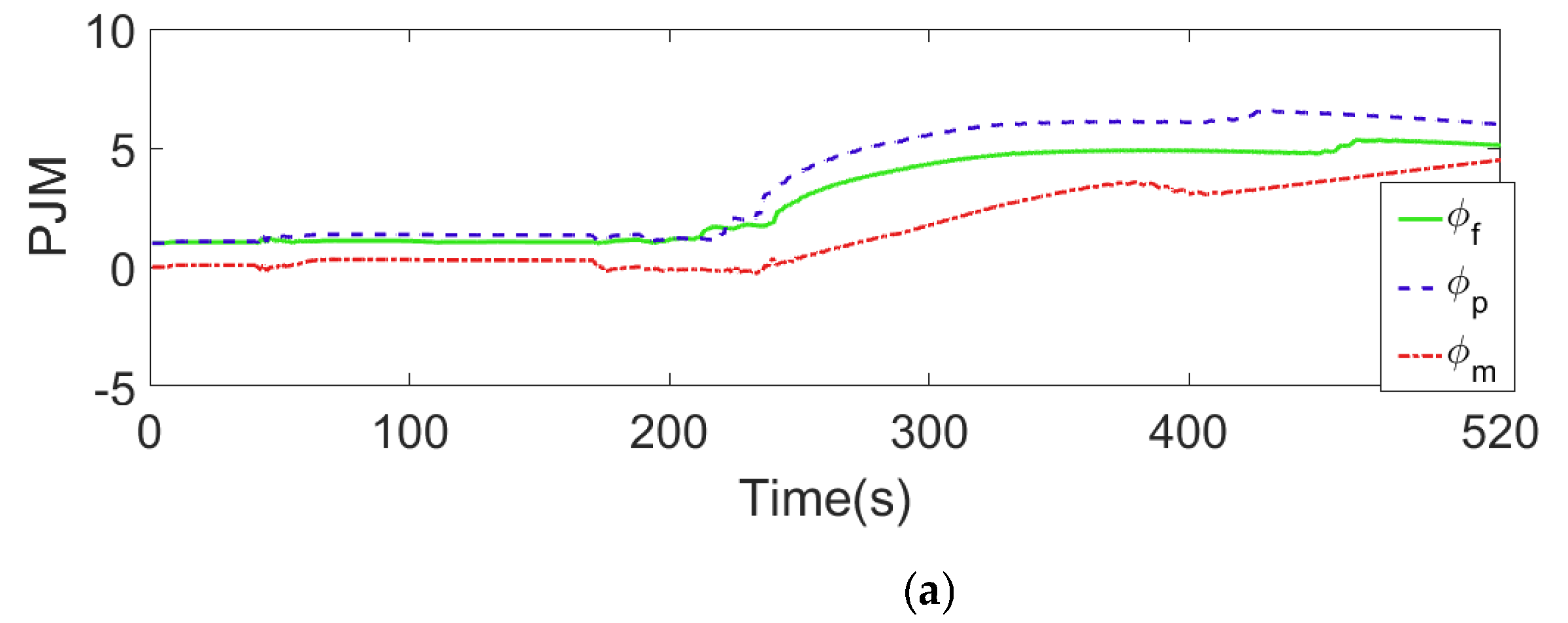
3.2. PJM Esitimation and Prediction

Since the control law contains matrixes PJM is necessary to be solved, which are time-varying matrixes. Therefore, adopting system I/O data to estimate $\Phi \left(k\right)$ and predict $\Phi \left(k+1\right),\cdots \Phi \left(k+N_u-1\right)$ is appropriate. Firstly, we estimate the PJM $\Phi \left(k\right)$.

Utilizing the projection algorithm to estimate the PJM, therefore, the criterion function of this time-varying parameter is set as follows:

$$J\left(\Phi \left(k\right)\right)=\Vert \Delta \widehat{x}\left(k\right)-\Phi \left(k\right)\Delta u\left(k-1\right)-{\widehat{f}}_d\left(k-1\right){\Vert }^2+\mu \Vert \Phi \left(k\right)-\widehat{\Phi }\left(k-1\right){\Vert }^2$$

(16)

By using the optimal solution $\partial J/\partial \widehat{\Phi }\left(k\right)$, we can obtain:

$$\widehat{\Phi }\left(k\right)=\widehat{\Phi }\left(k-1\right)+\frac{\zeta \left[\Delta \widehat{x}\left(k\right)-\Phi \left(k\right)\Delta u\left(k-1\right)-{\widehat{f}}_d\left(k-1\right)\right]\Delta u^T\left(k-1\right)}{\mu +\Vert \Delta u\left(k-1\right){\Vert }^2}$$

(17)

In order to make the estimation algorithm possess higher time-varying tracking ability, the reset algorithm is set as follows:

Set ${\widehat{\phi }}_{ii}\left(k\right)={\widehat{\phi }}_{ii}\left(1\right)$, if $\left|{\widehat{\phi }}_{ii}\left(k\right)\right|\le {\beta }_1$ or $\left|{\widehat{\phi }}_{ii}\left(k\right)\right|\ge \alpha {\beta }_1$ or $sign\left({\widehat{\phi }}_{ii}\left(1\right)\right)\ne sign\left({\widehat{\phi }}_{ii}\left(k\right)\right)$, $i=1,\cdots ,m$.

Set ${\widehat{\phi }}_{ij}\left(k\right)={\widehat{\phi }}_{ij}\left(1\right)$, if $\left|{\widehat{\phi }}_{ij}\left(k\right)\right|\ge {\beta }_2$ or $sign\left({\widehat{\phi }}_{ij}\left(1\right)\right)\ne sign\left({\widehat{\phi }}_{ij}\left(k\right)\right),$ $i,j=1,\cdots ,m$, $i\ne j$. where:$\mu$ is the penalty factor, $\mu >0$, $\zeta \in \left(0,2\right]$ is the step factor, which makes the algorithm more general, ${\beta }_1,{\beta }_2$ and $\mathsf{\alpha }$ are small enough positive constants.

Since $\mathrm{k}+1$ and subsequent moments cannot be estimated from I/O data directly, we applied the prediction algorithm to calculate these estimated PJM. Adopting multi-layer progressively increase order, utilizing historical data $\widehat{\Phi }\left(1\right)\cdots \widehat{\Phi }\left(k\right)$ to make predictions the estimated values of PJM subsequent moments. It has the property of constantly updating parameters, resulting in a small prediction error.

Based on the estimation algorithm (17), we can obtain a range of estimate values: $\widehat{\Phi }\left(1\right), \cdots , \widehat{\Phi }\left(k\right)$, then utilize these estimate values to build an auto-regressive (AR) model that can be relied on to design a prediction algorithm:

$$\widehat{\Phi }\left(k+j\right)={\displaystyle \sum }_{j=1}^{N_u-1}{\displaystyle \sum }_{i=1}^{n_p}{\xi }_i\left(k\right)\widehat{\Phi }\left(k-i+j\right)$$

(18)

Consider the criterion function as follows:

$$J\left(\xi \left(k\right)\right)=\Vert \widehat{\Phi }\left(k\right)-{\widehat{\Phi }}_t\left(k-1\right)\xi \left(k\right){\Vert }^2+\delta \Vert \xi \left(k\right)-\widehat{\xi }\left(k-1\right){\Vert }^2$$

(19)

By using the optimal solution $\partial J/\partial \widehat{\xi }\left(k\right)=0$, we can obtain:

$$\xi \left(k\right)=\xi \left(k-1\right)+\frac{{\widehat{\Phi }}_t\left(k-1\right)\left[\widehat{\Phi }\left(k\right)-{\widehat{\Phi }}_t^T\left(k-1\right)\xi \left(k-1\right)-{\widehat{f}}_d\left(k+1\right)\right]}{\delta +\Vert {\widehat{\Phi }}_t\left(k-1\right){\Vert }^2}$$

(20)

Defining the reset algorithm as:

Set ${\widehat{\phi }}_{ii}\left(k\right)={\widehat{\phi }}_{ii}\left(1\right)$, if $\left|{\widehat{\phi }}_{ii}\left(k\right)\right|\le {\beta }_1$ or $\left|{\widehat{\phi }}_{ii}\left(k\right)\right|\ge \alpha {\beta }_1$ or $sign\left({\widehat{\phi }}_{ij}\left(1\right)\right)\ne sign\left({\widehat{\phi }}_{ij}\left(k+j\right)\right)$, $i=1,\cdots ,m$.

Set ${\widehat{\phi }}_{ij}\left(k\right)={\widehat{\phi }}_{ij}\left(1\right)$, if $\left|{\widehat{\phi }}_{ij}\left(k\right)\right|\ge {\beta }_2$ or $sign\left({\widehat{\phi }}_{ij}\left(1\right)\right)\ne sign\left({\widehat{\phi }}_{ij}\left(k+j\right)\right)$, $i,j=1,\cdots ,m$, $i\ne j$.

Where: ${\xi }_i\left(k\right)$ are model coefficients,$\xi \left(k\right)={\left[{\xi }_1\left(k\right),{\xi }_2\left(k\right),\cdots ,{\xi }_{n_p}\left(k\right)\right]}^T$. $n_p$ represents the appropriate order, ${\widehat{\Phi }}_t\left(k\right)={\left[\widehat{\Phi }\left(k\right),\cdots ,\widehat{\Phi }\left(k-n_p\right)\right]}^T$, $\delta \in \left(0,1\right]$ is a positive constant.

Remark 3. 

Referring to the research content of article [44], the value of$n_p$is usually set at 2 to 7.

3.3. MFAPC Scheme Design and Stability Analysis

In view of the three DOF linearization data model of AUV, we consider the following criterion function:

$$J={\displaystyle \sum }_{i=1}^N\Vert x_d\left(k+i\right)-\widehat{x}\left(k+i\right){\Vert }^2+\lambda {\displaystyle \sum }_{j=0}^{N_u-1}\Vert \Delta u\left(k+j\right){\Vert }^2$$

(21)

where: $\lambda$ is a weight factor that is used to limit the variation range of control input, $x_d\left(k+i\right)$ is the desired control output at moment of $\left(k+i\right)$, $i=1,\cdots ,N$.

Denote ${\left[x_d\left(k\right),\cdots ,x_d\right]}^T=X_d\left(k\right)$. In this case, we combined the criterion function (21) into equation (15), take the partial derivative with respect to $\tau \left(k\right)$ and make it equal to zero. We can obtain the control law:

$$\Delta U_{N_u}\left(k\right)={\left[{\widehat{\Xi }}_1^T\left(k\right){\widehat{\Xi }}_1\left(k\right)+\lambda I\right]}^{-1}{\widehat{\Xi }}_1^T\left(k\right)\left[X_d\left(k+1\right)-E\left(k\right)\widehat{x}\left(k\right)\right]$$

(22)

When the dimensions of the system I/O data are very large, the matrix inversion is computationally expensive. Therefore, we simplified (22) and obtained the control law as follows:

$$\Delta U_{N_u}\left(k\right)=\frac{{\widehat{\Xi }}_1^T\left(k\right)\left[X_d\left(k+1\right)-E\left(k\right)\widehat{x}\left(k\right)\right]}{\lambda +\Vert {\widehat{\Xi }}_1\left(k\right){\Vert }^2}$$

(23)

where:

$${\widehat{\Xi }}_1\left(k\right)={\left[\begin{array}{c}\begin{array}{cccc}\widehat{\Phi }\left(k\right)& 0& & \cdots 0\\ \widehat{\Phi }\left(k\right)& \widehat{\Phi }\left(k+1\right)& & \cdots 0\\ ⋮& ⋮& & \ddots ⋮\\ \widehat{\Phi }\left(k\right)& \widehat{\Phi }\left(k+1\right)& \cdots & \widehat{\Phi }\left(k+N_u-1\right)\\ ⋮& ⋮& \ddots & ⋮\\ \widehat{\Phi }\left(k\right)& \widehat{\Phi }\left(k+1\right)& \cdots & \widehat{\Phi }\left(k+N_u-1\right)\end{array}\end{array}\right]}_{N\times N_u}$$

Moreover, the present moment control law expresses as:

$$u\left(k\right)=u\left(k-1\right)+g^T\Delta U_{N_u}\left(k\right)$$

(24)

where:$g={\left[I_{m\times m},O_{m\times m},\cdots ,O_{m\times m}\right]}^T\in R^{m\times N_u}$, $O_{m\times m}={\left[\begin{array}{ccc}0& \cdots & 0\\ ⋮& \ddots & ⋮\\ 0& \cdots & 0\end{array}\right]}_{m\times m}$

For the proposed control algorithm, the stability of the system needs to be rigorously verified, so we introduce the following assumption and lemma.

Assumption 3. 

The PJM $\Phi \left(k\right)$of system is a diagonally-dominant matrix which satisfies the following conditions:${\beta }_1\le \left|{\phi }_{ii}\left(k\right)\right|\le \alpha {\beta }_1$,$\left|{\phi }_{ij}\left(k\right)\right|\le {\beta }_2$,${\beta }_2>{\beta }_1\left(2\alpha +1\right)\left(m-1\right)$,$\alpha \ge 1$,$i\in \left[1,m\right]$,$j\in \left[1,m\right]$,$i\ne j$, and the sign of all elements in$\Phi \left(k\right)$remain invariant.

Lemma 2. 

([45]). Let$A_g$is a n-order complex matrix,$A_g={\left({\alpha }_{ij}\right)}_{n\times n}$, for$\forall i\in \left[1,n\right]$. Defining the Gerschgotin disc as$R_i=\left\{z\left|\left|z-{\alpha }_{ii}\right|\le {\displaystyle \sum }_{j=1,j\ne i}^n\left|{\alpha }_{ij}\right|\right.\right\}$, then all characteristic roots of the matrix satisfy that$z_i\in R_A=\underset{i=1}{\overset{n}{{\displaystyle \Delta }}}{R}_i$.

Theorem 1. 

If system (5) satisfies three assumptions which are presented previously, then when the desired signal$y_d\left(k+1\right)=y_d=const$, there must exist constant ${\lambda }_{min}>0$, and $\forall \lambda >{\lambda }_{min}$.The system satisfies the following conditions:

Tracking error sequence convergence, that is, $\underset{k\to \infty }{\lim }\widehat{x}\left(k+1\right)-x_d{\left(k\right)}_v=0$

The input $\left\{u\left(k\right)\right\}$ and output $\left\{\widehat{x}\left(k\right)\right\}$ of system are bound.

Proof. 

See Appendix A.

3.4. Fuzzy State Observer and Stability Analysis

The discrete-time fuzzy model based FSO is fit with MFAPC scheme, which is designed based on system equivalence Cauchy-discretization model. The observer can directly utilize system online I/O data. Regarding the system (6), there exists an uncertain time-delay, and we designed the FSO to deal with the unknown time-delay in the system. The number of rules and variable conditions of fuzzy observer were consistent with the fuzzy model of the controlled object. The observer of the fuzzy time-delay system is expressed as follows:

Rule i: if $z_1\left(k\right)$ is $F_{i1}$ and $z_2\left(k\right)$ is $F_{i2}$ and $\cdots$ and $z_n\left(k\right)$ is $F_{in}$, then

$$\left\{\begin{array}{c}\dot{\widehat{x}}\left(k\right)=A_{1i}\widehat{x}\left(k\right)+A_{di}\widehat{x}\left(k+d\right)+B_{i}u\left(k\right)+G_i\left(y\left(k\right)-\widehat{y}\left(k\right)\right)\\ \widehat{y}\left(k\right)=C_i\widehat{x}\left(k\right)\end{array}\right.$$

(25)

By means of the single point fuzzification, product inference, and average weighted defuzzification, the time-delay fuzzy system can be expressed as:

$$\left\{\begin{array}{c}\dot{\widehat{x}}\left(k\right)={\displaystyle \sum _{i=1}^N}{h}_i\left(z\left(k\right)\right)\left[A_{1i}\widehat{x}\left(k\right)+A_{di}\widehat{x}\left(k+d\right)+B_{i}u\left(k\right)+G_i\left(y\left(k\right)-\widehat{y}\left(k\right)\right)\right]\\ \widehat{y}\left(z\left(k\right)\right)={\displaystyle \sum _{i=1}^N}{h}_i{C}_i\widehat{x}\left(k\right)\end{array}\right.$$

(26)

Similar to the design process of the state feedback control law, the FSO output feedback control law is:

$$u\left(k\right)=-{\displaystyle \sum }_{i=1}^N{h}_i\left(z\left(k\right)\right)K_i\widehat{x}\left(k\right)$$

(27)

Defining that observation error as $e_o\left(k\right)=x\left(k\right)-\widehat{x}\left(k\right)$ and $\tilde{x}\left(k\right)=\left[\begin{array}{c}x\left(k\right)\\ e_o\left(k\right)\end{array}\right]$, then fuzzy time-delay system observation error function is expressed as:

$${\dot{e}}_o\left(k\right)={\displaystyle \sum }_{i=1}^N{\displaystyle \sum }_{j=1}^N{h}_i\left(z\left(k\right)\right)h_j\left(z\left(k\right)\right)\left[\left(A_{1i}-G_i{C}_j\right)e_o\left(k\right)+A_{di}{e}_o\left(k+d\right)\right]$$

(28)

Therefore, the fuzzy close-loop system is expressed as:

$$\dot{\tilde{x}}\left(k\right)={\displaystyle \sum }_{i=1}^N{\displaystyle \sum }_{j=1}^N{h}_i\left(z\left(k\right)\right)h_j\left(z\left(k\right)\right)\left[G_{ij}\tilde{x}\left(k\right)+M_{ij}\tilde{x}\left(k+d\right)\right]$$

(29)

where: $G_{ij}=\left[\begin{array}{cc}{A}_{1i}-B_i{K}_j& B_i{K}_j\\ 0& A_{1i}-G_i{C}_j\end{array}\right]$, $M_{ij}=\left[\begin{array}{cc}{A}_{di}& 0\\ 0& A_{di}\end{array}\right]$.

Lemma 3 

([46]). Assume matrixes $M, N\in R^{m\times n}$ are real matrixes with suitable dimensions and $P,Q\in R^{m\times n}$ are two positive definite matrixes. If these matrices satisfy matrix inequalities $M^{T}PM-Q<0$ and $N^{T}PN-Q<0$, then $M^{T}PM+N^{T}PN-2Q<0$ is valid.

Theorem 2. 

With regard to the given fuzzy discrete time-delay system (25), when there are positive definite matrixes $R_1,R_2, Q_1,Q_2$ and the matrixes $X_i, Y_i$ satisfy the following matrix inequalities:

$$\left[\begin{array}{ccc}-R_1-Q_1& 0& R_1^T{A}_{1i}{R}_i^T{B}_i\\ 0& -Q_1& R_1^T{A}_{di}^T\\ A_{1i}{R}_1-B_i{R}_i, & A_{di}{R}_1& -R_1\end{array}\right]<0$$

(30)

$$\left[\begin{array}{ccc}-R_2-Q_2& 0& {\left(R_2{A}_{di}-S_i{C}_i\right)}^T\\ 0& -Q_2& {\left(R_2{A}_{di}-S_i{C}_i\right)}^T\\ R_2{A}_{di}-Y_i{C}_i& R_2{A}_{di}-Y_i{C}_i& -R_2\end{array}\right]<0$$

(31)

$$\left[\begin{array}{ccc}-R_1-Q_1& 0& \frac{1}{2}{\widehat{X}}_{ij}^T\\ 0& -Q_1& \frac{1}{2}{\left(A_{di}{P}_1+A_{dj}{P}_1\right)}^T\\ \frac{1}{2}{\widehat{X}}_{ij}& \frac{1}{2}\left(A_{di}{R}_1+A_{dj}{R}_1\right)& -R_1\end{array}\right]<0$$

(32)

$$\left[\begin{array}{ccc}-R_1-Q_2& 0& \frac{1}{2}{\widehat{Y}}_{ij}^T\\ 0& -Q_2& \frac{1}{2}{\widehat{Y}}_{ij}^T\\ \frac{1}{2}{\widehat{Y}}_{ij}& \frac{1}{2}{\widehat{Y}}_{ij}& -R_2\end{array}\right]<0$$

(33)

then the control law (27) makes fuzzy close-loop time-delay system (28) asymptotically stable, the state feedback gain and the observed gain are $K_i=X_i{R}_1^{-1}$ and $G_i=R_2^{-1}{Y}_i$ respectively, $i\in \left[1,N\right].$

Where: ${\widehat{X}}_{ij}=A_{1i}{R}_1+A_{1j}{R}_1-B_i{X}_j-B_j{X}_i$ and ${\widehat{Y}}_{ij}=R_2{A}_{di}+R_2{A}_{dj}-Y_i{C}_j-Y_j{C}_i,$ $i<j$.

Proof. 

See Appendix B.

4. Simulation Validation

In this section, simulations were conducted to demonstrate the robustness and effectiveness of the proposed control scheme. In order to present the control performances of improved MFAPC, we designed two trajectory tracking scenarios. Simultaneously, we compared the simulation results with previous research literature about data-driven based model-free adaptive control approaches [43,47] to verify the effectiveness and feasibility.

4.1. Parameter Selection

To ensure the values of parameters possessed practicality and authenticity, we adopted realistic parameters from the AUV “T-SEA I” which was developed for underwater docking experiments. The technical specifications of the AUV have been introduced in our previous study [48], and the specific parameters are listed in

Table 1. Performance parameters of AUV “T-SEA I”.

Performance Parameter	Values
Mass(kg)	65
Length(m)	2.14
Diameter(m)	0.22
Maximum speed(kn)	2.5
Maximum depth(m)	60
Battery life(h)	6

.

For the following simulations, the parameters and system gains of the controller were set consistently [49], which are listed in

Table 2. Parameters setting for algorithms.

Performance Parameter	Values
$\mu$	1
$\zeta$	0.8
$\rho$	1
$\lambda$	0.56
d	1.2

.

As the comparative simulation control scheme, the MFAC control law is expressed as follows. Meanwhile, the comparative schemes MFAC and MFAPC do not have a specific subsystem that is used to deal with the time-delay, so the controller is unable to adopt the $\widehat{x}\left(k\right)$ as output data.

$$u\left(k\right)=u\left(k-1\right)+\frac{\rho {\widehat{\Phi }}^T\left(k\right)\left[x_d\left(k+1\right)-x\left(k\right)\right]}{\lambda +\Vert \widehat{\Phi }\left(k\right){\Vert }^2}$$

(34)

where: $\widehat{\Phi }\left(k\right)$ is estimated by (17), and the reset algorithm for $\widehat{\Phi }\left(k\right)$ is kept consistent with the proposed control scheme in Section 3.

Regarding to T-S fuzzy system, following two fuzzy rules are considered:

• Rule1: If $z_1\left(k\right)$ is $F_1$(max)
• Then $\dot{x}\left(k\right)=A_{1}x\left(k\right)+A_{d1}x\left(k-d\right)+B_{1}u\left(k\right)$
•  
• Rule2: If $z_1\left(k\right)$ is $F_2$(min)
• Then $\dot{x}\left(k\right)=A_{2}x\left(k\right)+A_{d2}x\left(k-d\right)+B_{2}u\left(k\right)$

The membership function is selected as a Gaussian normal distribution, consistent with article [50], and the matrix parameters for two modals of fuzzy systems are:

$$\begin{gathered} A_1=\left[\begin{array}{cc}-8& 0.3\\ 3& 1\end{array}\right], A_2=\left[\begin{array}{cc}-6& 0.3\\ 2& 1\end{array}\right] \\ {A}_{d1}=\left[\begin{array}{cc}0.2& -0.4\\ 0.3& 0.4\end{array}\right], A_{d2}=\left[\begin{array}{cc}0.3& -0.3\\ 0.3& 0.5\end{array}\right] \\ {B}_1=\left[\begin{array}{cc}0.1& 0.3\\ 0.3& 0.1\end{array}\right], B_2=\left[\begin{array}{cc}0.1& 0.2\\ 0.3& 0.1\end{array}\right] \\ {C}_1=C_2=\left[\begin{array}{cc}1& 0\\ 0& 1\end{array}\right]. \end{gathered}$$

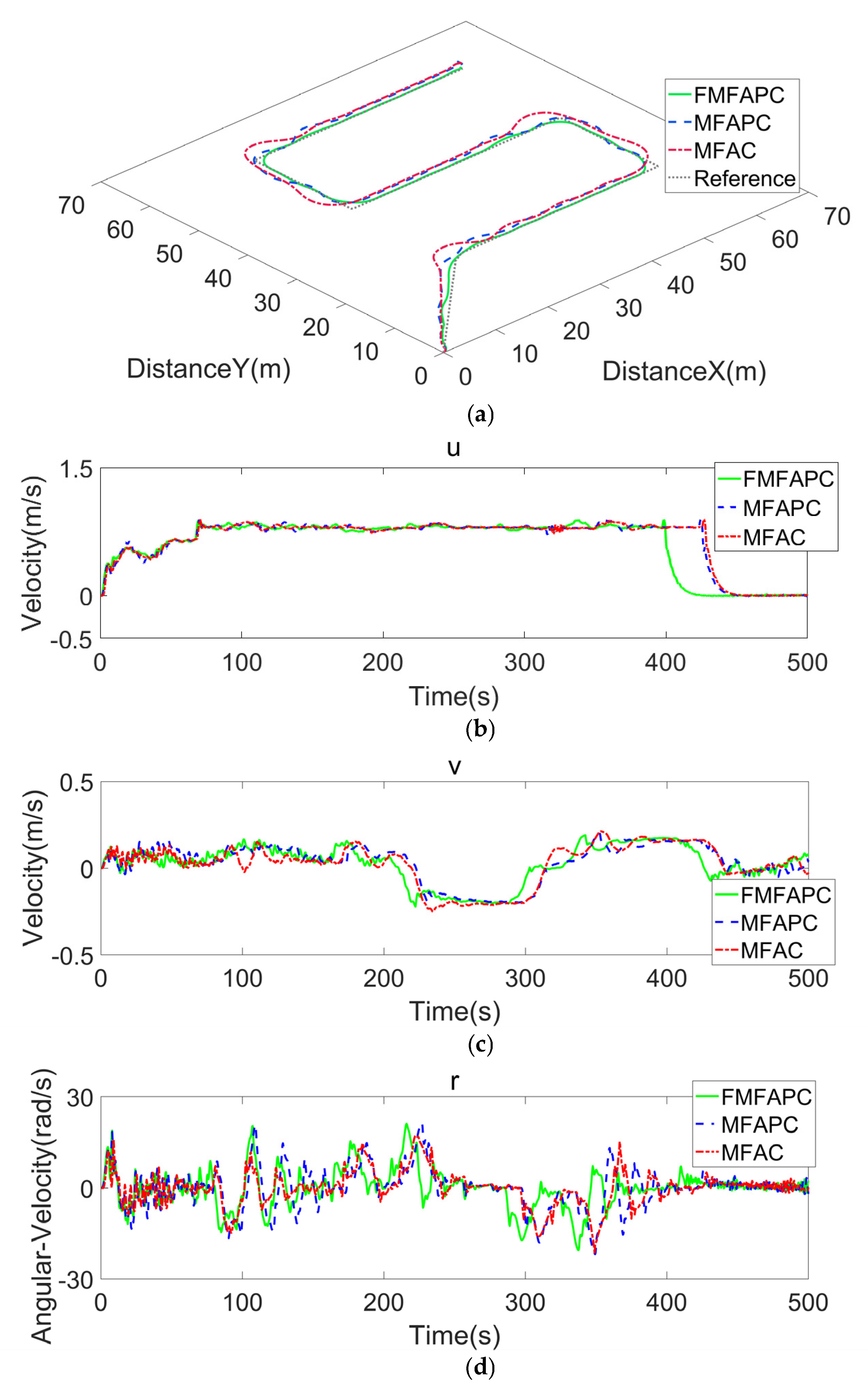
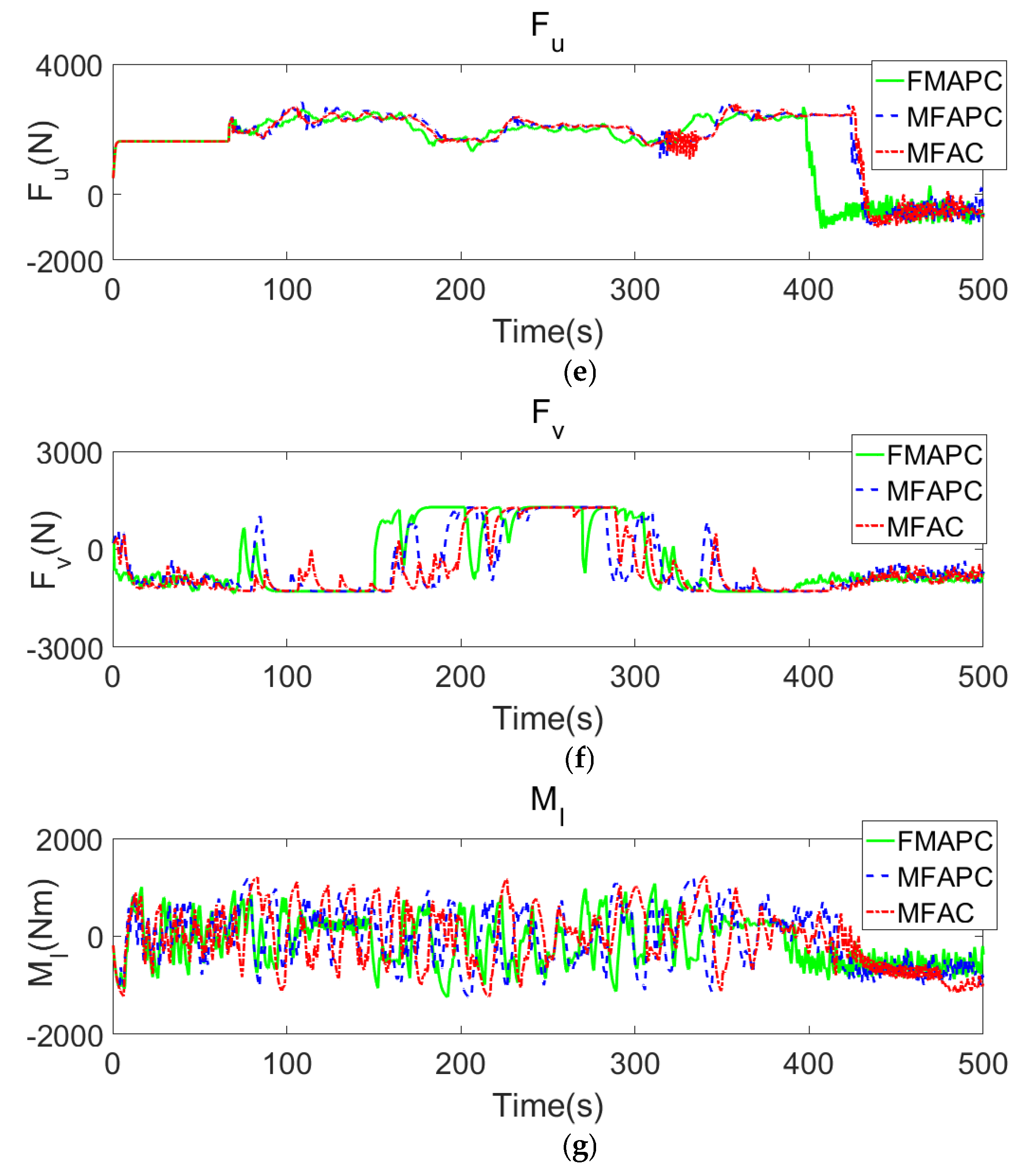
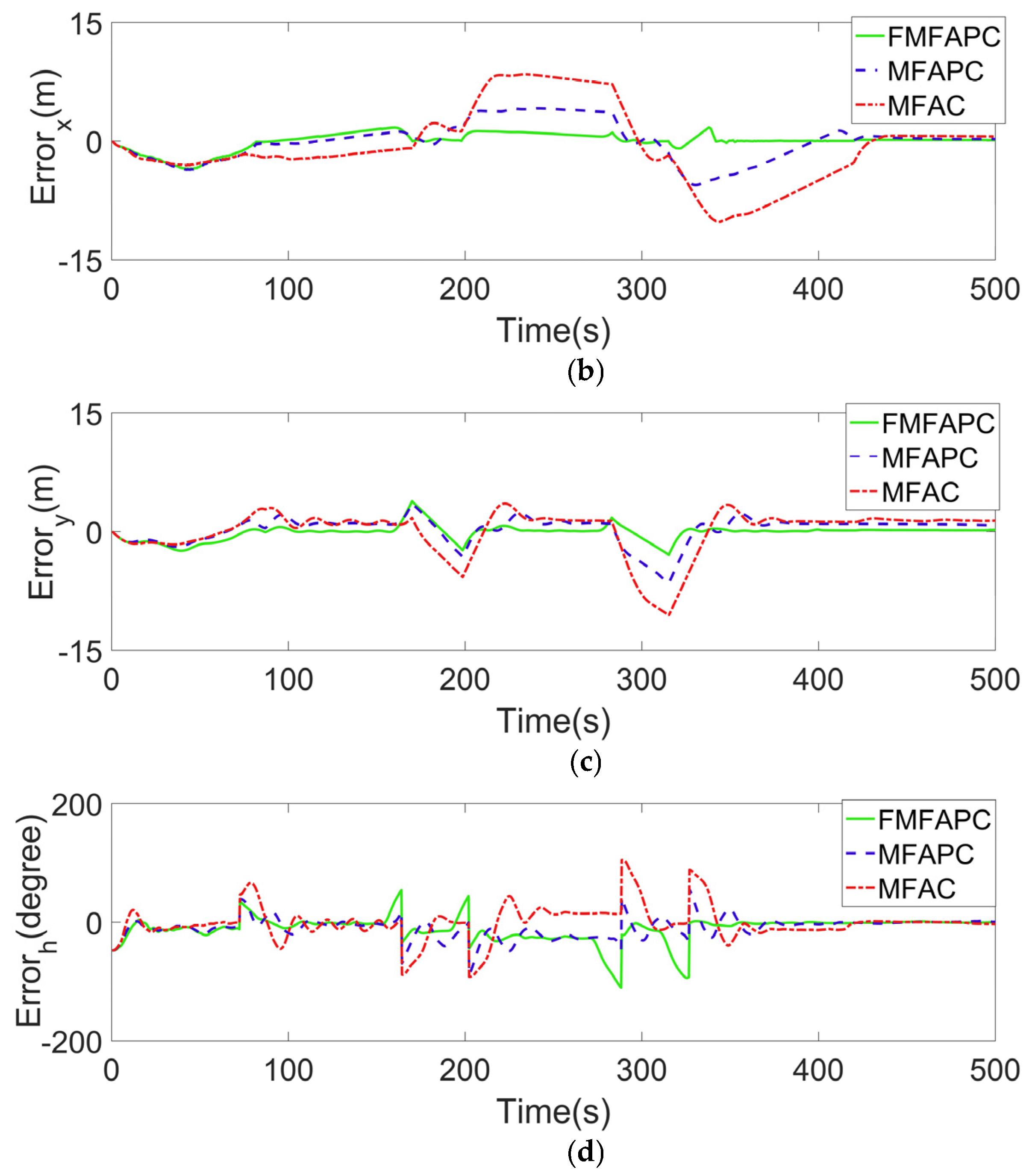
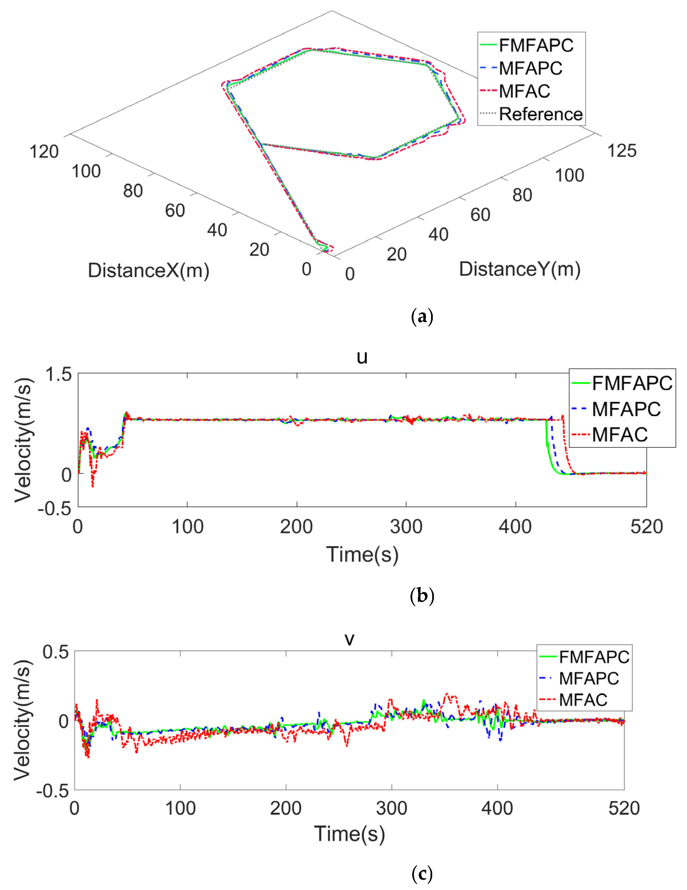
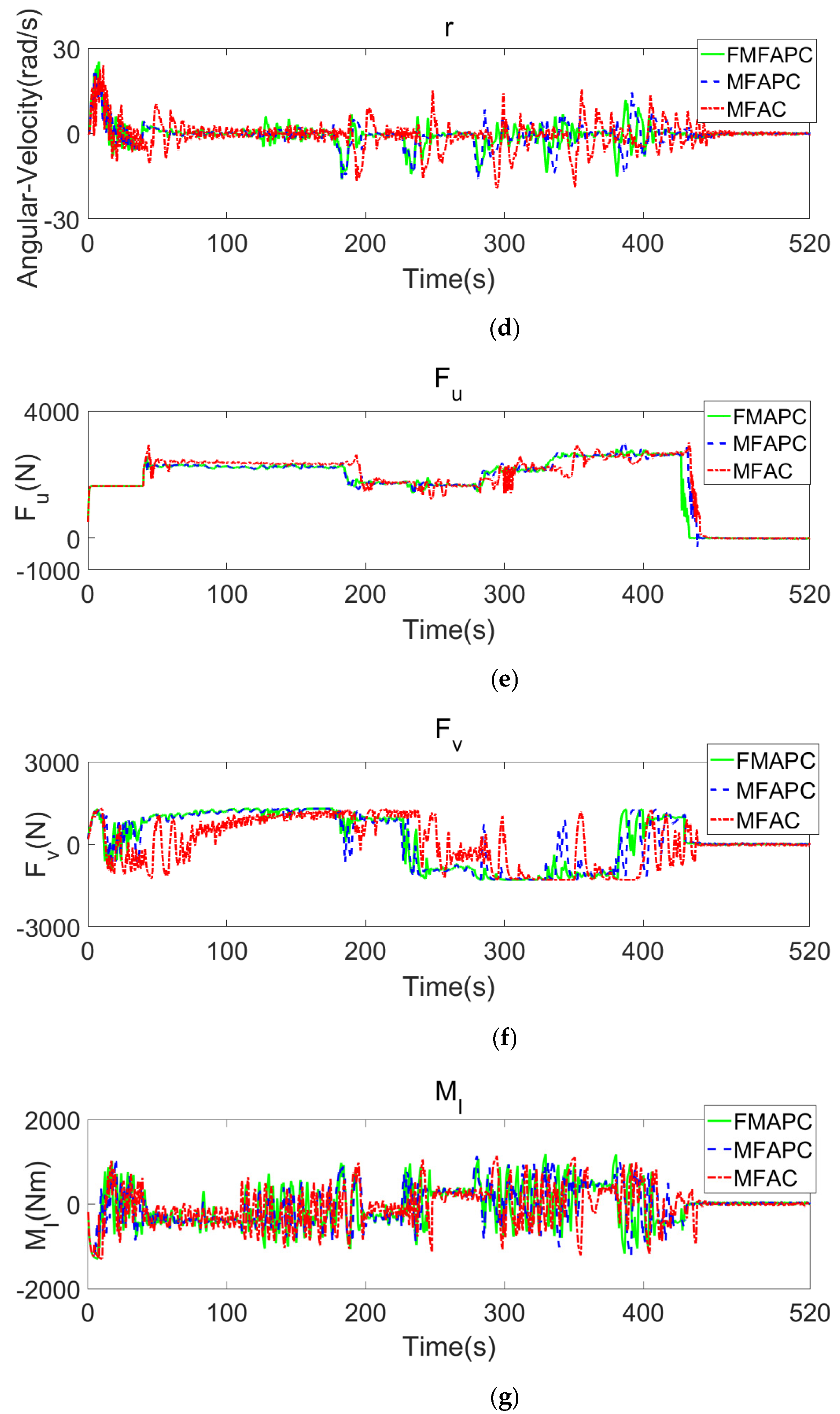
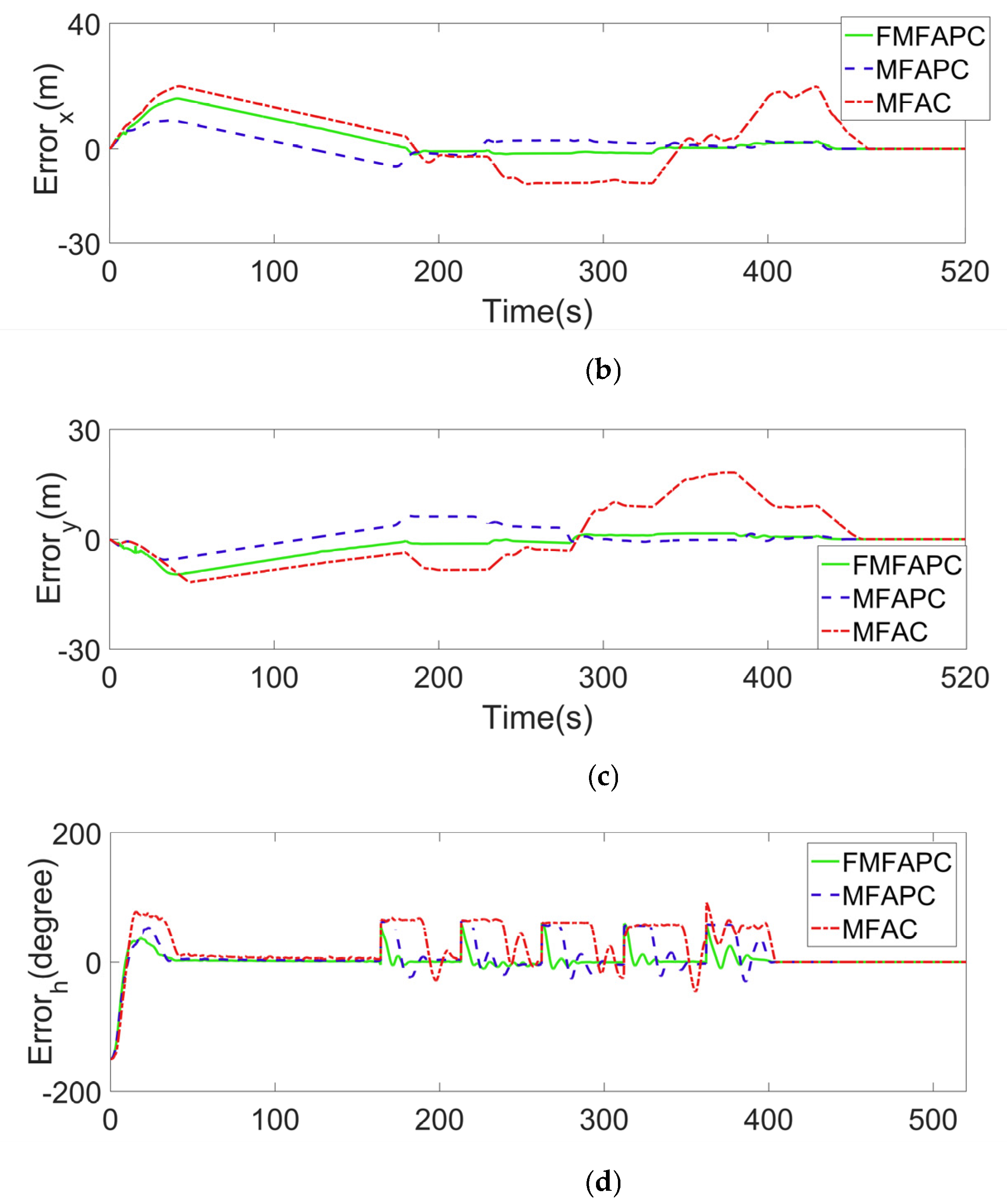
4.2. Tracking Simulation Results

In order to examine the control performance of the proposed algorithm, two trajectory tracking scenarios were designed. Considering the external disturbance from the current in an area of offshore water, the current was set at 0.2 m/s. Under these two scenarios, both initial settings were identical, the initial position and attitude are set as ${\left[x\left(0\right),y\left(0\right),\psi \left(0\right)\right]}^T={\left[0,0,0\right]}^T$, and the initial velocities are set as ${\left[u\left(0\right),v\left(0\right),r\left(0\right)\right]}^T={\left[0,0,0\right]}^T$.

To appraise the performances of the proposed controller and the contrast controllers, we choose to used standard deviation (STD) and mean absolute deviation (MAD) to calculate the practical sailing trajectories and yaw angles. The controller’s accuracy can be presented more intuitionistic and clearer. In the following value calculation, all values were listed at three decimal places.

$$\left\{\begin{array}{c}STD=\sqrt{\raisebox{1ex}{${{\displaystyle \sum }}_{i=1}^N\left(y_i-\overline{y}\right)$}\!\left/ \!\raisebox{-1ex}{$N$}\right.}\\ MAD=\raisebox{1ex}{${{\displaystyle \sum }}_{i=1}^N\left|y_i-y_d\right|$}\!\left/ \!\raisebox{-1ex}{$N$}\right.\end{array}\right.$$

(35)

4.2.1. Scenario 1

In this scenario, we designed a comb-shaped trajectory for AUV to execute tracking simulation under the synchronous influence of external disturbance and time delay. We set six reference coordinates as inflection points for AUV horizontal plane sailing, which were $\left[20,20\right]$, $\left[60,20\right]$,$\left[60,40\right]$,$\left[20,40\right]$,$\left[20,60\right],$ and $\left[60,60\right]$ serially, the current was set with disturbance parallel to the y-axis. The reference trajectory was set as follows:

$$\begin{gathered} x_d\left[m\right]=\left\{\begin{array}{c}\frac{2}{7}t, t\le 70s\\ \frac{4}{9}\left(t-70\right)+20, 70s<t\le 160s\\ 0, 160s<t\le 200s\\ 60-\frac{4}{9}\left(t-200\right), 200s<t\le 290s\\ 0, 290s<t\le 330s\\ \frac{4}{9}\left(t-330\right)+20, t>330s\end{array}\right. \\ {y}_d\left[\mathrm{m}\right]=\left\{\begin{array}{c}\frac{2}{7}t, t\le 70s\\ 0, 70s<t\le 160s\\ \frac{1}{2}\left(t-160\right)+20, 160s<t\le 200s\\ 0, 200s<t\le 290s\\ \frac{1}{2}\left(t-290\right)+40, 290s<t\le 330s\\ 0, t>330s\end{array}\right. \end{gathered}$$

The tracking results of the proposed control approach and typical MFAC and MFAPC are shown in Figure 1 and Figure 2.

By observing the tracking comparative experiment results shown in Figure 1a, it can be immediately determined that tracking performance was effectively assured via applying our proposed FSO-based MFAPC approach, and exhibits the best tracking accuracy under the synchronous influence of time-delay and external disturbance, and the superiority of tracking accuracy at all inflection corners becomes more obvious.

As seen in the control input and output details are shown in Figure 1b–g, the proposed control approach possesses a better capability of processing system time-delay than typical MFAC or MFAPC approach. The control outputs show that the proposed approach attenuates the influence of the system time-delay while the error of the contrast controller gradually increases.

When combined with the predictive control concept, the MFAPC can predict the dynamic changes of the system in a certain future time window via the PJM predictive technique, allowing it to deal with external disturbances better than the traditional MFAC approach. For the PJM values shown in Figure 2a, we can see that during the first 70 time points, the proposed algorithm and typical MFAPC can both dynamically change related to the system dynamic variation, but the PJM of the proposed algorithm has smaller overshot and faster convergence. In addition, the corresponding controllers’ performances are listed in

Table 3. STD and MAD of controllers under Scenario 1.

Controller	STDx(m)	MADx(m)	STDy(m)	MADy(m)	STDyaw(°)	MADyaw(°)
FMFAPC	19.356	1.094	20.066	0.556	24.373	11.225
MFAPC	19.733	1.791	20.154	1.449	25.043	12.613
MFAC	19.992	3.406	20.108	1.985	30.327	15.74

. From comparing the STD values and MAD values, we can conclude that the proposed controller has the smallest overshoot and the best tracking accuracy.

4.2.2. Scenario 2

In this scenario, we designed a hexagon trajectory, the tracking simulation under the synchronous influence of external disturbance and time delay. We set six reference coordinates as AUV horizontal sailing inflection points, which were [105,60], [105,100], [70,120], [35,100], [35,60], and [70,40] serially, the current disturbances were both set parallel to the x-axis and y-axis as 0.2 m/s. The reference trajectory was set as follows:

$$\begin{gathered} x_d\left[m\right]=\left\{\begin{array}{c}\frac{21}{32}t, t\le 160s\\ 0, 160s<t\le 210s\\ 105-\frac{7}{10}\left(t-210\right), 210s<t\le 310s\\ 0, 310s<t\le 360s\\ 35+\frac{7}{10}\left(t-360\right), t>360s\end{array}\right. \\ {y}_d\left[m\right]=\left\{\begin{array}{c}\frac{3}{8}t, t\le 160s\\ \frac{4}{5}\left(t-160\right)+60, 160s<t\le 210s\\ \frac{2}{5}\left(t-210\right)+100, 210s<t\le 260s\\ 120-\frac{2}{5}\left(t-260\right), 260s<t\le 310s\\ 100-\frac{4}{5}\left(t-310\right), 310s<t\le 360s\\ 60-\frac{2}{5}\left(t-360\right), t>360s\end{array}\right. \end{gathered}$$

The tracking results of the proposed control approach and typical MFAC and MFAPC are presented in Figure 3 and Figure 4.

From the simulation results in Figure 3a, we can also intuitively find that by adopting an FSO based MFAPC algorithm, the accuracy of tracking control was relatively well guaranteed. Meanwhile, the proposed control approach can ensure rapid convergence to the reference trajectory with much smaller course slips and deviations. Meanwhile, it can be found that the proposed control approach possesses a faster convergence rate from the simulation results presented in Figure 3b−g under the influence of system time-delay and external disturbance.

The simulation results presented in Figure 4a indicate that the proposed FSO based MFAPC can respond to the system’s dynamic variation to change the PJM estimation and prediction value with a faster response time and a faster convergence rate, indicating that the proposed control approach has better robustness and adaptiveness. The corresponding controllers’ performances under this scenario are listed in

Table 4. STD and MAD of controllers under Scenario 2.

Controller	STDx(m)	MADx(m)	STDy(m)	MADy(m)	STDyaw(°)	MADyaw(°)
FMFAPC	26.461	2.850	31.150	2.213	45.020	6.242
MFAPC	26.024	3.133	31.418	2.520	45.551	14.403
MFAC	28.509	3.213	33.049	7.965	48.557	27.807

, the STD values and MAD values reflect the superiority of the proposed control approach, which possesses relatively best accuracy and smallest control overshoot.

In summary, the proposed FSO based MFAPC algorithm possesses strong robustness towards system synchronous influence time-delay and external disturbance, the proposed algorithm achieves good performance in estimating the system parameter uncertainty, and the control scheme is able to achieve satisfactory tracking accuracy and convergence rate.

Remark 4 

The proposed FSO based MFAPC scheme is designed based on the data-driven concept and dynamic linearization technique, it relays on I/O data to generate controllers directly. Thus, the accuracy of I/O data measurement directly affects the performance of the control scheme. In practical applications, the system noises, performance of sensors, data packet loss, transmission rate of network channel, etc., these factors will deteriorate the controller performance.

5. Conclusions

In this study, a fuzzy state observer based MFAPC scheme is proposed for trajectory tracking control for AUV. We First time combining the state observer based on fuzzy logic concept with data-driven control approach. Considering the practical characteristics of the AUVs motion system, the dynamic linearization method of proposed control approach was designed able to process MIMO discrete-time system. Meanwhile, the discrete-time fuzzy model based FSO fits with MFAPC scheme, which is designed based on system equivalence Cauchy-discretization model. The observer can directly utilize system online I/O data. To verifying the proposed control scheme of this study, we compared the control performances of proposed algorithm with typical MFAC and MFAPC approaches. We adopted parameters values of practical AUV as controller parameters. We design two different tracking scenarios, and set external disturbances to simulate ocean environment of off shore water. Depend on these simulation conditions, the simulation were conducted by using MATLAB/Simulink.

From an implementation perspective, the proposed control scheme is an effective and attractive approach. Firstly, it does not require precise parameters or an accurate mathematical model to generate controller data, which is replaced by online I/O data. Secondly, compared with a typical MFAC or other data-driven based approach, the proposed control scheme has the capability of synchronous compensation of the time-delay and external disturbance and can exhibit tracking the performance of high robustness and accuracy. Last but not least, our proposed control scheme can be applied to other kinds of robotic systems and even multi-agent systems.

The proposed control approach has satisfactory performance in the working environments with unknown or uncertain hydrodynamics. However, aim to the operation conditions such as extremely high time accuracy requirement, high sailing-speed vehicles or object system mode will random jump, the algorithm of this study cannot achieve highly robustness or accuracy. As future research, these limitations of proposed algorithm are worth to devote efforts.

References

1. Palomeras, N.; Vallicrosa, G.; Mallios, A.; Bosch, J.; Vidal, E.; Hurtos, N.; Carreras, M.; Ridao, P. AUV homing and docking for remote operations. Ocean Eng. 2018, 154, 106–120. [Google Scholar] [CrossRef]
2. Hadi, B.; Khosravi, A.; Sarhadi, P. A review of the path planning and formation control for multiple autonomous underwater vehicles. J. Intell. Robot. Syst. 2021, 101, 67. [Google Scholar] [CrossRef]
3. Kamaev, A.N.; Sukhenko, V.A.; Karmanov, D.A. Constructing and visualizing three-dimensional sea bottom models to test AUV machine vision systems. Program. Comput. Softw. 2017, 43, 184–195. [Google Scholar] [CrossRef]
4. Tonacci, A.; Lacava, G.; Lippa, M.A.; Lupi, L.; Cocco, M.; Domenici, C. Electronic nose and AUV: A novel perspective in marine pollution monitoring. Mar. Technol. Soc. J. 2015, 49, 18–24. [Google Scholar] [CrossRef]
5. Cao, X.; Sun, H.; Guo, L. Potential field hierarchical reinforcement learning approach for target search by multi-AUV in 3-D underwater environments. Int. J. Control. 2020, 93, 1677–1683. [Google Scholar] [CrossRef]
6. Gan, W.; Zhu, D.; Xu, W.; Sun, B. Survey of trajectory tracking control of autonomous underwater vehicles. J. Mar. Sci. Technol. 2017, 25, 722–731. [Google Scholar]
7. Lu, L.; Wang, D.; Peng, Z.; Wang, H. Predictor-based los guidance law for path following of underactuated marine surface vehicles with sideslip compensation. Ocean Eng. 2016, 124, 340–348. [Google Scholar] [CrossRef]
8. Elmokadem, T.; Zribi, M.; Youcef-Toumi, K. Terminal sliding mode control for the trajectory tracking of under actuated autonomous underwater vehicles. Ocean. Eng. 2017, 129, 613–625. [Google Scholar] [CrossRef]
9. Cho, G.R.; Li, J.H.; Park, D.; Jung, J.H. Robust trajectory tracking of autonomous underwater vehicles using back-stepping control and time delay estimation. Ocean. Eng. 2020, 201, 107131. [Google Scholar] [CrossRef]
10. Avila, J.P.; Donha, D.C.; Adamowski, J.C. Experimental model identification of open-frame underwater vehicles. Ocean. Eng. 2013, 60, 81–94. [Google Scholar]
11. Caccia, M.; Indiveri, G.; Veruggio, G. Modeling and identifification of open-frame variable confifiguration unmanned underwater vehicles. Ocean. Eng. 2000, 25, 227–240. [Google Scholar] [CrossRef]
12. Hou, Z.; Jin, S. A novel data-driven control approach for a class of discrete-time nonlinear systems. IEEE Trans. Control. Syst. Technol. 2010, 19, 1549–1558. [Google Scholar] [CrossRef]
13. Hou, Z.; Jin, S. Data-driven model-free adaptive control for a class of MIMO nonlinear discrete-time systems. IEEE Trans. Neural Networks 2011, 22, 2173–2188. [Google Scholar]
14. Hou, Z.S.; Wang, Z. From model-based control to data-driven control: Survey, classification and perspective. Inf. Sci. 2013, 235, 3–35. [Google Scholar] [CrossRef]
15. Liao, Y.; Du, T.; Jiang, Q. Model-free adaptive control method with variable forgetting factor for unmanned surface vehicle control. Appl. Ocean. Res. 2019, 93, 101945. [Google Scholar] [CrossRef]
16. Jiang, Y.; Xu, X.; Zhang, L. Heading tracking of 6WID/4WIS unmanned ground vehicles with variable wheelbase based on model free adaptive control. Mech. Syst. Signal Process. 2021, 159, 107715. [Google Scholar] [CrossRef]
17. Gao, H.; Ma, G.; Lv, Y.; Guo, Y. Forecasting-based data-driven model-free adaptive sliding mode attitude control of combined spacecraft. Aerosp. Sci. Technol. 2019, 86, 364–374. [Google Scholar] [CrossRef]
18. Hou, Z.; Chi, R.; Gao, H. An overview of dynamic-linearization-based data-driven control and applications. IEEE Trans. Ind. Electron. 2016, 64, 4076–4090. [Google Scholar] [CrossRef]
19. Hua, C.; Liu, G.; Li, L.; Guan, X. Adaptive fuzzy prescribed performance control for nonlinear switched time-delay systems with unmodeled dynamics. IEEE Trans. Fuzzy Syst. 2017, 26, 1934–1945. [Google Scholar] [CrossRef]
20. Zhang, J.X.; Yang, G.H. Fuzzy adaptive fault-tolerant control of unknown nonlinear systems with time-varying structure. IEEE Trans. Fuzzy Syst. 2019, 27, 1904–1916. [Google Scholar] [CrossRef]
21. Jiang, B.; Karimi, H.R.; Kao, Y.; Gao, C. Adaptive Control of Nonlinear Semi-Markovian Jump TS Fuzzy Systems With Immeasurable Premise Variables via Sliding Mode Observer. IEEE Trans. Cybern. 2018, 50, 810–820. [Google Scholar] [CrossRef] [Green Version]
22. Cao, Y.Y.; Frank, P.M. Analysis and synthesis of nonlinear time-delay systems via fuzzy control approach. IEEE Trans. Fuzzy Syst. 2000, 8, 200–211. [Google Scholar]
23. Hua, C.; Wang, Q.G.; Guan, X. Robust adaptive controller design for nonlinear time-delay systems via T–S fuzzy approach. IEEE Trans. Fuzzy Syst. 2018, 17, 901–910. [Google Scholar]
24. Huang, Y.; Zhang, Y.; Pool, D.M.; Stroosma, O.; Chu, Q. Time-Delay Margin and Robustness of Incremental Nonlinear Dynamic Inversion Control. J. Guid. Control. Dyn. 2022, 45, 394–404. [Google Scholar] [CrossRef]
25. Warminski, J. Nonlinear dynamics of self-, parametric, and externally excited oscillator with time delay: Van der Pol versus Rayleigh models. Nonlinear Dyn. 2020, 99, 35–56. [Google Scholar] [CrossRef]
26. Liu, X.; Xiao, J.-W.; Chen, D.; Wang, Y.-W. Dynamic consensus of nonlinear time-delay multi-agent systems with input saturation: An impulsive control algorithm. Nonlinear Dyn. 2019, 97, 1699–1710. [Google Scholar] [CrossRef]
27. Zare, I.; Setoodeh, P.; Asemani, M.H. TS fuzzy tracking control of nonlinear constrained time-delay systems using a reference-management approach. J. Frankl. Inst. 2021, 358, 9510–9541. [Google Scholar] [CrossRef]
28. Xu, S.; Sun, G.; Sun, W. Takagi–Sugeno fuzzy model based robust dissipative control for uncertain flexible spacecraft with saturated time-delay input. ISA Trans. 2017, 66, 105–121. [Google Scholar] [CrossRef] [PubMed]
29. Zhong, Z.; Zhu, Y.; Ahn, C.K. Reachable set estimation for Takagi-Sugeno fuzzy systems against unknown output delays with application to tracking control of AUVs. ISA Trans. 2018, 78, 31–38. [Google Scholar] [CrossRef] [PubMed]
30. Fossen, T.I. Handbook of Marine Craft Hydrodynamics and Motion Control; John Wiley & Sons: New York, NY, USA, 2011. [Google Scholar]
31. Healey, A.J.; Lienard, D. Multivariable sliding mode control for autonomous diving and steering of unmanned underwater vehicles. IEEE J. Ocean. Eng. 1993, 18, 327–339. [Google Scholar] [CrossRef] [Green Version]
32. Lekkas, A.M.; Fossen, T.I. Line-of-sight guidance for path following of marine vehicles. Adv. Mar. Robot. 2013, 5, 63–92. [Google Scholar]
33. Fossen, T.I.; Pettersen, K.Y.; Galeazzi, R. Line-of-sight path following for dubins paths with adaptive sideslip compensation of drift forces. IEEE Trans. Control. Syst. Technol. 2014, 23, 820–827. [Google Scholar] [CrossRef] [Green Version]
34. Fossen, T.I.; Lekkas, A.M. Direct and indirect adaptive integral line-of-sight path-following controllers for marine craft exposed to ocean currents. Int. J. Adapt. Control. Signal Process. 2017, 31, 445–463. [Google Scholar] [CrossRef]
35. Weng, Y.; Gao, X. Data-driven robust output tracking control for gas collector pressure system of coke ovens. IEEE Trans. Ind. Electron. 2016, 64, 4187–4198. [Google Scholar] [CrossRef]
36. Lei, T.; Hou, Z.; Ren, Y. Data-driven model free adaptive perimeter control for multi-region urban traffic networks with route choice. IEEE Trans. Intell. Transp. Syst. 2019, 21, 2894–2905. [Google Scholar] [CrossRef]
37. Yang, J.; Su, J.; Li, S.; Yu, X. High-order mismatched disturbance compensation for motion control systems via a continuous dynamic sliding-mode approach. IEEE Trans. Ind. Inform. 2013, 10, 604–614. [Google Scholar] [CrossRef]
38. Wang, H.O.; Tanaka, K.; Griffin, M.F. An approach to fuzzy control of nonlinear systems: Stability and design issues. IEEE Trans. Fuzzy Syst. 1996, 4, 14–23. [Google Scholar] [CrossRef]
39. Peng, F.; Wang, Y.; Xuan, H.; Nguyen, T.V.T. Efficient road traffic anti-collision warning system based on fuzzy nonlinear programming. Int. J. Syst. Assur. Eng. Manag. 2022, 13, 456–461. [Google Scholar] [CrossRef]
40. Wang, L.X. Adaptive Fuzzy System and Control: Design and Stability Analysis; Prentice-Hall Inc.: Englewood Cliffs, NJ, USA, 1994. [Google Scholar]
41. Gao, H.; Liu, X.; Lam, J. Stability analysis and stabilization for discrete-time fuzzy systems with time-varying delay. IEEE Trans. Syst. Man Cybern. Part B 2008, 39, 306–317. [Google Scholar]
42. Yu, Q.; Hou, Z. Data-driven predictive iterative learning control for a class of multiple-input and multiple-output nonlinear systems. Trans. Inst. Meas. Control. 2016, 38, 266–281. [Google Scholar] [CrossRef]
43. Hou, Z.; Jin, S. Model Free Adaptive Control; CRC Press: Boca Raton, FL, USA, 2013. [Google Scholar]
44. Han, Z. On the identification of time-varying parameters in dynamic systems. Acta Autom. Sin. 1984, 10, 330–337. [Google Scholar]
45. Hou, Z.; Jin, S. Model Free Adaptive Control: Theory and Application; Science Press: Beijing, China, 2014. [Google Scholar]
46. Gershgorin, S.A. Uber die abgrenzung der eigenwerte einer matrix. Известия Рoссийскoй академии наук. Серия Математическая 1931, 6, 749–754. [Google Scholar]
47. Boyd, S.; El Ghaoui, L.; Feron, E.; Balakrishnan, V. Linear matrix inequalities in system and control theory. Soc. Ind. Appl. Math. 1994, 15, 157–193. [Google Scholar]
48. Wu, C.; Dai, Y.; Shan, L.; Zhu, Z.; Wu, Z. Data-driven trajectory tracking control for autonomous underwater vehicle based on iterative extended state observer. Math. Biosci. Eng. 2022, 19, 3036–3055. [Google Scholar] [CrossRef] [PubMed]
49. Guo, Y.; Hou, Z.; Liu, S.; Jin, S. Data-driven model-free adaptive predictive control for a class of MIMO nonlinear discrete-time systems with stability analysis. IEEE Access 2019, 7, 102852–102866. [Google Scholar] [CrossRef]
50. Song, X.; Xu, S.; Shen, H. Robust H∞ control for uncertain fuzzy systems with distributed delays via output feedback controllers. Inf. Sci. 2008, 178, 4341–4356. [Google Scholar] [CrossRef]
51. Strang, G. Linear Algebra and Its Applications; Thomson, Brooks/Cole: Belmont, CA, USA, 2006. [Google Scholar]
Figure 1. Simulation results of scenario 1. (a) Tracking results of comb-shaped trajectory. (bd) Control outputs. (eg) Control inputs.
Jmse 11 00207 g001aJmse 11 00207 g001b
Figure 2. (a) PJM estimation results of controllers. (bd) Tracking errors.
Jmse 11 00207 g002aJmse 11 00207 g002b
Figure 3. Simulation results of scenario 2. (a) Tracking results of comb-shaped trajectory. (bd) Control outputs. (eg) Control inputs.
Jmse 11 00207 g003aJmse 11 00207 g003b
Figure 4. (a) PJM estimation results of controllers. (bd) Tracking errors.
Jmse 11 00207 g004aJmse 11 00207 g004b