
Autonomous Underwater Vehicle Based Chemical Plume Tracing via Deep Reinforcement Learning Methods

1
Electrical Engineering Department, Louisiana Tech University, Ruston, LA 71272, USA
2
Department of Electrical Engineering and Computer Science, Embry-Riddle Aeronautical University, Daytona Beach, FL 32114, USA
*
Author to whom correspondence should be addressed.
J. Mar. Sci. Eng. 2023, 11(2), 366; https://0-doi-org.brum.beds.ac.uk/10.3390/jmse11020366
Submission received: 10 January 2023
/
Revised: 23 January 2023
/
Accepted: 30 January 2023
/
Published: 6 February 2023
(This article belongs to the Special Issue Autonomous Underwater Vehicle Technology Advances in Ocean Observation)
Abstract
:This article presents two new chemical plume tracing (CPT) algorithms for using on autonomous underwater vehicles (AUVs) to locate hydrothermal vents. We aim to design effective CPT navigation algorithms that direct AUVs to trace emitted hydrothermal plumes to the hydrothermal vent. Traditional CPT algorithms can be grouped into two categories, including bio-inspired and engineering-based methods, but they are limited by either search inefficiency in turbulent flow environments or high computational costs. To approach this problem, we design a new CPT algorithm by fusing traditional CPT methods. Specifically, two deep reinforcement learning (RL) algorithms, including double deep Q-network (DDQN) and deep deterministic policy gradient (DDPG), are employed to train a customized deep neural network that dynamically combines two traditional CPT algorithms during the search process. Simulation experiments show that both DDQN- and DDPG-based CPT algorithms achieve a high success rate (>90%) in either laminar or turbulent flow environments. Moreover, compared to traditional moth-inspired method, the averaged search time is improved by 67% for the DDQN- and 44% for the DDPG-based CPT algorithms in turbulent flow environments.
1. Introduction
Autonomous underwater vehicles (AUVs) play a significant role in marine science surveys. One important application is using AUVs to find underwater hydrothermal vents. Hydrothermal vents, i.e., ocean volcanoes, are natural plumbing systems that transport heat and minerals from the interior of the Earth to the ocean [1]. Studying hydrothermal vents can help scientists investigate the origin and evolution of life on Earth [2]. Tracing the emitted hydrothermal plumes to find hydrothermal vents is the most effective method since the emitted chemical materials are distinct from the surrounding seawater and can disperse over a long distance driven by ocean currents [3]. Therefore, it is possible to deploy an AUV equipped with chemical sensors to detect emitted chemical plumes and trace them back to the source. Several successful AUV-based hydrothermal vent surveys were conducted in the Pacific [4] and Atlantic Oceans [5], which verified the feasibility of using AUVs in finding hydrothermal vents in real-world environments. However, existing AUV-based hydrothermal vent localization methods relied on a simple and fixed search trajectory, e.g., the lawn mower trajectory. Designing an effective, efficient, and intelligent hydrothermal vent search strategy requires further investigation.
The key to successfully finding hydrothermal vents is the design of an effective chemical plume tracing (CPT) algorithm [6]. CPT algorithms guide the search agent, i.e., an AUV, to detect chemical plumes as cues to find the source. A similar application is image-based navigation [7], which directs the search agent using the information extracted from captured images. In CPT algorithms, estimating emitted chemical plumes is the most challenging task since the plume distribution varies in different flow environments [8]. For instance, chemical plumes form a spatially coherent trajectory in laminar flow environments thanks to the stable flow advection, whereas in turbulent flow environments, the plume trajectory is an intermittent and patchy path since the turbulent flows stretch and twist chemical plumes in the environment.
Various CPT algorithms were developed for tracing chemical plumes and finding chemical sources. These CPT algorithms can be categorized into two groups, including bio-inspired and engineering-based methods. As suggested as its name, bio-inspired methods command a search agent to find the chemical source by mimicking animal olfactory behaviors. A typical example is the mate-seeking behaviors of male moths, which could locate a female moth by detecting emitted pheromone over a long distance. On the other hand, engineering-based methods (also called probabilistic methods) calculate the probability of a region containing the chemical source. These methods rely on mathematical plume propagation models to estimate the chemical source locations.
In recent years, thanks to the development of computational technologies, we have witnessed a surge in deep learning/machine learning technologies and applications. Among different deep learning algorithms, reinforcement learning (RL) [9] is suitable for implementing on robotic applications. The core of RL algorithms is to model the interaction between the agent and the environment. The agent can choose actions (either continuous or discrete actions) in the environment. In return, the agent will receive rewards and be transmitted to a new state in the environment. The goal of the agent is to obtain a maximal cumulative reward. Available RL algorithms can be categorized into two groups: model-based and model-free RL algorithms [10]. The difference between these two groups is whether the agent has access to a model of the environment. Having a model, e.g., model-based RL, allows the agent to plan and calculate future rewards. This ability enables the agent to predict what would happen when choosing an action. On the other hand, model-free RL (or deep RL) does not have access to the environment model. Instead, these RL algorithms focus on estimating the value functions directly from interactions with the environment. In practice, model-free RL has a broader application spectrum since the environment model is usually unavailable in many applications. Model-free RL algorithms have been implemented in many applications that require intelligent decision-making, such as playing Atari games [11] and playing the game of Go [12].
Considering the difficulty of modeling an unknown underwater environment, we leverage model-free RL algorithms (i.e., deep RL) to solve the problem of locating hydrothermal vents. The goal is to design an intelligent agent that can effectively fuse two traditional CPT algorithms from two categories, i.e., bio-inspired and engineering-based algorithms, to improve search efficiency. The core idea of our proposed method is to get a good search agent with a short training time and limited computational resources. Thus, instead of training a search agent from scratch, we pre-process sensor data using traditional CPT algorithms and let the RL models to choose a good search strategy during the search process. Compared to end-to-end training, this operation helps us reduce the training time and the querying time of neural networks [13,14]. The motivations for combining two traditional CPT methods are twofold. First, RL algorithms are notoriously in sample inefficiency [15]. Training a functional end-to-end deep neural network (DNN), i.e., a DNN that takes sensor measurements as inputs and calculates robot commands directly, using RL algorithms is time-consuming and requires intensive computational resources. Taking Alpha Go Zero [16] as an example, it takes 40 days on 4 Tensor Processing Units (TPUs) to train a superhuman level DNN to play the game of GO. Therefore, to accelerate the training process, we train a DNN to dynamically choose (or combine) provided CPT algorithms instead of training an end-to-end DNN that learns an effective navigation algorithm from scratch. Secondly, bio-inspired and engineering-based methods have distinct search performances in different flow environments. In laminar flow environments, a bio-inspired method is more efficient since it can command the robot to maintain inside plume trajectories, enabling the robot to quickly approach the odor source location. In turbulent flow environments, an engineering-based method is more effective since it can estimate possible odor source locations based on previous detection history. In contrast, a bio-inspired method must command the robot to perform a time-consuming cross-wind behavior to re-detect plumes, which has a very low success rate in turbulent flow environments.
Specifically, the moth-inspired method [17] (i.e., a typical bio-inspired CPT method) and the Bayesian-inference method [18] (i.e., an engineering-based CPT method) are selected in this work. Both methods were proven valid in real-world CPT experiments on an AUV. As for deep RL algorithms, we choose the double deep Q-network (DDQN) [19] and deep deterministic policy gradient (DDPG) [20] algorithms to train a deep neural network (DNN), respectively. Inputs of the DNN are AUV’s sensor measurements, and the output is a fusion coefficient that combines heading commands calculated from two traditional CPT methods. Depending on the implemented deep RL algorithm, the fusion coefficient could be a binary switch (for DDQN) or a variable between 0 to 1 (for DDPG). The training was conducted in a simulated plume tracing environment. After the training, we evaluated the search performance of two deep RL algorithms in repeated tests and compared them with traditional CPT methods.
The main contribution of this work can be listed as follows:
- Fuse two traditional CPT algorithms using deep RL methods to improve the search efficiency;
- Present two different fusion algorithms, including discrete and continuous fusion coefficients;
- Verify the effectiveness of the proposed methods in a realistic simulation program in repeated tests and compare the search results with traditional CPT algorithms without the fusion.
In summary, the remaining paper is organized as below. Section 2 reviews the recent related works. Section 3 demonstrates the flow diagram of the proposed algorithms, two traditional CPT algorithms, and the basic knowledge in RL algorithms. Section 4 presents the proposed deep RL-based CPT algorithm. Section 5 presents the simulation program and statistic results in repeated tests.
2. Related Works
In the early phase of the CPT studying, the intuitive chemotaxis CPT algorithm [21], i.e., the gradient following algorithm, was developed and implemented on robots to find chemical sources in a laminar flow environment. In chemotaxis CPT algorithms, the search agent was equipped with a pair of chemical sensors on two sides of the agent. The agent was commanded to move to the side with higher detected chemical concentration. This simple navigation algorithm performs well in laminar flow environments, as verified by these applications [22,23,24,25]. However, the plume trajectory becomes intermittent in turbulent flow environments, resulting in a discontinuous plume concentration distribution. Therefore, the search agent was always led in the wrong direction or trapped in a local maximal point with the chemotaxis CPT algorithms in turbulent flow environments.
A variant algorithm of chemotaxis is the lobster-inspired algorithm, which tries to solve the problem of tracing chemical plumes in turbulent flow environments. The lobster’s foraging behaviors inspired this kind of CPT algorithm: a lobster turns toward the side of higher odor concentration or goes straight forward if two antennules detect nearly the same concentration, and if neither of the antennules detects odor concentrations, the lobster moves backward. Compared to the original chemotaxis CPT algorithms, the lobster-inspired algorithms utilize both temporal and spatial information, helping improve the success rate in finding chemical sources in turbulent flow environments. According to [26], adding the second strategy, i.e., the search agent moves backward when neither chemical sensor detects chemical plume concentrations, improves the success rate by 33%. In addition, recent simulation studies [27,28] showed that the lobster-inspired algorithm achieves a higher success rate than the chemotaxis algorithm alone.
Another bio-inspired CPT algorithm is the moth-inspired algorithm. As suggested by its name, the moth-inspired method was derived based on the mate-seeking behaviors of moths. In nature, a male moth can locate a female moth over a long distance (several kilometers) by tracing the emitted pheromone plumes [29]. This search strategy can be summarized as two behaviors: (1) the upwind search when pheromone plumes were detected and (2) a local search after losing the plume contact [30]. Specifically, the male moth will fly upwind when it detects the emitted pheromone plumes and fly crosswind when it loses pheromone contact. The upwind search is also called the ‘surge’ behavior, and the crosswind search is called the ‘casting’ behavior. A male moth can find a female moth by iterating these two behaviors. There are many applications of moth-inspired methods on AUVs. For instance, Li et al. [31] and Pang et al. [32] applied the moth-inspired method on an AUV to find an underwater chemical source. In their methods, the traditional surge behavior was split into track-in and track-out behaviors, which helped the AUV maintain inside chemical plumes. Shigaki et al. [33] improved the traditional moth-inspired method by dynamically changing the duration of surge behavior. Their method calculated the surge time based on the moth’s muscle activities under the stimulation of chemical plumes. They also devised a fuzzy inference system to adaptively transit different search behaviors based on current search readings [34].
By contrast to bio-inspired methods, we can also use mathematical models of chemical plumes to estimate the possibility of plume distribution in the search area and use this probability distribution to direct the source search. Using mathematical models to direct the chemical source search is referred to as engineering-based algorithms (or probabilistic methods). The key in this kind of CPT algorithm is calculating a source probability map, which presents the probability of each region containing the chemical source in the search area. For instance, the Bayesian-inference method [18] was devised to estimate possible chemical source locations. The core of this method was to model plume movements as a Gaussian random process and inversely calculate the probability of a region containing the chemical source via a series of plume detection and non-detection events. Besides, hidden Markov model [35], particle filter [36], occupancy grid [37], and partially observable Markov decision process [38] can also be employed to design the source probability map. Once the source probability map was obtained, the search agent can move to the region with the highest probability of containing the chemical source by directing with the path planners. Possible path planning algorithms include artificial potential field [39] and A-star [40] path planning algorithms. Vergassola et al. [41] proposed a infotaxis algorithm, which employed the information entropy to direct the robot search for the chemical source. The agent will select the future movement that greatly reduces the information uncertainty of chemical source.
Multi-agent search is also popular in the recent CPT development. A heavily quoted method was particle swarm optimization (PSO) [42]. The core idea is to optimize the problem via iteratively improving candidate solutions with a fitness function. To apply PSO to CPT problems, [43,44] modeled the measured chemical concentration as the fitness function, and [45,46] modeled the source probability map, generated from engineering-based methods, as the fitness function. The best candidate can be treated as the chemical source estimate, and this best candidate will be evaluated based on the fitness function. The search agents’ positions will be updated to approach the best candidate.
Thanks to the recent development of high performance computing technologies, we have witnessed a shift of using deep learning and machine learning methods to design effective CPT algorithms. In [47], the plume tracing process is modeled as a model-based RL problem, where rewards are defined based on a combination of plume and odor source estimations. To dynamically combine plume and odor source estimations, a fuzzy inference system is designed to estimate the current search situation and balance the exploration and exploitation. In [48], two types of deep neural networks, including a feedforward and convolutional neural networks, are trained via the supervised learning method. Training data was obtained by implementing traditional CPT methods in a simulation program. Hu et al. [13] presents a deep RL-based CPT algorithm for using on an AUV for locating hydrothermal vents. In this work, a variant of deep deterministic policy gradient algorithm is adopted to train an end-to-end recurrent neural network (RNN), which takes AUV observations as inputs and calculates AUV heading commands. Chen et al. [49] presents a deep Q-network based CPT algorithm that takes a sensor measurement heating map as an input and calculates robot commands. To the best of authors’ knowledge, there is no available applications that use deep RL to combine multiple CPT algorithms to achieve a higher search efficiency.
3. Preliminaries
3.1. An Overview of the Proposed CPT Algorithms
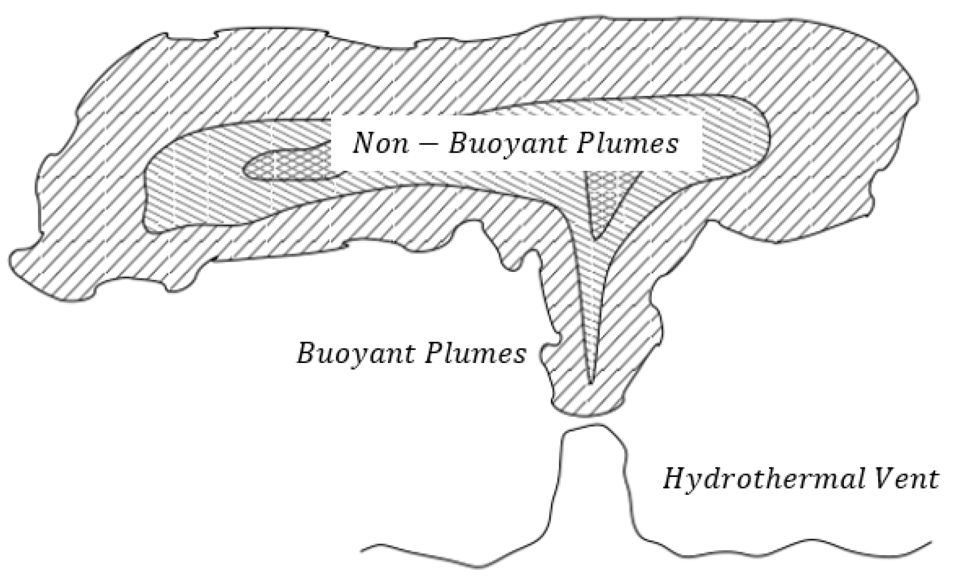
In this work, we present two new CPT algorithms for using on AUVs to trace emitted chemical plumes and find hydrothermal vent locations. First of all, we model the plume tracing of hydrothermal vent as a 2-dimensional (2-D) search problem. This is because the emitted hydrothermal plumes is mainly diffused on a fixed depth in an underwater environment. As shown in Figure 1, the structure of the emitted hydrothermal plumes comprises two components, namely buoyant and non-buoyant plumes. The non-buoyant plumes could range from tens of hundreds of kilometers at a fixed altitude above the seafloor [17]. Therefore, we simplify the hydrothermal vent localization problem on a 2-D plane search problem, where the AUV aims to find the hydrothermal vent on a horizontal plane of non-buoyant plumes. This simplification can also be found in other CPT applications, such as [13,50,51].
Figure 2 shows the flow diagram of the proposed CPT algorithm. During the plume tracing process, onboard sensors on the AUV measure AUV’s positions , flow speed and direction , chemical concentration , and AUV’s current heading . Sensor measurements will be fed into two modules, including a DNN (trained by DDPG or DDQN) and traditional CPT methods. Specifically, two traditional CPT methods are implemented, including the moth-inspired method [17] and the Bayesian-inference method [18]. Two traditional methods will generate two heading commands, i.e., and , based on the current sensor readings. On the other hand, the DNN also takes sensor measurements as inputs and calculates a fusion coefficient a. Here, a is a binary number if the DNN is trained by DDQN and a scalar if the DNN is trained by DDPG. Finally, the overall heading command is calculated by the superposition of and , where the weights are a and , respectively.
3.2. Moth-Inspired CPT Algorithm
The moth-inspired CPT algorithm is characterised in simplicity and high search efficiency in laminar flow environments. This section reviews the classic moth-inspired CPT method [17] that we implemented in this work.
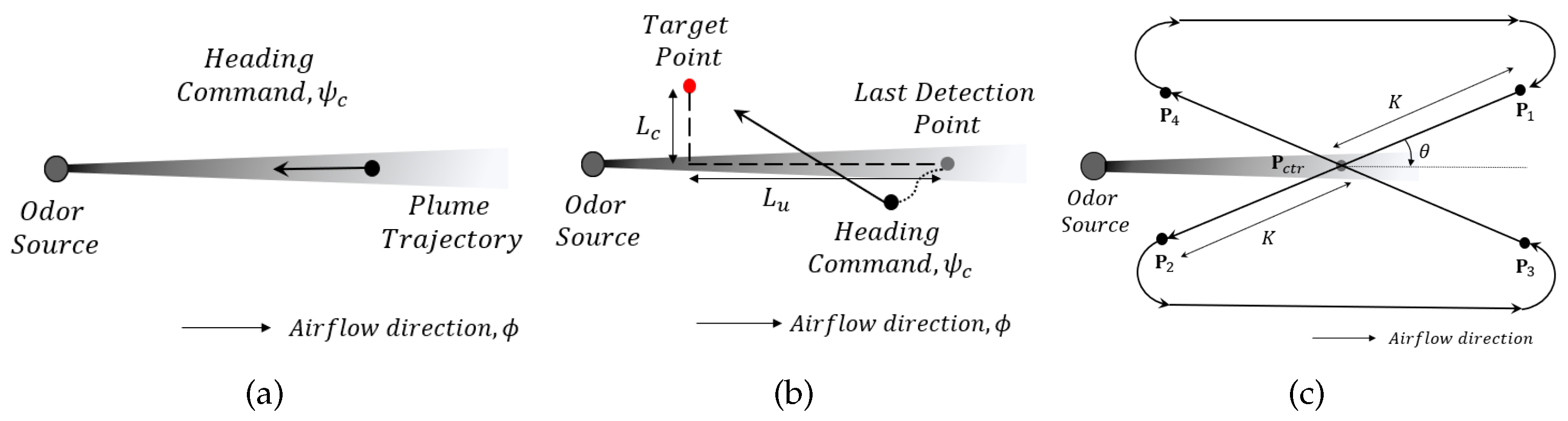
The moth-inspired method can be summarized as the alternation of ‘surge’ and ‘casting’ behaviors. Figure 3 presents the implementation of moth-inspired CPT algorithm proposed in [17], which further splits the ‘surge’ behavior as ‘track-in’ and ‘track-out’ behaviors. Specifically, in the ‘track-in’ behavior (as shown in Figure 3a), the AUV detects chemical plumes and moves upwind to approach the chemical source. In the ‘track-out’ behavior (as shown in Figure 3b), the AUV moves outside of plume areas and tries to re-detect plumes in the nearby of last detection location by moving across the plume trajectory. If the AUV fails to re-detect plumes in this behavior, then the ‘casting’ behavior (in [17], this behavior was called ‘reacquire’ behavior) is activated, which commands the robot to perform crosswind excursions to detect chemical plumes over a large area. As shown in Figure 3c, the ‘casting’ behavior was modeled as a ‘bow-tie’ trajectory, where the AUV was commanded to move to four points, i.e., to around the last plume detection location, i.e., . The AUV will turn back to the ‘track-in’ behavior if it detects chemical plumes. The AUV repeats these search behaviors until it finds the chemical source.
The ‘track-in’ behavior in the moth-inspired method CPT method can quickly guide the AUV to approach the chemical source in a laminar flow environment. In turbulent flow environment, the AUV cannot continuously detect chemical plumes since plume trajectory is not continuous but a patchy and intermittent trajectory. Therefore, the moth-inspired method is not efficient in turbulent flow environments since the AUV can only relay on ‘casting’ behavior to re-detect plumes. To mitigate this problem, we also include an engineering-based method that can estimate possible chemical source locations when the AUV loses plume contact in our CPT algorithm’s design.
3.3. Bayesian-Inference CPT Algorithm
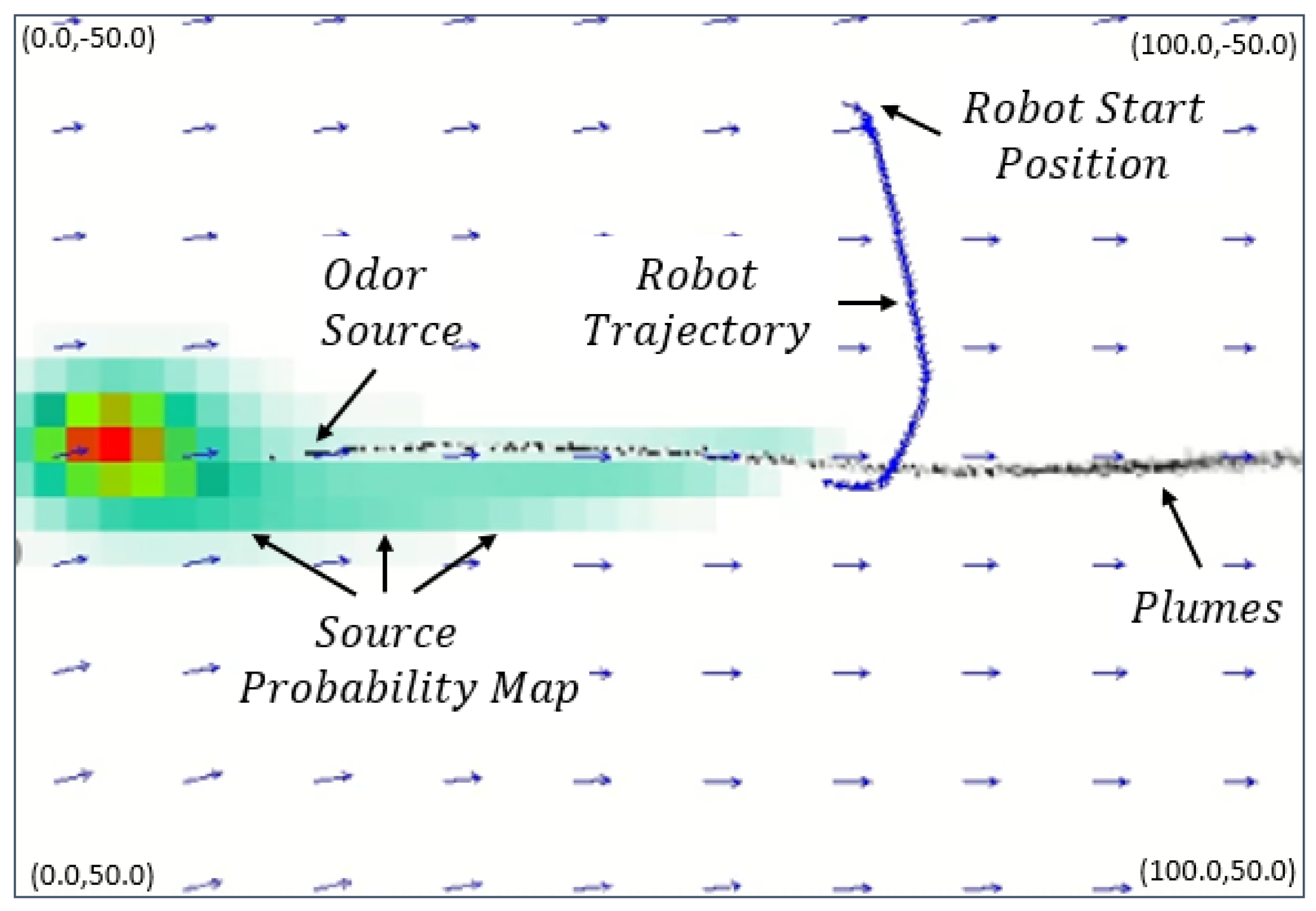
The Bayesian-inference method [18] models the plume movements as a Gaussian random process and estimates possible chemical source locations with sensed flow information. In this method, the search area was divided into multiple cells, where each cell has a probability of containing the chemical source. With the AUV maneuver, the probability of containing the chemical source in each cell was updating based on the plume detection and non-detection events. Figure 4 presents the source probability map in a search trial. In this diagram, the red cell indicates the estimate source location, i.e., the cell with the highest probability of containing the chemical source. In our previous simulation and real-world experiments [52], we found that the Bayesian-inference CPT algorithm is more effective than the moth-inspired CPT algorithm in a turbulent flow environment. This is because the source estimation in the Bayesian-inference method is calculated based on the previous plume information. When the AUV loses the plume contact, instead of randomly moving in a wide region and hoping to detect plumes by accident, the source estimation is more instructive to efficiently find the chemical source location since it pinpoints the possible source location.
3.4. RL Basics
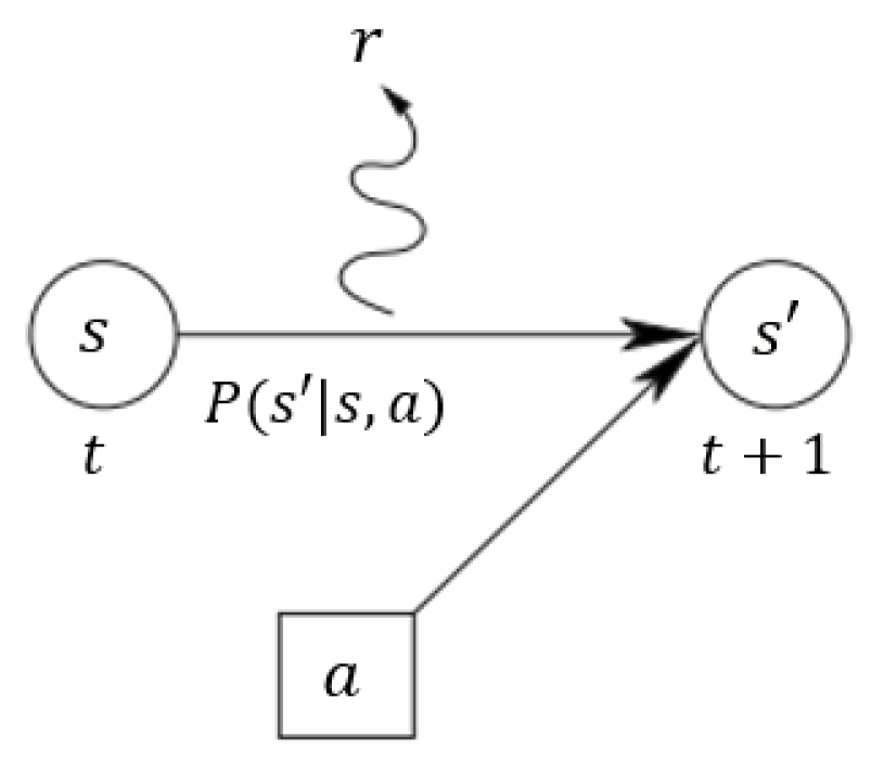
The standard RL setting contains an agent and an environment, and the interaction between the agent and the environment is modeled as a Markov decision process (MDP), where is a set of states, is a set of actions, P is a transition probability, R is a reward function, and is a discounting factor for future rewards. Figure 5 shows a MDP model within one time step. The agent is in a state (, ) at time t, and after it takes an action (, ) to arrive in the next state (, ) with the state transition probability , the agent will obtain a reward (, ).
An episode describes how the agent interacts with the environment. The policy () describes which action the agent will take in the state . The policy can be considered as a mapping function from state to action . The goal of the agent is to obtain a policy that maximizes the cumulative reward, which can be represented as: .
The value function is a prediction of the future reward. There are two kinds of value functions: state-value function and action-value function. The state-value function (i.e., ) evaluates the goodness of the agent being in a state s, and the action-value function (i.e., ) evaluates the goodness of the agent performs an action a in a state s. Mathematically, is the expectation of the return (total future rewards) starting from the current state , and then following the policy : ; is the expectation of the return starting from state s, taking the action a, and then following the policy : .
4. Deep RL-Based CPT Algorithms
Both DDQN and DDPG belong to model-free RL algorithms (i.e., deep RL), where the main difference is that DDQN has a discrete action space, and DDPG has a continuous action space. This section presents how to implement these two deep RL algorithms to train a DNN that can fuse heading commands of traditional CPT methods.
4.1. DDQN-Based CPT Method
The DDQN algorithm originates from the Q-learning and deep Q-network (DQN). In the Q-learning algorithm, every state-action pair has an action-value function, i.e., . At every time step, the agent selects the action with the highest action-value function, i.e., . However, if the state space is large, iterating all state-action pairs becomes time-consuming and even impossible. To solve this problem, DQN [11] trained a DNN to calculate action-value functions for arbitrary state-action pairs, i.e., . Thus, instead of calculating action-value functions for all state-action pairs in every time step, the agent relies on a DNN to estimate the action-value function for a given state-action pair. Two important ingredients are used in the DQN method to stabilize the training process, including the use of the target network and a experience replay.
Double Deep Q-Network [19] is a variant of DQN. In DQN, the target Q value is calculated based on the maximal action-value function, i.e., . This calculation introduces an overestimation in action-value functions and results in overoptimistic value estimates. Due to this reason, DDQN is proposed to reduce overestimations by decomposing the max operation in the target into two steps, i.e., action selection and action evaluation. In DDQN, the target is calculated as . This equation contains two steps: (1) action selection: the agent chooses an action a that results in the maximal ; (2) action evaluation: the target network estimate the action-value function based on the proposed action a.
Algorithm 1 presents the DDQN training algorithm. To adapt the DDQN algorithm into the CPT problem, we select the state s as sensor measurements. Onboard sensor measurements include flow speed and direction (v, ), AUV’s speed and heading (u, ), and chemical plume concentration . In choosing state variables, we convert angle-related variables, including flow direction () and AUV heading angles () to vector forms, such as , , , and . This is because angles do not make a good DNN input: one angle could refer to two different values, such as and , and angles should not matter if the corresponding speed is zero. Besides, we select the plume non-detection period as one of the states since it can reflect whether the AUV is maintaining inside plumes (, where is the last plume detection time). In summary, the state s can be presented as
There are two possible actions in the action space, i.e., . When the action is activated, the AUV will select the moth-inspired method as the current CPT algorithm, and if is activated, the AUV will choose the Bayesian-inference method as the current CPT strategy. We define reward functions as follows:
| Algorithm 1 DDQN Training Method |
|
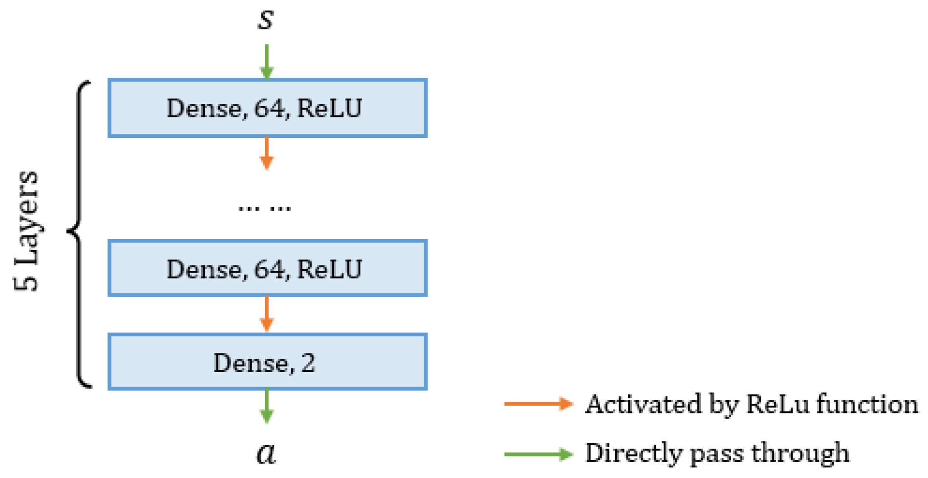
We consider that the AUV finds the source if the distance between the AUV and the source is less than a threshold (3 m in the simulation program). Hyper-parameters in Algorithm 1 are defined as follows: , , , , and , where N is the size of the replay buffer, L is the size of the mini-batch, is the probability of choosing random actions, is the discount factor, and C is the frequency of updating the target Q network. The architecture of the implemented DNN is presented in Figure 6, which is a 5-layer feedforward neural network with the ReLU activation function [54].
4.2. DDPG-Based CPT Method
The original DDPG algorithm employs the actor-critic architecture. There are two DNNs in the original DDPG algorithm, including an actor DNN and a critic DNN. The actor DNN calculates an action a (a continuous variable) based on the current state s, and the critic DNN calculates the action-value function to evaluate the actor’s action selection. The goal of the actor network is to choose an action that maximizes the action-value function, and the critic network aims to improve the accuracy of estimate the expected reward return. Similar to the DDQN algorithm, the DDPG algorithm also utilizes the target networks and experience replay to stabilize the training process. Specifically, both actor and critic networks have target networks. Target networks are initialized as clones of actor and critic networks and get updated gradually in a rate of during the training process. Transitions, i.e., , in an episode will be stored in a replay memory for repeatedly using during the training process.
Algorithm 2 presents the DDPG training algorithm. Specifically, the state s is identical to the one in the DDQN-based CPT algorithm, i.e., . The action calculated by the actor network is a scalar, ranging from 0 to 1. This scalar is the fusion coefficient that will be used to combine heading commands generated by two traditional CPT methods. Besides, the DDPG employs the same reward function as defined in the DDQN algorithm (see Equation (2)), i.e., the AUV receives positive rewards if it detects or find hydrothermal vent locations and negative rewards if it runs out of search time limit or moves out of the search area. The random noise is modeled as a Gaussian white noise with zero mean and 10 variance. The purpose of adding random noise on the action allows the agent to explore more actions and states during the training.
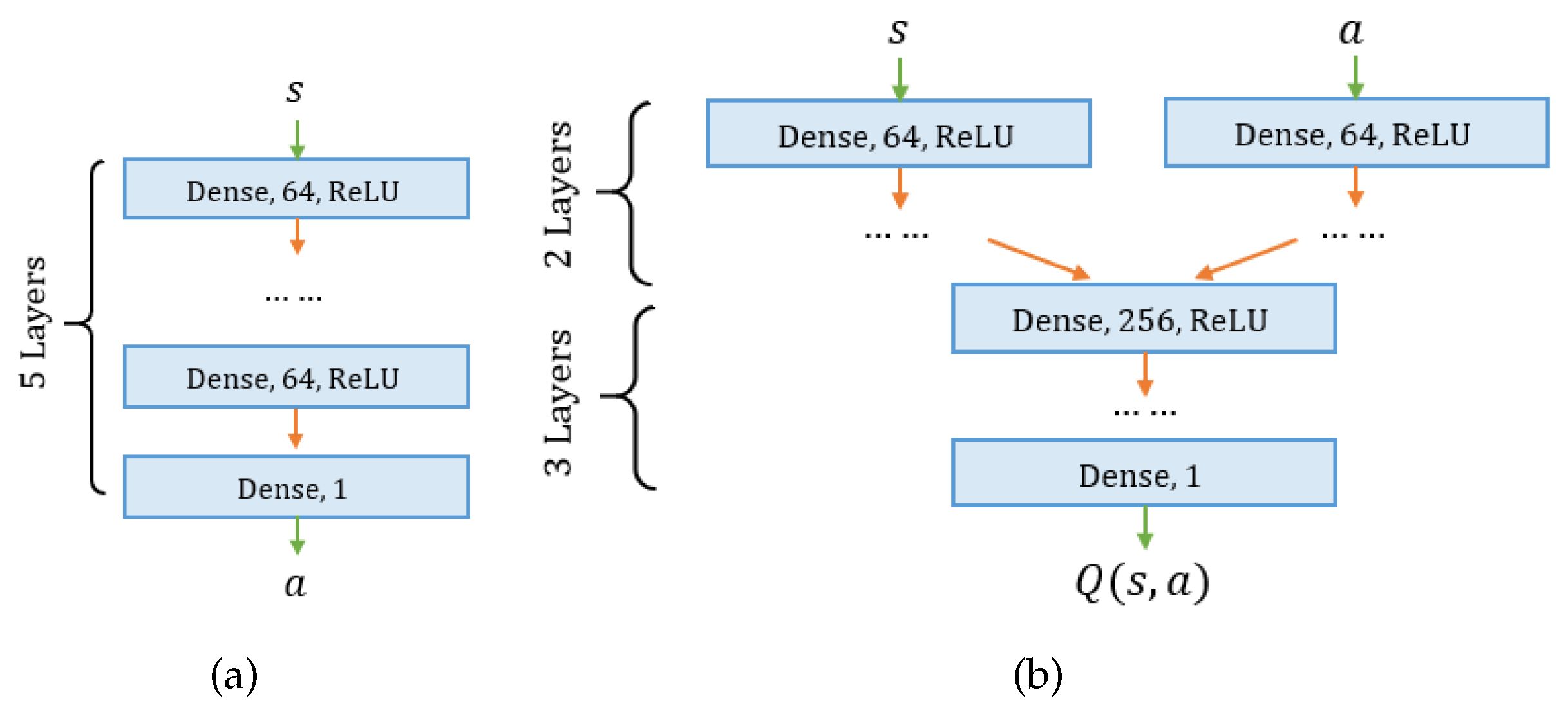
Similar to the previous DDQN algorithm, we consider the AUV finds the hydrothermal vent if the AUV’s position is within a small region of the hydrothermal vent (3 m in the simulation program). The output of the critic network is the action-value function associated with the current state s and action a. Hyper-parameters in Algorithm 2 are defined as follows: , , , and . Figure 7 presents the employed actor and critic networks in the DDPG algorithm. Both DNNs contains 5 dense layers, i.e., fully connected neural networks. Specifically, inputs of the actor network is state s, defined based on AUV’s sensor measurements, and the output is an action a, i.e., a fusion coefficient that ranging from 0 to 1. The critic network’s inputs include state s and the ation a. Each input is processed by two dense layers and then concatenated together to feed into three dense layers. The output of the critic network is the action-value function . The activation function in the actor and critic networks is ReLU.
| Algorithm 2 DDPG Training Method |
|
5. Simulation and Results
In this section, we evaluate the effectiveness of the proposed CPT algorithms and compare the search results with traditional moth-inspired [17] and Bayesian-based [18] methods (without the fusion) in a simulation program.
5.1. Simulation Setup
5.1.1. Simulated Environment
The simulation program used in this work was built based on [8]. This simulation program can present graphical animation to show how chemical plumes develop and how the agent searches the chemical source in the search environment. The simulation includes a time-varying flow field, a coherent chemical plume trajectory, and a full six degree of freedom autonomous vehicle dynamics. This simulation program is also utilized by [55,56,57,58,59] to study CPT algorithms.
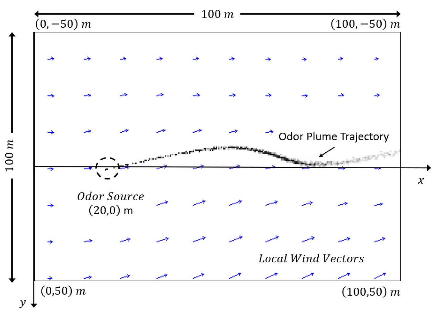
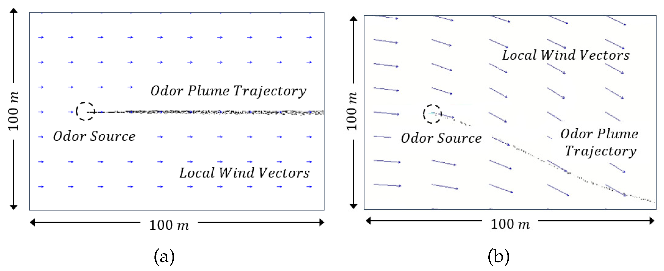
Figure 8 shows the search area in the simulation. The size of the search area is m. A coordinate () is constructed to represent positions. Under the coordinate, the hydrothermal vent is located at m and releases 10 filament packages (i.e., plumes) per second. Grey dots in the center represent released plumes and form a curvy plume trajectory. Arrows in the background represent flow vectors, where an arrow points to the flow direction and the length of an arrow indicates the strength of flow velocity. In this simulator, flow vectors are calculated from time-varying boundary conditions that are generated by a mean flow () and a Gaussian white noise (zero mean and variance). By changing values of and , different amplitudes of airflow fields can be obtained. Figure 9 shows examples of two different flow environments: a laminar airflow environment was created with m/s and in Figure 9a, and in Figure 9b, a turbulent airflow environment was generated with m/s and .
5.1.2. Vehicle Assumptions
In the simulation program, the vehicle dynamic is modeled based on a real-world AUV, i.e., the REMUS 100 AUV [60]. Comparing to the large scale of the search area, the size of the AUV is negligible. Therefore, the AUV is approximated as a single point in the simulation program. It is assumed that the AUV is equipped with a chemical sensor, a flow sensor, and a positioning sensor, which measure chemical plume concentrations at the AUV position, water flow speeds and directions in the inertial frame, and AUV positions in the inertial frame, respectively. To mimic the real-world applications, all sensors’ measurements are corrupted with Gaussian white noises. The noise parameters are listed in Table 1. The proposed CPT algorithms are implemented on an onboard computer to process sensor readings and calculate the heading commands, which is limited in a range of . The AUV’s velocity set as a constant to simplify the control problem, i.e., 1 m/s.
5.2. Training Results
The proposed DDQN- and DDPG-based CPT algorithms were trained in the aforementioned simulation program. Specifically, each algorithm was trained 4000 episodes. For each training episode, the AUV initial position was randomly sampled at the downflow area of the hydrothermal vent (i.e., m and m), and the flow condition in the search environment varied. The training time for a single algorithm was around 4 h on a workstation computer with an Intel Core i9 CPU and Nvidia RTX 3090 GPU.
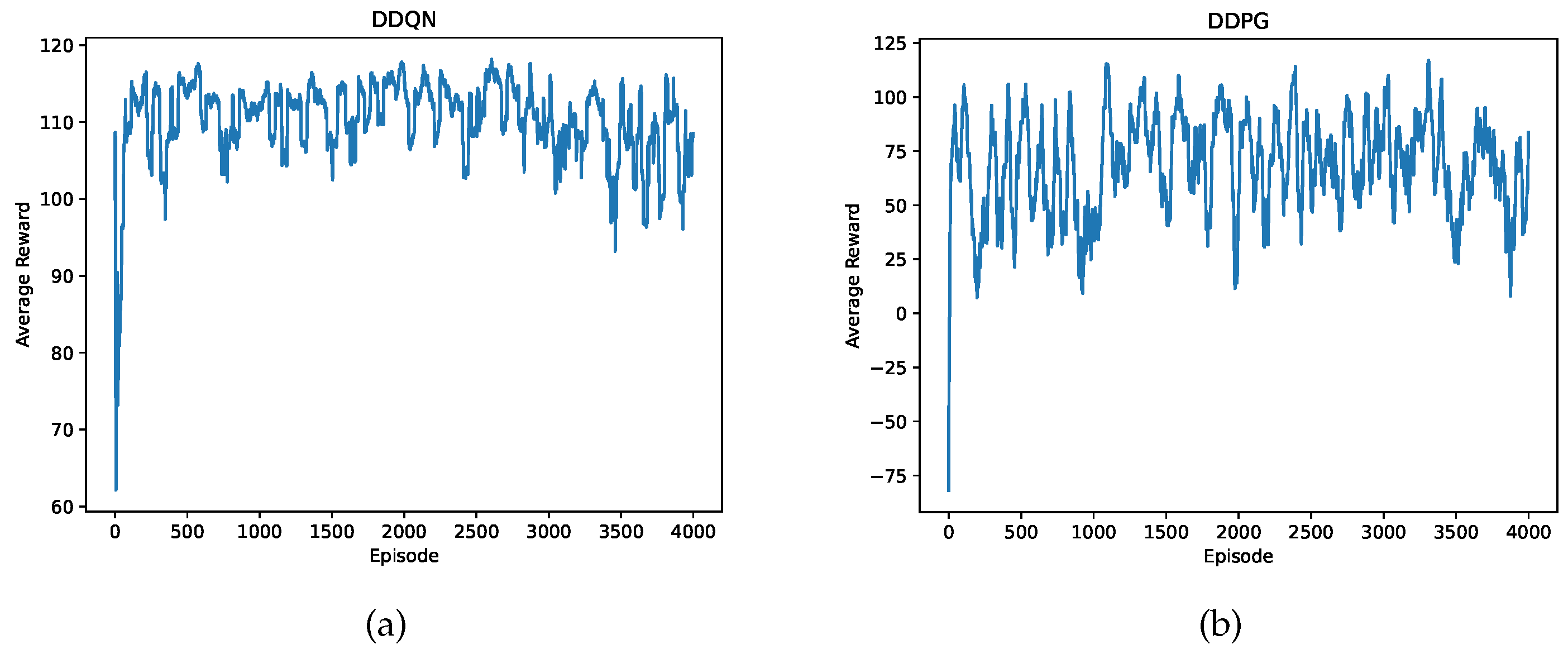
Figure 10 presents the averaged reward plots for the proposed DDQN- and DDPG-based CPT algorithms. We can see that both plots maintain at a high value after around 200 episodes, indicating the agent achieved a high success rate of finding hydrothermal vents. Besides, the averaged reward obtained by the agent trained by DDQN is higher than the DDPG counterpart. This is because the proposed DDQN-based CPT algorithm switches between moth-inspired and Bayesian-inference methods during the search, which is more instructive than the fusion of heading commands in the DDPG-based CPT algorithm. In the early training episodes, the fusion coefficient calculated by the DDPG’s actor network deteriorates the search efficiency since two traditional CPT methods may propose two opposite heading commands, and the fusion of two commands leads the AUV to an erroneous direction.
5.3. Simulation Results in Laminar Flow Environments
We first implement the proposed DDQN- and DDPG-based CPT algorithms in laminar flow environments where m/s and . We first present a sample search, performed by the proposed deep RL-based CPT algorithms. In the sample run, the AUV initial position is at m, and the source location is at m.
5.3.1. Sample Run of the Proposed DDQN-Based Algorithm
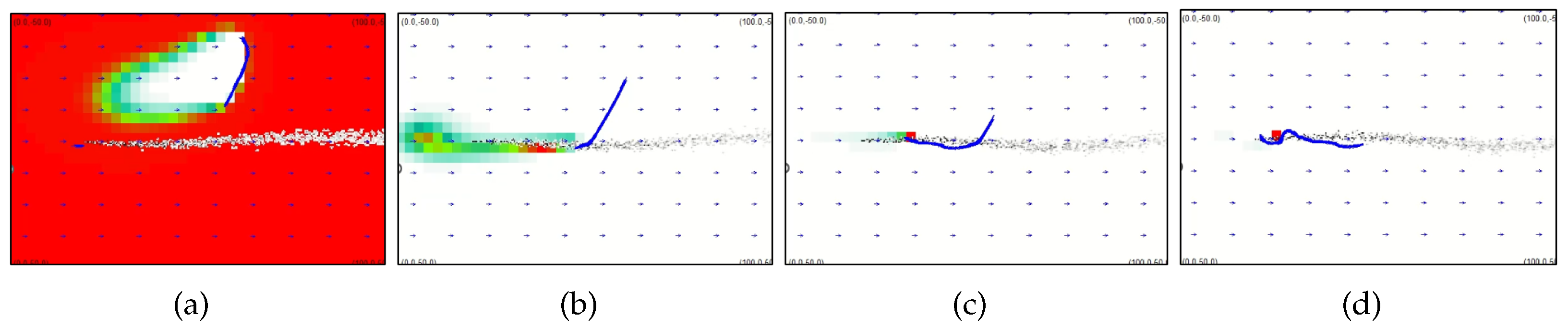
Figure 11 presents the snapshots of search trajectories generated by the DDQN-based CPT algorithm. As we can see in Figure 11a, the AUV employed the ‘zigzag’ search trajectory to search plumes for the first time. Details of the ‘zigzag’ behavior can be found in [52], which can be summarized as follows: the AUV will head in a crosswind direction and bounce inward the search area when it arrives at the boundaries of the search area. At s, the AUV contacted plumes for the first time and switched to the proposed DDQN-based CPT algorithm. At this time, the DNN selected the Bayesian-inference method as the search algorithm. Thus, the AUV moves to the red region in the search area as presented in Figure 11b, which is the region with the highest probability of containing the hydrothermal vent. From s to s, the AUV was directed by the Bayesian-inference method to move upflow since the DNN’s output is 1. After s, the DNN’s output becomes , commanding the AUV to follow the moth-inspired method to quickly approach the source location. As indicated in Figure 11d, the AUV correctly find the hydrothermal vent’s location at s.
5.3.2. Sample Run of the Proposed DDPG-Based Algorithm
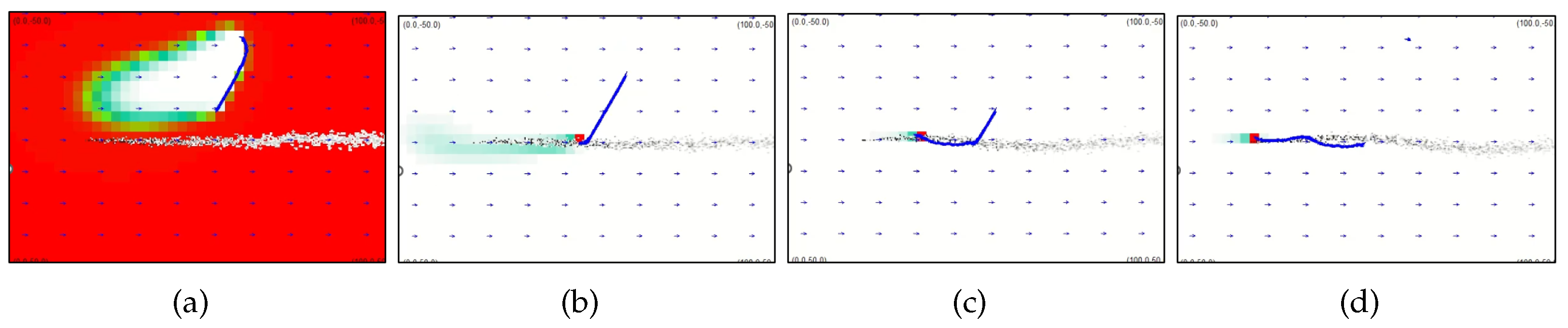
Figure 12 presents the snapshots of search trajectories generated by the DDPG-based CPT algorithm. Similar to the DDQN-based CPT algorithm, the AUV successfully finds the hydrothermal vent’s location at the end of the search. Comparing to the DDQN counterpart, the DDPG commands the AUV to use moth-inspired CPT algorithm in the most of search time (i.e., the fusion coefficient is larger than 0.5). Specifically, the AUV first employed the ‘zigzag’ search trajectory to find the existence of plumes in the environment. At s, the AUV detected plumes for the first time and switched to the DDPG-based CPT algorithm. As indicated in Figure 12c, the AUV stayed inside plumes and moved upflow to approach the source location. At s, the AUV correctly found the source location.
5.3.3. Repeated Tests in Laminar Flows
We also implemented the proposed deep RL-based CPT algorithms in repeated tests and compared the statistic results with traditional CPT algorithms. Four CPT algorithms, including DDQN, DDPG, moth-inspired, and Bayesian-inference methods were implemented in the simulation program, and each method was repeatedly performed 100 times. In repeated tests, the AUV initial position was selected from four possible candidates, including m, m, m. and m. The AUV performed 25 trials at each initial position with four CPT algorithms, i.e., the proposed DDQN, DDPG, the traditional moth-inspired, and Bayesian-inference methods. The search time limit for a trial is 400 s. If the AUV cannot find the hydrothermal vent within the time limit, this trial will be considered as an unsuccessful trial in locating the hydrothermal vent. Table 2 presents the results of repeated tests.
From Table 2, we can see that the proposed DDQN-based CPT algorithm outperforms traditional moth-inspired and Bayesian-inference methods, where the success rate of the DDQN is 100 % versus 99% for the traditional moth-inspired and 90% for the Bayesian-inference method. The averaged search time for the DDQN is also shorter than two traditional methods. The proposed DDPG-based CPT algorithm achieves a better search performance than the Bayesian-inference method, where the success rate is 98% versus 90% for the Bayesian-inference method and the averaged search time is 3 s shorther than the Bayesian-inference counterpart. As for two traditional methods, we can see that the moth-inspired method achieves a shorter averaged search time than the Bayesian-inference method thanks to the effective ‘track-in’ behavior that can quickly lead the AUV to move upflow and approach the hydrothermal vent. The proposed DDQN-based CPT algorithm outperforms the moth-inspired method, indicating the effectiveness of the proposed DDQN-based CPT algorithm and the idea that combining bio-inspired and engineering-based methods benefits in improving the search performance.
5.4. Simulation Results in Turbulent Flow Environments
In this section, the proposed deep RL-based CPT algorithms will be implemented in turbulent flow environments, where m/s and . Similar to the previous group of tests, we first present sample runs of the proposed CPT algorithms in turbulent flow environments. The AUV initial position is at m, and the source location is at m.
5.4.1. Sample Run of the Proposed DDQN-Based Algorithm
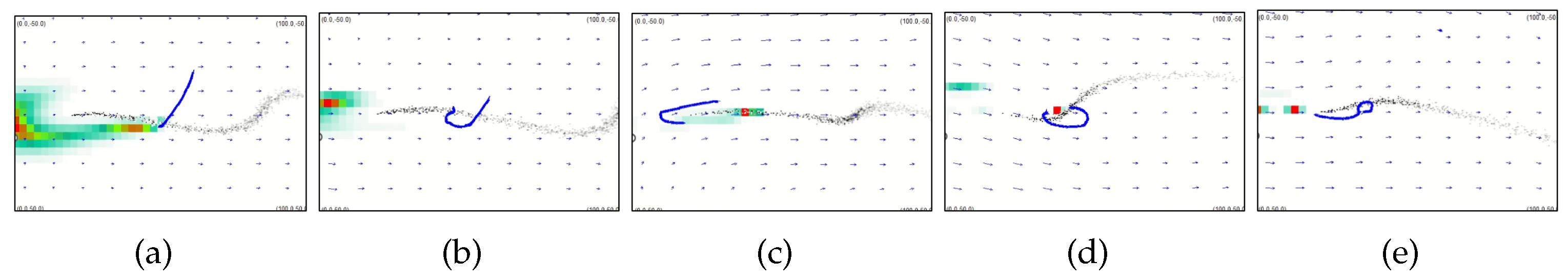
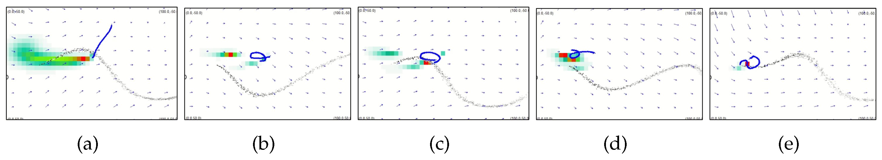
Figure 13 presents the snapshots of search trajectory generated by the DDQN-based CPT algorithm. Specifically, the AUV adapted the ‘zigzag’ search trajectory to find chemical plumes in the search environment and detected chemical plumes for the first time at s as indicated in Figure 13a. At s, the AUV adapted the Bayesian-inference method as commanded by the DDQN-based CPT algorithm and moved to the estimated source location (i.e., the red region in Figure 13b). At s, the AUV did not detect chemical plumes at the estimated source location and updated the source estimate as presented in Figure 13c. At s, i.e., Figure 13d, the AUV switched to the moth-inspired method and successfully detected the chemical plumes. At s, the AUV switched back into the Bayesian-inference method and correctly found the hydrothermal vent’s location, as presented in Figure 13e.
5.4.2. Sample Run of the Proposed DDPG-Based Algorithm
Figure 14 shows the snapshots of search trajectory produced by the DDPG-based CPT algorithm. From these diagrams, we can see that the plume trajectory (i.e., black particles) is very curvy due to the turbulent flows. Thus, it will be very inefficient if the AUV chooses the moth-inspired method since the AUV will spend a lot of time on the ‘casting’ behavior to re-detect plumes.
In this test, we observed that the DDPG’s output, i.e., the fusion coefficient, is 0 in most of the search time, indicating that the DDPG selected the Bayesian-inference method over the moth-inspired method, considering that the Bayesian-inference method is more effective than moth-inspired method in finding hydrothermal vents in turbulent flow environments. This observation indicates that the DDPG algorithm learns how to choose correct search strategy in different search environments. Specifically, the AUV detected the first plume at s after the ‘zigzag’ search strategy as presented in Figure 14a. From s to s, the AUV was directed by the Bayesian-inference method and detected chemical plumes several times in the nearby of the plume trajectory as indicated by Figure 14b,c. At s, the AUV was close to the source location thanks to the guidance of accurate source estimate as presented in Figure 14d. In Figure 14e, the AUV correctly found the source location at s.
5.4.3. Repeated Tests in Turbulent Flows
To verify the effectiveness and robustness of the proposed deep RL-based algorithms in turbulent flow environments, we implemented the proposed algorithms in repeated tests. Similar to the tests in laminar flow environments, the AUV started at four different initial positions, i.e., m, m, m, and m. Besides the proposed deep RL-based algorithms, the traditional moth-inspired and Bayesian-inference methods were also implemented in this group of tests. Table 3 lists statistic results of the proposed deep RL-based CPT algorithms and traditional methods in repeated tests. As we can see, the DDQN-based CPT algorithm achieves the best performance in this group of tests, where the success rate is 94% in 100 tests and the averaged search time and standard deviation are 96.3 s and 68.5, respectively. The DDPG-based algorithm also outperforms traditional methods in turbulent flow environments, where the success rate is , averaged search time is s, and standard deviation is 115.3. Statistic results in repeated tests show the effectiveness of the proposed deep RL-based algorithms in turbulent flow environments.
5.5. Discussion
We compared our proposed methods with an end-to-end RL algorithm proposed in [13]. According to the reported search performance (i.e., Table 1 in [13]), our proposed method achieved a comparable search performance in terms of the success rate. The highest success rate in [13] is 98.81% (the number of repeated tests is unspecified in [13]), and our double deep Q-network method achieved a 100% success rate in 100 repeated tests (see Table 2). It is also worth mentioning that our neural network structure is much simpler than the one proposed in [13], which needs less calculation time to process the input data.
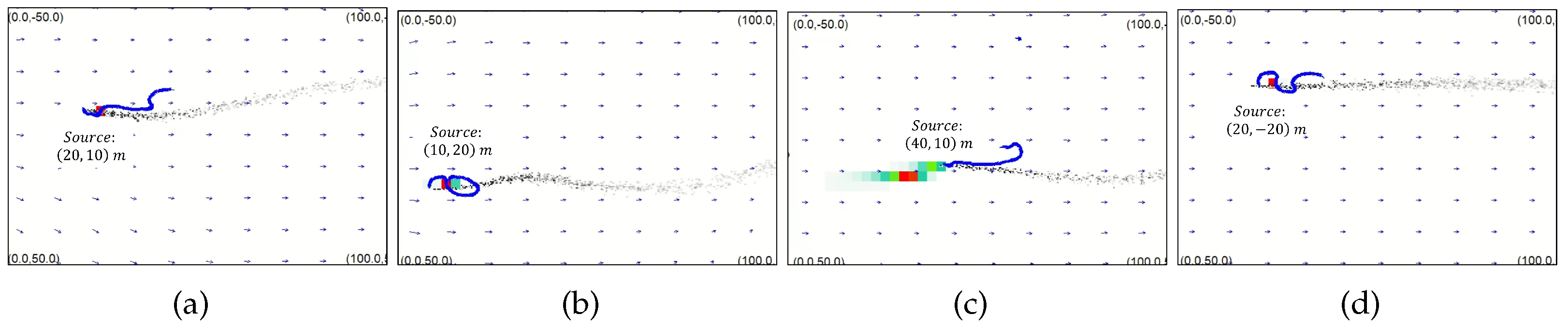
We also evaluated the search performance of proposed methods in different source locations. Figure 15 shows snapshots of four trials with different source locations, including m, m, m, and m. We can see that the AUV successfully reached the hydrothermal vent location at the end of each trial. Simulation results reflect the effectiveness of the proposed CPT algorithms. In the future, we plan to implement the proposed CPT algorithms in real-world environments and study on more complicated search scenarios, such as searching with multiple AUVs and multiple odor sources.
6. Conclusions
In this paper, we present two deep RL-based CPT algorithms. Two deep RL algorithms, including DDQN and DDPG, are employed to design CPT algorithms for using on AUVs to locate underwater hydrothermal vents. Considering the low sample efficiency of deep RL algorithms, we employed deep RL algorithms to train DNNs that calculates a fusion coefficient to combine two traditional CPT algorithms, i.e., moth-inspired and Bayesian-inference methods. Specifically, the DDQN algorithm selects one search strategy from two traditional methods during the search process, while the DDPG algorithm calculates a fusion variable that combines two traditional methods in a superposition format. Based on simulation tests, we found that both deep RL-based algorithms are effective in finding hydrothermal vents in both laminar and turbulent flow environments. Besides, comparing to traditional CPT algorithms, i.e., without the fusion, the search performance is improved in terms of the averaged search time and success rate. In laminar flow environments, both DDQN- and DDPG-based CPT algorithms achieve a high success rate (>90%) in 100 repeated trials. In turbulent flow environments, our proposed DDQN achieved the best performance, which improves the search success rate by 67% compared to the moth-inspired method and 34% compared to the Bayesian-inference method. Simulation results indicate the effectiveness of the proposed CPT methods in both laminar and turbulent flow environments.
Author Contributions
Conceptualization, L.W. and S.P.; methodology, software, validation, formal analysis, investigation, resources, writing—original draft preparation, L.W.; writing—review and editing, S.P.; supervision, L.W. All authors have read and agreed to the published version of the manuscript.
Funding
This research received no external funding.
Conflicts of Interest
The authors declare no conflict of interest.
References
- Luther, G.W.; Rozan, T.F.; Taillefert, M.; Nuzzio, D.B.; Di Meo, C.; Shank, T.M.; Lutz, R.A.; Cary, S.C. Chemical speciation drives hydrothermal vent ecology. Nature 2001, 410, 813–816. [Google Scholar] [CrossRef] [PubMed]
- Martin, W.; Baross, J.; Kelley, D.; Russell, M.J. Hydrothermal vents and the origin of life. Nat. Rev. Microbiol. 2008, 6, 805–814. [Google Scholar] [CrossRef] [PubMed]
- German, C.R.; Lin, J. The thermal structure of the oceanic crust, ridge-spreading and hydrothermal circulation: How well do we understand their inter-connections. Mid-Ocean Ridges Hydrothermal Interact. Lithosphere Ocean. Geophys. Monogr. Ser 2004, 148, 1–18. [Google Scholar]
- Ferri, G.; Jakuba, M.V.; Yoerger, D.R. A novel trigger-based method for hydrothermal vents prospecting using an autonomous underwater robot. Auton. Robot. 2010, 29, 67–83. [Google Scholar] [CrossRef]
- Kelley, D.S.; Karson, J.A.; Früh-Green, G.L.; Yoerger, D.R.; Shank, T.M.; Butterfield, D.A.; Hayes, J.M.; Schrenk, M.O.; Olson, E.J.; Proskurowski, G.; et al. A serpentinite-hosted ecosystem: The Lost City hydrothermal field. Science 2005, 307, 1428–1434. [Google Scholar] [CrossRef]
- Chen, X.X.; Huang, J. Odor source localization algorithms on mobile robots: A review and future outlook. Robot. Auton. Syst. 2019, 112, 123–136. [Google Scholar] [CrossRef]
- Zhu, Y.; Mottaghi, R.; Kolve, E.; Lim, J.J.; Gupta, A.; Fei-Fei, L.; Farhadi, A. Target-driven visual navigation in indoor scenes using deep reinforcement learning. In Proceedings of the 2017 IEEE international conference on robotics and automation (ICRA), Singapore, 29 May–3 June 2017; pp. 3357–3364. [Google Scholar]
- Farrell, J.A.; Murlis, J.; Long, X.; Li, W.; Cardé, R.T. Filament-based atmospheric dispersion model to achieve short time-scale structure of odor plumes. Environ. Fluid Mech. 2002, 2, 143–169. [Google Scholar] [CrossRef]
- Sutton, R.S.; Barto, A.G. Reinforcement Learning: An Introduction; MIT Press: Cambridge, MA, USA, 2018. [Google Scholar]
- Nguyen, H.; La, H. Review of deep reinforcement learning for robot manipulation. In Proceedings of the 2019 Third IEEE International Conference on Robotic Computing (IRC), Naples, Italy, 25–27 February 2019; pp. 590–595. [Google Scholar]
- Mnih, V.; Kavukcuoglu, K.; Silver, D.; Graves, A.; Antonoglou, I.; Wierstra, D.; Riedmiller, M. Playing atari with deep reinforcement learning. arXiv 2013, arXiv:1312.5602. [Google Scholar]
- Silver, D.; Huang, A.; Maddison, C.J.; Guez, A.; Sifre, L.; Van Den Driessche, G.; Schrittwieser, J.; Antonoglou, I.; Panneershelvam, V.; Lanctot, M.; et al. Mastering the game of Go with deep neural networks and tree search. Nature 2016, 529, 484–489. [Google Scholar] [CrossRef]
- Hu, H.; Song, S.; Chen, C.P. Plume Tracing via Model-Free Reinforcement Learning Method. IEEE Trans. Neural Netw. Learn. Syst. 2019, 8, 2515–2527. [Google Scholar] [CrossRef]
- Singh, S.H.; van Breugel, F.; Rao, R.P.; Brunton, B.W. Emergent behavior and neural dynamics in artificial agents tracking turbulent plumes. arXiv 2021, arXiv:2109.12434. [Google Scholar]
- Silver, D.; Lever, G.; Heess, N.; Degris, T.; Wierstra, D.; Riedmiller, M. Deterministic policy gradient algorithms. In Proceedings of the International Conference on Machine Learning, PMLR, Bejing, China, 22–24 June 2014; pp. 387–395. [Google Scholar]
- Silver, D.; Schrittwieser, J.; Simonyan, K.; Antonoglou, I.; Huang, A.; Guez, A.; Hubert, T.; Baker, L.; Lai, M.; Bolton, A.; et al. Mastering the game of go without human knowledge. Nature 2017, 550, 354–359. [Google Scholar] [CrossRef] [PubMed]
- Farrell, J.A.; Pang, S.; Li, W. Chemical plume tracing via an autonomous underwater vehicle. IEEE J. Ocean. Eng. 2005, 30, 428–442. [Google Scholar] [CrossRef]
- Pang, S.; Farrell, J.A. Chemical plume source localization. IEEE Trans. Syst. Man Cybern. Part (Cybernetics) 2006, 36, 1068–1080. [Google Scholar] [CrossRef]
- Van Hasselt, H.; Guez, A.; Silver, D. Deep reinforcement learning with double q-learning. In Proceedings of the AAAI Conference on Artificial Intelligence, Phoenix, AZ, USA, 12–17 February 2016; Volume 30. number 1. [Google Scholar]
- Lillicrap, T.P.; Hunt, J.J.; Pritzel, A.; Heess, N.; Erez, T.; Tassa, Y.; Silver, D.; Wierstra, D. Continuous control with deep reinforcement learning. arXiv 2015, arXiv:1509.02971. [Google Scholar]
- Ishida, H.; Suetsugu, K.i.; Nakamoto, T.; Moriizumi, T. Study of autonomous mobile sensing system for localization of odor source using gas sensors and anemometric sensors. Sens. Actuators Phys. 1994, 45, 153–157. [Google Scholar] [CrossRef]
- Grasso, F.W.; Consi, T.R.; Mountain, D.C.; Atema, J. Biomimetic robot lobster performs chemo-orientation in turbulence using a pair of spatially separated sensors: Progress and challenges. Robot. Auton. Syst. 2000, 30, 115–131. [Google Scholar] [CrossRef]
- Russell, R.A.; Bab-Hadiashar, A.; Shepherd, R.L.; Wallace, G.G. A comparison of reactive robot chemotaxis algorithms. Robot. Auton. Syst. 2003, 45, 83–97. [Google Scholar] [CrossRef]
- Lilienthal, A.; Duckett, T. Experimental analysis of gas-sensitive Braitenberg vehicles. Adv. Robot. 2004, 18, 817–834. [Google Scholar] [CrossRef]
- Ishida, H.; Nakayama, G.; Nakamoto, T.; Moriizumi, T. Controlling a gas/odor plume-tracking robot based on transient responses of gas sensors. IEEE Sens. J. 2005, 5, 537–545. [Google Scholar] [CrossRef]
- Grasso, F.W.; Basil, J.A.; Atema, J. Toward the convergence: Robot and lobster perspectives of tracking odors to their source in the turbulent marine environment. In Proceedings of the 1998 IEEE International Symposium on Intelligent Control (ISIC) Held Jointly with IEEE International Symposium on Computational Intelligence in Robotics and Automation (CIRA) Intell, Gaithersburg, MD, USA, 17 September 1998; pp. 259–264. [Google Scholar]
- Michaelis, B.T.; Leathers, K.W.; Bobkov, Y.V.; Ache, B.W.; Principe, J.C.; Baharloo, R.; Park, I.M.; Reidenbach, M.A. Odor tracking in aquatic organisms: The importance of temporal and spatial intermittency of the turbulent plume. Sci. Rep. 2020, 10, 1–11. [Google Scholar] [CrossRef] [PubMed]
- Leathers, K.W.; Michaelis, B.T.; Reidenbach, M.A. Interpreting the spatial-temporal structure of turbulent chemical plumes utilized in odor tracking by lobsters. Fluids 2020, 5, 82. [Google Scholar] [CrossRef]
- Cardé, R.T.; Willis, M.A. Navigational strategies used by insects to find distant, wind-borne sources of odor. J. Chem. Ecol. 2008, 34, 854–866. [Google Scholar] [CrossRef] [PubMed]
- Lochmatter, T.; Raemy, X.; Matthey, L.; Indra, S.; Martinoli, A. A comparison of casting and spiraling algorithms for odor source localization in laminar flow. In Proceedings of the 2008 IEEE International Conference on Robotics and Automation, Pasadena, CA, USA, 19–23 May 2008; pp. 1138–1143. [Google Scholar] [CrossRef] [Green Version]
- Li, W.; Farrell, J.A.; Pang, S.; Arrieta, R.M. Moth-inspired chemical plume tracing on an autonomous underwater vehicle. IEEE Trans. Robot. 2006, 22, 292–307. [Google Scholar] [CrossRef]
- Pang, S. Plume source localization for AUV based autonomous hydrothermal vent discovery. In Proceedings of the OCEANS 2010 MTS/IEEE SEATTLE, Seattle, WA, USA, 20–23 September 2010; pp. 1–8. [Google Scholar]
- Shigaki, S.; Sakurai, T.; Ando, N.; Kurabayashi, D.; Kanzaki, R. Time-varying moth-inspired algorithm for chemical plume tracing in turbulent environment. IEEE Robot. Autom. Lett. 2017, 3, 76–83. [Google Scholar] [CrossRef]
- Shigaki, S.; Shiota, Y.; Kurabayashi, D.; Kanzaki, R. Modeling of the Adaptive Chemical Plume Tracing Algorithm of an Insect Using Fuzzy Inference. IEEE Trans. Fuzzy Syst. 2019, 28, 72–84. [Google Scholar] [CrossRef]
- Farrell, J.A.; Pang, S.; Li, W. Plume mapping via hidden Markov methods. IEEE Trans. Syst. Man, Cybern. Part B (Cybernetics) 2003, 33, 850–863. [Google Scholar] [CrossRef]
- Li, J.G.; Meng, Q.H.; Wang, Y.; Zeng, M. Odor source localization using a mobile robot in outdoor airflow environments with a particle filter algorithm. Auton. Robot. 2011, 30, 281–292. [Google Scholar] [CrossRef]
- Jakuba, M.; Yoerger, D.R. Autonomous search for hydrothermal vent fields with occupancy grid maps. In Proceedings of the ACRA, Canberra, Australia, 3–5 December 2008; Volume 8, p. 2008. [Google Scholar]
- Saigol, Z.A.; Dearden, R.W.; Wyatt, J.L.; Murton, B.J. Information-lookahead planning for AUV mapping. In Proceedings of the Twenty-First International Joint Conference on Artificial Intelligence, Pasadena, CA, USA, 11–17 July 2009. [Google Scholar]
- Jiu, H.f.; Pang, S.; Li, J.l.; Han, B. Odor plume source localization with a Pioneer 3 Mobile Robot in an indoor airflow environment. In Proceedings of the IEEE SoutheastCon 2014, Lexington, KY, USA, 13–16 March 2014; pp. 1–6. [Google Scholar]
- Wang, L.; Pang, S. Chemical Plume Tracing using an AUV based on POMDP Source Mapping and A-star Path Planning. In Proceedings of the OCEANS 2019 MTS/IEEE SEATTLE, Seattle, WA, USA, 27–31 October 2019; pp. 1–7. [Google Scholar]
- Vergassola, M.; Villermaux, E.; Shraiman, B.I. ‘Infotaxis’ as a strategy for searching without gradients. Nature 2007, 445, 406. [Google Scholar] [CrossRef]
- Kennedy, J.; Eberhart, R. Particle swarm optimization. In Proceedings of the ICNN’95-International Conference on Neural Networks, Perth, WA, USA, 27 November–1 December 1995; Volume 4, pp. 1942–1948. [Google Scholar]
- Marques, L.; Nunes, U.; de Almeida, A.T. Particle swarm-based olfactory guided search. Auton. Robot. 2006, 20, 277–287. [Google Scholar] [CrossRef]
- Fu, Z.; Chen, Y.; Ding, Y.; He, D. Pollution source localization based on multi-UAV cooperative communication. IEEE Access 2019, 7, 29304–29312. [Google Scholar] [CrossRef]
- Meng, Q.H.; Yang, W.X.; Wang, Y.; Zeng, M. Collective odor source estimation and search in time-variant airflow environments using mobile robots. Sensors 2011, 11, 10415–10443. [Google Scholar] [CrossRef] [PubMed]
- Lu, Q.; Luo, P. A learning particle swarm optimization algorithm for odor source localization. Int. J. Autom. Comput. 2011, 8, 371–380. [Google Scholar] [CrossRef]
- Wang, L.; Pang, S.; Li, J. Olfactory-Based Navigation via Model-Based Reinforcement Learning and Fuzzy Inference Methods. IEEE Trans. Fuzzy Syst. 2020, 29, 3014–3027. [Google Scholar] [CrossRef]
- Wang, L.; Pang, S.; Li, J. Learn to Trace Odors: Autonomous Odor Source Localization via Deep Learning Methods. In Proceedings of the 2021 20th IEEE International Conference on Machine Learning and Applications (ICMLA), Pasadena, CA, USA, 13–16 December 2021; pp. 1429–1436. [Google Scholar]
- Chen, X.; Fu, C.; Huang, J. A Deep Q-Network for robotic odor/gas source localization: Modeling, measurement and comparative study. Measurement 2021, 183, 109725. [Google Scholar] [CrossRef]
- Ferri, G.; Jakuba, M.V.; Mondini, A.; Mattoli, V.; Mazzolai, B.; Yoerger, D.R.; Dario, P. Mapping multiple gas/odor sources in an uncontrolled indoor environment using a Bayesian occupancy grid mapping based method. Robot. Auton. Syst. 2011, 59, 988–1000. [Google Scholar] [CrossRef]
- Jiu, H.; Chen, Y.; Deng, W.; Pang, S. Underwater chemical plume tracing based on partially observable Markov decision process. Int. J. Adv. Robot. Syst. 2019, 16, 1729881419831874. [Google Scholar] [CrossRef]
- Wang, L.; Pang, S. Robotic odor source localization via adaptive bio-inspired navigation using fuzzy inference methods. Robot. Auton. Syst. 2022, 147, 103914. [Google Scholar] [CrossRef]
- Sigaud, O.; Buffet, O. Markov Decision Processes in Artificial Intelligence; John Wiley & Sons: Hoboken, NJ, USA, 2013. [Google Scholar]
- Agarap, A.F. Deep learning using rectified linear units (relu). arXiv 2018, arXiv:1803.08375. [Google Scholar]
- Jatmiko, W.; Sekiyama, K.; Fukuda, T. A pso-based mobile robot for odor source localization in dynamic advection-diffusion with obstacles environment: Theory, simulation and measurement. IEEE Comput. Intell. Mag. 2007, 2, 37–51. [Google Scholar] [CrossRef]
- Lu, Q.; Han, Q.L.; Xie, X.; Liu, S. A finite-time motion control strategy for odor source localization. IEEE Trans. Ind. Electron. 2014, 61, 5419–5430. [Google Scholar] [CrossRef]
- Tian, Y.; Zhang, A. Simulation environment and guidance system for AUV tracing chemical plume in 3-dimensions. In Proceedings of the 2010 2nd International Asia Conference on Informatics in Control, Automation and Robotics (CAR 2010), Wuhan, China, 6–7 March 2010; Volume 1, pp. 407–411. [Google Scholar] [CrossRef]
- Lu, Q.; Han, Q.L.; Liu, S. A cooperative control framework for a collective decision on movement behaviors of particles. IEEE Trans. Evol. Comput. 2016, 20, 859–873. [Google Scholar] [CrossRef]
- Zhou, J.Y.; Li, J.G.; Cui, S.G. A bionic plume tracing method with a mobile robot in outdoor time-varying airflow environment. In Proceedings of the 2015 IEEE International Conference on Information and Automation, Lijiang, China, 8–10 August 2015; pp. 2351–2355. [Google Scholar] [CrossRef]
- Prestero, T.T.J. Verification of a Six-Degree of Freedom Simulation Model for the REMUS Autonomous Underwater Vehicle. Ph.D. Thesis, Massachusetts Institute of Technology, Cambridge, MA, USA, 2001. [Google Scholar]
Figure 1.
The structure of the emitted hydrothermal plumes from a hydrothermal vent, which contains two parts, i.e., buoyant plumes and non-buoyant plumes.
Figure 1.
The structure of the emitted hydrothermal plumes from a hydrothermal vent, which contains two parts, i.e., buoyant plumes and non-buoyant plumes.

Figure 2.
The flow diagram of the proposed CPT algorithm.

Figure 3.
Moth-inspired search behaviors. (a) ‘Track-in’ behavior. (b) ‘Track-out’ behavior. To traverse the plume trajectory, the robot moves to a target point (red dot). and are horizontal and vertical distances from the target point to the last detection point. (c) ‘Reacquire’ behavior. The center point (i.e., ) is the last detection point. The distance from to a corner point (i.e., to ) is K and the angle difference is . The robot will reach each corner point in an ascending order to complete a ‘Bow-tie’.

Figure 4.
A sample source probability map generated by the Bayesian-inference method. The searching area is divided in to multiple cells and painted with different colors. Red cells have higher probability of containing the chemical source, and green/white cells have less (red: highest, white: lowest) probability of containing the chemical source.

Figure 5.
A process of a MDP model in a flow diagram within one time step. Reprinted from [53], Figure 1.1.
Figure 5.
A process of a MDP model in a flow diagram within one time step. Reprinted from [53], Figure 1.1.

Figure 6.
The architecture of the implemented DNN. The dense layer is a fully connected neural network, and the activation function is ReLU [54].
Figure 6.
The architecture of the implemented DNN. The dense layer is a fully connected neural network, and the activation function is ReLU [54].

Figure 7.
DNNs employed in the DDPG algorithm: (a) the actor network; (b) the critic network.

Figure 8.
A snapshot of the simulated search area. The search area is m. The odor source in this snapshot is located at m. The grey dots in the center of the diagram represent the emitted chemical plumes, and the arrows in the background indicate the flow direction and speed.
Figure 8.
A snapshot of the simulated search area. The search area is m. The odor source in this snapshot is located at m. The grey dots in the center of the diagram represent the emitted chemical plumes, and the arrows in the background indicate the flow direction and speed.

Figure 9.
Airflow fields and corresponding odor plume trajectories in the simulation. (a) Laminar Flows. (b) Turbulent Flows.
Figure 9.
Airflow fields and corresponding odor plume trajectories in the simulation. (a) Laminar Flows. (b) Turbulent Flows.

Figure 10.
Averaged reward plots for the proposed (a) DDQN-based CPT algorithm and (b) DDPG-based CPT algorithm. Each point on the plots is a running average with a window size of 40, i.e., an unweighted mean of previous 40 data points. The first 40 points in the plots are unweighted mean of previous points.

Figure 11.
Snapshots of search trajectories generated by the DDQN-based CPT algorithm at (a) s, (b) s, (c) s, and (d) s. The AUV starts at the m, and the hydrothermal vent locates at m.
Figure 11.
Snapshots of search trajectories generated by the DDQN-based CPT algorithm at (a) s, (b) s, (c) s, and (d) s. The AUV starts at the m, and the hydrothermal vent locates at m.

Figure 12.
Snapshots of search trajectories generated by the DDPG-based CPT algorithm at (a) s, (b) s, (c) s, and (d) s. The AUV starts at the m, and the hydrothermal vent locates at m.
Figure 12.
Snapshots of search trajectories generated by the DDPG-based CPT algorithm at (a) s, (b) s, (c) s, and (d) s. The AUV starts at the m, and the hydrothermal vent locates at m.

Figure 13.
Snapshots of search trajectory generated by the DDQN-based CPT algorithm at (a) s, (b) s, (c) s, (d) s, and (e) s. The AUV starts at the m, and the hydrothermal vent locates at m.
Figure 13.
Snapshots of search trajectory generated by the DDQN-based CPT algorithm at (a) s, (b) s, (c) s, (d) s, and (e) s. The AUV starts at the m, and the hydrothermal vent locates at m.

Figure 14.
Snapshots of search trajectories generated by the DDPG-based CPT algorithm at (a) s, (b) s, (c) s, (d) s, and (e) s. The AUV starts at the m, and the hydrothermal vent locates at m.
Figure 14.
Snapshots of search trajectories generated by the DDPG-based CPT algorithm at (a) s, (b) s, (c) s, (d) s, and (e) s. The AUV starts at the m, and the hydrothermal vent locates at m.

Figure 15.
Snapshots of search trajectories in four trials with different source locations: (a) source is at m; (b) the source is at m; (c) the source is at m; (d) the source is at m. We can see that the AUV can correctly find the source location no matter how it changes.
Figure 15.
Snapshots of search trajectories in four trials with different source locations: (a) source is at m; (b) the source is at m; (c) the source is at m; (d) the source is at m. We can see that the AUV can correctly find the source location no matter how it changes.


Table 1.
Gaussian Noises in the Simulated Sensor Measurements. (mmpv: million molecules per m).
| Chemical Sensor | Flow Sensor | Positioning Sensor | |
|---|---|---|---|
| Mean | 0 | 0 | 0 |
| Standard Deviation | 0.05 mmpv | 0.1 m/s and 1 | 0.1 m |
Table 2.
Statistic Results of Repeated Tests in Laminar Flow Environments.
| DDQN | DDPG | Moth-Inspired | Bayesian-Inference | |
|---|---|---|---|---|
| Success Rate | 100/100 | 98/100 | 99/100 | 90/100 |
| Avg. Search Time (s) | 88.5 | 105.8 | 97.7 | 108.8 |
| Standard Deviation | 42.6 | 86.9 | 54.2 | 98.3 |
Table 3.
Statistic Results of Repeated Tests in Turbulent Flow Environments.
| DDQN | DDPG | Moth-Inspired | Bayesian-Inference | |
|---|---|---|---|---|
| Success Rate | 94/100 | 90/100 | 62/100 | 70/100 |
| Avg. Search Time (s) | 96.3 | 163.25 | 295.2 | 206.2 |
| Standard Deviation | 68.5 | 115.3 | 134.6 | 156.1 |
Disclaimer/Publisher’s Note: The statements, opinions and data contained in all publications are solely those of the individual author(s) and contributor(s) and not of MDPI and/or the editor(s). MDPI and/or the editor(s) disclaim responsibility for any injury to people or property resulting from any ideas, methods, instructions or products referred to in the content. |
© 2023 by the authors. Licensee MDPI, Basel, Switzerland. This article is an open access article distributed under the terms and conditions of the Creative Commons Attribution (CC BY) license (https://creativecommons.org/licenses/by/4.0/).
Share and Cite
MDPI and ACS Style
Wang, L.; Pang, S. Autonomous Underwater Vehicle Based Chemical Plume Tracing via Deep Reinforcement Learning Methods. J. Mar. Sci. Eng. 2023, 11, 366. https://0-doi-org.brum.beds.ac.uk/10.3390/jmse11020366
AMA Style
Wang L, Pang S. Autonomous Underwater Vehicle Based Chemical Plume Tracing via Deep Reinforcement Learning Methods. Journal of Marine Science and Engineering. 2023; 11(2):366. https://0-doi-org.brum.beds.ac.uk/10.3390/jmse11020366
Chicago/Turabian StyleWang, Lingxiao, and Shuo Pang. 2023. "Autonomous Underwater Vehicle Based Chemical Plume Tracing via Deep Reinforcement Learning Methods" Journal of Marine Science and Engineering 11, no. 2: 366. https://0-doi-org.brum.beds.ac.uk/10.3390/jmse11020366
Note that from the first issue of 2016, this journal uses article numbers instead of page numbers. See further details here.