Article

Dense Water Formation in the North–Central Aegean Sea during Winter 2021–2022

1
Department of Marine Sciences, School of the Environment, University of the Aegean, 81132 Mytilene, Greece
2
Institute of Oceanography, Hellenic Centre for Marine Research, 19013 Anavyssos, Greece
*
Author to whom correspondence should be addressed.
J. Mar. Sci. Eng. 2024, 12(2), 221; https://0-doi-org.brum.beds.ac.uk/10.3390/jmse12020221
Submission received: 19 December 2023 / Revised: 18 January 2024 / Accepted: 20 January 2024 / Published: 25 January 2024
(This article belongs to the Special Issue Air-Sea Interaction and Marine Dynamics)

Abstract

:
The evolution and drivers of dense water formation (DWF) in the North–Central Aegean Sea (NCAeg) during winter 2021–2022 are studied using observations from two Argo floats and the output of an operational data-assimilating model. Dense water with σ θ > 29.1   kg m 3 was produced over most of the NCAeg, except for the northeastern part covered by Black Sea water (BSW), where the maximum surface density was < 29   kg m 3 . The highest density waters were produced over the central and southern parts of the Lemnos Plateau and in the shallow coastal areas between Chios Island and the Edremit Gulf. Atmospherically driven transformation to the east of Lesvos Island resulted in the production of waters with anomalously high density and salinity, which flowed inside Skiros Basin, thus partly explaining its historically higher density and salinity compared to the rest of the NCAeg subbasins. The Skiros and Athos Basins were ventilated down to σ θ 29.35   kg m 3 horizons. The 29.1   kg m 3 isopycnal rose by ∼ 200   m , and the 29.25   kg m 3 isopycnal overflowed above the ∼ 400   m sill depth filling the southern depressions of the NCAeg. Combining data from Argo floats, vessel casts, gliders, and a fixed-point observatory, the dense water produced in the NCAeg was observed spreading in the deep layer of the Central Cretan Sea for at least one and a half years after the formation. The cyclonic circulation of the newly formed water in the NCAeg has been observed directly for the first time using deep-drifting floats. The Eastern Mediterranean warming and salinification signal has propagated below the NCAeg sill depth. The winter average buoyancy loss was comparable to that of the peak of the Eastern Mediterranean transient (EMT) and other known years of DWF in the NCAeg; however, the high temperature of the upper layers due to long-term warming prevented the widespread formation of denser water.

1. Introduction

Contradictory and inconclusive evidence of the phenomenology, mechanisms, and drivers of the Eastern Mediterranean Sea (EMed) until the early 1980s led to the multinational programme POEM (Physical Oceanography of the Eastern Mediterranean) [1,2]. Pre-1985 oceanographic studies have identified the Rhodes Gyre and the Cretan Sea as the main source of intermediate water, as well as the Adriatic Sea as the main source of deep water of the EMed. Those findings were confirmed by the cruises carried out in the first phase of POEM from 1985 to 1987 [3,4].
Meanwhile, the cruises of R/V Jacob Gakkel and R/V Aegaeo delineated the formation of dense water in the plateaus of the North Aegean and their sliding into the Athos Basin southeastward towards the Cretan Sea around the eastern flank of the Cyclades Plateau and southwestward towards the Myrtoan Basin through the northern part of the Cyclades Plateau [5,6,7] (Figure 1 and Figure 2). The implementation of numerical models and the analysis of historical data reached the same conclusions [8,9]. In 1995, the M31/1 cruise of F/S Meteor recorded a large-scale intrusion of warm and saline water of Aegean origin in the deep layers of the EMed, which became known as the Eastern Mediterranean Transient (EMT), thereby ending the steady-state deep circulation fallacy [10,11,12]. The drivers, timing, intensity, and location of dense water formation (DWF) in the Aegean Sea has been a topic of active research ever since.
In the following decade, our knowledge and understanding of the Aegean Sea circulation and hydrographic variability was greatly improved due to the focusing of the Mediterranean oceanographic community’s interest in the region because of the EMT, in combination with concurrent advances in satellite oceanography and numerical simulation capabilities [13,14,15,16,17,18,19,20]. Both the available knowledge and the research priorities of that period were reflected in the site selection of the POSEIDON buoy network, which was developed in the following years and constituted the observational component of the first operational oceanographic system of the Aegean Sea [21]. The picture that emerged, and which still constitutes the basis on which field experiments and numerical model results are interpreted, is as follows (Figure 1). The general circulation and hydrography of the upper layers of the Aegean Sea are determined by the inflow of two distinctly different surface water masses: the brackish and cold Black Sea water (BSW) and the warm and saline Levantine surface water (LSW), as well as an intermediate water mass with properties similar to the LSW—the Levantine intermediate water (LIW) [22]. The hydrographic regime of the Aegean surface water results from the mixing of the LSW with the BSW and their transformation through air–sea interactions [22,23]. The general circulation of the Aegean Sea is cyclonic [23,24]. The LSW, carried by the Asia Minor current, enters the Aegean Sea through the eastern Cretan straits and bifurcates at the southeasternmost tip of the Cyclades Islands [25,26]. One branch flows northwards along the eastern coasts of the Aegean Sea up to the Lemnos Plateau where it meets with the BSW, and the other branch flows westwards, thereby either becoming part of the general cyclonic circulation of the Cretan Sea or exiting the Aegean Sea through the western Cretan straits [26,27]. The BSW, which enters the North Aegean Sea through the Dardanelles Strait, follows a northwest path towards the shelf of the Samothraki Plateau and the basin of Athos, and from there it turns south flowing parallel to the coasts of Evia, enters the Myrtoan Sea through the Cyclades Islands, and finally exits the Aegean Sea through the western Cretan straits [7,27,28]. On its way to the South Aegean Sea (SAeg), it is also modified by mixing with the underlying LIW and Cretan intermediate water (CIW), with the latter being a locally produced water mass with properties similar to the LIW.
Two water masses observed recurrently in the southern parts of the Aegean Sea are the modified Atlantic water (MAW) and the transitional Mediterranean water (TMW). The MAW enters the Cretan Sea from the western Cretan straits and forms a thin subsurface layer with low salinity. Its presence in the Aegean Sea is related to the general circulation of the EMed and the local mesoscale features in the periphery of the Cretan straits [11,27]. The TMW, which is a water mass consisting of a mixture of LIW and the uplifted pre-EMT EMed bottom water (EMDW), enters the Cretan Sea from the eastern Cretan straits. It is located below the LIW, and its presence has been explained as a compensatory flow to the dense water outflow from the Aegean Sea to the EMed [7,29].
The emergence of the EMT has been attributed to the combination of a multitude of diverse factors that have affected the whole Eastern Mediterranean Sea, such as increased salinity in the Northwest Levantine Sea due to the dominant anticyclonic circulation in the Ionian Sea blocking the MAW propagation towards the Levantine Sea [30], prolonged surface freshwater loss [31], increased salinity at the Strait of Sicily [32], increased surface heat loss [33,34,35,36] and the low frequency variability of the wind regime [37]. Anthropogenic interventions such as the damming of the Nile also seemed to play a role [38,39]. In the Aegean Sea in particular, a negative trend of sea surface temperature (SST), the intrusion of high salinity surface water from the Levantine Sea further north than usual, and the reduced inflow of buoyant waters from the Black Sea were observed [7,40,41]. However, the winter atmospheric fluxes over the Aegean Sea are considered to be the major triggering factor of the EMT [13,17,42,43,44].
By the mid-2010s, it was acknowledged that DWF occurs regularly in the North–Central Aegean Sea (NCAeg). The locally produced dense water fills the deep subbasins of the region, while part of it spreads into the intermediate and deeper horizons of the Myrtoan and Cretan Basins in the SAeg. Water with σ θ > 29.2   kg m 3 is common in the shallower depressions and at the ∼ 400   m sill depth of the NCAeg [45,46,47,48]. A mixture of this water ends up in the Cretan straits where it enters the deep EMed, although its impact on the hydrography and circulation of the abyssal layers of the EMed seems to be limited only outside the Cretan straits during the pre- and post-EMT periods [29,49,50,51].
The unprecedented spatiotemporal extent and standardisation of measurements achieved by POEM and subsequent cruises (LIA, LIWEX, PELAGOS) allowed for a synthesis of the circulation and hydrography of the EMed, which revealed a detailed dynamic picture from the surface to the bottom layers. The deep cyclonic circulation of the Ionian Sea, the northward deflection of the MAW, the reversal of the North Ionian Sea circulation, the blocking of the Levantine surface and intermediate water (LSW, LIW), and the concurrent increase of salinity in the northern part of the Levantine Sea have been pivotal for the oceanographic research conducted in the following years [30,52]. Of particular interest to DWF research has been the observation of salt exchange at the intermediate layers between the Aegean and Adriatic Seas, which pointed to their salinity-driven DWF interdependence [11,53,54,55].
Although the inversions of the North Ionian Gyre have been known for several decades [56], their concurrency with basinwide changes of the SST and near-surface salinity was revealed by satellite-derived absolute dynamic topography around the 2010s, thereby supporting the hypothesis about exchanges between the Adriatic and Aegean Sea possibly determining the location of the main DWF site of the EMed [57,58]. In the following years, the literature concerning the causes of the circulation reversals of the North Ionian Sea and their relation to the general circulation and the thermohaline variability of the EMed has grown rapidly; the relation of the inversions of the North Ionian Gyre and the thermohaline variability of the upper layers of the EMed is now well established [59,60,61,62,63], whilst the mechanisms causing the reversals are still being discussed [57,58,64,65,66,67,68,69,70,71,72].
Nonetheless, the variability of the zonal (intermediate) and, in particular, the meridional (deep) overturning circulation, through which the ventilation of the intermediate and deep layers of the EMed occurs, as well as the relative importance of its drivers, are not yet as well understood [73,74]. The current state and circulation of the abyssal layers of the EMed are blurred by the lack of continuous basinwide monitoring below 2000 m and by the production of deep waters with similar thermohaline properties in the Aegean and Adriatic Seas, which are further enhanced by the highly dynamic nature of the Mediterranean Sea [64,75]. Also, the recent abrupt near-surface thermohaline changes around 2018 span the whole Mediterranean Sea, and a complete description of their export to the deeper layers, especially in the last five years or so, is still missing [64,76]. So far, the overturning circulation of the EMed seems to have weakened, and projections show the prevalence of warming of the surface layers over their salinity increase in the next 50 years. However, both an EMT-like intensification of thermohaline circulation and a nonrobust reduction of deep water formation has been projected for the 2070–2099 period in the EMed [77,78,79,80]. Despite the widely accepted role of salinity in the DWF variability of the basin through internal redistribution, temperature is a key parameter for DWF in the EMed [81].
Figure 2. Map of the study area. (a) North–Central Aegean Sea (NCAeg) bathymetry, along with topographic and geographic features referred to in the text. (b) Trajectories of the two Argo floats, which sampled the study area from autumn 2021 to summer 2022. Only selected bathymetry contours which make the NCAeg sill depth easier to identify are shown in (b). The EMODnet bathymetry has been used for the production of the map [82].
Jmse 12 00221 g002
According to a recent observational study, the ventilation of the EMed intermediate layers in winter 2019, just after the last period of anticyclonic circulation of the North Ionian Gyre [62], took place predominantly in the Cretan Sea [83]. According to the water mass formation rates in the Cretan and Levantine Seas from the Mediterranean Sea physical reanalysis product of Copernicus until 2016, the Northwest Levantine Sea was the main source of intermediate water of the EMed [84]. The Asia Minor current is expected to bring warm and salty waters from the northern periphery of the Rhodes Gyre to the northeastern coasts of the Aegean Sea [85], where the densest waters are produced. Given the ongoing EMed warming, whether the transport of salt and heat from the eastern Cretan straits in the Aegean Sea will favour the production of waters dense enough to reach the depth horizons of Levantine deep water (∼ 1000   m ) is not clear [85,86]. The close coupling of the hydrography of the Northwest Levantine Sea with the preconditioning for DWF in the Aegean Sea raises the question regarding the formation of dense water in the latter, particularly in its northern part. Nearly thirty years after the EMT was observed, the oceanographic community has not yet reached a consensus on the spatiotemporal variability of DWF in the subbasins of the Aegean Sea, probably due to its complex topography and high variability, which render appropriate observing strategies demanding and costly, as well as the lack of continuous and robust estimates of the water exchange at the Dardanelles exit, which impede modelling efforts.
There has been significant evidence that the NCAeg is the source of the densest waters of the Aegean Sea [7,87]. Additional evidence showed that during the EMT, the northeastern coasts of the Aegean Sea exhibited very high densities [88,89]. In view of the gradual warming and salinification of the Mediterranean Sea and the potential changes in the DWF sites in terms both of intensity and location, shedding more light in the ventilation processes of the NCAeg is of high importance. For this reason, two Argo floats were deployed in the NCAeg and provided ample information regarding the origin and dispersion of newly formed waters in the basin. Argo float observations also facilitated the configuration and validation of an operational data-assimilating model for the NCAeg.
In the following sections, we describe the evolution of water formation in the NCAeg, touch upon its post-2018 thermohaline and DWF variability, and identify the mechanisms that determine its formation sites by analysing the float observations and model output. Finally, using observations from Argo floats, vessel casts, gliders, and the fixed-point observatory E1-M3A, we show the changes induced by the NCAeg DWF in the deep layer of the Central Cretan Sea. To keep the size of the article reasonable, Supporting Figures are included only in the Supplementary Materials.

2. Materials and Methods

2.1. Hydrographic Data

Observations from two ARVOR Argo floats equipped with Sea-Bird CTD sensors were used. The float with WMO ID 6903297 (float 297 hereafter) was deployed in Athos Basin on 17 October 2021, and the float with WMO ID 6903298 (float 298 hereafter) was deployed in Lesvos Basin on 13 November 2021. Both floats carried out a vertical profile every 5 days with a sampling interval of 10 s in accordance to the typical cycle of Argo floats in the Mediterranean Sea. The weighted average drifting depth of float 297 was ∼ 350   dbar , and its maximum descent depth was 1000   dbar . Its vertical profile was averaged in 25 dbar intervals from 1000 dbar to 200 dbar , in 10 dbar intervals from 200 dbar to 10 dbar , and in 1 dbar intervals from 10 dbar to 6 dbar . Float 298 had the same primary vertical sampling scheme, but its drifting depth was ∼ 460   dbar , and its maximum descent depth was 600   dbar . The near-surface (unpumped) samples of both floats from 6 dbar to the surface were averaged in 1 dbar bins. Float profiles were vertically interpolated at standard depths using the MATLAB-specific modification of the Akima method [90,91,92]. For the calculation of seawater properties, we used the SEAWATER library [93].
The drifting depth of float 297 was selected to allow its relatively unobscured drift above the ∼ 400   m sill depth of the NCAeg and thus provide an estimate of the intermediate circulation and overflow of the depressions in the area (Figure 2). The priority for float 298 was to measure as long as possible the Lesvos and surrounding basins. Both floats touched the ground in ∼ 50 % of the cycles, thus affecting their free-drift period. Since floats were configured to ascend and resume drifting in case of grounding [94], their trajectories can be used to infer qualitatively the spatial variability of the general circulation in the study area but probably underestimate the Lagrangian velocity of specific water parcels and subsequently the dispersion of dense waters close to the sill depth.
To compare the present with the past thermohaline state of the Aegean Sea, we downloaded and merged Argo floats with the second release of the aggregated data sets from SeaDataNet using the Ocean Data View v.5.6.3 software [95,96,97]. Only good quality measurements, according to the flagging scheme of each data set, were used in the analysis. The gridded, in situ-based CORA5 data set was used to clarify the relation of the recent thermohaline state of the Aegean Sea with that of the EMed [98].
To relate our findings with the SAeg, the Mediterranean Sea In Situ Near Real Time Observations product, which contains hydrographic observations from E1-M3A mooring in the Central Cretan Sea [99,100], was downloaded from the Copernicus Marine Environment Monitoring Service (CMEMS). The Copernicus Marine Service In Situ Thematic Assembly Centre aggregates and distributes in situ observations from different data providers in a timely fashion and a consistent format after predefined quality control methods have been applied. After calculating seawater properties using the SEAWATER library, monthly mean and standard deviation values were computed for the deepest 3 h time series of the observatory at 1000 m . Monthly mean and standard deviation values were computed only for months with data return > 50 % .

2.2. Model Description and Performance

The Regional Ocean Modeling System [101,102] is the hydrodynamic model that was employed for the numerical simulations, and it has been used in various coastal- and basin-scale applications in the Mediterranean Sea [103,104,105,106,107,108,109,110,111,112,113,114].
An orthogonal curvilinear grid covering the NCAeg region was developed, with a horizontal resolution of approximately 2.5   km and 20 vertical sigma levels. The number of the vertical levels was dictated/decided by (a) the relatively shallow depths of the region—mean depth is approximately 350 m and max depth 1550 m —and (b) the need to reduce the computational burden of the data assimilation scheme due to the operational use/nature of the system. In order to compensate for the somewhat crude vertical resolution of the model, the vertical transformation we applied [115] focused on the surface and intermediate depths of the region, i.e., from 1 m to 300 m in depth, thus having at that depth range more than 60% of the sigma levels. The bathymetry was extracted from the general bathymetric chart of the oceans (GEBCO) dataset [116], which was interpolated linearly, and a minimal smoothing using a linear programming approach [117] was used so the parameters r x 0 [118] and r x 1 [119] were equal to 0.2 and 7.0, respectively. Boundary conditions along the southern limit of the grid were retrieved from the Mediterranean basin-scale MED-MFC model [120] from CMEMS. For the eastern boundary that covers the Turkish straits system (TSS), a climatology was calculated from the work of V. Maderich et al. [121]. Climatological riverine inputs were computed from SHMI E-HYPE hydrological model results [122]. The atmospheric forcing comes from SKIRON operational model [123] and consists of wind velocity at 10 m height, temperature at 2 m height, specific humidity at 2 m height, accumulated rainfall, mean sea level pressure, net shortwave and longwave radiation with a 3 h temporal step, and 12 km (∼ 0.1 ° ) spatial resolution. The operational runs technically restarted from a four-year reanalysis that was conducted for the period from 2018 to 2021 using the native 4DVAR capabilities of ROMS model [124,125,126]. In particular, the approach was a strong constrain using the Restricted B-preconditioned Lanczos (RBL4DVAR) [127]—formerly known as PSAS in ROMS community—using an analysis window of three days.
For the requirements of this study, we calculated the time-mean profiles of temperature and salinity bias, the root mean square error (RMSE) between the model output and the observations from the two Argo floats, and time-dependent histograms of correlation, bias, and RMSE for temperature, salinity, and density (Figure S1), respectively. To properly assess the results of our analysis from the model output and to facilitate our interpretation in later sections, we have summarised the time-mean discrepancy of the model for the period of this study in Table 1. Looking into the time-mean, depth-dependent model error, there was an overestimation of near-surface density by less than ∼ 0.02   kg m 3 due to the underestimation of temperature. Subsurface density was underestimated by ∼ 0.03   kg m 3 due to the underestimation of salinity. Regarding the time-dependent evaluation, larger model errors appeared during the preconditioning and the restratification periods (T 0.025 ± 0.3 ° C , S 0.03 ± 0.15 , σ θ 0.02 ± 0.08 kg m 3 ). Also, since no relaxation was applied to the south boundary, we expected an additional underestimation of subsurface density in the ∼10 southernmost rows of the model’s grid.

2.3. Atmospheric Forcing

The net surface buoyancy flux ( B o ) was calculated as follows [128]:
B o = B q + B p = g α C p Q o + g β ρ S s ( E P ) ,
where B q and B p are the thermal and haline components, respectively; Q o is the net thermal flux; g is the acceleration of gravity; α and β are the thermal expansion and haline contraction coefficients of seawater, respectively; ρ is the density of seawater; C p is the heat capacity of seawater; E is the evaporation; P is the precipitation; and S s is the salinity at the sea surface. The time-mean and field-mean α , β , and C p are shown in Figure S2. The time-mean and field-mean variables required the calculation of Q o components and E, which are shown in Figures S3 and S4, respectively. The time-mean and field-mean Q o and its components are shown in Figures S5 and S6, respectively. The time-mean and field-mean E and P are shown in Figure S7. The heat, freshwater, and momentum fluxes over the NCAeg were computed by the NAG model using the COARE bulk formulas [129]. Negative B values indicate loss of buoyancy from the ocean to the atmosphere.
The net atmospherically driven water mass transformation rate (WMT) for the outcropping isopycnal σ 1 was calculated as follows [130,131]:
WMT ( σ 1 ) = 1 2 Δ σ θ A B o g ( σ θ ) d A ,
( σ θ ) = 1 , σ 1 Δ σ θ σ θ < σ 1 + Δ σ θ 0 , otherwise ,
where A is the surface area between outcropping isopycnals. To compute the transformation rates, a Δ σ θ = 0.01   kg m 3 density bin has been selected. The heat and freshwater WMT values were calculated by replacing B o in Equation (2) with B q and B p , respectively. Negative WMT values indicate densification.
The ocean heat, salt, and buoyancy contents in the layer between depths z 1 and z 2 were calculated as follows [132,133]:
H C = z 1 z 2 C p ρ T d z ,
S C = 10 3 z 1 z 2 ρ S d z ,
B C = z 1 z 2 g ρ ρ 0 ρ 0 d z ,
where ρ 0 = 1030   kg m 3 . We did the calculation for the mixed layer by setting z 1 = 0   m , z 2 = D , where D is the mixed layer depth (MLD), and for the whole water column by setting z 1 = 0   m , z 2 = bottom depth . The heat, salt, or buoyancy balance in the water column can be written as Δ C = f surf d t + Δ C res , where Δ C is the temporal change of ocean content, f surf is the surface flux, and Δ C res is the content change due to other factors. Dividing by the content change, we obtain the following:
f surf d t Δ C = 1 Δ C res Δ C .
Integrating the ocean content from the sea surface to the bottom, the one-dimensionality of the water column can be diagnosed as the percentage of the ocean content change explained by the surface fluxes, while the contribution of other factors is lumped in the residual Δ C res [134,135]. Integrating from the sea surface to the MLD, the exchange at the base of the mixed layer is also included in the residual. The two-hourly model output have been used for the calculation, and the time-mean and field-mean ratios are presented. Due to the assimilation procedure, a discontinuity occurs between the assimilation cycles; thus, we have excluded the first time step of each daily, three-member ensemble mean from our calculation. Starting from 10 m depth, a Δ σ θ = 0.125   kg m 3 density threshold was used for the calculation of D.
The relative importance of buoyancy loss and wind stress in the turbulence production inside the mixed layer can be determined by the following [136]:
R = w * u * 3 ,
w * = B o D 1 / 3 ,
u * = τ ρ 1 / 2 ,
where w * is the convection velocity, D is the MLD, u * is the friction velocity, and τ is the wind stress. The convection velocity is defined only when B o < 0 . When R < 1 , turbulence in the mixed layer is shear-generated (forced convection), and when R > 1 , turbulence is convection-driven (free convection). We arbitrarily selected the R values between 0.8 and 1.2 for a mixed layer that was both shear and convectively driven.

3. Results

3.1. Recent Thermohaline State of the NCAeg

Before the winter of 2021–2022 is discussed, we briefly compare the recent and past hydrographic conditions of the NCAeg and their relation with the EMed. Two θ / S diagrams of the NCAeg, from 1985 to 1998 and from 2018 to 2022, are shown in Figure 3. The 1985–1998 period was selected because it encompasses the onset and the cessation of the EMT, and the 2018–2022 period was selected because, to the best of our knowledge, no work focusing on the DWF of the NCAeg after 2017 has been published [47,137,138]. The evolution of the depth-averaged temperature and salinity (0– 400 m) from 1985 to 2022 over the Ionian and Levantine Seas is also shown. The two θ / S diagrams are not directly comparable due to the different spatial distributions of the observations. Profiles were conducted using ships during the EMT period and are distributed more evenly in space, while recent profiles come almost exclusively from Argo floats, which are distributed more evenly in time, and rarely measure regions shallower than their drifting depth, as they mostly follow the isobaths due to topographic steering.
However, their comparison is still useful with respect to the ongoing salinity increase in the EMed, which is a consequence of the increased evaporation driven by the warming of the basin over the last decades [139], thereby reflecting the increase in temperature and salinity of the upper and intermediate layers of the NCAeg. Salinity values above the ∼ 400   m sill depth from 2018 to 2022 are by far the highest ever recorded in the region. From 2017 onwards, exceptionally warm and saline waters have also been reported also in the Adriatic and southeast Levantine Seas [62,140].
The 1985–1998 and 2018–2022 θ / S distributions are very similar before the peak of the EMT, with the main difference being an overall shift of the recent distribution to higher temperature and salinity values. Before the EMT, all subbasins of the NCAeg were filled with relatively low salinity waters ( S < 39 ). After the onset of the EMT, the saline near-surface waters (S∼39.2) were transported rapidly to the deeper layers of the NCAeg and almost equated the salinity of the surface and deeper layers in N. Skiros ( S > 39.15 ) and the increasing salinity in the other subbasins of the NCAeg (S∼39.05).
In recent years, the warmer and saltier near-surface waters, advected mainly from the northwestern Levantine Sea into the Aegean Sea [141], are gradually transported by DWF into the secluded depressions of the NCAeg, as is evident from the salinity rise of the 400–600 m layer ( S > 38.95 from 2018 to 2019, S > 39.05 after 2019, and S > 39.15 in the N. Skiros and S. Skiros–Psarra Basins in 2021–2022).
On the other hand, due to the EMed-wide ∼ 0.4   ° C temperature rise of the 0–400 m layer from 2005 to 2015, the NCAeg temperature has been shown to be still high enough to prevent the formation of water with densities similar to those produced during the peak of the EMT, despite the frequent above-average winter heat loss over the Aegean Sea after 2015 [142].

3.2. Surface Buoyancy Fluxes and Water Mass Transformation

The thermal, freshwater, and net surface buoyancy fluxes are shown in Figure 4. The buoyancy flux was regulated by the thermal component, which contributed ∼ 90 % of the net buoyancy loss. The buoyancy loss was strongest in the eastern coasts of the NCAeg around the Samos, Ikaria, Chios, and Lesvos Islands, while its spatial distribution was characterised by the well-documented decrease in buoyancy loss from the southeast to the north/northwest parts of the NCAeg [142,143,144]. Riverine discharge and BSW inflow also had a strong impact on the buoyancy fluxes, thus reducing the net loss by a factor of two or more, especially on the coastal parts of the Thracian Shelf and the northwest part of the Thermaikos Gulf. The reduction in surface buoyancy loss in open-sea areas took place along the main BSW pathway towards the Thracian Shelf and then along its cyclonic spreading towards the Cyclades Islands [28,145,146,147,148]. According to the model, the relatively strong buoyancy loss along the southern coasts of the Saros Gulf, despite the BSW being the dominant surface water mass there, involves a combination of winter upwelling and Ekman transport, which brings warmer and saltier water to the surface and pushes the thin BSW layer away from the coast in a process similar to the summertime upwelling due to the Etesian winds [108,112]. Largely, the spatial distribution of time-mean buoyancy fluxes was dictated by the air–sea temperature difference, which in turn was defined by the combination of the wind field through the advection of cold air masses over the NCAeg and the pathway of the BSW (Figure S4).
The low-frequency field-mean buoyancy flux was negative from the beginning of December to the last week of March, as the nighttime loss was not compensated by the daytime gain. Similar to the time-mean flux, the temporal variability was controlled by the cold N–NE winds, which affected the latent and sensible heat components. All five periods of prolonged and strong buoyancy loss, with peaks around 19 December, 9 January, 24 February, and 11 and 20 March, were the result of cold northerly winds (Figure S4). The sensible heat loss had a significant contribution to the total heat loss, about 30%, during prolonged periods of northerly winds and even more during cold outbreaks (Figures S4 and S6). Apart from the increased buoyancy loss to the atmosphere, the strong northerly winds are of interest due to their impact on the surface and intermediate circulation through Ekman transport and geostrophic adjustment [108,112]. The drift of float 298 was affected by the Ekman transport and the consequent geostrophic response of the basin, as its departures from the pit of Lesvos basin coincided with the presence of strong northerly winds.
Minor transformations of water with σ θ > 29   kg m 3 at a rate of ∼ 0.01   S v had started already by mid-January and were intensified (∼ 0.03   S v for water with σ θ > 29   kg m 3 and ∼ 0.01   S v for water with σ θ > 29.1   kg m 3 ) during three episodes in the first half of February (Figure 5 and Figure S10). The main bulk of dense water was transformed in four consecutive events of increasing intensity from 25 February to 24 March. The rates peaked at ∼ 0.12   S v for σ θ > 29.0   kg m 3 and at ∼ 0.1   S v for σ θ > 29.1   kg m 3 . During the last two of those four events, water with σ θ > 29.2   kg m 3 was transformed at rates between 0.01   S v and 0.02   S v , while water with σ θ > 29.3   kg m 3 was transformed at rates of ∼ 0.01   S v . For comparison, the measured outflow of Aegean Sea water from the Cretan straits was ∼ 3   S v in 1993, ∼ 0.6   S v in 1994 and 1995, and ∼ 0.05   S v during spring and early summer of 1998 [88,149]. A non-negligible amount of water with σ θ > 29.1   kg m 3 was formed around 10 and 18 April, despite being a month of net buoyancy gain as a whole. Also, rainfall slowed down the production but could not reverse the densification of the surface waters due to thermal loss, while evaporation had a slightly above-average contribution during the late March DWF episode.

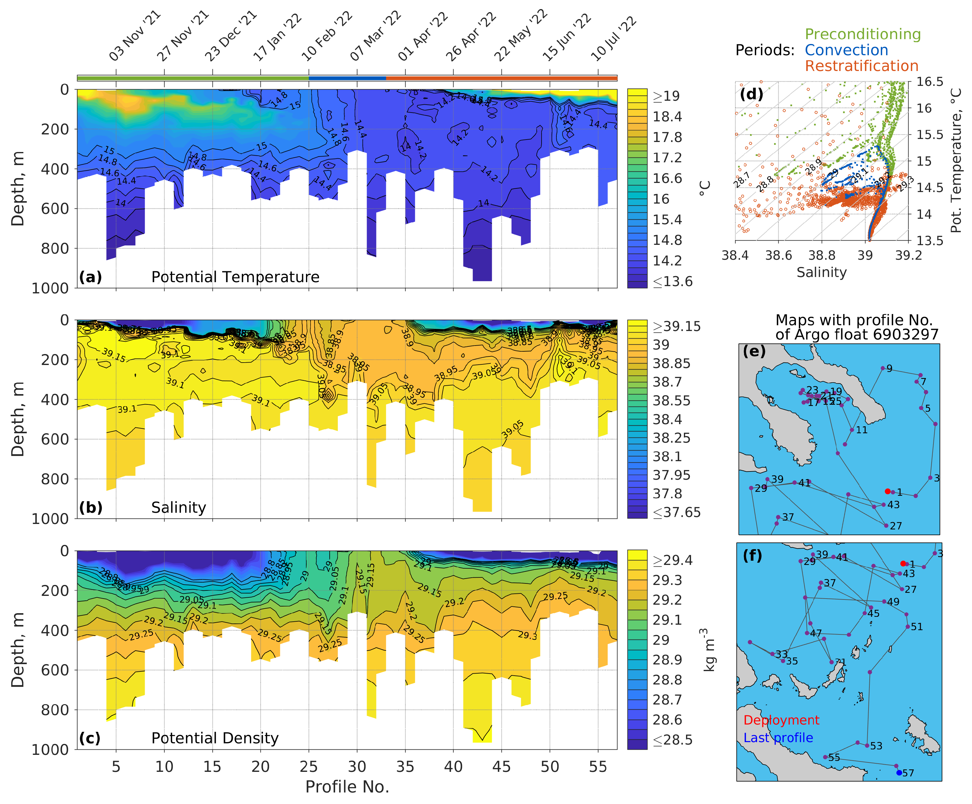
3.3. Observations from Argo Floats 297 and 298

In this section, we discuss the evolution of the NCAeg DWF during the winter of 2021–2022 using the hydrographic observations and the trajectories of floats 297 and 298.
Float 297 was deployed in the Central Athos Basin on 17 October and followed a cyclonic path towards Mount Athos, which it entered on 13 December the Singitic Gulf and remained trapped for about two and a half months (Figure 6). The upper and intermediate layers of the water column in the Central Athos Basin were occupied by LSW and LIW ( S > 39.1 ), except for a ∼ 20   m surface layer where the modified BSW was observed ( 37.5 < S < 39 , 18.5   ° C < θ < 19.5   ° C ). At the northeastern part of the Athos Basin, the BSW signal was stronger; a fresher ( 36.5 < S < 37.5 ) and colder ( 16.5   ° C < θ < 18.5   ° C ) surface layer of ∼ 50   m occupied that region. As is expected from the general circulation in the area, which is also evident by the trajectory of the float, the surface and intermediate water masses inside the Singitic Gulf were a mixture of LSW, LIW, and BSW, with the θ and S values ranging between those of the three above-mentioned water types. In the Singitic Gulf, float 297 recorded the gradual deepening of the modified BSW layer from ∼ 50   m to ∼ 150   m . The drop in temperature and increase in salinity of the modified BSW layer during the autumnal period is indicative of its transformation due to surface heat loss and vertical mixing with the underlying saltier layer. It also implies that the change in salinity of the BSW is controlled mostly by mixing with surrounding and underlying water masses rather than surface transformation due to evaporation. The minor role of evaporation in the increase in the BSW salinity will be discussed in Section 3.5.
By the end of January, the 28.9   kg m 3 isopycnal had outcropped at the surface, and the mixed layer had become deeper than 150 m . Based on the isotherms, isohalines, and isopycnals of the θ / S diagram, 28.9   kg m 3 has been previously used as the lowest density threshold for the Aegean Sea intermediate water [87]. The cores of the main intermediate water masses in the SAeg, i.e., the LIW and the CIW, were measured between 29   kg m 3 and 29.05   kg m 3 , whilst the 28.9   kg m 3 density was closer to the subsurface layer where the MAW is present. The selection of a single density threshold for the identification of intermediate water in the Aegean Sea is not straightforward, as water with even lower densities would be considered to be subducted after the convective period due to its capping by BSW in the North Aegean. Anyway, by 15 February, the density inside the ∼ 200   m mixed layer was higher than 29   kg m 3 , and in the next cycle, the float exited the Singitic Gulf. The float spent the convective period from 15 February to 1 April in the western part of the Athos basin between the Sporades Islands and the southern Chalkidiki Peninsula, thus recording mixed layer densities between 29   kg m 3 and 29.18   kg m 3 . The highest near-surface densities (∼ 29.18   kg m 3 ) were recorded only at the peak of the convective period around 20 March, and the irregular motion of the float during that period points to the breaking of the geostrophic circulation that was occurring. Subsurface water with a density of ∼ 29.15   kg m 3 and a salinity slightly higher than the one observed in the upper layer of Athos Basin during the convective period (S∼39 instead of 38.9 < S < 38.95 ) already recorded by 7 March suggests the presence of a mixture of water transported from the southern part of the NCAeg. The properties of the water formed in the Athos Basin in the 29 kg m 3 29.18   kg m 3 density range by open-sea convection were 14.2   ° C < θ < 15.1   ° C and 38.85 < S < 38.95 . The cold and relatively brackish ( S < 38.95 , θ < 14.2   ° C ) patches observed in the subsurface layer and down to a depth of 400 m were probably formed above the shallower parts of the northwestern Aegean shelves and ended up in the Athos Basin [150,151,152].
Convection ceased around 25 March. The layer defined by the 29 kg m 3 and 29.25   kg m 3 isopycnals in the Athos Basin was ∼ 170   m thick before the convective period, and it was ∼ 350   m in thickness on 1 April right after the capping of the area by a thin layer of BSW. By the end of April, the 29.25   kg m 3 isopycnal in the Central Athos Basin had risen well above the sill depth (300 m ); water with S > 39.05 , θ < 14.2   ° C , and σ θ > 29.3   kg m 3 , which was formed to the south of the thermohaline front over the Lemnos Plateau (see Section 3.4), filled the 400–700 m horizon. Float 297 exited the Athos Basin on 15 June and followed a predominantly southward path between the Skiros and Sporades Islands. On its exit, it recorded a water mass of higher temperature and salinity, therebyindicating the area between the Agios Efstratios and Sporades Islands as a confluence region for the dense water formed in different parts of the NCAeg.
Float 298 was deployed in the Lesvos Basin on 13 November and spent most of its time there moving in the deep eastern and shallow northwestern parts of the basin until its final exit on 23 February towards the Lemnos Plateau (Figure 7). A close-up bathymetry around the Lesvos Island is shown in Figure S8 to help understand the impact of topographic steering on the motion of the float. In October, warm and saline water ( S > 39.15 , θ > 18   ° C ) occupied the above sill (< 200   m ) layer, while colder but equally saline water, probably formed locally the previous year, was present below the sill depth. From the beginning of December to the end of January, a gradual deepening of the 29   kg m 3 isopycnal from 200 m to 300 m was observed, and it was accompanied by the cooling ( θ from 18 ° C to < 16   ° C ) and salting (S from > 39.15 to > 39.2 ) of the water laying above the depth of that isopycnal. The outcropping of the 29   kg m 3 isopycnal by the first days of February, along with the increase of near-surface salinity, indicate that, compared to the northern part of the NCAeg, the atmospherically driven water mass transformation was more effective around Lesvos Island.
Water with a density of 29.15   kg m 3 filled the deep pit of the Lesvos Basin below 500   m during November 2021. The highest density inside the pit were recorded on 19 January about two weeks before the surfacing of the 29   kg m 3 isopycnal, which had dropped to 29.1   kg m 3 , thereby indicating a downward buoyancy flux that is typical of the stagnation periods in deep basins [153] during that period. The near-surface density recorded by float 298 after 19 January, while outside the pit but still in the southern Lesvos region, never exceeded the 29.1   kg m 3 threshold. Thus, the appearance of a gradually increasing volume of near-bottom water with a density of > 29.15   kg m 3 should be attributed to the production of dense water in the shallower areas around Lesvos Island. Indeed, such near-surface densities were recoded by the float to the west of the Lesvos Island after definitively leaving the Lesvos Basin.
The densest near-surface water ( 29.25   kg m 3 < σ θ < 29.32   kg m 3 ) was measured from 10 to 20 March between the northern Lesvos Island and the southern Lemnos Plateau. Its thermohaline properties were 39.15 < S < 39.25 and 14.6   ° C < θ < 15   ° C . Three distinct water masses with σ θ > 29.3   kg m 3 could be distinguished in the Skiros Basin and its northeast extension by the measurements of float 298 during March and April. The first was the near-surface water mentioned above. The second was a water mass with measurements of S 39.15 and θ < 14.4   ° C , which was probably formed over the central part of the Lemnos Plateau, as its relatively low temperature and salinity should be the result of mixing of the LSW and LIW with the BSW on the south side of the thermohaline front. This explanation is also supported by the weak BSW signal recorded by float 298 while flowing westwards from the north Lesvos Island towards the Sporades Islands; the BSW signal became much stronger between the Agios Efstratios and Sporades Islands (see profile number 33 in Figure 7). The third and densest ( σ θ > 29.35   kg m 3 ) water mass of the three was saltier ( S > 39.2 ) and slightly warmer ( 14.4   ° C < θ < 14.5   ° C ) than the water mass formed over the Central Lemnos Plateau but colder than and of similar salinity to the water mass formed over the southern Lemnos Plateau, and, as will be shown in Section 3.4, it was formed to the east of the Lesvos Island.
The 29   kg m 3 isopycnal in the North Skiros Basin had risen to ∼ 60   m after the convective period. The bulk of the water produced in the southeastern part of the NCAeg was between 29.2   kg m 3 and 29.35   kg m 3 , with values of S > 39 and θ > 14.4 . By the beginning of May, float 298 had reached the Sporades Islands and followed a southward direction from there. In the west coast of the NCAeg, the layer below 200 m was occupied by the warm and saline water formed in the southeastern part of the NCAeg. The patches of colder and fresher water and the consequent higher hydrographic variability of the shallower layer in the west coasts of the NCAeg reflect the coexistence and mixing of water masses formed in other parts of the basin. By late June, both floats had converged in the southwestern coasts of the NCAeg, between the Evia and Skiros Islands, as a manifestation of the general cyclonic circulation of the region and the dispersion of newly formed water. Float 297 exited the Athos Basin in mid-June, while float 298 had been recording the colder and fresher patches in the < 200   m layer at least one and a half months earlier in this region. Thus, taking into consideration the > 200   m drift depth and the grounding of the floats, it is not clear whether the water masses observed just after the end of the convection period were formed in the northern parts of the NCAeg shelf or along the thermohaline front. According to the model’s distribution of the surface density (see Section 3.4), water with > 29   kg m 3 had not been produced in the Thracian Shelf, thus leaving the Thermaikos Gulf and the western part of the Athos Basin as the most probable formation sites, possibly with contribution from the North Evia Gulf.
From the two Argo floats deployed in the region, it can be seen that the volume of water with a density > 29.3   kg m 3 produced in the NCAeg was sufficient to uplift the 29.25   kg m 3 isopycnal above the sill depth in the Athos Basin and that a thin bottom layer with a density > 29.25   kg m 3 was overflowing from the northern parts of the NCAeg, which was moving inside the S. Skiros–Psarra Basin.

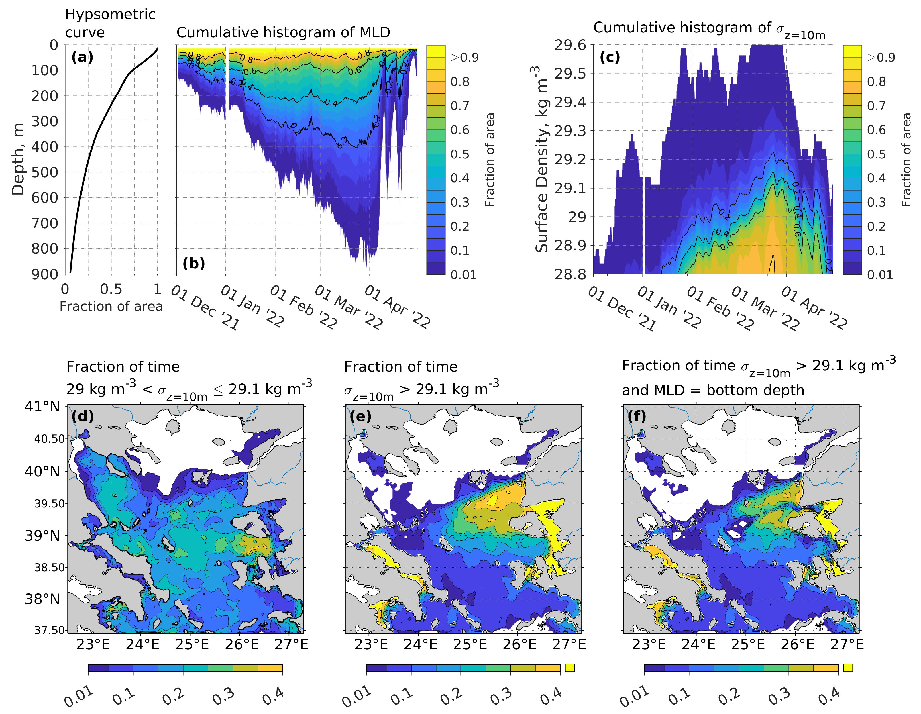
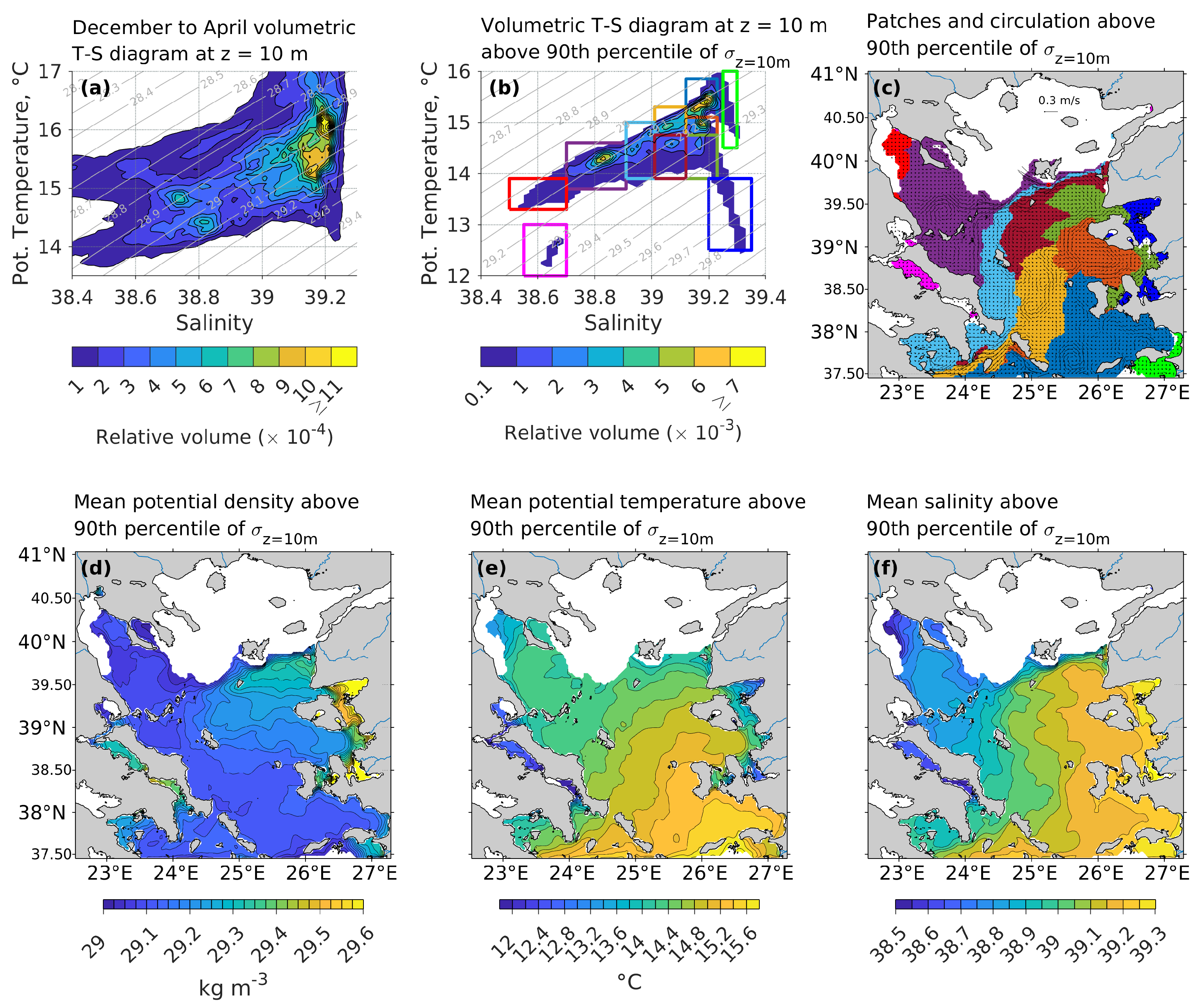
3.4. DWF Evolution from Model Output

To describe the evolution of DWF from the model, we used the two-hour output to calculate the cumulative histograms of the MLD and potential density at 10 m in depth, which was normalised by the number of wet grid points (Figure 8b,c). At every 2 h time step of the model output, the cumulative histograms show the fraction of the total area for which the various MLD and potential density values were observed. To obtain an understanding of the spatial variability of the dense water formation, we calculated at each grid point the fraction of time for which the density at the 10 m depth was between 29 kg m 3 and 29.1   kg m 3 (Figure 8d), as well as the fraction of time for which the density was higher than 29.1   kg m 3 (Figure 8e). The hypsometric curve, which refers to the proportion of land area at various elevations, is shown in Figure 8a in order to infer the spatial extent of the convective events.
The variability of the mixed layer from the beginning of December to the last week of March consisted of a gradual deepening, which followed the low-frequency variability of the buoyancy loss and several more abrupt deepenings on days of strong northerly winds, which were also the days of the strongest buoyancy loss, as discussed in Section 3.2. A wind stress magnitude above 0.5   N m 2 was accompanied by the abrupt deepening of the mixed layer around 18 December and 13 and 26 January. On the contrary, the MLD shoaled during prolonged periods of calm weather conditions, i.e., from 19 December to 28 December and from 15 February to 20 February. Before mid-January, the MLD was ∼ 140   m over 40% of the NCAeg surface area. After the two periods of harsh weather conditions during January, the MLD had become > 200   m over 40% and > 300   m over 20% of the NCAeg surface area, respectively. The mixed layer reached depths between 700 m and 800 m around 20 March when the densest water was formed. During that period, water denser than 29.1   kg m 3 covered 60% of the NCAeg area, while the production of the densest water ( σ θ > 29.25   kg m 3 ) remained localised, thereby occupying 15% of the NCAeg area. The temporal evolution of the near-surface density and MLD bore a very close resemblance throughout the period of study. By the first ten days of April, the water column had become stratified again, mostly due to the capping by the BSW and the development of a thin near-surface layer of higher temperature, and it had come very close to the state it had been in in the beginning of December in terms of the MLD. However, in terms of the surface density, the water column remained close to the state it had been in in late February, as water with σ θ > 29   kg m 3 occupied ∼ 30 % of the NCAeg area. Consequently, the two periods of moderate wind stress and relatively low air temperature centred around 7 and 18 April resulted in a sharp increase in the MLD and surface density, the extending the DWF until late April between the islands of Lesvos, Lemnos, and Skiros.
The formation of water with σ θ > 29   kg m 3 took place over a period of one to two months and over most of the NCAeg, except for the region to the north and west of the Lemnos Island, which was directly influenced by the BSW and lasted longer than a month to the south of the Lesvos Island around the Skiros Island and in the western part of theAthos Basin and Thermaikos Gulf. The formation of water with σ θ > 29.1   kg m 3 took place between the Islands of Lemnos, Skiros, and Chios, and it lasted for about one and a half months or more to the north of the Lesvos Island. The formation lasted for more than two months in the shallow areas of the Candarli Shelf, Edremit Gulf, and Smyrni Gulf. Similarly, measured values of σ θ > 29.1   kg m 3 outcropped for more than two months in the North and South Evia Gulfs, as well as in the West Saronikos Gulf. According to the model, water exported from North Evia Gulf had a limited but traceable impact to the south of the Sporades Islands. Part of the subsurface hydrographic variability in this region, as recorded by the two Argo floats, might have come from the outflow of the North Evia Gulf; however, the lack of observations in the gulf prevents further investigation. Any dispersion signal of water formed in the West Saronikos Gulf and the South Evia Gulf was masked by the water formed to the east of the Cyclades Plateau.
The fraction of time for which the surface density was higher than 29.1   kg m 3 and the MLD reached the bottom is shown in Figure 8f. The comparison of Figure 8e with Figure 8f reveals two regions: one to the north and one to south of the Lesvos Island, where the MLD did not reach the bottom even when the surface density was > 29.1   kg m 3 . The comparison suggests that the densest water produced to the northeast of the Lesvos Island and on the south part of the Lemnos Plateau ended up in the Skiros Basin as a bottom current flowing inside the trough, which constitutes the northeast extension of Skiros Basin. Similarly, part of the water produced on the Candarli Shelf filled the Lesvos Basin, while part of it flowed northwards towards the Lesvos Strait and Edremit Gulf, thus further increasing the density of the water forming there [88,89]. This is supported by the consistency of the thermohaline properties of the densest waters ( σ θ > 29.3   kg m 3 ) recorded by float 298 and the spatial distribution of the highest surface densities from the model. It is also consistent with the literature, which identifies the Skiros Basin as a rapidly responding basin that accommodates the densest and by far saltiest waters observed during the EMT [87,112,154,155].
To obtain an overview of the hydrography changes induced by DWF, we calculated the temperature, salinity, and depth of the 29.1   kg m 3 isopycnal during the first two weeks of December and the last two weeks of April (Figure 9). During the first half of December, the 29.1   kg m 3 isopycnal was deeper in the southeastern part of the NCAeg and shoaled towards the northwest. It was found at > 400   m in depth at the North Ikaria–Chios Basins, at ∼ 350   m at the Lesvos and South Skiros–Psarra Basins, and at ∼ 250   m in depth at the Skiros, Athos, and Lemnos Basins. Although a meridional gradient of the thermohaline properties of the 29.1   kg m 3 isopycnal was also present during December, the high temperature and salinity values at the east coasts of the NCAeg, along with the protrusion of the 15 ° C isothermal and the 39.1 isohaline, indicate a somewhat isotropic spreading of water from regions around the Lemnos and Lesvos Islands towards the rest of the NCAeg. However, judging from the thermohaline distribution, the progression of these warm and saline waters towards the Athos and Lemnos Basins was allowed mainly through the Agios Efstratios and Sporades Islands. The warmer and saltier water flowed along the isobaths from the Agios Efstratios Island around the northern part of the Lemnos Plateau towards the Lemnos Basin, while the colder and fresher water of the Athos Basin flowed from the eastern flank of the Sporades Islands parallel to the Evia Island and towards the Cyclades Islands.
During the second half of April, the 29.1   kg m 3 isopycnal has been uplifted at < 50   m in depth between the Lemnos, Skiros, Chios, and Lesvos Islands and at ∼ 200   m in depth at the Athos and Lemnos Basins. The thermohaline distribution on the 29.1   kg m 3 isopycnal illustrates, on the one hand, the formation of water over the southeast part of the NCAeg, which was covered by LSW, and, on the other hand, the formation of water near the BSW–LSW front where the BSW diluted and cooled the near-surface water. The dispersion of the recently formed water can be inferred by the depth and the thermohaline properties of the 29.1   kg m 3 isopycnal, as its gradual deepening to the western and southern regions of the NCAeg, along with the southwestward extension of the less spicy water, clearly indicates the dispersion of the recently formed water towards the SAeg through the Mykonos–Ikaria Strait. The steeper SE–NW gradient of the 29.1   kg m 3 isopycnal depth, which extended from the Dardanelles Strait to the Sporades Islands and then turned parallel to the west coasts of the NCAeg, matches the thermohaline gradient and indicates the location of the thermohaline front and the cyclonic circulation of the region.
An analysis of the surface water types and water masses from the model output is shown in Figure 10. To identify the properties of the densest water produced in the NCAeg, we marked the highest 10% surface density values at each grid point, which correspond roughly to a period of two weeks, and conducted a θ / S analysis only during that period (Figure 10b). Also, only the grid points whose 90th percentile of surface density was above 29   kg m 3 were included in the analysis. The spatial distribution of the water masses of Figure 10b is shown in the map of patches in Figure 10c, and their thermohaline properties are shown in Figure 10d–f. The θ / S diagram from December to April is shown for reference in Figure 10a.
LSW and BSW, the two main water masses occupying most of the surface area of the NCAeg from December to April, can be distinguished in the volumetric θ / S diagram at 10 m depth (Figure 10a). The LSW, with 15.5   ° C < θ < 16.5   ° C and 39.1 < S < 39.25 , was the most abundant water mass, while the properties of the bulk of modified BSW were between 14   ° C < θ < 15   ° C and 38.7 < S < 38.85 . From the θ / S diagram containing only the highest 10% of the density values and the map of patches, it can be seen that the LSW, which entered the NCAeg from the southeastern boundary, was transformed by surface heat loss on its way towards the Lemnos Plateau while retaining its high salinity signature along its main pathway. When it reached the northern part of the Lesvos Island, its temperature was very close the temperature of the south side of the thermohaline front, but its salinity was much higher. There, it mixed laterally with the modified BSW, thereby creating a water mass with a temperature of ∼ 14.5   ° C , a salinity of 38.9 < S < 39.2 , and a density of 29.1   kg m 3 < σ θ < 29.35   kg m 3 , and it recirculated to the east of the Skiros Island and along the central meridional axis of the NCAeg. The properties of the modified BSW with σ θ > 29   kg m 3 were set in the middle of the Lemnos Plateau between the Lemnos and Tenedos Islands from where it spread westwards and covered the Sporades Islands and the deep part of the Athos Basin. The North Cyclades Plateau was a confluence region of three water masses. The first was a warm and saline westward extension of the LSW. The second and third water masses were a mixture of BSW and LSW, as they both laid on a straight line connecting the BSW and LSW in the θ / S diagram. The properties of the second water mass were set in the central part of the southern NCAeg. It contained a higher amount of LSW and flowed towards the Myrtoan Sea through the North Cyclades Plateau. The third water mass, which contained a higher amount of BSW, was formed close the to the thermohaline front over the Lemnos Plateau, and from there it was rapidly advected to the North Cyclades Plateau through the Kafireas Strait and filled the Saronikos Gulf. The resulting dense water mass formed over the North Cyclades Plateau ( σ θ 29.2   kg m 3 ) was warmer and saltier than those flowing parallel to the Evia Island and entering through the Kafireas Strait.
The surface heat loss of LSW and its progressive mixing with the modified BSW also determined the spatial distribution of the surface open-sea hydrographic properties of the NCAeg to the south of the thermohaline front. The surface density became higher along the east coasts of the NCAeg from the latitude of the Chios Island to the latitude of the Lemnos Island due to surface heat loss, while the salinity remained almost constant. Thus, north of the latitude of the Chios Island, the gradient of the surface salinity retained its stronger zonal component, while the direction of the surface temperature gradient progressively became meridional. Below the latitude of the Chios Island, the horizontal gradient of both the temperature and salinity had a stronger zonal component, which was parallel to the elongated patches, thereby indicating that the lateral mixing of LSW and modified BSW was the dominant process there.
Four dense coastal water masses could be identified in addition to the aforementioned open-sea ones. The central part of the southern Thermaikos Gulf was covered by a water mass, which resulted from the mixing of BSW with the riverine input to the north and west of the gulf. The encirclement of water by land inside the North Evia Gulf and the minor exchange with the open sea resulted in a very cold water mass ( θ < 13   ° C ) despite the mild surface heat loss over the gulf. Its salinity (S 38.65 ) was marginally lower than that of the modified BSW, which covered the northwest part of the NCAeg due to the input of the Spercheios river. The other two dense coastal water masses were formed at the east coasts of the NCAeg (in Kusadasi, Izmir and Edremit Gulfs, the shelf of Candarli, and Lesvos Strait) and were characterised by lower temperature and higher salinity values compared to the formed open-sea dense water of the southeast NCAeg due to atmospherically driven transformation. Of particular interest is the coastal region to the north of the Chios Strait, as the densest water of the NCAeg ( σ θ > 29.4   kg m 3 ) was formed there, and not only filled the surrounding depressions as a bottom current but also contributed to the increase in surface density between the Lesvos and Lemnos Islands where the bulk of dense water with σ θ > 29.2   kg m 3 was produced.

3.5. One-Dimensionality of the Water Column

The formation of dense water in the NCAeg is an interplay between the lateral advection of two distinct water masses, thereby involving their mixing and their atmospherically driven transformation. The inflow of BSW reduces air–sea interactions and adds an amount of buoyancy, which almost compensates for surface freshwater loss [143]. The inflow of LSW brings saline water over the shallow regions of the eastern coasts of the NCAeg where they are subjected to intense transformation through surface buoyancy loss. Here, we used the model output to assess the extent to which surface fluxes caused the change in heat, salt, and buoyancy content in the full-depth water column and inside the mixed layer, i.e., we quantified the one-dimensionality of the water column.
The time-mean and field-mean ratios of the temporally integrated surface fluxes to the mixed layer and the full-depth water column content change are shown in Figure 11. As expected, the surface heat flux explained a higher percentage of heat content change close to the coast and over the shallow regions (> 40 % ) compared to the deeper open-sea regions of the NCAeg, while in enclosed gulfs and over the shelves, it explained > 60 % and up to 80% of the heat content change. Both the mixed layer and the full-depth heat content change had the same sign with the surface heat flux over all of the NCAeg, even above the deepest regions where their ratios were very close to zero. As can be seen by the almost random spatial distribution of the freshwater ratio between 5 % and 5 % , the surface freshwater flux had a negligible contribution to the salinity change over most of the NCAeg, with a few notable exceptions, namely, the eastern coastal areas where the densest water was formed, the eastern part of the outer Thermaikos Gulf, the Saronikos Gulf, the Pagasitikos Gulf, and the North and South Evia Gulfs. However, owing to the BSW inflow, the mixed layer freshwater ratio over the Lemnos and Athos Basin was slightly lower compared to the southern regions. This small north-to-south difference was enough to flip the meridional distribution of the mixed layer buoyancy ratio; the lower values of the heat ratio were found over the deep regions to the south of the Skiros Island, whilst the lower values of the buoyancy ratio were found over the deep regions to the north of the Sporades and Lemnos Islands. Also, in general, the deeper the water column, the lower the full-depth heat ratio was, with two notable exceptions where the ratio was disproportionally low with respect to the depth. The first was the Musellim Strait from where very dense water flowed inside the Skiros Basin, and the second was the Kafireas Strait from where the modified BSW entered the Myrtoan Sea. In both cases, strong currents were present due to topographic constraints.
Considering the temporal variability of the field-mean ratios, the heat content change explained by the surface heat flux varied from ∼ 10 % during periods of mild heat loss to ∼ 60 % during periods of strong heat loss. Since the heat flux controlled the net buoyancy flux, the range and temporal variabilities of the buoyancy ratio were almost identical to the heat ratio. The temporal variability of the freshwater ratio was mostly similar to that of the heat ratio, but its maximum value was < 15 % . From the beginning of December to around 25 March, i.e., the period when the NCAeg lost buoyancy to the atmosphere, the field-mean freshwater ratio was positive. From the last days of March to the end of April, with the exception of the two episodes of northerly winds, which were discussed in Section 3.4, the NCAeg gained buoyancy. During that period, the field-mean freshwater ratio became practically zero due to mild wind conditions and the increase in air temperature, which significantly reduced the E P (Figures S4 and S7), as well as the increased BSW inflow, which followed the mid-March DWF. Also, the mixed layer ratios were slightly higher than the full-depth ratios. The largest differences were observed from December to February, before the deepening of the mixed layer below 400 m , and from the end of March, when the restratification period began, to the end of April.

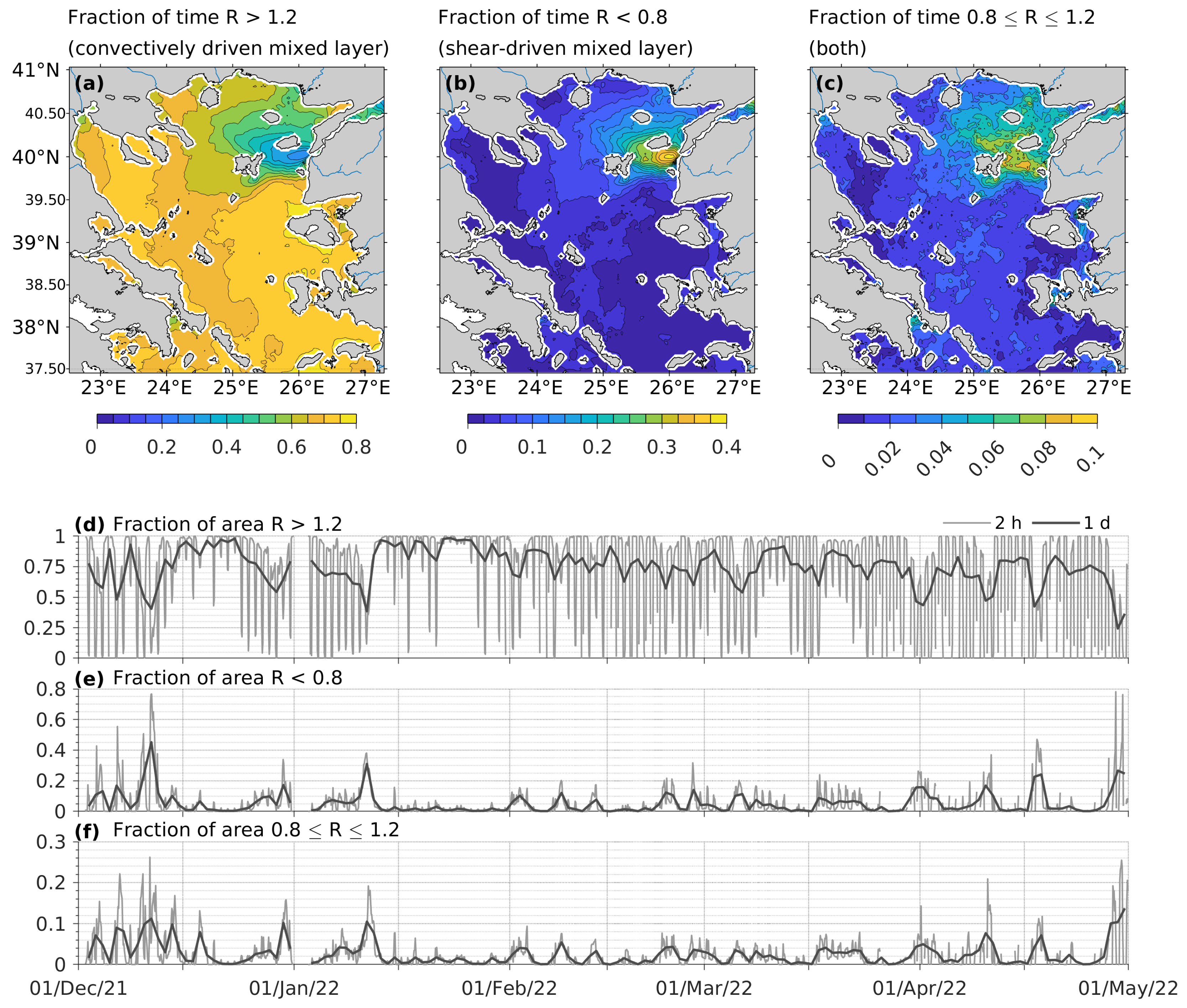
3.6. Turbulence inside the Mixed Layer

The mixed layer deepened mostly during strong and cold northerly winds, which were also the conditions of intense buoyancy loss. Thus, it is not clear whether the turbulence inside the mixed layer was buoyancy- or shear-driven. A description of the relative importance of the forced and free convection is given here using Equation (7) (Section 2.3).
Buoyancy loss to the atmosphere was the main driver of deepening of the mixed layer over most of the surface area of the NCAeg, as R > 1.2 for at least three months out of the five month simulation (Figure 12). The highest contribution of the buoyancy loss was observed over the southeastern part of the NCAeg and the western part of Athos basin. The contribution of wind was comparable to that of the buoyancy loss only in the northeastern part of the NCAeg, around the Imbros, Samothraki, and Lemnos Islands, i.e., along the main spreading pathway of the BSW. Wind was dominant only for about two weeks at the Dardanelles exit and for a few days throughout the rest of the NCAeg. However, the MLD was shallow in the areas where wind contributed significantly, and no DWF took place there. The prevention of the deepening of the mixed layer through the decrease in the buoyancy loss due to the BSW is illustrated in Figure 12a. From mid-January to the end of March, the wind contribution was restricted to over < 20 % of the NCAeg surface area mainly between the Dardanelles exit and the Thracian Shelf. Wind played a significant role to the deepening of the mixed layer depth during the first two weeks of December, which was when its contribution was comparable or higher than that of the buoyancy over half of the surface area of the NCAeg. Wind contribution to the deepening of the mixed layer was also above average during the two episodes that took place around the 7 and 18 April (see Section 3.4).

3.7. Export of Dense Water towards the SAeg

According to the model results, until the end of April, the highest density exported towards the Myrtoan Basin through the Kafireas Strait and towards the Cretan Sea through Mykonos–Ikaria Strait was < 29.2   kg m 3 . Float 297 exited the model’s domain in April 2023 (no DWF was recorded in the NCAeg during the winter of 2023 by the Argo floats) through the Mykonos–Ikaria Straits towards the southeastern Aegean Sea, thereby following closely the known pathway along the eastern flank of the Cyclades Islands and into the Cretan Sea. A θ / S diagram of float 297 before and after its exit confirms that the exported density from the NCAeg to the SAeg one year after the DWF of the winter of 2021–2022 was ∼ 29.23   kg m 3 (Figure 13). Another θ / S comparison in March–April 2023 between float 297 before exiting the NCAeg and float 1902582, which was in the northern Myrtoan Sea at the time, revealed that water above 650 m with a maximum density of ∼ 29.18   kg m 3 was transported into the Myrtoan Sea from the NCAeg through the North Cyclades Plateau. In the Myrtoan Sea, the density horizons between 29.18   kg m 3 < σ θ < 29.23   kg m 3 below 650 m were occupied by a distinct water mass with properties of 39.12 < S < 39.21 and θ 14.95   ° C . The water mass in the deep Myrtoan Sea was warmer and saltier compared to water masses of similar densities north of 37.5 ° N and probably was formed over the Cyclades Plateau, since the near-surface density in the Cretan Sea during the winter of 2022 was < 29.13   kg m 3 .
During the autumn of 2021, the core of the TMW was around 1000 m in depth at the location of the E1-M3A observatory in the Central Cretan Sea. Monthly mean E1-M3A observations at 1000 m from May 2022 to July 2023 show that the potential density increased from ∼ 29.2   kg m 3 to ∼ 29.23   kg m 3 , and it can be seen that water exported from the NCAeg caused the rise in density, as the trace produced on the θ / S diagram by the progressive increase in the salinity and temperature lies on the imaginary line connecting the TMW properties before the formation with the properties of water masses exported from the NCAeg after the formation. The monthly mean densities of ∼ 29.23   kg m 3 were the highest recorded by the E1-M3A observatory since its deployment in mid-2007. However, some periods of missing data exist, of which the most interesting for DWF is from mid-2012 to mid-2013.

4. Discussion

The present study partially fills a gap in the NCAeg DWF literature after 2017. In the Athos Basin, the maximum density (∼ 29.35   kg m 3 ) and ventilation depth (∼ 700   m ) during the winter of 2021–2022 DWF were comparable to those of the last published DWF episode in the Aegean Sea in the winter of 2016–2017 [47]. The long-term salinification and warming of the near-surface and intermediate water masses of the EMed [156,157], as well as the sharp increase in the near-surface salinity in the last five years, propagated in the intermediate layers of the Athos Basin down to the maximum ventilation depth. Prior to 2017, the highest salinity waters ( 39.025 < S < 39.05 ) were found below 700 m [47]. In 2023, the highest salinity values ( S > 39.05 ) were observed in the 200–700 m layer. This increase in salinity was accompanied by an ∼ 0.15   ° C increase in temperature. The DWF of 2017 caused a drop in salinity [47], which was probably due to the penetration of the BSW layer. High salinity below the sill depth prior to the 2022 formation implies that at least another DWF event occurred after 2017.
The formation sites of the highest density waters in the winter of 2021–2022 were the Central and Southern Lemnos Plateau and the shallow coastal regions to the east of the Lesvos Island, which are in agreement with the literature [6,87,89]. Open-sea convection took place in the southern and central parts of the NCAeg; however, the density of water produced there was lower by 0.15   kg m 3 or more compared to the shallow regions. The cyclonic circulation of newly formed water, which has been shown previously through the analysis of model output [151], was observed directly by deep-drifting floats for the first time by the present study. Although a qualitative representation of the dispersion of dense water inside the Aegean Sea exists in the literature [158,159], a quantitative time-dependent depiction of its variability and of the processes involved is still missing. Also, bottom currents, which are clearly important for the dispersion of dense water in Aegean Sea, are more appropriately represented in nonhydrostatic models [160,161]; however, no such models have been implemented so far in the region.
Either excessive single-year DWF (e.g., 1987) or successive years of DWFs of sufficient volume (e.g., 1992–1993) can result in the accumulation of dense water and, consequently, the interannual shoaling of isopycnals in the Aegean Sea, which in turn intensify the formation of the follow-up years by the outcrop of isopycnals of higher density [7,89]. The 29.1   kg m 3 isopycnal before the 2021–2022 formation was at ∼ 300   m to the north of the Skiros Island, and deeper in the North Ikaria–Chios and South Skiros–Psarra Basins. For reference, the 29.1   kg m 3 isopycnal in the Athos Basin during September 1988, after the DWF of 1987, was found at 150   m . It appears that no DWF events from 2017 onwards were sufficiently strong to trigger such a process that would enhance the DWF in the winter of 2021–2022. However, reduced residence time due to the geostrophic response of the Aegean Sea to the Etesian winds is another factor that could play a role [108].
From a climatological point of view, a comparison of the winter surface density fields of the MEDATLAS and Mediterranean Sea Hydrographic Atlas [162,163] (Figures S10 and S11) reveals a difference in the location of the formation sites between the two climatologies. The main DWF site in the MEDATLAS climatology is located over the Lemnos Plateau but confined to the north and west of the Lesvos Island. The main DWF site in Mediterranean Sea Hydrographic Atlas, on the other hand, has shifted to the south, between the Chios and Lesvos Islands, and includes the region to the east of the Lesvos Island. Our results agree with MEDATLAS regarding the Lemnos Plateau and with the Mediterranean Sea Hydrographic Atlas regarding the eastern shallow coasts. Putting extra effort into observing the shallow coastal parts of the southeastern NCAeg seems justified, as they play a significant role but remain relatively undersampled compared to other key regions for DWF in the Aegean Sea.
In the last decade, Argo profiles have been by far the most abundant source of hydrographic observations in the Aegean Sea. Argo floats are designed to operate in the deep ocean, not in shallow areas with complex topography. The activities of the Euro-Argo Research Infrastructure community for the deployment of Argo floats in shallow, coastal areas of the Mediterranean Sea have contributed significantly to the monitoring of the NCAeg [164]. Still, the scarcity of coastal shallow water observations (<∼ 300   m ) in the eastern and northern periphery of the NCAeg, as we noted from the distribution of available data in the World Ocean Database and SeaDataNet Aggregated Datasets until July 2023, poses an important limitation for current and future studies of the Aegean Sea. The difference in the stations’ spatial distributions in the inset maps of the NCAeg in Figure 3 is indicative of the issue. The BSW, which affects surface fluxes [7,142,143], disperses in the Aegean Sea along the northern periphery of the NCAeg, while the highest density waters in the Aegean Sea have been observed in the eastern periphery of the NCAeg [89]. Also, the dependence on only one platform is not an optimal observing strategy. Apart from the lack of independent observations required for the validation of data-assimilating models, Argo floats, such as any platform, have their own disadvantages; e.g., the conductivity cell sensor drift, which is the most significant source of salinity error, increases as the deployment duration of Argo floats becomes longer. The magnitude of the recent global-scale positive salinity bias (peaking in 2017–2018), which has been identified in hydrographic observations of Argo floats (< 0.025 in the EMed) [165], was not large enough to mask the near-surface and subsurface salinification signal (> 0.05 in the EMed according to the CORA gridded product, which incorporates Argo floats), but an overestimation should be expected in Argo-based representations of the EMed salinity. The shortage of independent long-term observations is amplified in the NCAeg due to last year’s shrinking of POSEIDON’s observing network, which interrupted the longest fixed-point open-sea marine and atmospheric records in the region.
The direct input of buoyancy and the reduction in air–sea interactions due to the BSW inflow, also considering that the NCAeg convection is primarily buoyancy-driven, is important both for the short-term and for the interannual variability of DWF in the NCAeg [7,143]. To date, however, continuous, long-term, and open-access information of the exchange between the Aegean and Black Seas through the Turkish Straits System (TSS) is unavailable. According to our judgement, modelling efforts for the connection of the two basins and the parameterisation of the exchange have solved the problem only partially (our model included); the performance of models in the NCAeg still falls behind compared to that in the SAeg and other regions of the EMed. Exchange through the TSS is becoming ever more important as the ongoing warming and salinification of the EMed raises the question regarding the future of its overturning circulation and the impacts on the ecosystem [77], and models’ refinements will benefit significantly from such information. For the time being, the sustained deployment of Argo floats in the NCAeg is crucial both for the short-term prediction of the Aegean Sea through regional- and basin-scale data-assimilating models and for the evaluation of nonassimilating long-term simulations related to climatic studies.

5. Conclusions

Water with density > 29.3   kg m 3 was produced in the central and eastern regions of the NCAeg and filled the intermediate layer (400– 700 m ) of the Athos Basin. The volume of dense water produced was enough to uplift the 29.1   kg m 3 isopycnal from ∼ 400   m to < 100   m over most of the NCAeg and to < 200   m over all of the NCAeg. The main region of DWF was located between Lemnos, Skiros and Lesvos Islands, and in the eastern coasts of the NCAeg to the east of Lesvos Island. The intense atmospherically driven water mass transformation (both thermal and saline) of waters of Levantine origin in the shallow region to the east of the Lesvos Island produced waters with extremely high density (> 29.6   kg m 3 ). Such densities have also been reported in the literature during the EMT but also more recently [89,166], which implies that the coastal regions to the east of the Lesvos Island have the capacity to produce extremely dense waters relatively regularly. Their volume probably depends on local atmospheric forcing [89] and background preconditioning due to the lateral transport of heat and salt from the straits. Also, part of the high-density near-surface waters in the region reached the southern Lemnos Plateau, thus contributing to the increase in density in the area. The bottom current, which flowed inside the North Skiros Basin through the Musellim Strait, might explain the fact that the North Skiros Basin has accommodated the saltiest and densest water in the Aegean Sea.
Warm and salty LSW and LIW were observed during the fall of 2021 in the central part of the Athos Basin, thus bringing high salinity water farther north than usual and indicating a reduced inflow of BSW. The high salinity of LSW and LIW (> 39.2 ) observed in the southern Lesvos region, which lies on the main pathway of waters from the Levantine Sea, is in agreement with the salinity increase in the near-surface layer of the EMed after 2015. Salinity in the intermediate layers of the Skiros Basin below the sill depth after the 2022 DWF was comparable or higher than the 39.15 value, which was observed during the EMT. However, the temperature recording in 2022 (∼ 14.5   ° C ) was much higher than in the EMT ( 13.25   ° C ). The EMed-wide increase in temperature from 2005 to 2015 prevented the production of water with higher densities, despite the strong buoyancy loss during the winter of 2022.
The buoyancy loss during the winter of 2021–2022 was comparable to that of 1993–1994, 2002–2003, and 2012, which were all years of DWF in the Aegean Sea [143]. The buoyancy loss was higher over the southeastern part of the NCAeg where LSW was present and lower almost by a factor of two over areas capped by BSW. The regions under the direct influence of the BSW did not participate in the production of dense water (surface value of σ θ < 29   kg m 3 ). Riverine discharge reduced air–sea interactions even more, especially in the coastal areas of the Thracian Shelf, the western part of the Thermaikos Gulf, and the semienclosed gulfs in the western coasts. Surface heat flux accounted for about 50 % or more of the heat content change in regions shallower than roughly 200   m . In the very shallow regions of the eastern coasts, surface freshwater flux accounted for up to 25 % of the salt content change, thus increasing the salinity of the LSW. Advection was the dominant cause of salt content change over the rest of the NCAeg, with negligible contribution from the surface freshwater flux.
The formation during the winter of 2021–2022 in the NCAeg was strong enough to affect the deep layers of the SAeg. The mixing of dense waters exported from the NCAeg with the TMW found in the SAeg resulted in the increase in temperature, salinity, and density at 1000 m in the Central Cretan Sea, as has been recorded by continuous fixed-point observations until July 2023. The density increase induced by the winter 2021–2022 formation is the largest that has been recorded in the Central Cretan Sea by the fixed-point observatory E1-M3A since 2007.

Supplementary Materials

The following supporting information can be downloaded at https://0-www-mdpi-com.brum.beds.ac.uk/article/10.3390/jmse12020221/s1. Figure S1: Time-mean and standard deviation of (a) salinity and (b) temperature profiles from Argo observations compared to the time-mean model profiles. (c) Model and observations θ / S diagram. Salinity (d) root mean square error and (e) bias profiles between model output and Argo observations. Temperature (f) root mean square error and (g) bias profiles between model output and Argo observations. Time-dependent correlation, bias and root mean square error for (h, k) salinity, (j, l) temperature, and (j, m) density, between model output and observations. (n) Number of profile observations per month. Figure S2: Spatiotemporal variability of thermodynamic properties of sea water from 2 December 2021 – 30 April 2022 over the study area. Time-mean (a) thermal expansion coefficient a, (b) saline contraction coefficient b, and (c) heat capacity C p . Field-mean (d) thermal expansion coefficient a, (e) saline contraction coefficient b, and (f) heat capacity C p . Figure S3: Spatial variability of parameters used for the calculation of thermal, freshwater and momentum surface fluxes from 2 December 2021 to 30 April 2022 over the study area. Time-mean (a) sea surface temperature (SST), (b) air temperature at 2 m height, (c) difference between SST and air temperature, (d) saturation humidity at sea surface, (e) specific humidity, (f) difference between saturation and specific humidity, (g) relative humidity, (h) wind stress magnitude and direction, and (i) cloud fraction. Figure S4: Temporal variability of parameters used for the calculation of thermal, freshwater and momentum surface fluxes from 2 December 2021–30 April 2022 over the study area. Field-mean (a) air temperature at 2 m height and sea surface temperature, (b) saturation humidity and specific humidity, (c) wind stress magnitude, (d) wind stress direction, and (e) cloud fraction. Figure S5: Time-mean surface heat flux components and net flux. (a) Shortwave, (b) net longwave, (c) sensible, (d) latent, and (e) net heat flux, averaged from 2 December 2021 to 30 April 2022. Figure S6: Field-mean surface heat flux components and net heat flux. (a) Shortwave, (b) longwave, (c) sensible, (d) latent, and (e) net heat flux, averaged over the North and Central Aegean Sea. Low-passed shortwave and net radiation is also shown. Figure S7: Time-mean and field-mean components of freshwater flux and net freshwater flux. Time-mean (a) evaporation, (b) precipitation, and (c) evaporation minus precipitation for the period 2 December 2021–30 April 2022. Field-mean (d) evaporation, (e) precipitation, and (f) evaporation minus precipitation, averaged over the North Aegean. Figure S8: A close-up bathymetry map around Lesvos Island. Figure S9: Atmospherically driven water mass transformation rates above the potential density thresholds 29, 29.1, 29.2, and 29.3   kg m 3 . Figure S10: Winter climatology of (a, b, c) potential temperature, (d, e, f) salinity, and (g, h, i) potential density from MEDATLAS at 10 m depth. Figure S11: Winter climatology of (a, b, c) potential temperature, (d, e, f) salinity, and (g, h, i) potential density from Mediterranean Sea Hydrographic Atlas at 10 m depth.

Author Contributions

Conceptualization, M.P., I.G.M., E.T. and V.Z.; methodology, M.P., I.G.M., E.T. and V.Z.; software, M.P. and I.G.M.; validation, M.P. and I.G.M.; formal analysis, M.P. and I.G.M.; investigation, M.P., I.G.M., D.K., D.B., E.T. and V.Z.; data curation, M.P., I.G.M. and D.K.; writing—original draft preparation, M.P. and I.G.M.; writing—review and editing, M.P., I.G.M., E.T., V.Z. and D.K.; visualization, M.P. and I.G.M.; supervision, E.T. and V.Z.; project administration, E.T. and V.Z.; funding acquisition, E.T. and V.Z. All authors have read and agreed to the published version of the manuscript.

Funding

The operational model was developed under the projects “Infrastructure building for Supporting Blue Growth in the North Aegean: Coastal Environment Observatory (AEGIS)” (contract MIS 5021550) and “Coastal Environment Observatory and Risk Management in Island Regions AEGIS+” (contract MIS 5047038). Argo float 298 was deployed within the framework of the project “Hellenic Integrated Marine and Inland Water Observing, Forecasting and Offshore Technology System, HIMIOFoTS” (contract MIS 5002739). Project AEGIS was funded by the Operational Programme “North Aegean 2014-2020”. Projects HIMIOFoTS and AEGIS+ were implemented within the Operational Programme “Competitiveness, Entrepreneurship and Innovation” (NSRF 2014-2020), which was cofinanced by the Hellenic Government (Ministry of Development and Investments) and the European Union (European Regional Development Fund). Both Argo float missions were part of the Euro-Argo RISE (EU H2020 programme, Grand Agreement No. 824131) project under the context of investigating the performance of Argo floats in shallow, coastal areas. M.P. was supported by YPATIA scholarships (contract No. 3030–163) through the University of the Aegean for PhD studies.

Institutional Review Board Statement

Not applicable.

Informed Consent Statement

Not applicable.

Data Availability Statement

The bathymetry data have been downloaded from EMODnet (https://www.emodnet-bathymetry.eu/, accessed on 24 January 2024) [82]. Argo data have been downloaded from Coriolis (https://0-doi-org.brum.beds.ac.uk/10.17882/42182, accessed on 24 January 2024) [97]. Argo data were collected and made freely available by the International Argo Program and the national programs that contribute to it (https://argo.ucsd.edu/data/acknowl-edging-argo, accessed on 24 January 2024). The Argo Program is part of the Global Ocean Observing System (http://0-doi-org.brum.beds.ac.uk/10.17882/42182, accessed on 24 January 2024). The gridded CORA data set has been downloaded from the Copernicus Monitoring Service (https://0-doi-org.brum.beds.ac.uk/10.17882/46219, accessed on 24 January 2024) [98]. The E1-M3A mooring observations in the Central Cretan Sea [99], which are distributed in the Mediterranean Sea In Situ Near Real Time Observations product, have been downloaded from the Copernicus Marine Service (https://0-doi-org.brum.beds.ac.uk/10.48670/moi-00044, accessed on 24 January 2024). The NAG model data are available from I.G.M. upon request.

Acknowledgments

We thank Eva Krasakopoulou for her constructive comments. We thank Panagiotis Papachiou and the IT department of the University of the Aegean for the provision of computational resources.

Conflicts of Interest

The authors declare no conflicts of interest.

Abbreviations

The following abbreviations are used in this manuscript:
BSWBlack Sea Water
CMEMSCopernicus Marine Environment Monitoring Service
DWFDense Water Formation
EMDWEastern Mediterranean Deep Water
EMedEastern Mediterranean Sea
EMTEastern Mediterranean Transient
LIWLevantine Intermediate Water
LSWLevantine Surface Water
MAWModified Atlantic Water
MLDMixed Layer Depth
NAGNorth Aegean Sea Model
NCAegNorth–Central Aegean Sea
SAegSouth Aegean Sea
SSTSea Surface Temperature
TMWTransitional Mediterranean Water

References

  1. Malanotte-Rizzoli, P.; Hecht, A. Large-scale properties of the Eastern Mediterranean—A review. Oceanol. Acta 1988, 11, 323–335. [Google Scholar]
  2. Malanotte-Rizzoli, P.; Robinson, A.R. POEM: Physical Oceanography of the Eastern Miditerranean. Eos Trans. Am. Geophys. Union 1988, 69, 194–203. [Google Scholar] [CrossRef]
  3. Georgopoulos, D.; Theocharis, A.; Zodiatis, G. Intermediate water formation in the Cretan Sea (south Aegean Sea). Oceanol. Acta 1989, 12, 353–359. [Google Scholar]
  4. Malanotte-Rizzoli, P.; Manca, B.; d’Alcala, M.R.; Theocharis, A. The Eastern Mediterranean in the 80’s and in the 90’s: The big transition emerged from the POEM-BC observational evidence. In The Eastern Mediterranean as a Laboratory Basin for the Assessment of Contrasting Ecosystems; Malanotte-Rizzoli, P., Eremeev, V.N., Eds.; NATO Science Series 2: Environmental Security; Springer: Dordrecht, The Netehrlands, 1999; Volume 51, pp. 1–6. [Google Scholar] [CrossRef]
  5. Gertman, I.; Ovchinnikov, I.; Popov, Y.I. Deep water formation in the Aegean Sea. Rapp. Comm. Int. Mer Médit. 1990, 32, 164. [Google Scholar]
  6. Theocharis, A.; Georgopoulos, D. Dense water formation over the Samothraki and Limnos Plateaux in the north Aegean Sea (Eastern Mediterranean Sea). Cont. Shelf Res. 1993, 13, 919–939. [Google Scholar] [CrossRef]
  7. Zervakis, V.; Georgopoulos, D.; Drakopoulos, P.G. The role of the North Aegean in triggering the recent Eastern Mediterranean climatic changes. J. Geophys. Res. Oceans 2000, 105, 26103–26116. [Google Scholar] [CrossRef]
  8. Yüce, H. Northern Aegean Water Masses. Estuar. Coast. Shelf Sci. 1995, 41, 325–343. [Google Scholar] [CrossRef]
  9. Krestenitis, Y.N.; Valioulis, I.A. Investigation of the deep water formation in the N. Aegean Sea basin. WIT Trans. Ecol. Environ. 1994, 8, 107–114. [Google Scholar]
  10. Roether, W.; Manca, B.B.; Klein, B.; Bregant, D. Recent changes in eastern Mediterranean deep waters. Science 1996, 271, 333–335. [Google Scholar] [CrossRef]
  11. Theocharis, A.; Klein, B.; Nittis, K.; Roether, W. Evolution and status of the Eastern Mediterranean Transient (1997–1999). J. Mar. Syst. 2002, 33–34, 91–116. [Google Scholar] [CrossRef]
  12. Zervakis, V. Ocean Obs: Mediterranean circulation and thermohalne functioning during the instrumental period. In Proceedings of the International MedCLIVAR-ICTP-ENEA Summer School on the Mediterranean Climate System and Regional Climate Change, Trieste, Italy, 13–22 September 2010; pp. 1–14. [Google Scholar]
  13. Lascaratos, A.; Roether, W.; Nittis, K.; Klein, B. Recent changes in deep water formation and spreading in the eastern Mediterranean Sea: A review. Prog. Oceanogr. 1999, 44, 5–36. [Google Scholar] [CrossRef]
  14. Drakopoulos, P.; Lascaratos, A. Modelling the Mediterranean Sea: Climatological forcing. J. Mar. Syst. 1999, 20, 157–173. [Google Scholar] [CrossRef]
  15. Korres, G.; Lascaratos, A. A one-way nested eddy resolving model of the Aegean and Levantine basins: Implementation and climatological runs. Ann. Geophys. 2003, 21, 205–220. [Google Scholar] [CrossRef]
  16. Triantafyllou, G.; Korres, G.; Petihakis, G.; Pollani, A.; Lascaratos, A. Assessing the phenomenology of the Cretan Sea shelf area using coupling modelling techniques. Ann. Geophys. 2003, 21, 237–250. [Google Scholar] [CrossRef]
  17. Nittis, K.; Lascaratos, A.; Theocharis, A. Dense water formation in the Aegean Sea: Numerical simulations during the Eastern Mediterranean Transient. J. Geophys. Res. Oceans 2003, 108, 8120. [Google Scholar] [CrossRef]
  18. Ilyin, Y.P.; Lemeshko, E.M.; Stanichny, S.V.; Soloviev, D.M. Satellite observations of similar circulation features in semi-enclosed basins of the Eastern Mediterranean with respect to marine ecosystems investigations. In The Eastern Mediterranean as a Laboratory Basin for the Assessment of Contrasting Ecosystems; Malanotte-Rizzoli, P., Eremeev, V.N., Eds.; NATO Science Series 2: Environmental Security; Springer: Dordrecht, The Netherlands, 1999; Volume 51, pp. 417–422. [Google Scholar] [CrossRef]
  19. Ayoub, N.; Traon, P.Y.L.; Mey, P.D. A description of the Mediterranean surface variable circulation from combined ERS-1 and TOPEX/POSEIDON altimetric data. J. Mar. Syst. 1998, 18, 3–40. [Google Scholar] [CrossRef]
  20. Pujol, M.I.; Larnicol, G. Mediterranean sea eddy kinetic energy variability from 11 years of altimetric data. J. Mar. Syst. 2005, 58, 121–142. [Google Scholar] [CrossRef]
  21. Nittis, K.; Zervakis, V.; Perivoliotis, L.; Papadopoulos, A.; Chronis, G. Operational monitoring and forecasting in the Aegean Sea: System limitations and forecasting skill evaluation. Mar. Pollut. Bull. 2001, 43, 154–163. [Google Scholar] [CrossRef] [PubMed]
  22. Zervakis, V.; Theocharis, A.; Georgopoulos, D. Circulation and hydrography of the open seas. In State of the Hellenic Marine Environment; Papathanasiou, E., Zenetos, A., Eds.; Hellenic Center for Marine Research: Gournes, Greece, 2005; pp. 104–123. [Google Scholar]
  23. Poulos, S.E.; Drakopoulos, P.G.; Collins, M.B. Seasonal variability in sea surface oceanographic conditions in the Aegean Sea (Eastern Mediterranean): An overview. J. Mar. Syst. 1997, 13, 225–244. [Google Scholar] [CrossRef]
  24. Sofianos, S.; Skliris, N.; Vervatis, V.; Olson, D.; Kourafalou, V.; Lascaratos, A.; Johns, W. On the forcing mechanisms of the Aegean Sea surface circulation. Geophys. Res. Abstr. 2005, 7, 04223. [Google Scholar]
  25. Theodorou, A.; Theocharis, A.; Balopoulos, E. Circulation in the Cretan Sea and adjacent regions in late winter 1994. Ocean. Acta 1997, 20, 585–596. [Google Scholar]
  26. Georgopoulos, D.; Chronis, G.; Zervakis, V.; Lykousis, V.; Poulos, S.; Iona, A. Hydrology and circulation in the Southern Cretan Sea during the CINCS experiment (May 1994-September 1995). Prog. Oceanogr. 2000, 46, 89–112. [Google Scholar] [CrossRef]
  27. Theocharis, A.; Balopoulos, E.; Kioroglou, S.; Kontoyiannis, H.; Iona, A. A synthesis of the circulation and hydrography of the South Aegean Sea and the Straits of the Cretan Arc (March 1994–January 1995). Prog. Oceanogr. 1999, 44, 469–509. [Google Scholar] [CrossRef]
  28. Androulidakis, Y.S.; Kourafalou, V.H. Evolution of a buoyant outflow in the presence of complex topography: The Dardanelles plume (North Aegean Sea). J. Geophys. Res. Oceans 2011, 116, C04019. [Google Scholar] [CrossRef]
  29. Velaoras, D.; Krokos, G.; Theocharis, A. Recurrent intrusions of transitional waters of Eastern Mediterranean origin in the Cretan Sea as a tracer of Aegean Sea dense water formation events. Prog. Oceanogr. 2015, 135, 113–124. [Google Scholar] [CrossRef]
  30. Malanotte-Rizzoli, P.; Manca, B.B.; d’Alcala, M.R.; Theocharis, A.; Brenner, S.; Budillon, G.; Ozsoy, E. The Eastern Mediterranean in the 80s and in the 90s: The big transition in the intermediate and deep circulations. Dyn. Atmos. Oceans 1999, 29, 365–395. [Google Scholar] [CrossRef]
  31. Wu, P.; Haines, K.; Pinardi, N. Toward an understanding of deep-water renewal in the eastern Mediterranean. J. Phys. Oceanogr. 2000, 30, 443–458. [Google Scholar] [CrossRef]
  32. Klein, B.; Roether, W.; Manca, B.; Theocharis, A. The evolution of the Eastern Mediterranean Climatic transient during the last decade: The tracer viewpoint. Rapp. Comm. Int. Mer Médit. 2000, 10, 21–25. [Google Scholar]
  33. Brankart, J.M.; Pinardi, N. Abrupt cooling of the Mediterranean Levantine intermediate water at the beginning of the 1980s: Observational evidence and model simulation. J. Phys. Oceanogr. 2001, 31, 2307–2320. [Google Scholar] [CrossRef]
  34. Skliris, N.; Sofianos, S.; Gkanasos, A.; Mantziafou, A.; Vervatis, V.; Axaopoulos, P.; Lascaratos, A. Decadal scale variability of sea surface temperature in the Mediterranean Sea in relation to atmospheric variability. Ocean Dyn. 2012, 62, 13–30. [Google Scholar] [CrossRef]
  35. Papadopoulos, V.P.; Kontoyiannis, H.; Ruiz, S.; Zarokanellos, N. Influence of atmospheric circulation on turbulent air-sea heat fluxes over the Mediterranean Sea during winter. J. Geophys. Res. Oceans 2012, 117, C03044. [Google Scholar] [CrossRef]
  36. Romanski, J.; Romanou, A.; Bauer, M.; Tselioudis, G. Atmospheric forcing of the Eastern Mediterranean Transient by midlatitude cyclones. Geophys. Res. Lett. 2012, 39, L03703. [Google Scholar] [CrossRef]
  37. Samuel, S.; Haines, K.; Josey, S.; Myers, P.G. Response of the Mediterranean Sea thermohaline circulation to observed changes in the winter wind stress field in the period 1980–1993. J. Geophys. Res. Oceans 1999, 104, 7771–7784. [Google Scholar] [CrossRef]
  38. Boscolo, R.; Bryden, H. Causes of long-term changes in Aegean sea deep water. Oceanol. Acta 2001, 24, 519–527. [Google Scholar] [CrossRef]
  39. Skliris, N.; Lascaratos, A. Impacts of the Nile River damming on the thermohaline circulation and water mass characteristics of the Mediterranean Sea. J. Mar. Syst. 2004, 52, 121–143. [Google Scholar] [CrossRef]
  40. Vervatis, V.; Skliris, N.; Sofianos, S. Inter-annual/decadal variability of the north Aegean Sea hydrodynamics over 1960–2000. Mediterr. Mar. Sci. 2014, 15, 696–705. [Google Scholar] [CrossRef]
  41. Velaoras, D.; Lascaratos, A. North–Central Aegean Sea surface and intermediate water masses and their role in triggering the Eastern Mediterranean Transient. J. Mar. Syst. 2010, 83, 58–66. [Google Scholar] [CrossRef]
  42. Beuvier, J.; Sevault, F.; Herrmann, M.; Kontoyiannis, H.; Ludwig, W.; Rixen, M.; Stanev, E.; Béranger, K.; Somot, S. Modeling the Mediterranean Sea interannual variability during 1961–2000: Focus on the Eastern Mediterranean Transient. J. Geophys. Res. Oceans 2010, 115, C08017. [Google Scholar] [CrossRef]
  43. Lagouvardos, K.; Kotroni, V.; Kallos, G. An extreme cold surge over the Greek peninsula. Q. J. R. Meteorol. Soc. 1998, 124, 2299–2327. [Google Scholar] [CrossRef]
  44. Vervatis, V.D.; Sofianos, S.S.; Skliris, N.; Somot, S.; Lascaratos, A.; Rixen, M. Mechanisms controlling the thermohaline circulation pattern variability in the Aegean–Levantine region. A hindcast simulation (1960–2000) with an eddy resolving model. Deep Sea Res. Part I Oceanogr. Res. Pap. 2013, 74, 82–97. [Google Scholar] [CrossRef]
  45. Tragou, E.; Zervakis, V.; Papadopoulos, A.; Maderich, V.; Georgopoulos, D.; Theocharis, A. Buoyancy transport through the Aegean Sea. In Proceedings of the 2nd International Conference on Oceanography of the Eastern Mediterranean and Black Sea: Similarities and Differences of Two Interconnected Basins, Ankara, Turkey, 14–18 October 2003; pp. 38–46. [Google Scholar]
  46. Androulidakis, Y.S.; Kourafalou, V.H.; Krestenitis, Y.N.; Zervakis, V. Variability of deep water mass characteristics in the North Aegean Sea: The role of lateral inputs and atmospheric conditions. Deep Sea Res. Part I Oceanogr. Res. Pap. 2012, 67, 55–72. [Google Scholar] [CrossRef]
  47. Velaoras, D.; Papadopoulos, V.P.; Kontoyiannis, H.; Papageorgiou, D.K.; Pavlidou, A. The Response of the Aegean Sea (Eastern Mediterranean) to the Extreme 2016–2017 Winter. Geophys. Res. Lett. 2017, 44, 9416–9423. [Google Scholar] [CrossRef]
  48. Vervatis, V.D.; Sofianos, S.S.; Theocharis, A. Distribution of the thermohaline characteristics in the Aegean Sea related to water mass formation processes (2005–2006 winter surveys). J. Geophys. Res. Oceans 2011, 116, C09034. [Google Scholar] [CrossRef]
  49. Roether, W.; Klein, B.; Hainbucher, D. The Eastern Mediterranean Transient: Evidence for similar events previously? In The Mediterranean Sea: Temporal Variability and Spatial Patterns; Borzelli, G.L.E., Gačić, M., Lionello, P., Malanotte-Rizzoli, P., Eds.; Number 202 in Geophysical Monograph Series; John Wiley & Sons Inc.: Hoboken, NJ, USA, 2014; pp. 75–83. [Google Scholar] [CrossRef]
  50. Cardin, V.; Civitarese, G.; Hainbucher, D.; Bensi, M.; Rubino, A. Thermohaline properties in the Eastern Mediterranean in the last three decades: Is the basin returning to the pre-EMT situation? Ocean Sci. 2015, 11, 53–66. [Google Scholar] [CrossRef]
  51. Tanhua, T.; Hainbucher, D.; Schroeder, K.; Cardin, V.; Álvarez, M.; Civitarese, G. The Mediterranean Sea system: A review and an introduction to the special issue. Ocean Sci. 2013, 9, 789–803. [Google Scholar] [CrossRef]
  52. Malanotte-Rizzoli, P.; Manca, B.B.; d’Alcalá, M.R.; Theocharis, A.; Bergamasco, A.; Bregant, D.; Budillon, G.; Civitarese, G.; Georgopoulos, D.; Michelato, A.; et al. A synthesis of the Ionian Sea hydrography, circulation and water mass pathways during POEM-phase I. Prog. Oceanogr. 1997, 39, 153–204. [Google Scholar] [CrossRef]
  53. Manca, B.; Theocharis, A.; Brenner, S.; Kontoyiannis, H.; Sansone, E. Water masses and transports between the Aegean and Levantine Basins during LIWEX ’95. In The Eastern Mediterranean as a Laboratory Basin for the Assessment of Contrasting Ecosystems; Malanotte-Rizzoli, P., Eremeev, V.N., Eds.; NATO Science Series 2: Environmental Security; Springer: Dordrecht, The Netherlands, 1999; Volume 51, pp. 483–494. [Google Scholar] [CrossRef]
  54. Klein, B.; Roether, W.; Manca, B.B.; Bregant, D.; Beitzel, V.; Kovacevic, V.; Luchetta, A. The large deep water transient in the Eastern Mediterranean. Deep Sea Res. Part I Oceanogr. Res. Pap. 1999, 46, 371–414. [Google Scholar] [CrossRef]
  55. Klein, B.; Roether, W.; Civitarese, G.; Gacic, M.; Manca, B.B.; d’Alcala, M.R. Is the Adriatic returning to dominate the production of Eastern Mediterranean Deep Water. Geophys. Res. Lett. 2000, 27, 3377–3380. [Google Scholar] [CrossRef]
  56. Civitarese, G.; Gačić, M.; Batistić, M.; Bensi, M.; Cardin, V.; Dulčić, J.; Garić, R.; Menna, M. The BiOS mechanism: History, theory, implications. Prog. Oceanogr. 2023, 216, 103056. [Google Scholar] [CrossRef]
  57. Borzelli, G.L.E.; Gačić, M.; Cardin, V.; Civitarese, G. Eastern Mediterranean Transient and reversal of the Ionian Sea circulation. Geophys. Res. Lett. 2009, 36, L15108. [Google Scholar] [CrossRef]
  58. Gačić, M.; Civitarese, G.; Eusebi Borzelli, G.; Kovačević, V.; Poulain, P.M.; Theocharis, A.; Menna, M.; Catucci, A.; Zarokanellos, N. On the relationship between the decadal oscillations of the northern Ionian Sea and the salinity distributions in the eastern Mediterranean. J. Geophys. Res. Oceans 2011, 116, C12002. [Google Scholar] [CrossRef]
  59. Menna, M.; Gačić, M.; Martellucci, R.; Notarstefano, G.; Fedele, G.; Mauri, E.; Gerin, R.; Poulain, P.M. Climatic, decadal, and interannual variability in the upper Layer of the Mediterranean Sea using remotely sensed and in-situ data. Remote Sens. 2022, 14, 1322. [Google Scholar] [CrossRef]
  60. Meli, M.; Camargo, C.M.L.; Olivieri, M.; Slangen, A.B.A.; Romagnoli, C. Sea-level trend variability in the Mediterranean during the 1993–2019 period. Front. Mar. Sci. 2023, 10, 1150488. [Google Scholar] [CrossRef]
  61. Ozer, T.; Gertman, I.; Kress, N.; Silverman, J.; Herut, B. Interannual thermohaline (1979–2014) and nutrient (2002–2014) dynamics in the Levantine surface and intermediate water masses, SE Mediterranean Sea. Clim. Var. Chang. Mediterr. Reg. 2017, 151, 60–67. [Google Scholar] [CrossRef]
  62. Ozer, T.; Rahav, E.; Gertman, I.; Sisma-Ventura, G.; Silverman, J.; Herut, B. Relationship between thermohaline and biochemical patterns in the levantine upper and intermediate water masses, Southeastern Mediterranean Sea (2013–2021). Front. Mar. Sci. 2022, 9, 958924. [Google Scholar] [CrossRef]
  63. Placenti, F.; Torri, M.; Pessini, F.; Patti, B.; Tancredi, V.; Cuttitta, A.; Giaramita, L.; Tranchida, G.; Sorgente, R. Hydrological and biogeochemical patterns in the Sicily Channel: New insights from the last decade (2010–2020). Front. Mar. Sci. 2022, 9, 733540. [Google Scholar] [CrossRef]
  64. Artale, V.; Falcini, F.; Marullo, S.; Bensi, M.; Kokoszka, F.; Iudicone, D.; Rubino, A. Linking mixing processes and climate variability to the heat content distribution of the Eastern Mediterranean abyss. Sci. Rep. 2018, 8, 11317. [Google Scholar] [CrossRef] [PubMed]
  65. Gačić, M.; Schroeder, K.; Civitarese, G.; Cosoli, S.; Vetrano, A.; Eusebi Borzelli, G.L. Salinity in the Sicily Channel corroborates the role of the Adriatic–Ionian Bimodal Oscillating System (BiOS) in shaping the decadal variability of the Mediterranean overturning circulation. Ocean Sci. 2013, 9, 83–90. [Google Scholar] [CrossRef]
  66. Rubino, A.; Gačić, M.; Bensi, M.; Kovačević, V.; Malačič, V.; Menna, M.; Negretti, M.E.; Sommeria, J.; Zanchettin, D.; Barreto, R.V.; et al. Experimental evidence of long-term oceanic circulation reversals without wind influence in the North Ionian Sea. Sci. Rep. 2020, 10, 1905. [Google Scholar] [CrossRef] [PubMed]
  67. Theocharis, A.; Krokos, G.; Velaoras, D.; Korres, G. An Internal mechanism driving the alternation of the Eastern Mediterranean dense/deep water sources. In The Mediterranean Sea: Temporal Variability and Spatial Patterns; Borzelli, G.L.E., Gačić, M., Lionello, P., Malanotte-Rizzoli, P., Eds.; Number 202 in Geophysical Monograph Series; John Wiley & Sons Inc.: Hoboken, NJ, USA, 2014. [Google Scholar] [CrossRef]
  68. Velaoras, D.; Krokos, G.; Nittis, K.; Theocharis, A. Dense intermediate water outflow from the Cretan Sea: A salinity driven, recurrent phenomenon, connected to thermohaline circulation changes. J. Geophys. Res. Oceans 2014, 119, 4797–4820. [Google Scholar] [CrossRef]
  69. Cusinato, E.; Zanchettin, D.; Sannino, G.; Rubino, A. Mediterranean thermohaline response to large-scale winter atmospheric forcing in a high-resolution ocean model simulation. Pure Appl. Geophys. 2018, 175, 4083–4110. [Google Scholar] [CrossRef]
  70. Demirov, E.; Pinardi, N. Simulation of the Mediterranean Sea circulation from 1979 to 1993: Part I. The interannual variability. J. Mar. Syst. 2002, 33–34, 23–50. [Google Scholar] [CrossRef]
  71. Liu, F.; Mikolajewicz, U.; Six, K.D. Drivers of the decadal variability of the North Ionian Gyre upper layer circulation during 1910–2010: A regional modelling study. Clim. Dyn. 2021, 58, 2065–2077. [Google Scholar] [CrossRef]
  72. Pinardi, N.; Zavatarelli, M.; Adani, M.; Coppini, G.; Fratianni, C.; Oddo, P.; Simoncelli, S.; Tonani, M.; Lyubartsev, V.; Dobricic, S. Mediterranean Sea large-scale low-frequency ocean variability and water mass formation rates from 1987 to 2007: A retrospective analysis. Prog. Oceanogr. 2015, 132, 318–332. [Google Scholar] [CrossRef]
  73. Sayol, J.M.; Marcos, M.; Garcia-Garcia, D.; Vigo, I. Seasonal and interannual variability of Mediterranean Sea overturning circulation. Deep Sea Res. Part I Oceanogr. Res. Pap. 2023, 198, 104081. [Google Scholar] [CrossRef]
  74. Waldman, R.; Brüggemann, N.; Bosse, A.; Spall, M.; Somot, S.; Sevault, F. Overturning the Mediterranean thermohaline circulation. Geophys. Res. Lett. 2018, 45, 8407–8415. [Google Scholar] [CrossRef]
  75. Ozer, T.; Gertman, I.; Gildor, H.; Goldman, R.; Herut, B. Evidence for recent thermohaline variability and processes in the deep water of the Southeastern Levantine Basin, Mediterranean Sea. Deep Sea Res. Part II Top. Stud. Oceanogr. 2020, 171, 104651. [Google Scholar] [CrossRef]
  76. Margirier, F.; Testor, P.; Heslop, E.; Mallil, K.; Bosse, A.; Houpert, L.; Mortier, L.; Bouin, M.N.; Coppola, L.; D’Ortenzio, F.; et al. Abrupt warming and salinification of intermediate waters interplays with decline of deep convection in the Northwestern Mediterranean Sea. Sci. Rep. 2020, 10, 20923. [Google Scholar] [CrossRef]
  77. Reale, M.; Cossarini, G.; Lazzari, P.; Lovato, T.; Bolzon, G.; Masina, S.; Solidoro, C.; Salon, S. Acidification, deoxygenation, and nutrient and biomass declines in a warming Mediterranean Sea. Biogeosciences 2022, 19, 4035–4065. [Google Scholar] [CrossRef]
  78. Van Leeuwen, S.; Beecham, J.; García-García, L.; Thorpe, R. The Mediterranean Rhodes Gyre: Modelled impacts of climate change, acidification and fishing. Mar. Ecol. Prog. Ser. 2022, 690, 31–50. [Google Scholar] [CrossRef]
  79. Lyubartsev, V.; Borile, F.; Clementi, E.; Masina, S.; Coppini, G.; Cessi, P.; Pinardi, N. Interannual variability in the Eastern and Western Mediterranean Overturning Index. J. Oper. Oceanogr. 2020, 13 (Suppl. S1), s88–s91. [Google Scholar]
  80. Adloff, F.; Somot, S.; Sevault, F.; Jordà, G.; Aznar, R.; Déqué, M.; Herrmann, M.; Marcos, M.; Dubois, C.; Padorno, E.; et al. Mediterranean Sea response to climate change in an ensemble of twenty first century scenarios. Clim. Dyn. 2015, 45, 2775–2802. [Google Scholar] [CrossRef]
  81. Theocharis, A. Do we expect significant changes in the thermohaline circulation in the Mediterranean in relation to the observed surface layers warming. In Proceedings of the Climate Warming and Related Changes in Mediterranean Marine Biota, Helgoland, Germany, 27–31 May 2008; pp. 25–30. [Google Scholar]
  82. EMODnet Bathymetry Consortium. EMODnet Digital Bathymetry (DTM 2020). 2020. Available online: https://sextant.ifremer.fr/record/bb6a87dd-e579-4036-abe1-e649cea9881a/ (accessed on 24 January 2024).
  83. Taillandier, V.; D’Ortenzio, F.; Prieur, L.; Conan, P.; Coppola, L.; Cornec, M.; Dumas, F.; Durrieu de Madron, X.; Fach, B.; Fourrier, M.; et al. Sources of the Levantine intermediate water in winter 2019. J. Geophys. Res. Oceans 2022, 127, e2021JC017506. [Google Scholar] [CrossRef]
  84. Simoncelli, S.; Fratianni, C.; Clementi, E.; Salon, S.; Solidoro, C.; Cossarini, G. Water mass formation processes in the Mediterranean Sea over the past 30 years. In Proceedings of the EGU General Assembly Conference Abstracts, Vienna, Austria, 4–13 April 2018. [Google Scholar]
  85. Kubin, E.; Menna, M.; Mauri, E.; Notarstefano, G.; Mieruch, S.; Poulain, P.M. Heat content and temperature trends in the Mediterrranean Sea as derived from Argo float data. Front. Mar. Sci. 2023, 10, 1271638. [Google Scholar] [CrossRef]
  86. Kubin, E.; Poulain, P.M.; Mauri, E.; Menna, M.; Notarstefano, G. Levantine Intermediate and Levantine Deep Water Formation: An Argo Float Study from 2001 to 2017. Water 2019, 11, 1781. [Google Scholar] [CrossRef]
  87. Gertman, I.; Pinardi, N.; Popov, Y.; Hecht, A. Aegean Sea water masses during the early stages of the Eastern Mediterranean climatic transient (1988–90). J. Phys. Oceanogr. 2006, 36, 1841–1859. [Google Scholar] [CrossRef]
  88. Sayin, E.; Beşiktepe, Ş.T. Temporal evolution of the water mass properties during the Eastern Mediterranean Transient (EMT) in the Aegean Sea. J. Geophys. Res. Oceans 2010, 115, C10025. [Google Scholar] [CrossRef]
  89. Sayin, E.; Eronat, C.; Uçkaç, Ş.; Beşiktepe, Ş.T. Hydrography of the eastern part of the Aegean Sea during the Eastern Mediterranean Transient (EMT). J. Mar. Syst. 2011, 88, 502–515. [Google Scholar] [CrossRef]
  90. Akima, H. A New method of interpolation and smooth curve fitting based on local procedures. J. Assoc. Comput. Mach. 1970, 17, 589–602. [Google Scholar] [CrossRef]
  91. Akima, H. A method of bivariate interpolation and smooth surface fitting based on local procedures. Commun. ACM 1974, 17, 18–20. [Google Scholar] [CrossRef]
  92. The MathWorks Inc. MATLAB, version 9.13.0 (R2022b); The MathWorks Inc.: Natick, MA, USA, 2022.
  93. Morgan, P.P. SEAWATER: A Library of MATLAB® Computational Routines for the Properties of Sea Water: Version 1.2; Technical Report 222; CSIRO Division of Oceanography: Hobart, Australia, 1994. [Google Scholar]
  94. Kassis, D.; Krasakopoulou, E.; Korres, G.; Petihakis, G.; Triantafyllou, G.S. Hydrodynamic features of the South Aegean Sea as derived from Argo T/S and dissolved oxygen profiles in the area. Ocean Dyn. 2016, 66, 1449–1466. [Google Scholar] [CrossRef]
  95. Simoncelli, S.; Coatanoan, C.; Myroshnychenko, V.; Sagen, H.; Bäck, Ö.; Scory, S.; Grendi, A.; Schlitzer, R.; Fichaut, M. Second Release of the SeaDataNet Aggregated Data Sets Products; Technical report; INGV: Bologna, Italy, 2015. [Google Scholar] [CrossRef]
  96. Schlitzer, R. Ocean Data View User’s Guide 5.1.0; Manual; Alfred Wegener Institute: Bremerhaven, Germany, 2020. [Google Scholar]
  97. Argo. Argo Float Data and Metadata from Global Data Assembly Centre (Argo GDAC); SEANOE. 2022. Available online: https://www.seanoe.org/data/00311/42182/ (accessed on 24 January 2024).
  98. Szekely, T.; Gourrion, J.; Pouliquen, S.; Reverdin, G. CORA, Coriolis Ocean Dataset for Reanalysis; SEANOE. 2016. Available online: https://www.seanoe.org/data/00351/46219/ (accessed on 24 January 2024).
  99. Petihakis, G.; Perivoliotis, L.; Korres, G.; Ballas, D.; Frangoulis, C.; Pagonis, P.; Ntoumas, M.; Pettas, M.; Chalkiopoulos, A.; Sotiropoulou, M.; et al. An integrated open-coastal biogeochemistry, ecosystem and biodiversity observatory of the eastern Mediterranean–the Cretan Sea component of the POSEIDON system. Ocean Sci. 2018, 14, 1223–1245. [Google Scholar] [CrossRef]
  100. Ntoumas, M.; Perivoliotis, L.; Petihakis, G.; Korres, G.; Frangoulis, C.; Ballas, D.; Pagonis, P.; Sotiropoulou, M.; Pettas, M.; Bourma, E.; et al. The POSEIDON ocean observing system: Technological development and challenges. J. Mar. Sci. Eng. 2022, 10, 1932. [Google Scholar] [CrossRef]
  101. Shchepetkin, A.F.; McWilliams, J.C. A method for computing horizontal pressure-gradient force in an oceanic model with a nonaligned vertical coordinate. J. Geophys. Res. Oceans 2003, 108, 3090. [Google Scholar] [CrossRef]
  102. Shchepetkin, A.F.; McWilliams, J.C. The regional oceanic modeling system (ROMS): A split-explicit, free-surface, topography-following-coordinate oceanic model. Ocean Model. 2005, 9, 347–404. [Google Scholar] [CrossRef]
  103. Dutour Sikirić, M.; Roland, A.; Tomažić, I.; Janeković, I. Hindcasting the Adriatic Sea near-surface motions with a coupled wave-current model. J. Geophys. Res. Oceans 2012, 117, C00J36. [Google Scholar] [CrossRef]
  104. Dutour Sikirić, M.; Roland, A.; Janeković, I.; Tomažić, I.; Kuzmić, M. Coupling of the Regional Ocean Modeling System (ROMS) and wind wave model. Ocean Model. 2013, 72, 59–73. [Google Scholar] [CrossRef]
  105. Janeković, I.; Mihanović, H.; Vilibić, I.; Tudor, M. Extreme cooling and dense water formation estimates in open and coastal regions of the Adriatic Sea during the winter of 2012. J. Geophys. Res. Oceans 2014, 119, 3200–3218. [Google Scholar] [CrossRef]
  106. Vilibić, I.; Mihanović, H.; Janeković, I.; Šepić, J. Modelling the formation of dense water in the northern Adriatic: Sensitivity studies. Ocean Model. 2016, 101, 17–29. [Google Scholar] [CrossRef]
  107. Juza, M.; Mourre, B.; Renault, L.; Gómara, S.; Sebastián, K.; Lora, S.; Beltran, J.P.; Frontera, B.; Garau, B.; Troupin, C.; et al. SOCIB operational ocean forecasting system and multi-platform validation in the Western Mediterranean Sea. J. Oper. Oceanogr. 2016, 9, s155–s166. [Google Scholar] [CrossRef]
  108. Mamoutos, I.; Zervakis, V.; Tragou, E.; Karydis, M.; Frangoulis, C.; Kolovoyiannis, V.; Georgopoulos, D.; Psarra, S. The role of wind-forced coastal upwelling on the thermohaline functioning of the North Aegean Sea. Cont. Shelf Res. 2017, 149, 52–68. [Google Scholar] [CrossRef]
  109. Mourre, B.; Aguiar, E.; Juza, M.; Hernandez-Lasheras, J.; Reyes, E.; Heslop, E.; Escudier, R.; Cutolo, E.; Ruiz, S.; Mason, E. Assessment of high-resolution regional ocean prediction systems using multi-platform observations: Illustrations in the western Mediterranean Sea. In New frontiers in operational Oceanography; DigiNole, FSU’s Digital Repository: Tallahassee, FL, USA, 2018; pp. 663–694. [Google Scholar] [CrossRef]
  110. Janeković, I.; Mihanović, H.; Vilibić, I.; Grčić, B.; Ivatek-Šahdan, S.; Tudor, M.; Djakovac, T. Using multi-platform 4D-Var data assimilation to improve modeling of Adriatic Sea dynamics. Ocean Model. 2020, 146, 101538. [Google Scholar] [CrossRef]
  111. Petalas, S.; Mamoutos, I.; Dimitrakopoulos, A.A.; Sampatakaki, A.; Zervakis, V. Developing a Pilot Operational Oceanography System for an Enclosed Basin. J. Mar. Sci. Eng. 2020, 8, 336. [Google Scholar] [CrossRef]
  112. Mamoutos, I.G.; Potiris, E.; Tragou, E.; Zervakis, V.; Petalas, S. A high-resolution numerical model of the North Aegean Sea aimed at climatological studies. J. Mar. Sci. Eng. 2021, 9, 1463. [Google Scholar] [CrossRef]
  113. Petalas, S.; Tragou, E.; Mamoutos, I.G.; Zervakis, V. Simulating the Interconnected Eastern Mediterranean–Black Sea System on Climatic Timescales: A 30-Year Realistic Hindcast. J. Mar. Sci. Eng. 2022, 10, 1876. [Google Scholar] [CrossRef]
  114. Solodoch, A.; Barkan, R.; Verma, V.; Gildor, H.; Toledo, Y.; Khain, P.; Levi, Y. Basin-Scale to Submesoscale Variability of the East Mediterranean Sea Upper Circulation. J. Phys. Oceanogr. 2023, 53, 2137–2158. [Google Scholar] [CrossRef]
  115. Shchepetkin, A.F.; McWilliams, J.C. Computational kernel algorithms for fine-scale, multiprocess, longtime oceanic simulations. Handb. Numer. Anal. 2009, 14, 121–183. [Google Scholar] [CrossRef]
  116. Weatherall, P.; Marks, K.M.; Jakobsson, M.; Schmitt, T.; Tani, S.; Arndt, J.E.; Rovere, M.; Chayes, D.; Ferrini, V.; Wigley, R. A new digital bathymetric model of the world’s oceans. Earth Space Sci. 2015, 2, 331–345. [Google Scholar] [CrossRef]
  117. Dutour Sikirić, M.; Janeković, I.; Kuzmić, M. A new approach to bathymetry smoothing in sigma-coordinate ocean models. Ocean Model. 2009, 29, 128–136. [Google Scholar] [CrossRef]
  118. Beckmann, A.; Haidvogel, D.B. Numerical simulation of flow around a tall isolated seamount. Part I: Problem formulation and model accuracy. J. Phys. Oceanogr. 1993, 23, 1736–1753. [Google Scholar] [CrossRef]
  119. Haney, R.L. On the Pressure Gradient Force over Steep Topography in Sigma Coordinate Ocean Models. J. Phys. Oceanogr. 1991, 21, 610–619. [Google Scholar] [CrossRef]
  120. Escudier, R.; Clementi, E.; Cipollone, A.; Pistoia, J.; Drudi, M.; Grandi, A.; Lyubartsev, V.; Lecci, R.; Aydogdu, A.; Delrosso, D.; et al. A High Resolution Reanalysis for the Mediterranean Sea. Front. Earth Sci. 2021, 9, 702285. [Google Scholar] [CrossRef]
  121. Maderich, V.; Ilyin, Y.; Lemeshko, E. Seasonal and interannual variability of the water exchange in the Turkish Straits System estimated by modelling. Mediterr. Mar. Sci. 2015, 16, 444–459. [Google Scholar] [CrossRef]
  122. Lindström, G.; Pers, C.; Rosberg, J.; Strömqvist, J.; Arheimer, B. Development and testing of the HYPE (Hydrological Predictions for the Environment) water quality model for different spatial scales. Hydrol. Res. 2010, 41, 295–319. [Google Scholar] [CrossRef]
  123. Kallos, G.; Nickovic, S.; Papadopoulos, A.; Jovic, D.; Kakaliagou, O.; Misirlis, N.; Boukas, L.; Mitikou, N.; Sake Iaridis, G.; Papageorgiou, J.; et al. The regional weather forecasting system SKIRON: An overview. In Proceedings of the International Symposium on Regional Weather Prediction on Parallel Computer Environments, Athens, Greece, 15–17 October 1997; pp. 109–122. [Google Scholar]
  124. Moore, A.M.; Arango, H.G.; Broquet, G.; Edwards, C.; Veneziani, M.; Powell, B.; Foley, D.; Doyle, J.D.; Costa, D.; Robinson, P. The Regional Ocean Modeling System (ROMS) 4-dimensional variational data assimilation systems: Part III–Observation impact and observation sensitivity in the California Current System. Prog. Oceanogr. 2011, 91, 74–94. [Google Scholar] [CrossRef]
  125. Moore, A.M.; Arango, H.G.; Broquet, G.; Edwards, C.; Veneziani, M.; Powell, B.; Foley, D.; Doyle, J.D.; Costa, D.; Robinson, P. The Regional Ocean Modeling System (ROMS) 4-dimensional variational data assimilation systems: Part II–Performance and application to the California Current System. Prog. Oceanogr. 2011, 91, 50–73. [Google Scholar] [CrossRef]
  126. Moore, A.M.; Arango, H.G.; Broquet, G.; Powell, B.S.; Weaver, A.T.; Zavala-Garay, J. The Regional Ocean Modeling System (ROMS) 4-dimensional variational data assimilation systems: Part I–System overview and formulation. Prog. Oceanogr. 2011, 91, 34–49. [Google Scholar] [CrossRef]
  127. Gürol, S.; Weaver, A.T.; Moore, A.M.; Piacentini, A.; Arango, H.G.; Gratton, S. B-preconditioned minimization algorithms for variational data assimilation with the dual formulation. Q. J. R. Meteorol. Soc. 2014, 140, 539–556. [Google Scholar] [CrossRef]
  128. Gill, A.E. Atmosphere-Ocean Dynamics; Number 30 in International Geophysics Series; Academic Press: Cambridge, MA, USA, 1982. [Google Scholar]
  129. Fairall, C.W.; Bradley, E.F.; Hare, J.E.; Grachev, A.A.; Edson, J.B. Bulk parameterization of air–sea fluxes: Updates and verification for the COARE algorithm. J. Clim. 2003, 16, 571–591. [Google Scholar] [CrossRef]
  130. Kwon, E.Y. Temporal variability of transformation, formation, and subduction rates of upper Southern Ocean waters. J. Geophys. Res. Oceans 2013, 118, 6285–6302. [Google Scholar] [CrossRef]
  131. Li, F.; Lozier, M.S.; Bacon, S.; Bower, A.S.; Cunningham, S.A.; de Jong, M.F.; deYoung, B.; Fraser, N.; Fried, N.; Han, G.; et al. Subpolar North Atlantic western boundary density anomalies and the Meridional Overturning Circulation. Nat. Commun. 2021, 12, 3002. [Google Scholar] [CrossRef] [PubMed]
  132. Alvarinho, L.J.; Pednekar, S.M. Hydrodynamics between Africa and Antarctica during austral summer of 2008 and 2009: Results of the IPY project. Int. J. Geosci. 2013, 04, 494–510. [Google Scholar] [CrossRef]
  133. Malanotte-Rizzoli, P.; Manca, B.B.; Marullo, S.; Ribera d’ Alcala’, M.; Roether, W.; Theocharis, A.; Bergamasco, A.; Budillon, G.; Sansone, E.; Civitarese, G.; et al. The Levantine Intermediate Water Experiment (LIWEX) Group: Levantine basin—A laboratory for multiple water mass formation processes. J. Geophys. Res. Oceans 2003, 108, 8101. [Google Scholar] [CrossRef]
  134. Kovačević, V.; Gačić, M.; Fusco, G.; Cardin, V. Temporal evolution of thermal structures and winter heat content change from VOS-XBT data in the central Mediterranean Sea. Ann. Geophys. 2003, 21, 63–73. [Google Scholar] [CrossRef]
  135. Cronin, M.; Sprintall, J. Wind-and buoyancy-forced upper ocean. In Elements of Physical Oceanography: A Derivative of the Encyclopedia of Ocean Sciences, 2nd ed.; Steele, J.H., Thorpe, S.A., Turekian, K.K., Eds.; Elsevier, Academic Press: London, UK, 2009; pp. 237–245. [Google Scholar]
  136. Carniel, S.; Kantha, L.H.; Book, J.W.; Sclavo, M.; Prandke, H. Turbulence variability in the upper layers of the Southern Adriatic Sea under a variety of atmospheric forcing conditions. Cont. Shelf Res. 2012, 44, 39–56. [Google Scholar] [CrossRef]
  137. Kontoyiannis, H.; Pavlidou, A.; Zeri, C.; Krasakopoulou, E.; Simboura, N.; Hatzianestis, I.; Papadopoulos, V.; Rousselaki, E.; Asimakopoulou, G.; Siokou, I. Thirty years of a bottom oxygen depletion-renewal cycle in the coastal yet deep environment of the West Saronikos Gulf (Greece): Its drivers and the impact on the benthic communities. Sci. Total Environ. 2023, 902, 166025. [Google Scholar] [CrossRef] [PubMed]
  138. Kassis, D.; Korres, G. Recent hydrological status of the Aegean Sea derived from free drifting profilers. Mediterr. Mar. Sci. 2021, 22, 347–361. [Google Scholar] [CrossRef]
  139. Skliris, N. The Mediterranean is getting saltier: From the past to the future. In Mediterranean Cold-Water Corals: Past, Present and Future: Understanding the Deep-Sea Realms of Coral; Orejas, C., Jiménez, C., Eds.; Coral Reefs of the World; Springer International Publishing: Cham, Switzerland, 2019; Volume 9. [Google Scholar] [CrossRef]
  140. Mihanović, H.; Vilibić, I.; Šepić, J.; Matić, F.; Ljubešić, Z.; Mauri, E.; Gerin, R.; Notarstefano, G.; Poulain, P.M. Observation, preconditioning and recurrence of exceptionally high salinities in the Adriatic Sea. Front. Mar. Sci. 2021, 8, 672210. [Google Scholar] [CrossRef]
  141. Menna, M.; Gerin, R.; Notarstefano, G.; Mauri, E.; Bussani, A.; Pacciaroni, M.; Poulain, P.M. On the circulation and thermohaline properties of the Eastern Mediterranean Sea. Front. Mar. Sci. 2021, 8, 671469. [Google Scholar] [CrossRef]
  142. Josey, S.A.; Schroeder, K. Declining winter heat loss threatens continuing ocean convection at a Mediterranean dense water formation site. Environ. Res. Lett. 2023, 18, 024005. [Google Scholar] [CrossRef]
  143. Tragou, E.; Petalas, S.; Mamoutos, I. Air–sea interaction: Heat and fresh-water fluxes in the Aegean Sea. In The Handbook of Environmental Chemistry; Springer: Berlin/Heidelberg, Germany, 2022; pp. 1–21. [Google Scholar] [CrossRef]
  144. Josey, S.A.; Somot, S.; Tsimplis, M. Impacts of atmospheric modes of variability on Mediterranean Sea surface heat exchange. J. Geophys. Res. Oceans 2011, 116, C02032. [Google Scholar] [CrossRef]
  145. Kokkos, N.; Sylaios, G. Modeling the buoyancy-driven Black Sea Water outflow into the North Aegean Sea. Oceanologia 2016, 58, 103–116. [Google Scholar] [CrossRef]
  146. Kourafalou, V.H.; Barbopoulos, K. High resolution simulations on the North Aegean Sea seasonal circulation. Ann. Geophys. 2003, 21, 251–265. [Google Scholar] [CrossRef]
  147. Tsiaras, K.; Kourafalou, V.; Raitsos, D.; Triantafyllou, G.; Petihakis, G.; Korres, G. Inter-annual productivity variability in the North Aegean Sea: Influence of thermohaline circulation during the Eastern Mediterranean Transient. J. Mar. Syst. 2012, 96-97, 72–81. [Google Scholar] [CrossRef]
  148. Olson, D.B.; Kourafalou, V.H.; Johns, W.E.; Samuels, G.; Veneziani, M. Aegean surface circulation from a satellite-tracked drifter array. J. Phys. Oceanogr. 2007, 37, 1898–1917. [Google Scholar] [CrossRef]
  149. Kontoyiannis, H.; Balopoulos, E.; Gotsis-Skretas, O.; Pavlidou, A.; Assimakopoulou, G.; Papageorgiou, E. The hydrology and biochemistry of the Cretan Straits (Antikithira and Kassos Straits) revisited in the period June 1997–May 1998. J. Mar. Syst. 2005, 53, 37–57. [Google Scholar] [CrossRef]
  150. Estournel, C.; Zervakis, V.; Marsaleix, P.; Papadopoulos, A.; Auclair, F.; Perivoliotis, L.; Tragou, E. Dense water formation and cascading in the Gulf of Thermaikos (North Aegean), from observations and modelling. Cont. Shelf Res. 2005, 25, 2366–2386. [Google Scholar] [CrossRef]
  151. Bellacicco, M.; Anagnostou, C.; Falcini, F.; Rinaldi, E.; Tripsanas, K.; Salusti, E. The 1987 Aegean dense water formation: A streamtube investigation by comparing theoretical model results, satellite, field, and numerical data with contourite distribution. Mar. Geol. 2016, 375, 120–133. [Google Scholar] [CrossRef]
  152. Nardelli, B.B.; Salusti, E. On dense water formation criteria and their application to the Mediterranean Sea. Deep Sea Res. Part I Oceanogr. Res. Pap. 2000, 47, 193–221. [Google Scholar] [CrossRef]
  153. Zervakis, V.; Krauzig, N.; Tragou, E.; Kunze, E. Estimating vertical mixing in the deep north Aegean Sea using argo data corrected for conductivity sensor drift. Deep Sea Res. Part I Oceanogr. Res. Pap. 2019, 154, 103144. [Google Scholar] [CrossRef]
  154. Zervakis, V.; Krasakopoulou, E.; Georgopoulos, D.; Souvermezoglou, E. Vertical diffusion and oxygen consumption during stagnation periods in the deep North Aegean. Deep Sea Res. Part I Oceanogr. Res. Pap. 2003, 50, 53–71. [Google Scholar] [CrossRef]
  155. Velaoras, D.; Lascaratos, A. Deep water mass characteristics and interannual variability in the North and Central Aegean Sea. J. Mar. Syst. 2005, 53, 59–85. [Google Scholar] [CrossRef]
  156. Fedele, G.; Mauri, E.; Notarstefano, G.; Poulain, P.M. Characterization of the Atlantic Water and Levantine Intermediate Water in the Mediterranean Sea using 20 years of Argo data. Ocean Sci. 2022, 18, 129–142. [Google Scholar] [CrossRef]
  157. Kassis, D.; Korres, G. Hydrography of the Eastern Mediterranean basin derived from argo floats profile data. Deep Sea Res. Part II Top. Stud. Oceanogr. 2020, 171, 104712. [Google Scholar] [CrossRef]
  158. Canals, M.; Danovaro, R.; Heussner, S.; Lykousis, V.; Puig, P.; Trincardi, F.; Calafat, A.; Durrieu de Madron, X.; Palanques, A.; Sánchez-Vidal, A. Cascades in Mediterranean Submarine Grand Canyons. Oceanography 2009, 22, 26–43. [Google Scholar] [CrossRef]
  159. Chiggiato, J.; Schroeder, K.; Trincardi, F. Cascading dense shelf-water during the extremely cold winter of 2012 in the Adriatic, Mediterranean Sea: Formation, flow, and seafloor impact. Mar. Geol. 2016, 375, 1–4. [Google Scholar] [CrossRef]
  160. Querin, S.; Cossarini, G.; Solidoro, C. Simulating the formation and fate of dense water in a midlatitude marginal sea during normal and warm winter conditions. J. Geophys. Res. Oceans 2013, 118, 885–900. [Google Scholar] [CrossRef]
  161. Querin, S.; Bensi, M.; Cardin, V.; Solidoro, C.; Bacer, S.; Mariotti, L.; Stel, F.; Malačič, V. Saw-tooth modulation of the deep-water thermohaline properties in the southern Adriatic Sea. J. Geophys. Res. Oceans 2016, 121, 4585–4600. [Google Scholar] [CrossRef]
  162. Maillard, C.; Fichaut, M.; Maudire, G.; Coatanoan, C.; Balopoulos, E.; Iona, A.; Lykiardopoulos, A.; Karagevrekis, P.; Beckers, J.; Rixen, M.; et al. A Mediterranean and Black Sea oceanographic database and network. Boll. Geofis. Teor. Appl. 2005, 46, 329–344. [Google Scholar]
  163. Iona, A.; Theodorou, A.; Watelet, S.; Troupin, C.; Beckers, J.M. Mediterranean Sea Hydrographic Atlas: Towards optimal data analysis by including time-dependent statistical parameters. Earth Syst. Sci. Data 2018, 10, 1281–1300. [Google Scholar] [CrossRef]
  164. Kassis, D. Argo float missions in targeted coastal areas of the Aegean Sea. In Proceedings of the Marine and Inland Waters Research Symposium 2022, Porto Heli, Argolida, Greece, 16–19 September 2022; pp. 433–437. [Google Scholar]
  165. Wong, A.P.S.; Gilson, J.; Cabanes, C. Argo salinity: Bias and uncertainty evaluation. Earth Syst. Sci. Data 2023, 15, 383–393. [Google Scholar] [CrossRef]
  166. Besiktepe, S.; Kucuksezgin, F.; Besiktepe, S.T.; Eronat, C.; Gonul, T.; Kurt, T.T.; Sayın, E.; Gubanova, A. Variations in copepod composition and diversity in relation to eutrophication and hydrology in İzmir Bay, Aegean Sea. Mar. Pollut. Bull. 2023, 197, 115745. [Google Scholar] [CrossRef] [PubMed]
Figure 1. (a) Bathymetry map of the Aegean Sea and neighbouring seas. The black box denotes the model domain. Coloured arrows denote the main inflowing water masses from the Cretan straits. (b) Schematic diagram of the surface and intermediate circulation. Yellow arrows denote the pathways of brackish and cold Black Sea water, red arrows the pathways of the Levantine intermediate water, and orange arrows the pathways of the mixture of the Black Sea and Levantine intermediate waters.
Jmse 12 00221 g001
Figure 3. North–Central Aegean (NCAeg) θ / S diagrams and probability density functions of temperature and salinity from the sea surface down to 600 m depth for the periods (a) 1985–1998 and (b) 2018–2022. The inset maps of panels (a,b) show the spatial distribution of stations for each period. Ionian and Levantine Seas year-mean (c) temperature and (d) salinity depth-averaged from the surface down to 400 m . The inset map in (d) denotes the area of spatial averaging.
Jmse 12 00221 g003
Figure 4. Time-mean and field-mean net buoyancy fluxes and their components. Time-mean (a) freshwater, (b) thermal, and (c) net buoyancy flux for the period 2 December 2021–30 April 2022. Field-mean (d) freshwater, (e) thermal, and (f) net buoyancy flux averaged over the North Aegean. Both two-hourly and daily-averaged field-mean fluxes are shown.
Jmse 12 00221 g004
Figure 5. (a) Net, (b) thermal, and (c) freshwater atmospherically driven water mass transformation rate (WMT) over North–Central Aegean Sea (NCAeg) from 02 December 2021 to 30 April 2022 as a function of outcrop density and time. The time-mean values, along with ± at one standard deviationin, are shown in the left panels. Note the different freshwater scale. Net and thermal rates < 5 × 10 4 Sv and freshwater rates < 10 4 Sv have been masked.
Jmse 12 00221 g005
Figure 6. Trajectories and hydrographic observations of Argo float 6903297. Time–depth diagrams of (a) potential temperature, (b) salinity, and (c) potential density. (d) θ / S diagram and (e,f) maps with the location of the profiles. To facilitate the visual inspection of time–depth diagrams, only selected contours are shown and labelled. For clarity, the range of axes of the θ / S diagram is restricted only to a portion of the observed temperature and salinity range. Float observations have been distinguished in three phases (preconditioning, convection, restratification), which are indicated by different colours in the stand-alone time axis and the legend of the θ / S diagram. The first profile of the float (marked with red in the profile location maps) serves technical check purposes and does not follow the sampling plan.
Jmse 12 00221 g006
Figure 7. Same as Figure 6 but for Argo float 6903298. Notice the different colour scales of time–depth plots between this figure and Figure 6.
Jmse 12 00221 g007
Figure 8. (a) Hypsometric curve of the North–Central Aegean Sea. (b) Time evolution of cumulative histogram of MLD normalised by the number of model grid points showing the fraction of total area over which each MLD value was observed. (c) Time evolution of cumulative histogram of potential density at depth z = 10   m normalised by the number of model grid points showing the fraction of total area over which each potential density value was observed. (d) Fraction of total time (2 December 2021–30 April 2022) for which 29   kg m 3 < σ θ < 29.1   kg m 3 , (e) fraction of total time for which σ θ > 29.1   kg m 3 , (f) fraction of total time for which σ θ > 29.1   kg m 3 , and mixed layer depth that reached the bottom. The cumulative histogram of potential density was low-passed with a 26 h window.
Jmse 12 00221 g008
Figure 9. Variability of the thermohaline properties and depth of isopycnal 29.1 kg m 3 before and after the convective period. Time-mean (a) potential temperature, (b) salinity, and (c) depth of isopycnal 29.1 kg m 3 from 2 to 15 December 2021. Time-mean (d) potential temperature, (e) salinity, and (f) depth of isopycnal 29.1 kg m 3 from 15 to 30 April 2022.
Jmse 12 00221 g009
Figure 10. (a) Volumetric θ / S diagram at depth of z = 10   m from 2 December 2021 to 30 April 2022. (b) Volumetric θ / S diagram at depth of z = 10   m during the period for which the highest 10 % values of potential density were observed and boxes that define the water mass patches. (c) Spatial distribution of patches defined in panel (b) overlaid with the average circulation for the same period. Time-mean (d) potential density, (e) potential temperature, and (f) salinity at depth of z = 10   m during the period for which the highest 10 % values of potential density are observed. Only potential density values above 29 kg m 3 are shown.
Jmse 12 00221 g010
Figure 11. Time-mean ratio and field-mean ratio of heat, salt, and buoyancy content change explained by surface fluxes in the mixed layer and in the whole water column. Time-mean ratio of (a) heat, (b) salt, and (c) buoyancy content in the mixed layer. Time-mean ratio of (d) heat, (e) salt, and (f) buoyancy from surface to bottom. Daily-averaged field-mean ratio of (g) heat, (h) salt, and (i) buoyancy in the mixed layer and from surface to bottom.
Jmse 12 00221 g011
Figure 12. Spatiotemporal variability of the mixing regime (free, forced, mixed) R in the surface mixed layer. Spatial distribution of fraction of total time (2 December 2021–30 April 2022) for which turbulence in the mixed layer was attributed to (a) buoyancy loss, (b) wind stress, and (c) both buoyancy loss and wind stress. Temporal variability of fraction of North–Central Aegean (NCAeg) surface area for which turbulence in the mixed layer was attributed to (d) buoyancy loss, (e) wind stress, and (f) both buoyancy loss and wind stress. The daily averaged fractions of the NCAeg surface area are also shown.
Jmse 12 00221 g012
Figure 13. (a) Map with the location of E1-M3A observatory, Argo profiles, and one CTD cast from vessel next to E1-M3A. Vessel CTD cast (b) salinity and (c) potential temperature from 600 m to 1400 m at E1-M3A on 13 September 2021. (d) θ / S diagram with Argo profiles, vessel CTD cast, monthly mean/std E1-M3A time series at 20 m from January 2022 to April 2022 and at 1000 m from December 2021 to July 2023. E1-M3A monthly mean/std time series of (e) potential temperature, (f) salinity, and (g) potential density at 1000 m from May 2007 to July 2023. The values of the vessel CTD cast at 1000 m in September 2021 are also shown in panels (eg).
Jmse 12 00221 g013
Table 1. Summary of depth-dependent model error for temperature, salinity, and density. To estimate those values, Figure S1 were taken into account.
Depth, m θ , °CS σ θ , kg m 3
0–100 0.03 ± 0.03 0.02 ± 0.03 0.01 ± 0.03
100–300 0.05 ± 0.07 0.05 ± 0.05 0.03 ± 0.07
300–600 0.03 ± 0.03 0.05 ± 0.05 0.02 ± 0.03
Disclaimer/Publisher’s Note: The statements, opinions and data contained in all publications are solely those of the individual author(s) and contributor(s) and not of MDPI and/or the editor(s). MDPI and/or the editor(s) disclaim responsibility for any injury to people or property resulting from any ideas, methods, instructions or products referred to in the content.

