Long-Wave Penetration through a Laterally Periodic Continental Shelf


School of Civil & Construction Engineering, Oregon State University, Corvallis, OR 97331, USA
*
Author to whom correspondence should be addressed.
J. Mar. Sci. Eng. 2020, 8(4), 241; https://0-doi-org.brum.beds.ac.uk/10.3390/jmse8040241
Submission received: 28 February 2020
/
Revised: 24 March 2020
/
Accepted: 26 March 2020
/
Published: 1 April 2020
(This article belongs to the Special Issue Observation, Analysis, and Modeling of Nearshore Dynamics)
Abstract
:The transformation of long waves—such as tsunamis and storm surges—evolving over a continental shelf is investigated. We approach this problem numerically using a pseudo-spectral method for a higher-order Euler formulation. Solitary waves and undular bores are considered as models for the long waves. The bathymetry possesses a periodic ridge-valley configuration in the alongshore direction which facilitates a means by which we may observe the effects of refraction, diffraction, focusing, and shoaling. In this scenario, the effects of wave focusing and shoaling enhance the wave amplitude and phase speed in the shallower regions of the domain. The combination of these effects leads to a wave pattern that is atypical of the usual behavior seen in linear shallow-water theory. A reciprocating behavior in the amplitude on the ridge and valley for the wave propagation causes wave radiation behind the leading waves, hence, the amplitude approaches a smaller asymptotic value than the equivalent case with no lateral variation. For an undular bore propagating in one dimension over a smooth step, we find that the water surface resolves into five different mean water levels. The physical mechanisms for this phenomenon are provided.
1. Introduction
There have been many studies to quantify the evolution of localized long waves during shoaling onto a continental shelf. For example, Synolakis [1] presented the transformation of solitary waves over plane beaches. Synolakis & Skjelbreia [2] proposed a “two-zone” shoaling model by performing laboratory experiments which show that at the commencement of the shoaling process (near the toe of the beach) that the rate of shoaling follows Green’s law which is applicable for small-amplitude shallow-water waves propagating over slowly-varying water depths. Green’s law can be written as in which a is the wave amplitude and h is the local still water depth. After the solitary wave advances far enough towards the beach, the amplitude begins to coincide with a faster rate of shoaling () corresponding to the adiabatic result by Miles [3]. Numerical results on solitary-wave shoaling generated by a fully-nonlinear wave model are presented by Grilli et al. [4] and Guyenne & Nicholls [5], which reveal the various rates of shoaling that may be expected for different beach slopes and wave amplitudes. A comprehensive numerical study of solitary-wave runup by Knowles & Yeh [6] reveals that the two-zone shoaling model is a special case among numerous shoaling behaviors depending on the length and slope of the beach, as well as the initial incident-wave amplitude. In some cases, the rate of wave shoaling can be slower than what is predicted by Green’s law.
The majority of the studies that have dealt with this problem approach it from the context of shoaling over a plane beach. However, some literature is available which includes the effects of geometric irregularities in the bathymetry. Chen et al. [7] numerically solved the extended Boussinesq equation [8] in the 2D horizontal plane for solitary waves in a nonuniform bathymetric domain. Solitary-wave-breaking over a circular shoal and run-up onto a conical island were examined and compared with results from large-scale laboratory experiments. Lynett et al. [9] performed laboratory experiments on solitary waves propagating over a shallow-water shelf. The continental shelf possessed a triangular shape which broadens in the nearshore direction. This bathymetry was modified by Lynett et al. [10] to contain a conical island located near the front of the triangular bathymetry. From these experiments, it was observed that the solitary wave would separate into four different bores. In the shallower regions, breaking would occur, generating jets around the conical island which led to an enhanced energy dissipation. Liu et al. [11] performed large-scale laboratory experiments on solitary waves propagating around a circular island. Results were compared with a numerical model of the shallow-water wave equations. The experiments provided evidence of wave trapping and the enhancing effects of slope on wave amplitude. Numerically, Yoshiki et al. [12] developed a depth-integrated, non-hydrostatic, shock-capturing model in spherical coordinates to reconstruct the 2009 Samoa tsunami. An analytic study was presented by Shimozono [13] in which solutions were developed for long-wave evolution in laterally converging bays. It was found in some cases that the wave behavior becomes two-dimensional due to wave refraction, and as a consequence the quasi-one-dimensional assumption breaks down.
Here we investigate the effects of alongshore periodic variations of continental shelves on long wave penetrations. This does not exactly represent a real-world condition, but we intend to focus on the physics that emerge from the presence of a 2D bathymetry.
Solitary waves are a convenient waveform used to study localized long waves because of their stable and permanent form in waters of uniform depth. Another relevant waveform that we shall consider are undular bores. An undular bore is a dispersive shockwave that manifests itself between two different asymptotic depths in shallow waters. The formation of an undular bore can emerge from an extremely long initial water-surface displacement such as a tsunami or storm surge. Furthermore, an undular bore is often generated by tides propagating up a river estuary. Similar to a fully turbulent bore, an undular bore is characterized by a sudden change in water depth which transitions from a supercritical to subcritical flow regime. It was found in laboratory experiments by Favre [14], that as long as the ratio between the upstream and downstream water depths is greater than unity but less than 1.28, an undular bore may form without any signs of energy dissipation. Peregrine [15] performed numerical experiments on undular bores in waters of uniform depth. He found that the initial growth rate of the undular bore is proportional to the square of its initial amplitude, and the calculations were compared to the experimental results found by Sandover & Taylor [16].
The purpose of our study is to explore the behaviors of a long wave (modeled by a solitary wave and an undular bore) while it climbs over a continental shelf with a lateral periodic variability. High-accuracy numerical experiments are carried out using the pseudo-spectral method. Quantitative analyses are performed which reveal the mechanisms responsible for the evolution of long waves over continental shelves.
2. Materials and Methods
Numerical Algorithm
We consider an irrotational flow field with a homogeneous, inviscid fluid in which the mathematical description is given by the Zakharov-Craig-Sulem formulation [17,18] of the full water-wave theory in the 3D domain:
where parameters have been scaled as follows:
in which the tildes denote dimensional variables, is the linear shallow-water-wave phase speed, and is the still water depth. In this formulation, is the velocity potential, is the deviation of the bottom-boundary from its mean elevation, is the water-surface displacement from the equilibrium state, is the velocity potential at the water surface, represents the horizontal gradient, z points upward from the quiescent water level, and is the horizontal position vector. From hereinafter, terms will be scaled consistently with (2). The velocity potential is expressed as an asymptotic series expansion:
where the superscript denotes that the term is on the order in which is a small parameter that represents the nonlinearity effect (: is the wave-amplitude scale). Each perturbation term is expressed as a two-term expansion in which:
and
The basis functions and satisfy Laplace’s equation in which (4) also satisfies the Neumann boundary condition at and (5) satisfies the Dirichlet boundary conditon at . For numerical considerations, the indices p and q of the basis functions are truncated to some large integers and , respectively. In (4) and (5), is the wavenumber vector where and are the length and width of the domain, respectively. The magnitude of the wavenumber vector is , and . A four-stage Runge-Kutta (RK4) method (e.g., [19]) is used to time-integrate the evolution equations numerically:
on . The horizontal gradient is calculated through the algebraic derivative by making use of the Fast Fourier Transform (FFT). In order to calculate the vertical velocity at the water surface, we must first calculate the degrees of freedom of the basis functions. In other words, we use the Fourier Transform to determine the coefficients and . This is achieved by expanding the velocity potential at the mean water surface as well as at the bottom boundary. At the water surface:
and for example, if we set , after expanding out the sum and equating like-order terms we have:
all evaluated at . The coefficients of (4) and (5) can then be found from the Fourier Transform once the terms are known. Therefore, we continue in a similar fashion by expanding the velocity potential about the bottom boundary:
Substituting (9) into the kinematic boundary condition at the bed (second line of (1)) and equating like-order terms yields:
all evaluated at . From (5), we see with the use of the Fourier Transform that the degrees of freedom are all zero and therefore is zero for all t. Therefore may be omitted from (8) as well. From the recurrence relations established in (8) and (10) we can determine all of the degrees of freedom. After the degrees of freedom are determined, the vertical velocity at the water surface is now calculated:
The solution is completely determined once the initial conditions for and are prescribed. Note that the water-surface data must satisfy periodic boundary conditions to accommodate for the Fourier basis functions. This issue is resolved by mirroring the domain in the horizontal directions. The numerical method described here is based on the work by Dommermuth & Yue [20] and Gouin et al. [21]. The verification and validation of the present numerical model can be found in Knowles & Yeh [6].
3. Results
3.1. Solitary Wave Propagation over a Continental Shelf with Periodic Lateral Variation
Numerical results are presented for a solitary wave propagating over a continental shelf with a ridge-valley configuration as seen in the planview image presented in Figure 1. The bathymetry is given by:
where the height of the step is , the steepness in the direction is , and the amplitude of the lateral perturbation in the bathymetry is . In order to ensure periodicity in the direction, we set : namely the breadth between valleys is . The bathymetry is translated to the right of the origin by an amount of so that the initial wave form is not disturbed by the presence of the continental shelf. Note that our coordinate system is oriented such that x is in the dominant direction of wave propagation where the origin gives the initial location of the crest of the solitary wave, and y is the spatial coordinate in the lateral direction. The bathymetry is symmetric about the origin on account of the spatial periodicity in the direction. Because of this periodicity, from hereinafter, the numerical results are presented only in the span , and we call the bathymetry presented in (12) the 2D case, while the bathymetry with no lateral variation will be referred to as the 1D case.
The spatial resolutions in the and directions are chosen to be and , respectively. A time step of is used in this simulation and we truncate the asymptotic series (3) to terms. We include and modes in the basis functions (4) and (5).
The initial conditions are prescribed by the third-order solitary-wave solution by Grimshaw [22] where the initial water-surface displacement and velocity potential are given by:
where S and T are:
in which . In this experiment, the initial wave amplitude is . Recall that is the wave amplitude normalized by the offshore still water depth and is therefore a measure of the initial nonlinearity of the wave.
In Figure 2, we present snapshots of the water-surface displacement for the solitary wave evolving over the bathymetry specified by (12). In Figure 2a, we present the initial offshore solitary-wave conditions. Then at time (Figure 2b), the effects of refraction begin to emerge from the presence of the bathymetry, creating a phase difference between the waveform at the ridge () and at the valley (). Note that soon after refraction occurs, a stem-wave formation appears in the vicinity of , which is similar in form to the wave pattern created by obliquely interacting solitary waves in a uniform depth: see for example, Yeh & Li [23] and Kodama & Yeh [24]. Due to the formation of “radiating” waves from the stem, energy is allowed to leak out laterally which is then displaced behind the lead waveform.
At time (Figure 2f), we observe a negative difference in spatial phase lag () even though the local water depth is shallower at than at . Note that the spatial phase difference is defined as , where gives the coordinate of the lead crest of the solitary wave at , and gives the coordinate of the lead crest at . This negative phase lag is also observed in Figure 2g,h. While the negative phase lag is present, energy is allowed to travel outwards in the lateral directions, transverse to the direction of wave propagation, which then accumulates at , at the valleys of the bathymetry. This then commences in an increase in amplitude and thus phase speed at the valleys, which leads to a positive spatial phase difference () as can be observed at (Figure 2i). In Figure 2j,k we continue to see a reciprocating behavior in the spatial phase lag where the middle of the waveform bends forwards and backwards in time. However, as the wave climbs up the shelf, the waveform is tending towards an asymptotic state where the solitary wave is recovered and the crest of the wave becomes straight and parallel to the shoreline. Note that the waveform at time (Figure 2k) is of greater amplitude, but of narrower width, than the initial solitary wave. The total mechanical energy of the initial solitary wave is compared with the lead solitary wave at the end of the numerical simulation, and the ratio of the final-stage energy to the initial energy was found to be 0.74. This is the amount of energy reduction in the leading wave due to dispersion/radiation effects which took place over the wavy bathymetry.
In Figure 3a, we present a portion of the domain along the ridge () at time . The waveform over the plateau region possesses a lead solitary wave and trailing waves of smaller amplitude. In order to assess if these are truly solitary waves, we compare the computed numerical water-surface displacement with the higher-order solution (13) by Grimshaw [22]. An overlay presented in Figure 3 shows that the lead and intermediate waves are solitary waves. However, the third wave, presented in Figure 3d, does not appear to be a clean solitary wave.
In Figure 4, we present the amplitude variation along the ridge and the valley . In addition, the result from the 2D case is compared with the 1D wave-propagation case which will be discussed later in Section 3.1.1. The amplitude at starts to increase at the toe of the slope () and reaches a maximum of at . The amplitude at then attains a minimum value of at . We observe a “saw-tooth” pattern where the amplitude at oscillates out of phase with the amplitude at . The amplitude appears to be approaching an asymptotic mean state of for the 2D case, whereas the amplitude for the 1D case is approaching a larger value of . This smaller amplitude for the 2D case is due to energy dispersion effects resulting from the creation of radiating waves in the vicinity of .
The spatial phase difference is presented in Figure 5. Again, we see an oscillatory behavior in the phase lag which also appears to be tending towards an asymptotic state: as . The maximum positive value of phase lag is at the location . The most negative value of phase lag is at the location . Note that, the greatest absolute difference in phase lag occurs when the waveform in the shallower region of the domain is moving faster than the waveform in the deeper portion of the domain.
3.1.1. Solitary Wave Propagation over a Continental Shelf with no Lateral Variation
For comparison, we run a numerical simulation for the 1D wave-propagation case. The initial wave conditions are given by equation (13) where the amplitude is and the initial location of the crest is . The bathymetry with no lateral variation is now given by:
The parameters for the bathymetry (15) are , , , and . Note that this is the same bathymetry as for the 2D wave-propgation case (12) if we had chosen . A temporal and spatial resolution of and are used, respectively. We include terms in the perturbation expansion and truncate the basis functions to modes.
In Figure 6, we provide snapshots of the free-surface displacement along with the corresponding bathymetry at various times. Figure 6a shows the initial condition of the waveform at the offshore location. At time (Figure 6b), the solitary wave has encountered the increasing bed elevation and the water-surface displacement loses its symmetry. The amplitude increases and the solitary wave becomes narrower. In Figure 6c, we observe the presence of a trailing wave resulting from fissioning that occured after the solitary wave climbed onto the plateau region of the bathymetry. The solitary waveform is then recovered as demonstrated in Figure 6d with a larger amplitude and narrower width than the initial solitary wave.
The waveform is presented in Figure 7 at time . We see a similar pattern in the water-surface displacement along for the 2D case seen in Figure 3. However, for the 2D case, there are extra trailing waves. As we stated earlier, the amplitude of the lead solitary wave is larger for the 1D case than for the 2D case. Furthermore, in Figure 7, we overlay the numerical result with the higher-order solitary-wave solution (13) by Grimshaw [22] in order to check if the trailing and leading waves are solitary waves. It appears that the first two leading waves, as seen in Figure 7b,c are solitary waves, but the trailing wave, as seen in Figure 7d is similar to a solitary wave, but not quite the exact same form. Therefore, just as in the 2D case, it appears that there are two solitary waves that emerge from the fissioning process. The numerical result for the number of solitons which emerge is compared with the analytical prediction presented in (Johnson [25] Section 3.4.4):
which gives a value of for . Our numerical results support the analytical prediction (16). Note that, in the present case we examined, the analytical prediction coincides with the numerical result even for the 2D bathymetry.
3.2. Undular Bore Propagation over a Continental Shelf with Periodic Lateral Variation
We now examine an undular bore propagating over a bathymetry representing a continental shelf with a laterally-periodic ridge-valley configuration, similar to what is seen in Figure 1. The initial wave condition is prescribed by a smooth step-shaped displacement with zero velocity. The initial water-surface displacement and velocity potential are given, respectively, by:
where and . The bathymetry is prescribed by (12) where the parameters are given by , , , and . In this simulation we choose in order to give the initial wave condition ample time to evolve into an undular bore before encountering the continental shelf. We set a time step at and the spatial resolutions in the and directions are and , respectively. terms are included in the perturpation series, and the modes in the and directions are truncated to and , respectively.
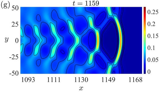
Figure 8 shows snapshots of the plan view of the water-surface displacement along with the corresponding bathymetry. In Figure 8a, we see the initial offshore water-surface displacement at . The smooth step then evolves into an undular bore in the offshore region as shown in Figure 8b. At time (Figure 8c), the undular bore encounters the toe of the continental slope and refracts about the crest of the ridge. In Figure 8d,e, the lead crest of the undular bore begins to straighten out while “radiating” waves emerge from the ends of the stem; this is similar to the pattern observed in the solitary wave case, as discussed in Section 3.1. At time (Figure 8f), it appears that the center of the waveform begins to bow forward which continues in Figure 8g,h. At time , (Figure 8i), the amplitude at the valley () becomes greater than at the ridge. In Figure 8j, solitons disintegrate from the front of the undular bore, resulting in a total of five solitary waves that have emerged at time as shown in Figure 8k.
Figure 9 shows the spatial evolution of the lead-wave amplitude of the 2D undular bore against location. The amplitude at the ridge () is represented by a solid line and the amplitude at the valley () is represented by a dashed line. The dotted line represents the amplitude of the lead crest of the undular bore for the 1D case which is discussed later in Section 3.2.1. The amplitude at is , which represents the height immediately after the intial water-surface displacement is set in motion. This initial height is in agreement with the prediction given by the method of characteristics for the nonlinear-nondispersive shallow-water-wave equation for a dam-break initial condition:
Soon after, the amplitude of the lead wave of the undular bore slowly increases until reaching . Once the undular bore encounters the sloping bed, we see that the amplitude at the ridge () quickly increases, reaching a maximum value of at , and the amplitude in the valley decreases, reaching a minimum value of at . The amplitude then behaves in a reciprocating fashion, creating a saw-tooth pattern. The amplitude at is roughly out of phase with the amplitude at . It appears though that the amplitude may approach an asymptotic state given a sufficient amount of time. For the 1D case that is represented by the dotted line in Figure 9, the amplitude increases monotonically until reaching the asymptotic value of after reaching the plateau. It appears that the amplitudes for the 1D and 2D cases become similar in the limit as . Recall that the amplitudes for the 1D and 2D cases of the solitary waves are different ( for the 1D case and for the 2D case) as .
The spatial phase lag is presented in Figure 10 for the 2D undular bore case. The phase lag remains at until encountering the toe of the bed slope at . At this point, a positive phase lag is created from the undular bore refracting about the crest of the continental shelf. A maximum value of is attained at . However, the spatial phase lag then sharply decreases to a minimum value of at . It appears that the phase lag is approaching an asymptotic value such that as . Note that, unlike the solitary wave case (Figure 5), the magnitudes of the maximum and minimum phase lags are similar for the undular bore.
3.2.1. Undular Bore Propagation over a Continental Shelf with no Lateral Variation
For comparison, we perform numerical experiments where an undular bore propagates over a smooth step into shallower waters without lateral variation (see the sketch in Figure 11). The same initial conditions along as (17) is applied. In this numerical experiment, we set , , , and .
Snapshots of the entire domain are presented in Figure 12. The initial conditions are shown in Figure 12a. The smooth step then evolves into an undular bore and a dispersive rarefaction wave with an expanding mean water depth, which separates the two ends of the waveform. The mean water depth is equivalent to the height predicted by Equation (18). Once encountering the toe of the continental slope, the undular bore shoals, and a careful observation in Figure 12c reveals the occurrence of energy reflection at time . Note that, at the beginning of the simulation, there are only two mean water depths. However, after the undular bore climbs up and passes over the sloping region, five distinct mean water depths can be identified at as shown in Figure 13. We may roughly partition these depths into the following regions: (1): for ; (2): for ; (3): for ; (4): for ; and (5): for . Regions (1), (2), and (5) are relatively straightforward to interpret. However, regions (3) and (4) require some explanations. Within region (4), the velocity field reaches an essentially steady flow condition. This is supported by Figure 14 which displays the depth-averaged horizontal velocity plotted against time at locations and . After about , the velocity appears to maintain the steady state. Note that the depth-averaged horizontal velocity is defined as
in which u is the horizontal fluid velocity and is the local total water depth. The fluid velocities are normalized by . The vertical component of the velocity is essentially nil. For an inviscid and homogeneous fluid, the total energy head (total mechanical energy plus pressure work per unit fluid weight) must be conserved. Therefore:
where and are the specific energy before and after the bed slope, respectively, which are defined as:
where the subscripts 3 and 4 refer to the values in the regions 3 and 4, respectively, (see Figure 13), and H is the total water depth. Following this notation, the height of the step can be given by the difference in the bed elevations: . From Equations (20) and (21), the theoretical total water depth at region 4 can be computed and found to be 0.556. This is calculated from the numerical data attained at with , , , and . The actual value attained from the numerical experiment was , resulting in no error up to the first three decimal places.
The analysis between regions (3) and (4) indicates that the flow is subcritical relative to the laboratory coordinate, and a standard analysis of the specific energy in the area of open-channel flows (see e.g., Henderson [26]) can be applicable here for the quasi-steady flow condition.
4. Discussion
Numerical experiments are performed for a solitary wave and an undular bore evolving over a continental shelf containing a lateral variability. The repetitious ridge-and-valley pattern of the continental shelf causes the incident wave to deform due to the effects of refraction, diffraction, and shoaling. The local wave focusing produces the formation of a stem-like wave pattern that results from the spatially merging wave. The stem-like formation at the merging location emanates “radiating” trailing oblique waves from the edges of the stem. These local interactions on the ridge are similar to the interaction of V-shaped solitary waves in a uniform depth [27], which also produce trailing wave radiation. These radiating waves are the source of additional wave-energy dispersion. Consequently, the energy of the solitary wave climbing over the 2D continental slope is less than the comparable 1D case (see Figure 4). On the other hand, the energy loss in the leading wave of the undular bore is substantially smaller than the case of the solitary wave (Figure 9). This is because the wave emanating from the stem interacts with the subsequent wave of the undular bore; the radiated wave cannot freely disperse behind the leading wave. The accumulation in energy of the obliquely radiating wave tends to maintain the leading-wave amplitude of the undular bore. The foregoing explanation can be supported by the comparison of our numerical results shown in Figure 2f for the solitary wave and Figure 8f for the undular bore.
After the solitary wave reaches the plateau, soliton fissioning occurs, which results in the formation of two distinct solitary waves in the simulation. The numerical results of the soliton fission for solitary waves propagating over both the 1D and 2D cases agree with the analytical prediction given by Equation (16). After a sufficient amount of time, the solitary wave recovers its characteristic form, approaching a steadily propagating state. It is found that the amplitude of the 1D propagation case approaches a greater asymptotic value than for the 2D propagation case. This difference in amplitude appears to be a result of extra energy dispersion caused by the formation of the obliquely radiating waves, which is allowed to occur in the 2D case.
Results were presented on an undular bore evolving from dam-break initial conditions and then propagating over a smooth depth transition from deep to shallow water. Note that this initial condition resembles an ideal model of a co-seismic tsunami source. After the wave reaches the plateau region, multiple (in this case five) discrete solitary waves appear to disintegrate from the leading portion of the undular bore. This particular result has potential applications in engineering. For instance, after a tsunami propagates over a continental slope, our results demonstrate the possibility for multiple localized waves of significant amplitude to advance over a broad continental shelf and ultimately inundate the shore with a series of waves.
The present results demonstrate the uncertainty in predicting the critical locations of the greatest tsunami amplitude. From linear theory, we anticipate that the greatest amplitude should be observed along the ridge (). However, our numerical experiments reveal that there is a laterally reciprocating variability in the amplification which occurs as a consequence of the nonlinear dependence of the phase speed on the amplitude.
The mean water surface of the entire domain was also examined for an undular bore propagating over the 1D continental shelf. Initially, we see that the water surface only contains two mean depths, but after the undular bore propagates well beyond the continental shelf, we find a total of five mean water depths over different segments of the domain. It appears that specific energy (a standard parameter used to analyze 1D steady open-channel flows) can be used to accurately predict the height of these mean water depths before and after the continental shelf.
5. Conclusions
Many previous studies on tsunami propagation over a continental slope assessed the problem for a 1D shelf configuration: i.e., no lateral variation. Here we examined long-wave (tsunami) transformations over a continental slope with a periodic lateral variation, considering two incident wave models: a solitary wave and an undular bore. The lateral variation causes the incident wave to refract, diffract and shoal along the trajectory of wave propagation. When the wave initially encounters the continental slope, shoaling occurs, placing the location of maximum amplitude over the ridge. Soon after, the location of maximum amplitude shifts to the valley due to the effects of wave nonlinearity and phase velocity in the 2D field. This transfer of energy then periodically shifts back and forth between the ridge and the valley. This process induces extra wave energy dispersion, and affects the energy distribution on the continental shelf after the incident wave climbs up the slope. Our findings demonstrate the importance in consideration of lateral variability of the continental slope for the evaluation of long-wave behaviors and consequences when it climbs up the continental slope.
The behaviors of localized long waves interacting and shoaling over a 2D bathymetry are primarily discussed in the context of length scales on the order of a continental shelf, where the corresponding waveform is a tsunami. None the less, the findings should be applicable to smaller scale nearshore waves interacting with the bathymetry as well.
Author Contributions
J.K. and H.Y. Contributed equally. All authors have read and agreed to the published version of the manuscript.
Funding
This research was partially funded by the US National Science Foundation grant number OCE-1830024.
Acknowledgments
J.K. was partially supported by Matt Evans.
Conflicts of Interest
The authors declare no conflict of interest.
References
- Synolakis, C.E. Green’s law and the evolution of solitary waves. Phys. Fluids 1991, 3, 490–491. [Google Scholar] [CrossRef]
- Synolakis, C.E.; Skjelbreia, J.E. Evolution of maximum amplitude of solitary waves on plane beaches. J. Waterw. Port Coast. Ocean Eng. 1993, 119, 323–342. [Google Scholar] [CrossRef]
- Miles, J. Solitary wave evolution over a gradual slope with turbulent friction. J. Phys. Oceanogr. 1983, 13, 551–553. [Google Scholar] [CrossRef] [Green Version]
- Grilli, S.T.; Subramanya, R.; Svendsen, I.A.; Veeramony, J. Shoaling of solitary waves on plane beaches. Oceanogr. Lit. Rev. 1995, 8, 608. [Google Scholar] [CrossRef] [Green Version]
- Guyenne, P.; Nicholls, D.P. Numerical simulation of solitary waves on plane slopes. Math. Comput. Simul. 2005, 69, 269–281. [Google Scholar] [CrossRef] [Green Version]
- Knowles, J.; Yeh, H. On shoaling of solitary waves. J. Fluid Mech. 2018, 30, 1073–1097. [Google Scholar] [CrossRef]
- Chen, Q.; Kirby, J.; Dalrymple, R.; Kennedy, A.; Chawla, A. Boussinesq modeling of wave transformation, breaking, and runup. II: 2D. J. Waterw. Port Coast. Ocean Eng. 2000, 126, 48–56. [Google Scholar] [CrossRef]
- Wei, G.; Kirby, J.T.; Grillis, S.T.; Subramanya, R. A fully nonlinear Boussinesq model for surface waves. Part I: Highly nonlinear unsteady waves. J. Fluid Mech. 1995, 294, 71–92. [Google Scholar] [CrossRef]
- Lynett, P.; Swigler, D.; Son, S.; Bryant, D.; Socolofsky, S. Experimental study of solitary wave evolution over a 3D shallow shelf. Int. Conf. Coastal. Eng. 2010, 1. [Google Scholar] [CrossRef] [Green Version]
- Lynett, P.; Swigler, D.; Safty, H.E.; Montoya, L.; Keen, A.S.; Son, S.; Higuera, P. Three-dimensional hydrodynamics associated with a solitary wave traveling over an alongshore variable shallow shelf. J. Waterw. Port Coast. Ocean Eng. 2019, 145, 04019024. [Google Scholar] [CrossRef]
- Liu, P.; Cho, L.-F.Y.; Briggs, M.J.; Kanoglu, U.; Synolakis, C.E. Runup of solitary waves on a circular island. J. Fluid Mech. 1995, 302, 259–285. [Google Scholar] [CrossRef]
- Yoshiki, Y.; Cheung, K.F.; Kowalik, Z. Depth-integrated, non-hydrostatic model with grid nesting for tsunami generation, propagation, and run-up. Int. J. Numer. Meth. Fluids 2010. [Google Scholar] [CrossRef]
- Shimozono, T. Long wave propagation and run-up in converging bays. J. Fluid Mech. 2016, 798, 457–484. [Google Scholar] [CrossRef]
- Favre, H. Etude Theorique et Experimental des Ondes de Translation dans les Canaux Decouverts; Dunad: Paris, France, 1935; p. 150. [Google Scholar]
- Peregrine, D.H. Calculations of the development of an undular bore. J. Phys. Oceanogr. 1966, 25, 321–330. [Google Scholar] [CrossRef]
- Sandover, J.A.; Taylor, C. Cnoidal waves and bores. La Houille Blance 1962, 3, 443–465. [Google Scholar] [CrossRef] [Green Version]
- Craig, W.; Sulem, C. Numerical simulation of gravity waves. J. Comput. Phys. 1993, 108, 73–83. [Google Scholar] [CrossRef]
- Zakharov, V.E. Stability of periodic waves of finite amplitude on the surface of a deep fluid. J. Appl. Mech. Tech. Phys. 1968, 9, 190–194. [Google Scholar] [CrossRef]
- Boyce, W.E.; DiPrima, R.C.; Meade, D.B. Elementary Differnetial Equations and Boundary Value Problems, Loose-Leaf Print Companion; John Wiley & Sons: Hoboken, NJ, USA, 2017. [Google Scholar]
- Dommermuth, D.G.; Yue, K.P. A high-order spectral method for the study of nonlinear gravity waves. J. Fluid Mech. 1987, 184, 267–288. [Google Scholar] [CrossRef]
- Gouin, M.; Ducrozet, G.; Ferrant, P. 2d and 3d nonlinear wave propagation over a non-uniform bottom by pseudo-spectral mehtod. In Proceedings of the 11th European Wave and Tidal Energy Conference (EWTEC), Nantes, France, 6–11 September 2015; Volume 8, p. 608. [Google Scholar]
- Grimshaw, R. The solitary wave in water of variable depth. Part 2. JFM 1971, 46, 611–622. [Google Scholar] [CrossRef]
- Yeh, H.; Li, W. Laboratory realization of KP-solitons. J. Phys. Conf. Ser. 2014, 482, 012046. [Google Scholar] [CrossRef] [Green Version]
- Kodama, Y.; Yeh, H. The kp theory and mach reflection. J. Fluid Mech. 2016, 800, 766–786. [Google Scholar] [CrossRef]
- Johnson, R.S. A Modern Introduction to the Mathematical Theory of Water Waves; Cambridge University Press: Cambridge, UK, 1997; p. 276. [Google Scholar]
- Henderson, F.M. Open Channel Flow; MacMillan: New York, NY, USA, 1966. [Google Scholar]
- Kodama, Y.; Oikawa, M.; Tsuji, H. Soliton solutions of the kp equation with v-shape initial waves. J. Phys. A Math. Theor. 2009, 42, 312001. [Google Scholar] [CrossRef] [Green Version]
Figure 1.
Plan view of the bathymetry with periodic lateral variation.

Figure 2.
Contour plots of the water-surface displacement for the solitary wave propagating over 2D bathymetry at times: (a) , (b) , (c) , (d) , (e) , (f) , (g) , (h) , (i) , (j) , and (k) . (l) Bathymetry (note the different and scales).
Figure 2.
Contour plots of the water-surface displacement for the solitary wave propagating over 2D bathymetry at times: (a) , (b) , (c) , (d) , (e) , (f) , (g) , (h) , (i) , (j) , and (k) . (l) Bathymetry (note the different and scales).

Figure 3.
Water-surface displacement of solitary wave for for the 2D bathymetry (12) at time along center transect (). (a) Water-surface displacement on the plateau of the bathymetry. Overlay of the higher-order solitary-wave solution (dashed line) with the numerical solution (solid line): (b) lead solitary wave, (c) intermediate wave, and (d) trailing wave.

Figure 4.
Amplitude variation of the solitary wave along the ridge (solid line) and along the valley (dashed line) over the 2D bathymetry (12). The dotted line represents the amplitude of the solitary wave for the 1D wave-propagation case.
Figure 4.
Amplitude variation of the solitary wave along the ridge (solid line) and along the valley (dashed line) over the 2D bathymetry (12). The dotted line represents the amplitude of the solitary wave for the 1D wave-propagation case.

Figure 5.
Spatial phase lag between locations at and for the solitary wave over the 2D bathymetry (12). Note that , where gives the coordinate of the lead crest of the solitary wave at , and gives the coordinate of the leading crest at .
Figure 5.
Spatial phase lag between locations at and for the solitary wave over the 2D bathymetry (12). Note that , where gives the coordinate of the lead crest of the solitary wave at , and gives the coordinate of the leading crest at .

Figure 6.
Evolution of solitary wave over the 1D bathymetry (15) for times (a) , (b) , (c) , and (d) .
Figure 6.
Evolution of solitary wave over the 1D bathymetry (15) for times (a) , (b) , (c) , and (d) .

Figure 7.
Water-surface displacement of solitary wave with on the plateau fo the 1D bathymetry (15) at time along center transect (). (a) Water-surface displacement on the plateau of the bathymetry. Overlay of the higher-order solitary-wave solution (dashed line) with the numerical solution (solid line): (b) Lead solitary wave, (c) intermediate wave, and (d) trailing wave.

Figure 8.
Contour plots of the water-surface displacement for the undular bore propagating over 2D bathymetry at times: (a) , (b) , (c) , (d) , (e) , (f) , (g) , (h) , (i) , (j) , (k) . (l) Bathymetry (note the different and scales).
Figure 8.
Contour plots of the water-surface displacement for the undular bore propagating over 2D bathymetry at times: (a) , (b) , (c) , (d) , (e) , (f) , (g) , (h) , (i) , (j) , (k) . (l) Bathymetry (note the different and scales).

Figure 9.
Amplitude variation of undular bore along the ridge (solid line) and along the valley (dashed line) over the 2D bathymetry (12). The dotted line represents the amplitude of the undular bore for the 1D wave-propagation case.
Figure 9.
Amplitude variation of undular bore along the ridge (solid line) and along the valley (dashed line) over the 2D bathymetry (12). The dotted line represents the amplitude of the undular bore for the 1D wave-propagation case.

Figure 10.
Spatial phase lag between locations at and for undular bore over the 2D bathymetry (12). Note that , where gives the coordinate of the lead crest of the undular bore at , and gives the coordinate of the leading crest at .
Figure 10.
Spatial phase lag between locations at and for undular bore over the 2D bathymetry (12). Note that , where gives the coordinate of the lead crest of the undular bore at , and gives the coordinate of the leading crest at .

Figure 11.
Definition sketch of the initial dam-break conditions for undular bore.

Figure 12.
Water-surface displacement of undular bore propagating over the 1D continental slope at times: (a) , (b) , (c) , and (d) .
Figure 12.
Water-surface displacement of undular bore propagating over the 1D continental slope at times: (a) , (b) , (c) , and (d) .

Figure 13.
Water-surface displacement of undular bore propagating over the 1D continental shelf, displaying five different mean water depths at time .
Figure 13.
Water-surface displacement of undular bore propagating over the 1D continental shelf, displaying five different mean water depths at time .

Figure 14.
Temporal variation of depth-averaged horizontal velocity for undular bore over the 1D bathymetry at the locations (a) and (b) . At , the leading two waves are solitary waves. The horizontal velocity approaches a steady state after approximately .
Figure 14.
Temporal variation of depth-averaged horizontal velocity for undular bore over the 1D bathymetry at the locations (a) and (b) . At , the leading two waves are solitary waves. The horizontal velocity approaches a steady state after approximately .

© 2020 by the authors. Licensee MDPI, Basel, Switzerland. This article is an open access article distributed under the terms and conditions of the Creative Commons Attribution (CC BY) license (http://creativecommons.org/licenses/by/4.0/).
Share and Cite
MDPI and ACS Style
Knowles, J.; Yeh, H. Long-Wave Penetration through a Laterally Periodic Continental Shelf. J. Mar. Sci. Eng. 2020, 8, 241. https://0-doi-org.brum.beds.ac.uk/10.3390/jmse8040241
AMA Style
Knowles J, Yeh H. Long-Wave Penetration through a Laterally Periodic Continental Shelf. Journal of Marine Science and Engineering. 2020; 8(4):241. https://0-doi-org.brum.beds.ac.uk/10.3390/jmse8040241
Chicago/Turabian StyleKnowles, Jeffrey, and Harry Yeh. 2020. "Long-Wave Penetration through a Laterally Periodic Continental Shelf" Journal of Marine Science and Engineering 8, no. 4: 241. https://0-doi-org.brum.beds.ac.uk/10.3390/jmse8040241
Note that from the first issue of 2016, this journal uses article numbers instead of page numbers. See further details here.