Denoising Effect of Jason-1 Altimeter Waveforms with Singular Spectrum Analysis: A Case Study of Modelling Mean Sea Surface Height over South China Sea

Abstract

Altimeter waveforms are usually contaminated due to nonmarine surfaces or inhomogeneous sea state conditions. The present work aimed to present how the singular spectrum analysis (SSA) can be used to reduce the noise level in Jason-1 altimeter waveforms to obtain SSA-denoised waveforms, improving the accuracy of a mean sea surface height (MSSH) model. Comparing the retracked sea surface heights (SSHs) by a 50% threshold retracker for the SSA-denoised waveforms with those for the raw waveforms, the results indicated that SSA allowed a noise reduction on Jason-1 waveforms, improving the accuracy of retracked SSHs. The MSSH model (called Model 1) over the South China Sea with a grid of 2′ × 2′ was established from the retracked SSHs of Jason-1 by the 50% threshold retracker for the SSA-denoised waveforms. Comparing Model 1 and Model 2 (established from the retracked SSHs by the 50% threshold retracker for the raw waveforms) with the CLS15 and DTU18 models in the South China Sea, it was found that the accuracy of Model 1 was higher than that of Model 2, which indicates that using SSA to reduce noise level in Jason-1 waveforms can effectively improve the accuracy of the MSSH model.

1. Introduction

Satellite radar altimeters provide information on the Earth’s surface by transmitting a series of radio-frequency pulses and recording their echo waveforms [1]. Satellite altimetry has been widely used in geodesy, geophysics, and oceanography [2]. Some satellite altimetry products have been obtained using satellite altimeter data, e.g., ocean tide models, gravity field models, and mean sea surface height (MSSH) models. Among them, the MSSH model is the time-averaged physical height of the ocean’s surface [3] and is an essential and important parameter to support oceanographic and geophysical studies [4]. The accuracy of the MSSH model is affected by the quality of satellite altimeter data, as well as the theory and methods of data processing. With the improvement of satellite altimetry error correction theory and data processing methods [5], using waveform retracking to improve the quality of altimeter data has gradually become the key to improving the accuracy and application of altimeter data, especially in coastal regions [6].

Altimeter waveforms are usually contaminated due to land, island, sea reef, sea ice, seabed terrain, etc. If the extracted ranges from these corrupted waveforms are used, sea levels calculated from these ranges will be incorrect as well. Waveform retracking is a method to find the right tracking gate, cutting the midpoint of the leading edge from these corrupted waveforms to extract the actual ranges [7]. So far, the waveform retracking technique has developed a variety of retracking methods, which are mainly divided into two categories: One based on the empirical statistical properties of the waveform data, and the other based on fitting functional model [2,8]. These retracking methods can improve the quality of altimeter data, but the accuracy of the data still cannot meet the actual needs [9,10,11]. Besides, the noise information contained in altimeter waveforms is not considered during the process of waveform retracking.

Several altimeter waveforms are connected end-to-end to form a waveform series, which oscillates periodically with the number of the waveform samples (e.g., the waveform samples of Jason-1 are 104). The altimeter waveform can be regarded as composed of two parts: The main waveform information and the noise information. The main waveform information includes the thermal noise area, leading edge, and trailing edge of the altimeter waveform, while the noise information is caused by reflective surfaces such as land, sea, glaciers, etc. By performing singular spectrum analysis (SSA) on the waveform series, the noise information contained in altimeter waveforms can be reduced, so that useful waveform information is extracted.

SSA is a nonparametric method of time series analysis [12,13]. It can reduce noise information from time series containing noise and extract as much reliable information as possible [14,15]. This method has been widely used in meteorology, climatology, geophysics, and other fields [13]. Therefore, SSA can be used to decompose and reconstruct the waveform series, reduce the noise level in altimeter waveforms, and obtain SSA-denoised waveforms. Then, these SSA-denoised waveforms are reprocessed by the waveform retracking technique to improve the accuracy and application of altimeter data.

The goal of this work was to reduce the noise level in Jason-1 altimeter waveforms with SSA to improve the accuracy of Jason-1 altimeter data, and to validate whether SSA can effectively improve the accuracy of MSSH model over the South China Sea established from SSA-denoised waveforms retracking of Jason-1 data. The structure of the thesis is as follows: Section 2 mainly introduces the study area, the data used, and data processing methods; Section 3 involves the results; Section 4 presents MSSH model over the South China Sea established from SSA-denoised waveforms retracking of Jason-1 data and validates whether SSA can effectively improve the accuracy of MSSH model; and the main conclusions and perspectives are given in Section 5.

2. Study Area, Data, and Data Processing Methods

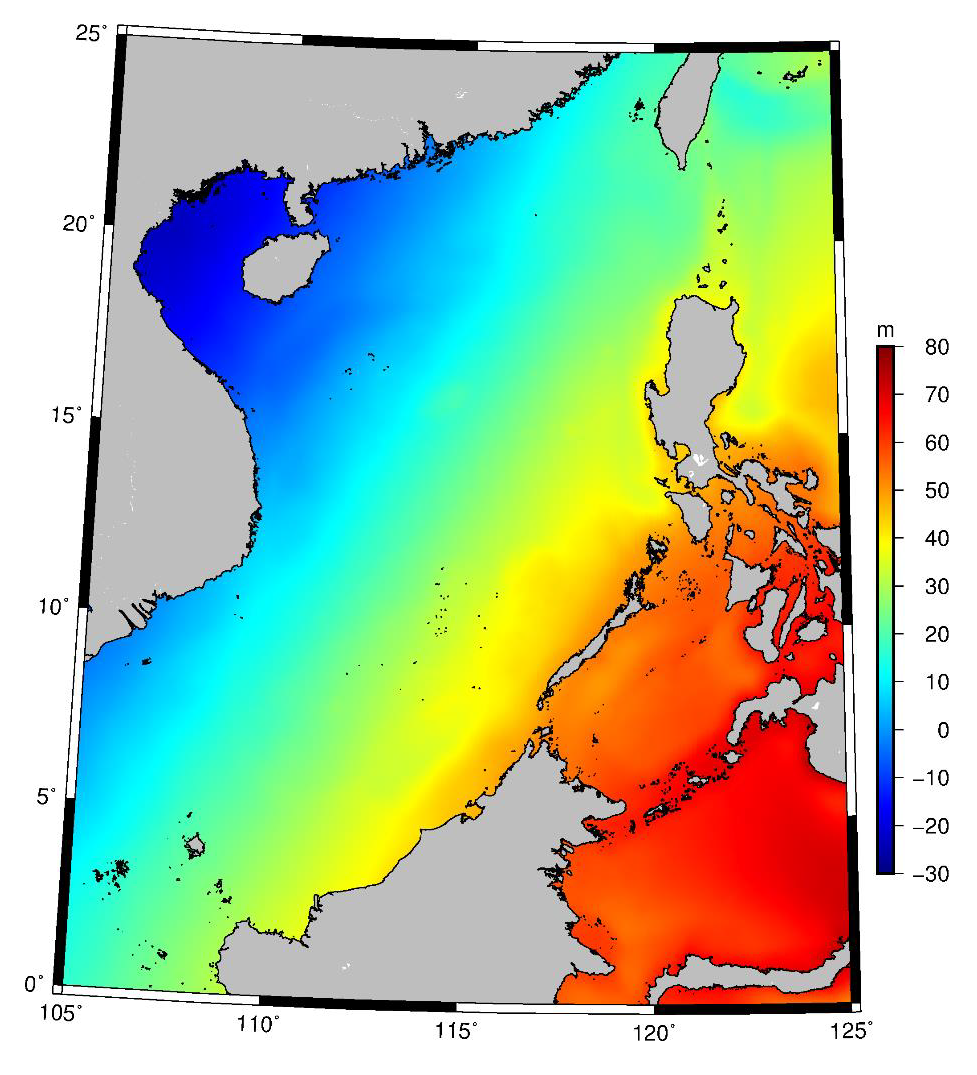
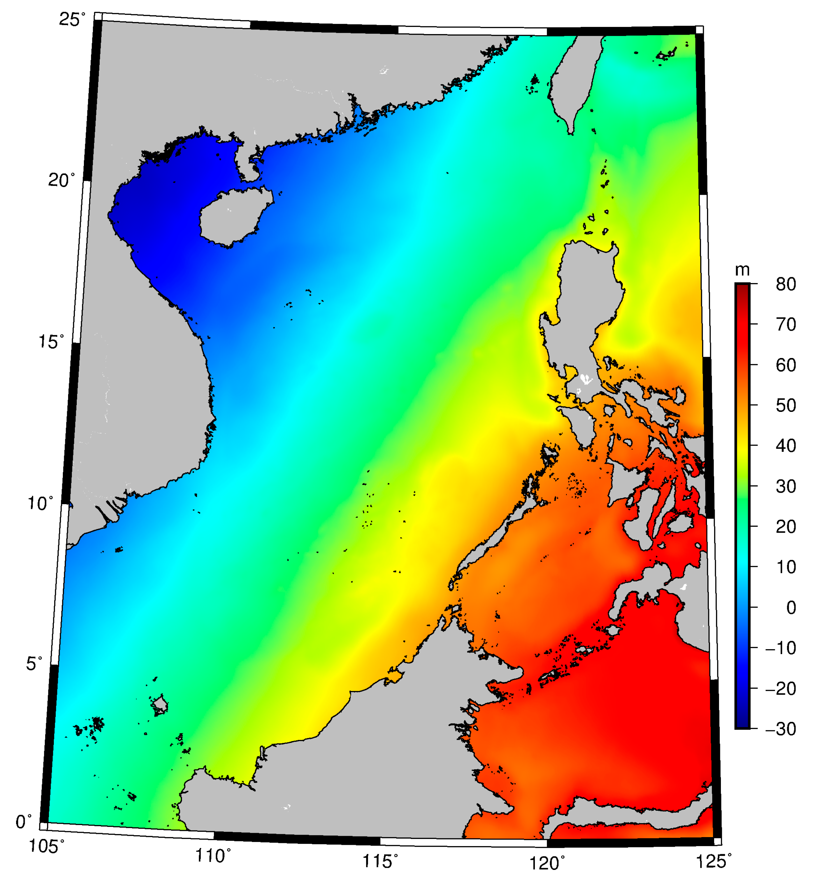
2.1. Study Area and Data

The area around the South China Sea, covering 0°–25° N, 105°–125° E, was selected as the study area. The South China Sea belongs to the western Pacific Ocean and is one of the three marginal seas in Asia. It is located at the intersection of the Eurasian plate, Indo-Australian plate, and Pacific plate. Covering an area of about 3.5 million square kilometers, it is the third largest sea in the world, following the Coral Sea in the South Pacific and the Arabian Sea of the Indian Ocean. With an average depth of 1212 m and the deepest point of 5377 m, the South China Sea is virtually surrounded by land, peninsulas, and islands. The South China Sea is linked in the northeast to the East China Sea and the Pacific Ocean through the Taiwan Strait; in the south to the Java Sea, the Andaman Sea, and the Indian Ocean through the Malacca Strait; and in the east to the Sulu Sea through the Bashi Strait. Located in the low-latitude region, the South China Sea has the warmest climate of all tropical deep seas of China, with a high surface water temperature (25 °C–28 °C), small annual temperature variation (3 °C–4 °C), year-round high temperature and humidity, and long summer without winter. It has a maximal salinity of 35‰ and tidal difference below 2 m.

Jason-1 was launched on 7 December 2001 and decommissioned on 1 July 2013, obtaining about 11.5 years of altimeter waveforms data [16]. These data were used in our study as listed in

Table 1. Altimeter waveforms data of Jason-1 missions.

Missions	Data Duration	Cycle Number	Orbit Altitude (km)	Mean Track Separation at the Equator (km)
ERM1	2002/01/15–2009/01/26	001-259	1336	315
ERM2	2009/02/10–2012/03/03	262-374	1336	315
GM	2012/05/07–2013/06/21	500-537	1324	7

. The data, spanning from 2002 to 2013, are version E of sensor geophysical data records (SGDR) products (including the so-called measured 20-Hz waveforms) provided by Archiving, Validation, and Interpretation of Satellite Oceanographic Data (AVISO). The orbit of Jason-1 had three different phrases. From its launch, its orbit had the same ground tracks as TOPEX/Poseidon (T/P), which was the first phrase. In mid-February, 2009 (cycle 262), Jason-1 assumed a new orbit midway between its original ground tracks, which was the second phrase. At the end of February and in early March 2012, it began a series of maneuvers to reduce the orbit on a geodetic orbit, which was the third phrase. In the former two phrases, Jason-1 performed exactly repeated mission (ERM) (the mission of the first phrase hereafter called ERM1 and the second phrase ERM2) with a cycle of 9.9 days. In the third phrase, Jason-1 performed the geodetic mission (GM), and its orbit was a drifting orbit with a cycle of 406 days and some sub-cycles of 3.9–10.9–47.5–179.5 days.

Figure 1 is the ground tracks map of Jason-1 in South China Sea. Figure 1a is the ground tracks map of ERM1 and ERM2, and Figure 1b is that of GM.

2.2. Data Processing Methods

Jason-1 waveforms were connected end-to-end to form the waveform series (one pass corresponded to one waveform series), and the waveform series was denoised with SSA to obtain the SSA-denoised waveforms. Then, these SSA-denoised waveforms were retracked by a 50% threshold retracker to obtain the retracked sea surface heights (SSHs). The process of Jason-1 waveforms processing is shown in Figure 2.

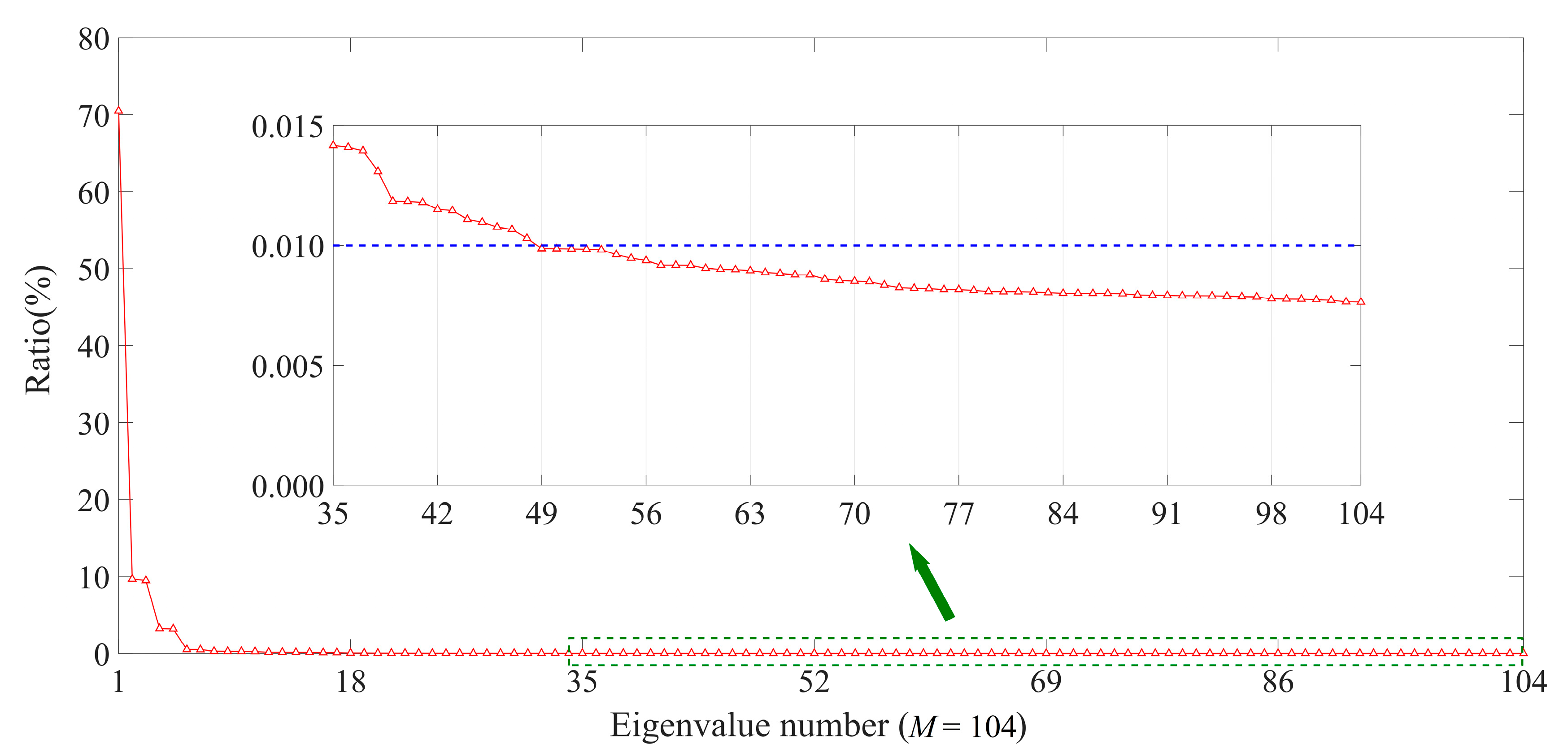
2.2.1. Singular Spectrum Analysis (SSA) Applied to Altimeter Waveforms

SSA constructs a multidimensional trajectory matrix for a waveform series and decomposes and reconstructs the trajectory matrix to extract signals that represent the main waveform information and noise information.

Assume that a waveform series consisting of i waveforms is $X(t)\{x_t:1<t<N\},N=i\times 104$ (104 is the number of waveform samples of Jason-1). SSA was used to denoise this waveform series, and the process was mainly divided into four steps [14,15]:

(1) Embedding

Because the oscillation period of the waveform series is 104, the SSA method with a window of 104 was adapted to reduce the noise information of the waveform series. Defining the delay vector $X_k$ as $X_k={\{x_k,\cdots ,x_{k+M-1}\}}^T,1\le k\le N-M+1$, the trajectory matrix S of the waveform series can be expressed as:

$$S=[\begin{array}{cccc}{X}_1& X_2& \cdots & X_{N-M+1}\end{array}]=\left[\begin{array}{ccc}{x}_1& \cdots & x_{N-M+1}\\ ⋮& \ddots & ⋮\\ x_M& \cdots & x_N\end{array}\right]$$

(1)

where N is the waveform series length and M is the window ($M=104$).

(2) Singular Value Decomposition (SVD)

SVD was performed on the covariance matrix $R=S{S}^T$ of the trajectory matrix S to obtain M eigenvalues in descending order ${\lambda }_1\ge {\lambda }_2\ge \cdots \ge {\lambda }_M$ and corresponding eigenvectors $U_1,U_2,\cdots ,U_M$. Then, the principal components (PC) $V_i$ can be expressed as $V_i=S^T{U}_i/\sqrt{{\lambda }_i},i=\{1,\cdots ,M\}$, and the trajectory matrix S can be expressed as the sum of the elementary matrices $S_i$ ($S_i=\sqrt{{\lambda }_i}{U}_i{V}_i^T,i=\{1,\cdots ,M\}$) obtained by SVD, i.e.,

$$S=S_1+S_2+\cdots +S_M$$

(2)

(3) Grouping

The waveform series can be seen as being composed of two parts: The main waveform information and the noise information. Therefore, the subscript $D=\{1,\cdots ,M\}$ of the elementary matrix $S_i$ was divided into two disjoint subsets, namely $D_1=\{1,\cdots ,l\},1<l<M$ containing the first few leading components that describe the main waveform information, and $D_2=D-D_1$ containing the residual components that describe the noise information. Then, the trajectory matrix S can be decomposed into two parts, $S^{D_1}=S_1+S_2+\cdots +S_l$ and $S^{D_2}=S_{l+1}+S_{l+2}+\cdots +S_M$, namely:

$$S=S^{D_1}+S^{D_2}$$

(3)

The parameter l denotes the leading components, which provides a good description of the main waveform information, and the lower M-l components represent the noise information. If l is too small, a part of the main waveform information will miss. Alternatively, if l is too large, a part of the main waveform information is approximated with the noise information. Currently, there is no clear standard for determining this parameter [13]. To properly choose the parameter l, the ratio calculated in Equation (4) was used to estimate the contribution of the i-th candidate principal component corresponding to the raw waveform series.

$${\mathrm{Ratio}}_i={\lambda }_i/{\displaystyle \sum _{i=1}^M{\lambda }_i}$$

(4)

where λ_i is the i-th eigenvalue.

(4) Reconstruction

Reconstruction was performed to restore $S^{D_1}$ and $S^{D_2}$ in Equation (3) to new series $X^{D_1}(t)$ and $X^{D_2}(t)$ of length N, respectively. Taking reconstruction $S^{D_1}$ as an exa $M^{*}=\min (M,N-M+1)$ mple to describe its specific process and assuming that the element in $S^{D_1}$ is $y_{i,j}$, and $K^{*}=\max (M,N-M+1)$, the reconstruction of $S^{D_1}$ into the new series $X^{D_1}(t)\{g_t:1<t<N\}$ can be obtained as follows:

$$g_t=\{\begin{array}{ll}\frac{1}{t}{\displaystyle \sum _{i=1}^t{y}_{i,t-i+1}},\hfill & 1\le t<M^{*}\\ \frac{1}{M^{*}}{\displaystyle \sum _{i=1}^{M^{*}}{y}_{i,t-i+1}},\hfill & M^{*}\le t\le K^{*}\\ \frac{1}{N-t+1}{\displaystyle \sum _{i=t-K^{*}+1}^{N-K^{*}+1}{y}_{i,t-i+1}},\hfill & K^{*}<t\le N\end{array}$$

(5)

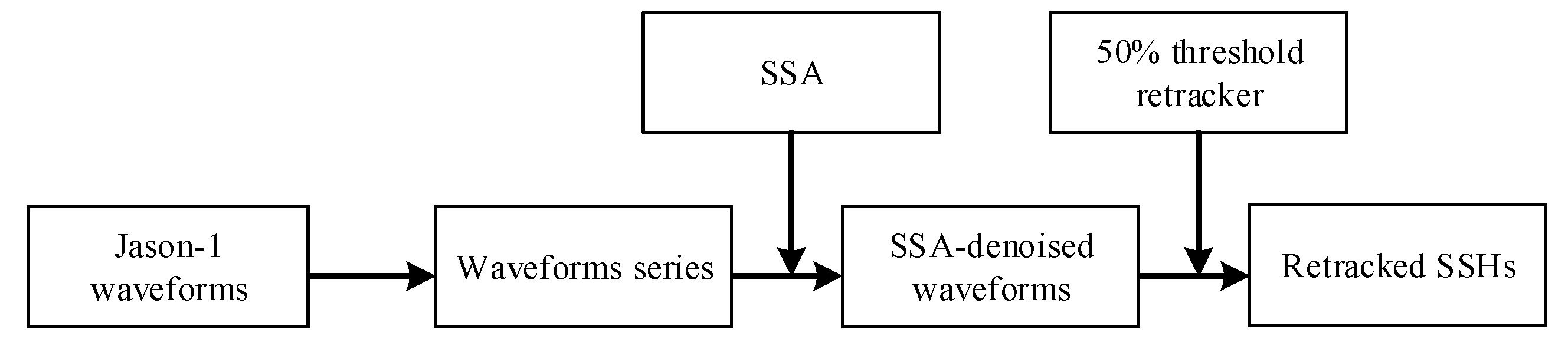
2.2.2. Waveform Retracking Method

Accurate range estimates were obtained using methods of waveform retracking (e.g., Ocean, Ice-2, Belta5, Threshold) [17]. These retracking methods and their applications to the coastal altimeter waveform have been reviewed in Gommenginger et al. [8]. Some studies have shown that the standard Ocean retracking method, Ice-2 retracking algorithm, and Belta5 retracker are not appropriate for complex coastal waveforms [6,8,10,17]. However, the threshold retracker is easy to implement and successful in producing valid SSHs from coastal altimeter waveform retracking [6,17,18,19,20]. Therefore, the threshold retracker was used in our study.

The threshold retracker was developed by Davis [21,22]. It is based upon the dimensions of the rectangle computed using the offset center of gravity (OCOG) retracking algorithm [6,8]. The threshold level is referenced to the OCOG amplitude as 25%, 50%, and 75% of the amplitude. The retracking gate estimate is determined by linearly interpolating between adjacent samples of a threshold crossing the steep part of the leading-edge slope of the waveform [8]. The selection of the appropriate threshold level (such as 25%, 50%, or 75% of the OCOG amplitude) is very important. However, a reasonable choice is very difficult and difficult to grasp [6,19]. For the coastal altimeter waveform, a 50% threshold level retracking can usually obtain better results [19]. The formula and explanations in the calculation of the 50% threshold retracker have been presented by Deng [6] and Gommenginger et al. [8].

2.2.3. Estimating Sea Surface Height

The retracked gate was estimated from 50% threshold retracker to determine retracked range correction by [5]:

$$\Delta R_{\mathrm{Ret}}=\frac{c}{2}\times \tau \times \left(G_{\mathrm{Ret}}-G_{\mathrm{Re}\mathrm{f}}\right)$$

(6)

where $\Delta R_{\mathrm{Ret}}$ is the range correction derived from the waveform retracking methods (m), c is the light velocity in vacuum, τ is the time interval for one gate Jason-1 satellite (3.125 ns), G_Ret is the retracked gate estimated from the 50% threshold retracker, and G_Ref is the reference tracking gate on-board observation of Jason-1 satellite (32, in unit of gates) [23]. Then, the precise SSH value of retracking waveform was calculated by Equation (7) [5,16]:

$$SS{H}_{\mathrm{corr}}=R_{\mathrm{Alt}}-(R+\Delta R_{\mathrm{ret}})-corr$$

(7)

where SSH_corr is the retracked SSH (m); R_Alt is the satellite altitude (m); R is the range of satellite measurement (m); and corr is the error correction (m), which includes wet troposphere correction, dry troposphere correction, ionosphere correction, sea-state correction, dynamic atmospheric correction, ocean tide correction, solid Earth-tide correction, loading tide correction, and pole tide correction. All these error corrections can be found in Jason-1 SGDR products.

3. Results

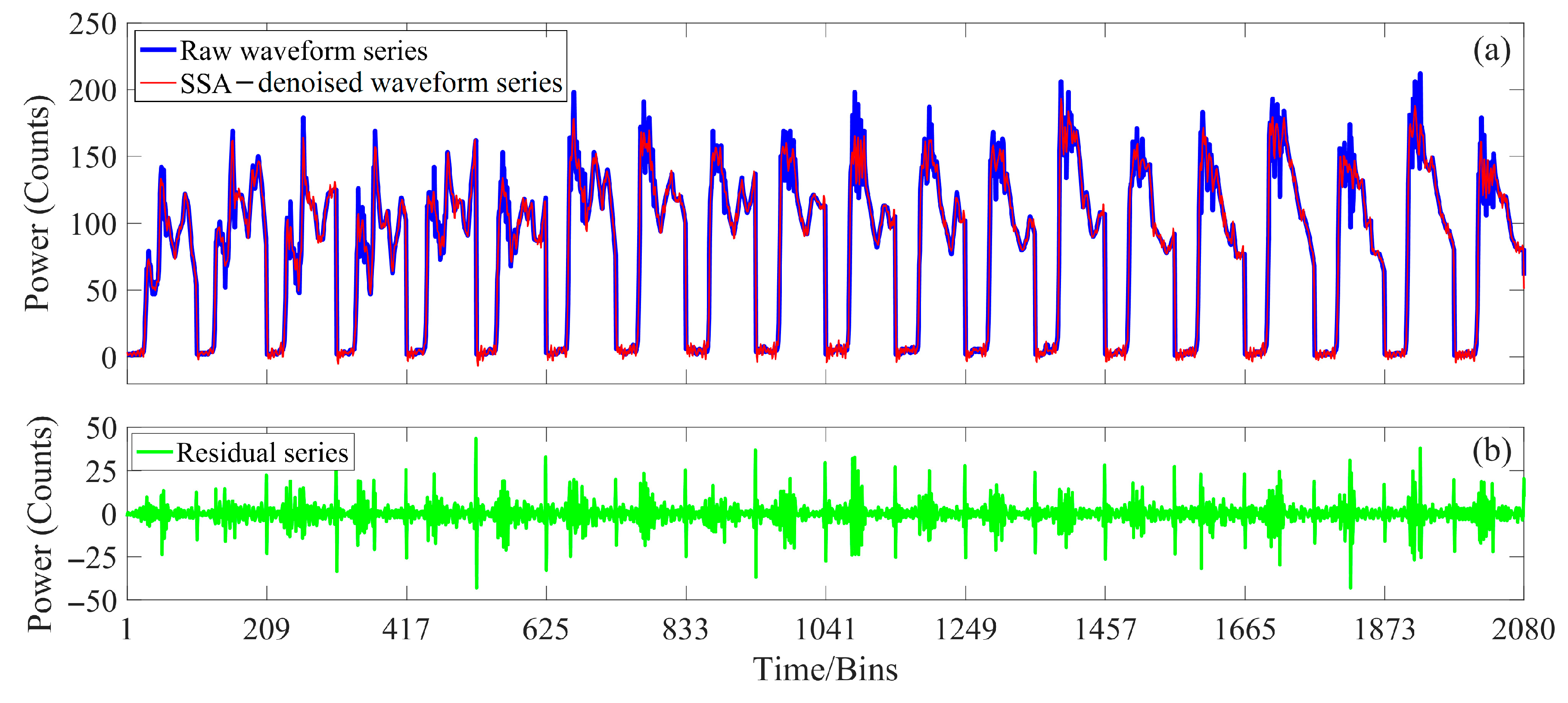
3.1. SSA-Denoised Waveform Series

We experimented with the 20-Hz waveforms data of Jason-1 cycle 340 pass 153 from 13.80° N to 21.75° N (pass with purple color in Figure 1, hereafter called c340-p153 track). This track had a total of 3118 waveforms and contained the altimeter data moving from both land to ocean and ocean to land. The deepest part of the waters that this track moved was about 1730 m, and the shallowest part was about 7 m. The c340-p153 track had sufficient data volume and a certain representativeness. The waveforms of the c340-p153 track were connected end-to-end to construct a waveform series with length of $N=3118\times 104$. Then, this waveform series was denoised with SSA.

The main purpose of the waveform retracker is to find the position of the leading-edge component with respect to the fixed nominal tracking point [6,8]. Therefore, it is critical to retain the slope information of the leading-edge component when performing noise reduction of the waveform series with SSA. It was assumed that a component with a ratio lower than 0.01% was considered as the noise information. That is, the ratio of 0.01% was used as a boundary value to distinguish the main waveform information and the noise information. The components with a ratio higher than 0.01% were classified as the main waveform information, and those lower than 0.01% were classified as the noise information. This means we can reconstruct the main waveform information from the components with a ratio higher than 0.01%.

Figure 3 presents the contribution ratio of the eigenvalues ${\left\{{\lambda }_i\right\}}_i^M$ corresponding to the raw waveform series. As can be seen from Figure 3, except for the ratio of the first eigenvalue reaching about 70.5%, the others were less than 10%, and the ratio of each eigenvalue starting from the 49th eigenvalue was within 0.01%. The ratio of the first 48 eigenvalues was more than 99%. Therefore, it was preferable to choose l = 48 in reconstruction to obtain the SSA-denoised waveform series. Thus, the main waveform information can be well preserved.

Figure 4a is the beginning part of the raw waveform series and the SSA-denoised waveform series, the latter corresponding to the main waveform information. Figure 4b is the beginning part of the residual series (i.e., noise information of the waveform series), defined as the difference between the raw and SSA-denoised waveform series. As can be seen from Figure 4, by comparison, the raw waveforms and the SSA-denoised waveforms mainly differed in the thermal noise component and amplitude, while the slope information of leading-edge component was well retained. This indicates that SSA allowed a noise reduction on Jason-1 waveforms. The larger amplitude of the residual series in Figure 4b was mainly concentrated on the junction of different waveforms. The reason is that the trailing edge component of the waveform was affected by the low-frequency signal of the thermal noise component of the following waveform. However, the leading edge was less affected.

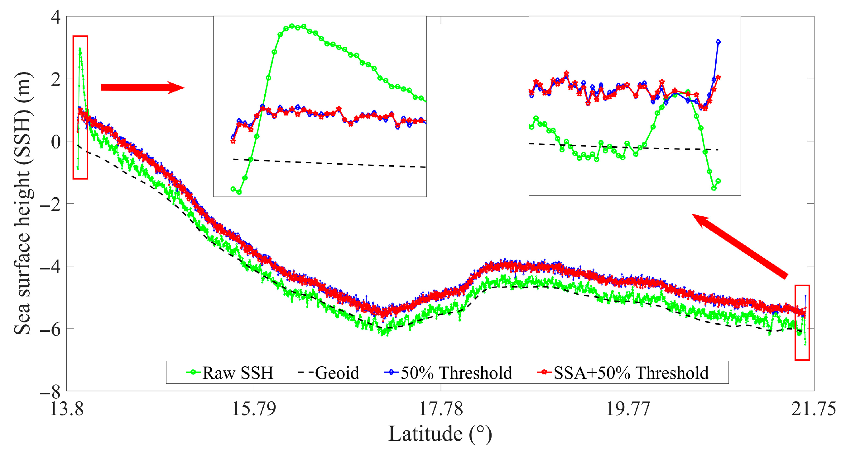
3.2. Comparison of Retracked SSHs

The 20-Hz waveforms data of the c340-p153 track were denoised using the SSA algorithm described earlier to obtain the SSA-denoised waveforms. Both the raw and SSA-denoised waveforms were retracked by the 50% threshold retracker, respectively. Figure 5 compares the raw SSH, the retracked SSHs from the 50% threshold, and SSA + 50% threshold retracker, respectively, with referenced geoidal heights calculated by the EGM2008 model. Here, the SSA + 50% threshold retracker refers to using the 50% threshold retracker for the SSA-denoised waveforms. As can be seen from Figure 5, the deviation of SSH from geoidal height increased as the tracks approached the land. In the coastal region, the retracked SSH profile was smoother than the raw SSH profile, and the former was more similar to the geoidal height than the latter.

The success of the retracker in producing a better SSH estimate value was identified by computing the standard deviations of the difference between SSHs and geoid heights, and the improvement percentage (IMP). The calculation formula of IMP is as follows [18].

$$\mathrm{IMP}=\frac{{\delta }_{\mathrm{raw}}-{\delta }_{\mathrm{retracked}}}{{\delta }_{\mathrm{raw}}}\times 100\%$$

(8)

where, ${\delta }_{\mathrm{raw}}$ and ${\delta }_{\mathrm{retracked}}$ are the standard deviations of the differences between raw SSHs and geoidal heights, and retracked SSHs and geoidal heights, respectively. The geoidal heights are calculated by EGM2008 model [24] in the present study.

The IMP was compared in three cases: (1) The entire c340-p153 track; (2) part of the c340-p153 track from land to ocean within 10 km from the coastline; and (3) part of the c340-p153 track from ocean to land within 10 km from the coastline.

Table 2. Standard deviations of differences between raw SSH, retracked SSH, and geoidal heights and improvement percentage (IMP).

The c340-p153 Track	Retracker	δraw (m)	δretracked (m)	IMP (%)
Entire track	50% threshold	0.2954	0.1587	46.27
	SSA + 50% threshold	0.2954	0.1519	48.57
Land to Ocean (Distance < 10 km)	50% threshold	0.8813	0.1170	86.73
	SSA + 50% threshold	0.8813	0.1164	86.80
Ocean to Land (Distance < 10 km)	50% threshold	0.1681	0.0900	46.47
	SSA + 50% threshold	0.1681	0.0690	58.99

shows the standard deviations (STDs) of the differences between raw SSH, retracked SSH, and geoidal heights and the IMP in these three cases. In Table 2, the STDs of differences between raw SSH and geoidal heights were smaller than that between the retracked SSH and geoidal heights. This means that waveform retracking iswas successful in improving the quality of altimeter data, especially in the coastal region. Whether in the open ocean or coastal region, the IMP values from the SSA + 50% threshold retracker were larger than those from the 50% threshold retracker. This indicates that SSA successfully improved the retracked SSHs estimate both in the open ocean and coastal region.

3.3. Comparison of Retracked SSHs Discrepancies at Crossover Points

SSA was used to reduce the noise information contained in the 20-Hz waveforms data of Jason-1 GM from cycle 500 to cycle 537 in the South China Sea to obtain the SSA-denoised waveforms, which was the same process as using SSA to denoise the waveforms of the c340-p153 track. Then, the 50% threshold retracker was used to retrack the raw and SSA-denoised waveforms.

There was an SSH difference at the crossover point between the ascending and descending tracks, e.g., Jason-1 GM ground tracks in Figure 1b. The crossover differences can be used to evaluate the quality of the retracked SSHs [10]. In order to compare the retracked SSHs from the 50% threshold retracker and that from the SSA + 50% threshold retracker quantitatively, the mean, STD, and root mean square (RMS) of the crossover differences were calculated (

Table 3. Statistical results of crossover differences between the retracked SSHs from the 50% threshold and SSA + 50% threshold retracker.

Distance	Retracker	Mean (m)	STD (m)	RMS (m)
d ≤ 10 km (2526)	50% threshold	0.0125	0.5052	0.5053
	SSA + 50% threshold	0.0059	0.4467	0.4466
d > 10 km (48,407)	50%threshold	−0.0007	0.2664	0.2664
	SSA + 50%threshold	−0.0002	0.2529	0.2529

). The statistical results were categorized into two classes, according to the nearest distances from the crossovers to land: Distances less than 10 km and greater than 10 km. The number in the brackets in column one indicates the number of crossovers in these two classes.

As can be seen from Table 3, the accuracy of the retracked SSHs in the coastal region (distances less than 10 km from the land) was lower than that in the open ocean (distances more than 10 km from the land). Regardless of whether the distance was more than 10 km or less than 10 km, both the STDs and RMSs from the SSA + 50% threshold retracker were smaller than those from the 50% threshold retracker, which shows that the retracked result of the SSA + 50% threshold retracker was better than that of the 50% threshold retracker. This indicates SSA can effectively improve the precision of the retracked SSHs, whether in the open ocean or coastal region. This conclusion is consistent with Section 3.2.

4. MSSH Model and Validation

4.1. MSSH Model from SSA-Denoised Waveform Retracked SSHs

All the 20-Hz waveforms data from Jason-1 SGDR products, including ERM1, ERM2, and GM in Table 1, were denoised with the SSA described earlier to obtain SSA-denoised waveforms, and the 50% threshold retracker was performed for these SSA-denoised waveforms to obtain the 20-Hz retracked SSHs. These 20-Hz retracked SSHs were compressed by linear regression to obtain 1-Hz retracked SSHs. In this linear regression, the SSHs over three-times larger than the STD were eliminated by an iterative outlier detection, and data with less than 10 points were also not considered. Then, these 1-Hz SSHs were used to establish an MSSH model over the South China Sea with grid of 2′ × 2′ (shows in Figure 6). The process of establishing MSSH model mainly includes data preprocessing, the removal of the temporal oceanic variability, crossover adjustment, and gridding, which has been detailed by Yuan et al. [25].

4.2. Validations

The MSSH model (shown in Figure 6) was called Model 1. The retracked SSHs by the 50% threshold retracker for the raw waveforms was also used to establish an MSSH model called Model 2. The fundament for both Model 1 and Model 2 was a seven-year (from 2002 to 2009) mean profile of Jason-1. The main difference between Model 1 and Model 2 was whether the SSA algorithm was used for noise reduction during data processing.

In order to validate the accuracy and reliability of the MSSH model established in the present study and whether SSA can effectively improve the accuracy of the MSSH model, Model 1 and Model 2 were compared in terms of SSHs with the CLS15 [26] and DTU18 [27] models in the South China Sea, respectively. CLS15 was published by the Collecte Localisation Satellites (CLS) and the French Centre National d’Etudes Spatiales (CNES), and DTU18 was released by the Technical University of Denmark (DTU). The fundament for CLS15 and DTU18 with a grid of 1′ × 1′ was a 20-year (from 1993 to 2012) mean profiles of T/P, Jason-1, and Jason-2. The difference between the MSS models depends on the dataset used for calculation and the data processing method [25].

Model 1 (represented by M1), Model 2 (represented by M2), CLS15 (represented by C), and DTU18 (represented by D) were compared in terms of SSHs with each other, as listed in

Table 4. Statistics on the differences between different MSS models (Model 1 and Model 2 were established using the retracked sea surface heights (SSHs) from the SSA + 50% threshold and 50% threshold retracker, respectively; M1 for Model 1; M2 for Model 2; C for CLS15; D for DTU18) (in m).

Model Discrepancy	M1-C	M2-C	M1-D	M2-D	M1-M2	C-D
Max	2.2095	2.1881	4.3607	4.3481	0.3909	4.5890
Min	−1.2853	−1.3391	−0.6792	−0.7294	−0.3536	−1.5820
Mean	0.1414	0.1281	0.1607	0.1474	0.0133	0.0193
STD	0.0698	0.0709	0.1179	0.1188	0.0141	0.1090
RMS	0.1577	0.1464	0.1993	0.1893	0.0194	0.1107
Number of points	325,951	325,951	325,951	325,951	325,951	325,951

. The table shows that means of Model 1 and Model 2 compared with CLS15 and DTU18 were obviously systematic biases. These systematic biases were mainly caused by two reasons: The differences between the SSHs measured by different altimetry satellites, and the impact of the oceanic variability. Both CLS15 and DTU18 were established from multi-satellite altimeter data, and these data were adjusted to have the same reference ellipsoid and frame as T/P. However, there was a systematic bias between the SSHs measured by T/P and those measured by Jason-1 of about 10.86 cm in the South China Sea [28]. These four models have different reference time periods: The reference periods of Model 1 and Model 2 span from 2002 to 2009, while the reference periods of CLS15 and DTU18 span from 1993 to 2012. Moreover, the sea level in the South China Sea showed an upward trend, with an increase rate of about 4.25 mm/yr [28,29].

The STDs of Model 1 and Model 2 compared with CLS15 were much smaller than those compared with DTU18, and the differences of STDs among CLS15, Model 1, and Model 2 were within 1 cm of DTU18. This indicates the high-degree consistency among Model 1, Model 2, and CLS15, and the obvious differences from DTU18. The STDs of Model 1 were smaller than those of Model 2, compared with CLS15 and DTU18.

These four models were compared in terms of SSH in the open ocean and coastal region (i.e., ~10 km from land), respectively, and the results are listed in

Table 5. Statistics on the differences between different MSS models (Model 1 and Model 2 were established using the retracked sea surface heights (SSHs) from the SSA + 50% threshold and 50% threshold retracker, respectively; M1 for Model 1; M2 for Model 2; C for CLS15; D for DTU18) in the open ocean and coastal region (in m).

Model Discrepancy		M1-C	M2-C	M1-D	M2-D	M1-M2	C-D
Coastal region	Max	1.8059	1.7862	4.3607	4.3481	0.3909	4.0920
	Min	−1.2853	−1.3391	−0.6792	−0.7294	−0.3536	−1.5820
	Mean	0.1173	0.1033	0.2125	0.1985	0.0140	0.0951
	STD	0.1521	0.1543	0.3215	0.3230	0.0262	0.3120
	RMS	0.1921	0.1857	0.3853	0.3791	0.0297	0.3262
	Number of points	31,257	31,257	31,257	31,257	31,257	31,257
Open ocean	Max	2.2095	2.1881	3.3181	3.3000	0.1403	4.5890
	Min	−1.2709	−1.2890	−0.3862	−0.4003	−0.3463	−1.4930
	Mean	0.1439	0.1308	0.1552	0.1420	0.0132	0.0112
	STD	0.0535	0.0545	0.0641	0.0651	0.0121	0.0461
	RMS	0.1536	0.1416	0.1679	0.1562	0.0179	0.0475
	Number of points	294,694	294,694	294,694	294,694	294,694	294,694

. The table shows that the STDs of Model 1 and Model 2 compared with CLS15 and DTU18 were 5~7 cm in the open ocean, whereas they rose up to the several decimeters in coastal region. Moreover, the STDs of Model 1 and Model 2 compared with DTU18 were almost twice of those compared with CLS15 in the coastal region. This indicates that DTU18 mainly differed from Model 1, Model 2, and CLS15 in coastal region, and it is assumed that this was mainly caused by the differences in the preprocessing of altimeter data. The STDs of the discrepancy between Model 1 and Model 2 were less than 2 cm in the open ocean and 3 cm in the coastal region. This indicates that these two models displayed more difference in the coastal region. In addition, the STDs of Model 1 compared with the two models CLS15 and DTU18 were lower than those of Model 2 compared with the two, indicating that the accuracy of Model 1 was superior to that of Model 2.

5. Conclusions

Altimeter waveforms are usually contaminated by land, island, sea reef, sea ice, seabed terrain, etc., which leads to incorrect SSHs retracked from these corrupted waveforms [30]. Moreover, the precision of MSSH model established from these poor SSHs is affected as well. SSA is a classical technique used in signal processing, and is also sometimes used in denoising signals. Therefore, it can be used to reduce the noise level in altimeter waveforms.

In this paper, the c340-p153 track of Jason-1 from 13.80° N to 21.75° N was selected as the experimental object to introduce the specific process of SSA to reduce the noise level in altimeter waveforms. All waveforms data of Jason-1 from 2002 to 2013 (including ERM1, ERM2 and GM) were processed by SSA noise reduction to obtain SSA-denoised waveforms, which were retracked by a 50% threshold retracker to obtain corresponding retracked SSHs. Then, these retracked SSHs were used to establish MSSH model over South China Sea with grid of 2′ × 2′.

A comparison of the IMP and statistical results of crossover differences of the retracked SSHs from the SSA + 50% threshold retracker and those from the 50% threshold retracker showed that the SSA allowed a noise reduction on the Jason-1 altimeter waveforms, and can successfully improve the accuracy of retracked SSHs either in the open ocean or coastal region.

Model 1 and Model 2 were compared with CLS15 and DTU18 in the South China Sea, and the results showed that these four models had a high-degree consistency. Moreover, Model 1 showed higher accuracy than Model 2, and the main difference between these two models was found mainly in the coastal region. This result indicates that using SSA to reduce the noise level of the Jason-1 altimeter waveforms can effectively improve the accuracy of the MSSH model.

The SSA algorithm was used to denoise the waveforms of Jason-1 to establish an MSSH model over the South China Sea. It can also be employed to denoise other satellite altimeter waveforms to establish MSSH models of other regions, even a global MSSH model, which is our main aim for the next study.

References

1. Quartly, G.; Chen, G. Introduction to the Special Issue on “Satellite Altimetry: New Sensors and New Applications”. Sensors 2006, 6, 616–619. [Google Scholar] [CrossRef] [Green Version]
2. Guo, J.; Gao, Y.; Hwang, C.; Sun, J. A multi-subwaveform parametric retracker of the radar satellite altimetric waveform and recovery of gravity anomalies over coastal oceans. Sci. China Earth Sci. 2010, 53, 610–616. [Google Scholar] [CrossRef]
3. Hernandez, F.; Schaeffer, P. The CLS01 Mean Sea Surface: A Validation with the GSFC00.1 Surface; CLS: Ramonville St Agne, France, 2001. [Google Scholar]
4. Hwang, C.; Hsu, H.-Y.; Jang, R. Global mean sea surface and marine gravity anomaly from multi-satellite altimetry: Applications of deflection-geoid and inverse Vening Meinesz formulae. J. Geodesy 2002, 76, 407–418. [Google Scholar] [CrossRef]
5. Fu, L.L.; Cazenave, A. Satellite Altimetry and Earth Sciences: A Handbook of Techniques and Applications; Academic Press: San Diego, CA, USA, 2001. [Google Scholar]
6. Deng, X. Improvement of Geodetic Parameter Estimation in Coastal Regions from Satellite Radar Altimetry. Ph.D. Thesis, Curtin University of Technology, Perth, Australia, 2003. [Google Scholar]
7. Deng, X.; Featherstone, W.E. A coastal retracking system for satellite radar altimeter waveforms: Application to ERS-2 around Australia. J. Geophys. Res. Oceans 2006, 111. [Google Scholar] [CrossRef] [Green Version]
8. Gommenginger, C.; Thibaut, P.; Fenodlio-Marc, L.; Quartly, G.; Deng, X.; Gomez-Enri, J.; Challenor, P.; Gao, Y. Retracking Altimeter Waveforms Near the Coasts. In Coastal Altimetry; Vignudelli, S., Kostianoy, A.G., Cipollini, P., Benveniste, J., Eds.; Springer: Berlin/Heidelberg, Germany, 2011; pp. 61–102. [Google Scholar]
9. Deng, X.; Featherstone, W.E.; Hwang, C.; Berry, P.A.M. Estimation of Contamination of ERS-2 and POSEIDON Satellite Radar Altimetry Close to the Coasts of Australia. Mar. Geod. 2002, 25, 249–271. [Google Scholar] [CrossRef]
10. Yang, L.; Lin, M.; Pan, D. Retracking Jason1 Altimeter Waveform Over Chinacoastal Zone. In Proceedings of the SPIE-Microwave Remote Sensing of the Atmosphere and Environment VI, Noumea, New Caledonia, 19 November 2008; Volume 7154. [Google Scholar]
11. Idris, N.H.; Deng, X. The Retracking Technique on Multi-Peak and Quasi-Specular Waveforms for Jason-1 and Jason-2 Missions near the Coast. Mar. Geod. 2012, 35, 217–237. [Google Scholar] [CrossRef] [Green Version]
12. Vautard, R.; Yiou, P.; Ghil, M. Singular-spectrum analysis: A toolkit for short, noisy chaotic signals. Physica D 1992, 58, 95–126. [Google Scholar] [CrossRef]
13. Golyandina, N.; Zhigljavsky, A. Singular Spectrum Analysis for Time Series; Springer: New York, NY, USA, 2013. [Google Scholar]
14. Shen, Y.; Guo, J.; Liu, X.; Kong, Q.; Guo, L.; Li, W. Long-term prediction of polar motion using a combined SSA and ARMA model. J. Geodesy 2018, 92, 333–343. [Google Scholar] [CrossRef]
15. Guo, J.; Shi, K.; Liu, X.; Sun, Y.; Li, W.; Kong, Q. Singular spectrum analysis of ionospheric anomalies preceding great earthquakes: Case studies of Kaikoura and Fukushima earthquakes. J. Geodyn. 2019, 124, 1–13. [Google Scholar] [CrossRef]
16. CNES. Jason-1 Products Handbook; SALP-MU-M5-OP-13184-CN; Issue: 5 Rev 1; CNES: Paris, France, 2016. [Google Scholar]
17. Yang, L.; Lin, M.; Liu, Q.; Pan, D. A coastal altimetry retracking strategy based on waveform classification and sub-waveform extraction. Int. J. Remote Sens. 2012, 33, 7806–7819. [Google Scholar] [CrossRef]
18. Hwang, C.; Guo, J.; Deng, X.; Hsu, H.-Y.; Liu, Y. Coastal Gravity Anomalies from Retracked Geosat/GM Altimetry: Improvement, Limitation and the Role of Airborne Gravity Data. J. Geodesy 2006, 80, 204–216. [Google Scholar] [CrossRef]
19. Guo, J.; Hwang, C.; Chang, X.; Liu, Y. Improved threshold retracker for satellite altimeter waveform retracking over coastal sea. Prog. Nat. Sci. 2006, 16, 732–738. [Google Scholar]
20. Ganguly, D.; Chander, S.; Desai, S.; Chauhan, P. A Subwaveform-Based Retracker for Multipeak Waveforms: A Case Study over Ukai Dam/Reservoir. Mar. Geod. 2015, 38, 581–596. [Google Scholar] [CrossRef]
21. Davis, C.H. Growth of the Greenland ice sheet: A performance assessment of altimeter retracking algorithms. IEEE Trans. Geosci. Remote 1995, 33, 1108–1116. [Google Scholar] [CrossRef]
22. Davis, C.H. A robust threshold retracking algorithm for measuring ice-sheet surface elevation change from satellite radar altimeter. IEEE Trans. Geosci. Remote 1997, 35, 974–979. [Google Scholar] [CrossRef]
23. Uebbing, B.; Kusche, J.; Forootan, E. Waveform retracking for improving level estimations from topex/poseidon, Jason-1, and Jason-2 altimetry observations over african lakes. IEEE Trans. Geosci. Remote 2015, 53, 2211–2224. [Google Scholar] [CrossRef]
24. Pavlis, N.K.; Holmes, S.A.; Kenyon, S.C.; Factor, J.K. The development and evaluation of the Earth Gravitational Model 2008 (EGM2008). J. Geophys. Res. 2012, 117, B04406. [Google Scholar] [CrossRef] [Green Version]
25. Yuan, J.; Guo, J.; Liu, X.; Zhu, C.; Niu, Y.; Li, Z.; Ji, B.; Ouyang, Y. Mean sea surface model over China seas and its adjacent ocean established with the 19-year moving average method from multi-satellite altimeter data. Cont. Shelf Res. 2020, 192, 104009. [Google Scholar] [CrossRef]
26. Pujol, M.-I.; Schaeffer, P.; Faugère, Y.; Raynal, M.; Dibarboure, G.; Picot, N. Gauging the improvement of recent mean sea surface models: A new approach for identifying and quantifying their errors. J. Geophys. Res. Oceans 2018, 123, 5889–5911. [Google Scholar] [CrossRef]
27. Andersen, O.; Knudsen, P.; Stenseng, L. A New DTU18 MSS Mean Sea Surface—Improvement from SAR Altimetry. In Proceedings of the 25 Years of Progress in Radar Altimetry Symposium, Portugal, Duration, 24–29 September 2018. [Google Scholar]
28. Guo, J.; Wang, J.; Hu, Z.; Hwang, C.; Chen, C.; Gao, Y. Temporal-spatial variations of sea level over Chinese seas derived from altimeter data of TOPEX/Poseidon, Jason-1 and Jason-2 from 1993 to 2012. Chin. J. Geophys. 2015, 58, 3103–3120. [Google Scholar]
29. Guo, J.; Hu, Z.; Wang, J.; Chang, X.; Li, G. Sea level change of China seas and neighboring ocean based on satellite altimetry missions from 1993 to 2012. J. Coast. Res. 2015, 73, 17–21. [Google Scholar] [CrossRef]
30. Huang, Z.; Wang, H.; Luo, Z.; Shum, C.K.; Tseng, K.-H.; Zhong, B. Improving Jason-2 Sea Surface Heights within 10 km Offshore by Retracking Decontaminated Waveforms. Remote Sens. 2017, 9, 1077. [Google Scholar] [CrossRef]
Figure 1. The ground tracks map of Jason-1 in South China Sea. (a) The ground tracks map of ERM1 and ERM2. The number 153 is the pass number, the green lines are the ERM1 ground tracks, and the blue lines are the ERM2 ground tracks; (b) the ground tracks map of the geodetic mission (GM).
Jmse 08 00426 g001
Figure 2. Processing flowchart of Jason-1 waveforms.
Jmse 08 00426 g002
Figure 3. Ratio of the eigenvalues.
Jmse 08 00426 g003
Figure 4. Beginning part of the raw waveform series, the SSA-denoised waveform series, and corresponding residual series defined as the difference between the raw and SSA-denoised waveform series. (a) Raw waveform series and SSA-denoised waveform series; (b) residual series.
Jmse 08 00426 g004
Figure 5. Comparison of raw SSH, retracked SSH, and referenced geoid height (calculated by EGM2008 model) along the track of Jason-1 cycle340 pass153.
Jmse 08 00426 g005
Figure 6. Mean sea surface height (MSSH) model over the South China Sea from the SSHs of the SSA-denoised waveform retracking of Jason-1.
Jmse 08 00426 g006