Research on Risk Evaluation and Dynamic Escape Path Planning Algorithm Based on Real-Time Spread of Ship Comprehensive Fire

Abstract

As an independent building entity on the sea, the ship has a large number of internal electrical equipment and a compact space structure, which is prone to fire. This paper proposes a key technology of virtual dynamic escape of ships based on the fire spread prediction model for research. Taking the 63,500 DWT(Dead Weight Tonnage) tanker cabin as a research entity, the mathematical and physical models of ship fire simulation are established. Through the graphical analysis of the experimental data of the fire spread simulation, the temperature, CO concentration, and smoke concentration change rules under different working conditions at the fixed detection point position are obtained. Then, based on temperature, CO concentration and smoke concentration three impact factors, set up a comprehensive fire real-time situational risk evaluation index system. Using the MATLAB software, based on the principle of the fuzzy neural network fire ship’s integrated real-time situational risk evaluation model structure design and simulation test, obtained the corresponding training to comprehensive risk evaluation model of the network. Generate navigation grid according to the law of fire sprawl, and plan escape path. The traditional A* algorithm is improved, and an example is used to prove that the path-finding result after the improved algorithm is shorter than the path found by the traditional algorithm, which meets the path-finding requirements in a three-dimensional environment.

1. Introduction

There are a large number of sea freight and passenger ships traveling each year. As an independent individual, the ship has a compact internal structure compared to road buildings; the circuit equipment problems are likely to cause fires, and the fire incidence is high. Therefore, marine fire escape is very important [1,2].

Evacuation path planning is of significant importance to safely and efficiently evacuate occupants inside public buildings [3,4]. Some scholars have conducted fire analysis on shipbuilding [5].It is necessary to understand the laws of ship fire spread through the research on the characteristics of fire spread, and obtain relevant environmental information, so as to construct a dynamically changing fire scene [6,7].

In 2017, Ryu Eun-Gyong and Yang Chan-Su [8] conducted basic research on the escape guidance system of passenger ships, and used the developed situation-aware escape navigation system to conduct escape experiments on the training ship. The experiments show that the system can effectively shorten the escape time. Bin Wang [9] and others proposed a fire emergency rescue environment simulation based on the Building Information Modeling (BIM) model in 2014 to complete the corresponding path planning. In 2017, Qing Xiong [10] et al. studied the dynamic indoor environment evacuation, proposed three dynamic indoor field models for the establishment of the evacuation space model, and combined the real-time dynamic information to simulate the emergency rescue process;

Escape path planning is the key to fire escape rescue [11]. In 2017, Chenghua Ou, Chaochun Li [12], and others, used three-dimensional (3D) visualization technology to establish an underground drainage visualization management system for the horizontal well level of the mining area. In 2019, Hao Wu and Jiandong Yang [13], and others, conducted research on the ship’s firefighting training system, using virtual reality technology to build firefighting equipment operation emergency training modules, emergency rescue, and adaptive training. However, their research still has limitations. This paper uses fuzzy theory to study escape routes, fuzzy neural networks are mainly used in UAV(Unmanned Aerial Vehicle) and other fields, but there are few studies on fire protection, this article is based on ship fire, using fuzzy neural network to more accurately record the fire source information [14,15]. This paper uses software simulation analysis to determine the law of fire-related spread, and establishes a risk assessment system based on this, and uses software to design and simulate the comprehensive fire spread situation risk assessment based on fuzzy neural network.

For path planning, the first step is to construct a virtual scene. The traditional methods mainly include grid method, quadtree method, visible point method, etc., but there are many restrictions on the planning space [16,17,18,19]. This article chooses the navigation grid method, which is the primary method for map representation of the complex path environment [20]. The navigation grid method simplifies the three-dimensional space into two-dimensional space, and divides the scene map into regular graphics, which can be used to record the walkable areas in the scene and express the path intuitively [21].

The A* algorithm is an effective direct search method for solving the shortest path in a static road network. It quickly locks the target direction through the heuristic information contained in the evaluation function. It is also the most used path planning algorithm [22]. In 2016, Suqiong Chen [23] improved the path finding efficiency of game maps by improving the A* algorithm; in 2017, Yajie Wu [24], and others, conducted research on robot path planning based on the A* algorithm. In 2019, Hailiang Jin [25] and others improved the A* path planning algorithm in response to the problem of congestion of fire escape personnel in high-rise complex buildings. This paper proposes an escape map representation method that dynamically updates the navigation grid based on the comprehensive fire spread situation, and based on this navigation grid map combined with the improved A* pathfinding algorithm, and conduct experimental verification.

2. Analysis of Fire Spread in Ship Cabin

Mastering the spread of fire in ship cabins is the key to building a fire information field, and it is also a prerequisite for planning escape routes. After a fire, a large amount of smoke will be generated in a relatively closed environment. The threat factors for people in the fire are generally reflected in three aspects: temperature, visibility, and toxic gases (CO, CO₂, etc.). Based on these three main influencing factors, a fire simulation model was established to analyze the influencing factors.

2.1. Establishment of a Simplified Model of the Cabin

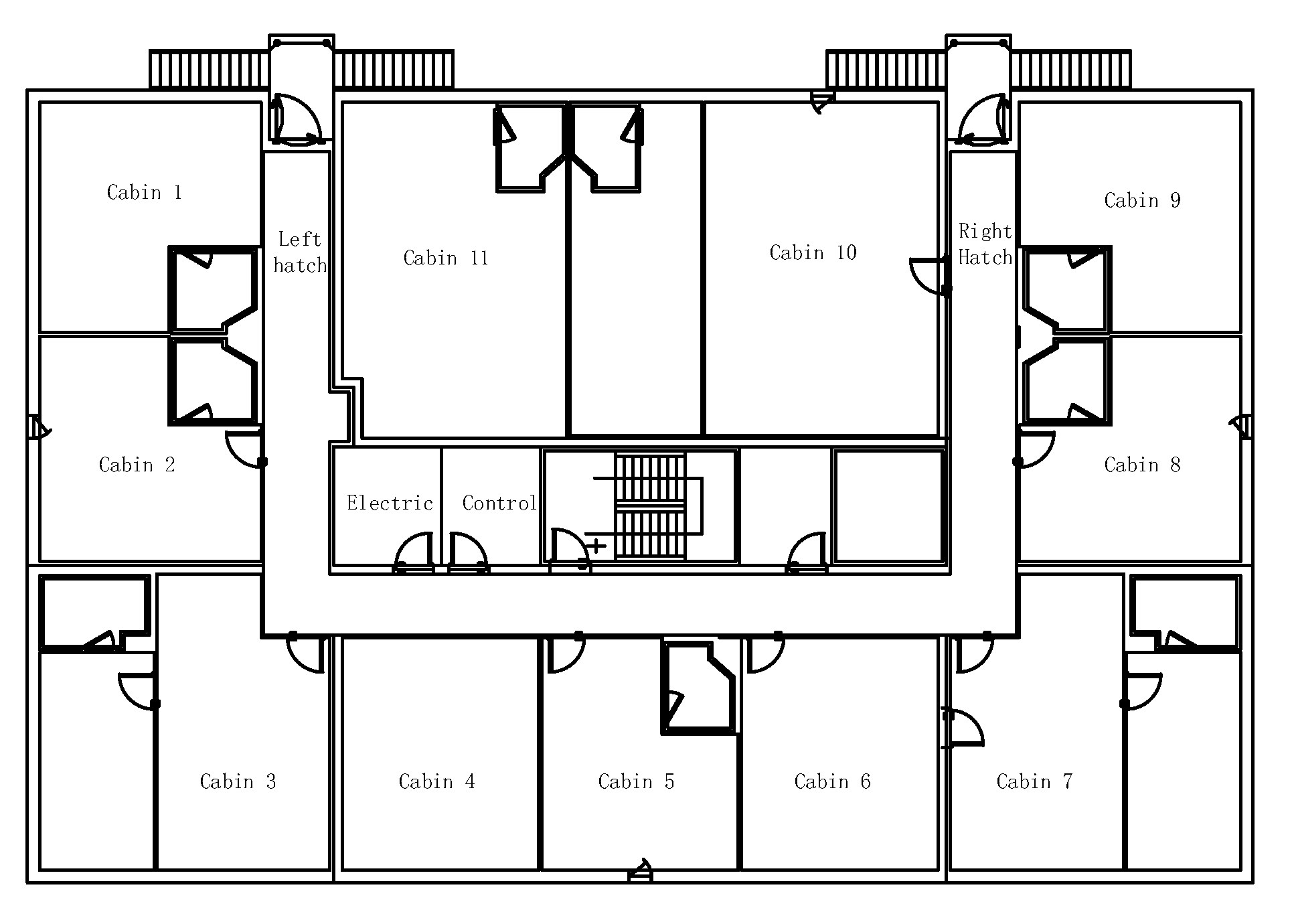
The research object of this paper is 63,500 DWT oil tanker. The deck in the daily life area is selected as the research deck. At present, ultra-fine modeling cannot be completed in fire simulation software, and in the fire spread simulation calculation, smaller equipment has little effect on the corresponding flow field calculation in the simulation, so the cabin structure is simplified to obtain a reasonable cabin model. 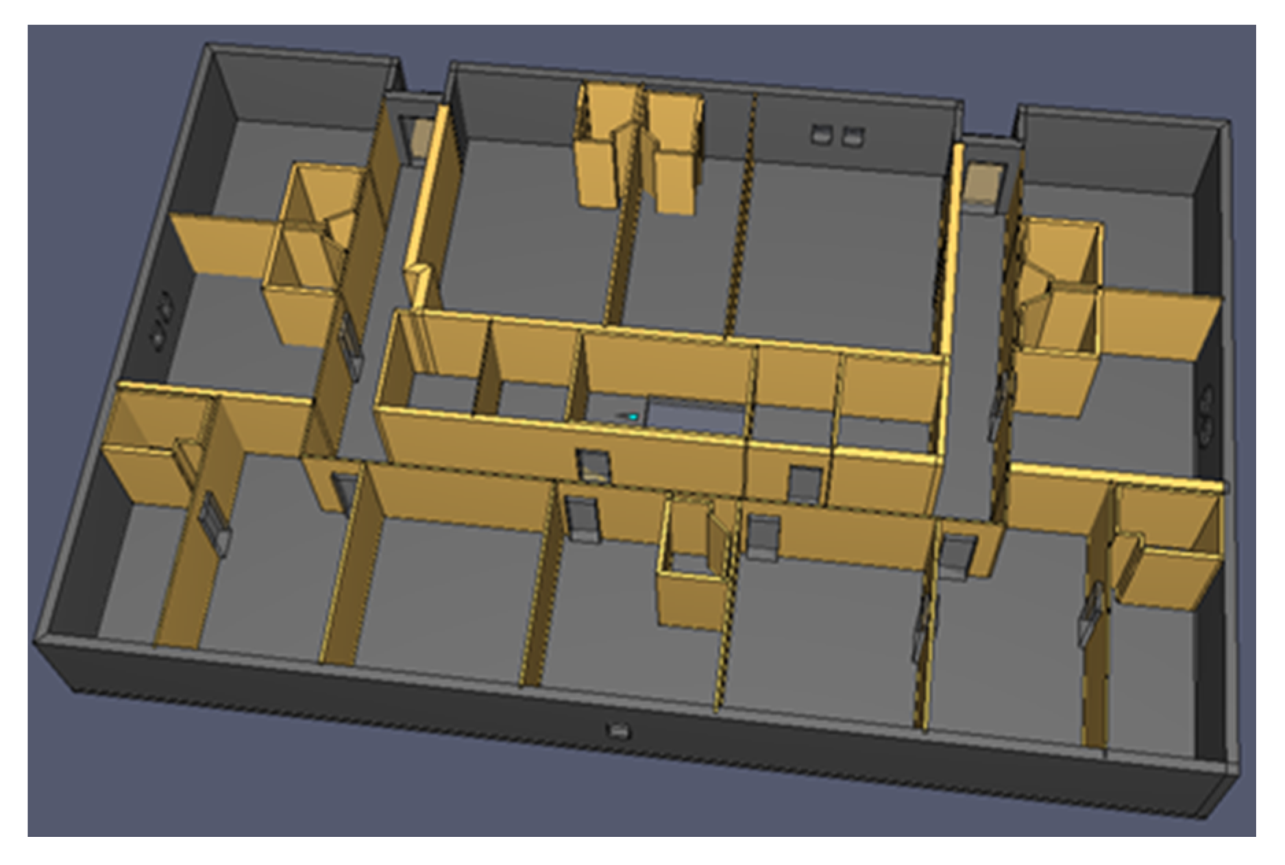Figure 1 is a simplified deck plan. In order to simulate actual living conditions, the cabin doors and cabin windows are set to open. Build a 1:1 three-dimensional cabin model in PyroSim, according to the drawings, as shown in Figure 2.

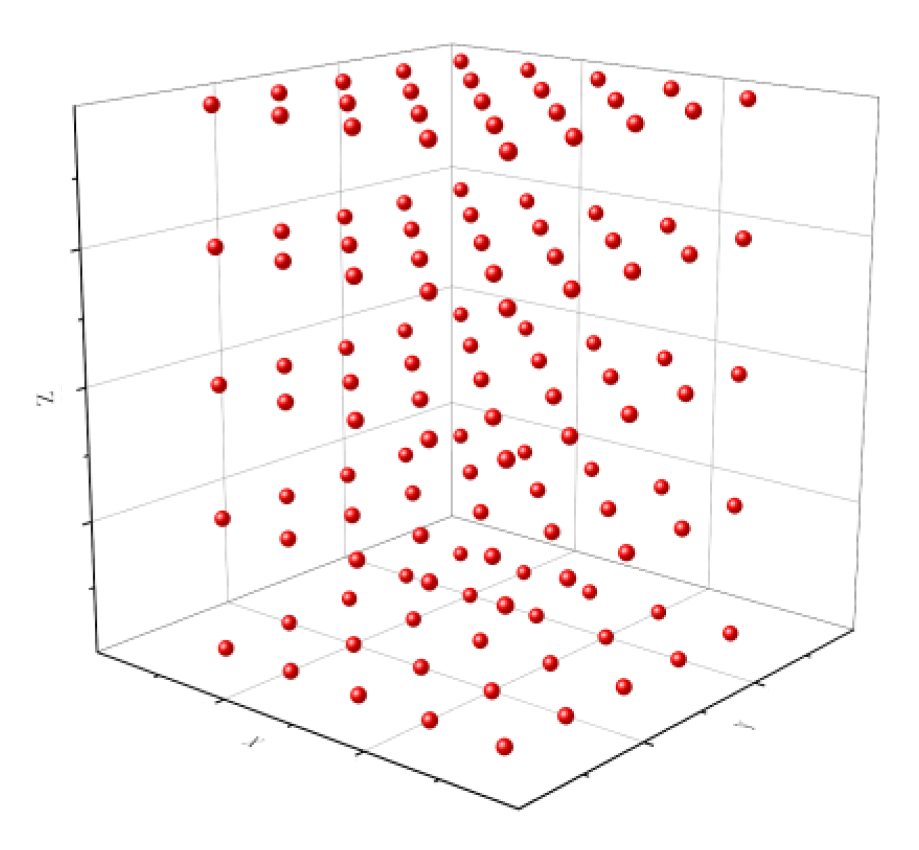
In order to obtain the environmental data of each point of the cabin in the simulation, it is necessary to arrange the measuring points in the simulation environment, set the distance between the measuring points to be equal, cover the entire simulation area, and set a thermocouple, smoke concentration, and CO concentration detector for each position. It is also necessary to, respectively, measure the temperature, smoke concentration, and CO concentration data of each point, and place the measurement points in the coordinate system. The layout diagram is shown in Figure 3.

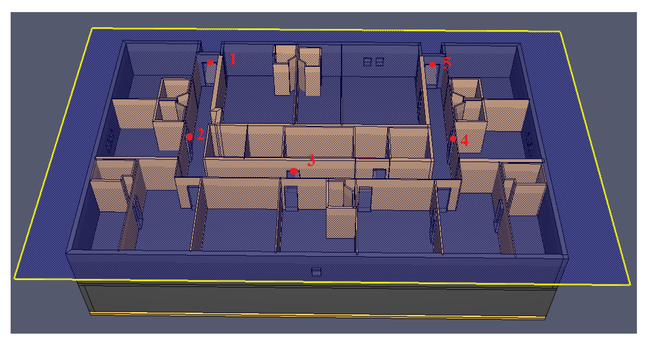
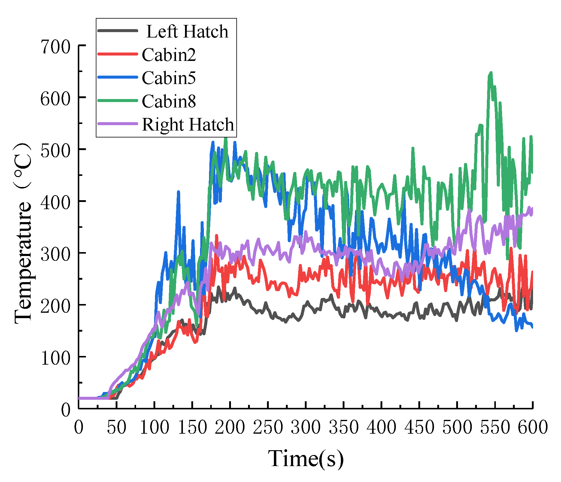
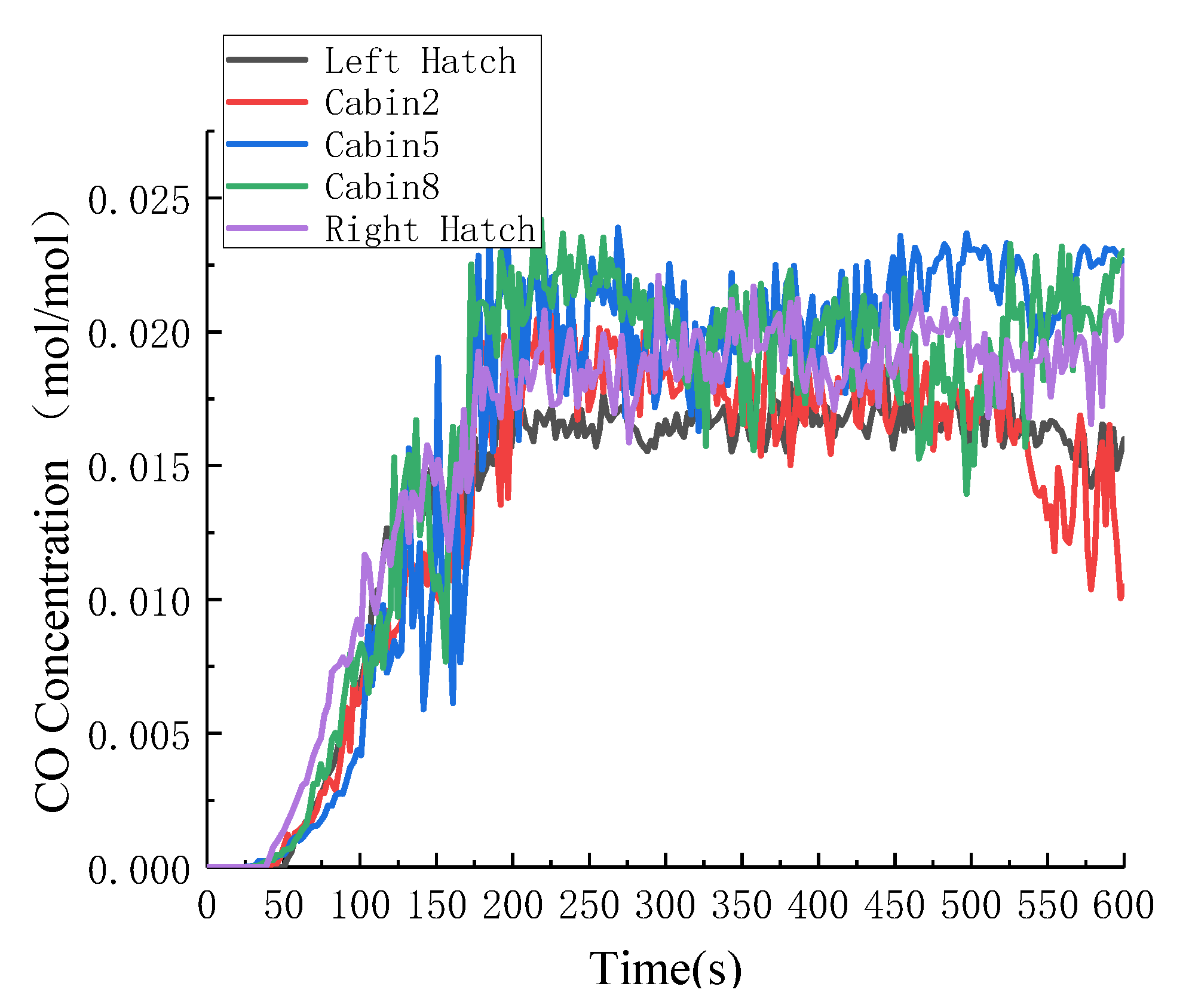
In order to intuitively understand the general law of fire spread, select five positions of the left hatch, cabin 2, cabin 5, cabin 8, and right hatch as key measurement points, as shown in Figure 4. After setting the relevant initial parameters, the calculation model can output the position of each measuring point and the relevant temperature, smoke concentration, and CO concentration data at each time of each measuring point, all of which are saved in the form of text and numerical values [26].

2.2. Analysis on the Law of Fire Spread in Ship Cabin

The temperature curve of the cabin fire simulation temperature is shown in Figure 5. It can be seen from the figure that the temperature at the five locations did not change much during the period before 50 s. After 50 s, the overall temperature change showed a rapid upward trend. When it reaches 150 s (the source of heat reaches the maximum heat release rate), the rate of temperature increase slows down and will fluctuate within a certain range after a period of time. The temperature at the exit of the staircase showed a downward trend for some time after 150 s, this is because the stairway is connected to the lower deck, and the smoke diffuses to the lower deck, so the trend of temperature change is different from the other four places.

The smoke concentration change curves of the five detection points are shown in Figure 6. From the figure, it can be seen that the overall smoke concentration change trend of the five positions is similar to the temperature change law. During the period when the fire started, there was no obvious change in each position. From about 50 s to 150 s, it showed a rapid upward trend, and maintained a period of continuous growth after 150 s. After 150 s, maintain a relatively stable state. The farther away from the fire source point, the rate of change is slower and the value is lower, which is in line with the actual situation.

The change curve of CO concentration at five detection points is shown in Figure 7. As the smoke concentration and CO concentration have a direct influence relationship, it can be seen from the figure that the overall trend of CO concentration change is similar to the smoke concentration.

According to the temperature, smoke concentration and CO concentration change curve in the cabin at different times; it can be sorted and analyzed, which can be used for fire spreading situation risk assessment and path planning.

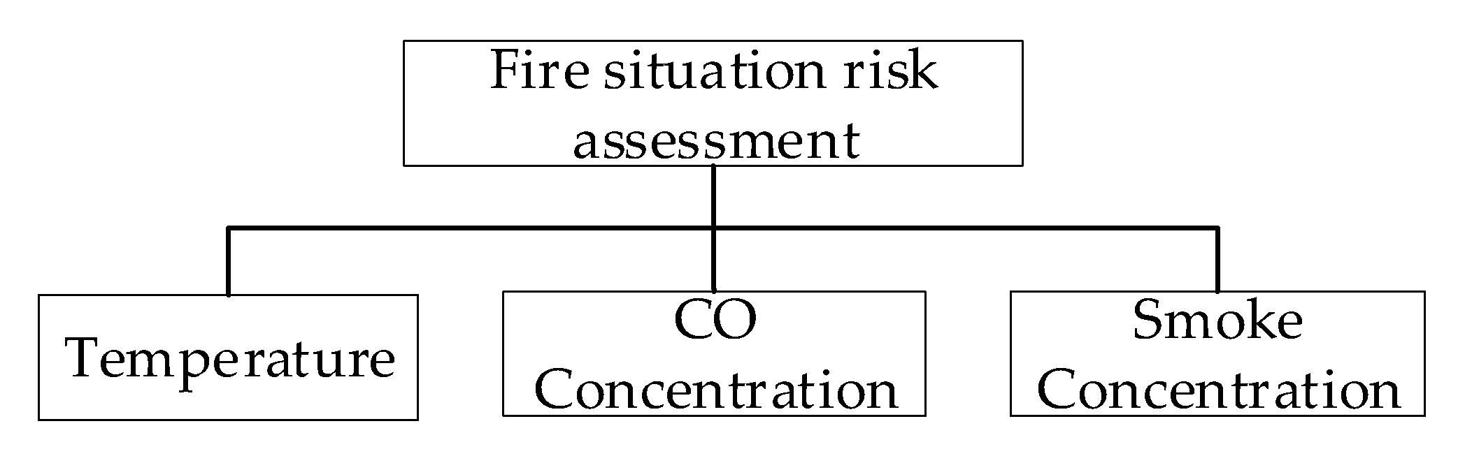
3. Comprehensive Fire Situation Risk Assessment Index System

The most critical step in risk evaluation is to establish a scientific, comprehensive, and effective evaluation index system. Once an indoor fire occurs, the spread rate is very fast. The threat factors of smoke to people in the fire are generally reflected in three aspects: high temperature, low visibility, and toxic gases. The low visibility is reflected in the smoke density.

Therefore, three environmental impact factors are selected to form a risk assessment system for the spread of fire in a certain area. The system diagram is shown in Figure 8.

According to the literature survey and the rich experience of the relevant ship engine room fire research experts, the classification standards for real-time fire situation risk assessment indicators are determined as shown in

Table 1. Classification standards of fire risk assessment indicators.

Index/Level	I (Safety)	II (A little safe)	III (Danger)	IV (Very Dangerous)
Temperature (°C)	<42	42–65	65–93	>93
CO Concentration 10−6 (mol/mol)	<200	200–800	800–3200	>3200
Smoke Concentration 10−6 (mol/mol)	<500	500–1000	1000–3800	>3800

:

4. Model of Real-Time Fire Risk Assessment Based on Fuzzy Neural Network

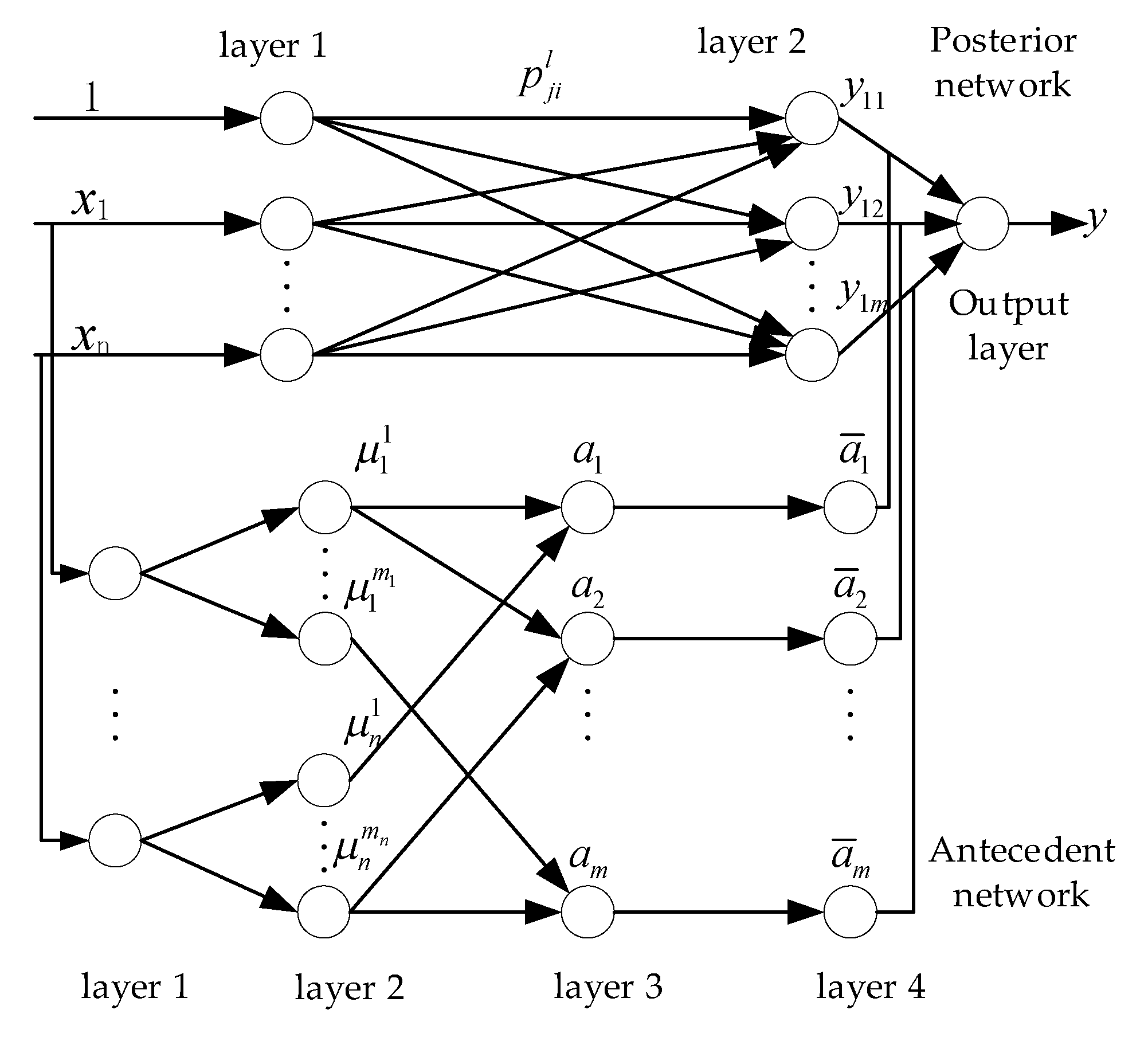
4.1. Structural Design of Fuzzy Neural Network

Using fuzzy neural network structure based on the Takagi-Sugeno(T-S) type, the fuzzy neural network of the Takagi-Sugeno(T-S) architecture has a simple structure, and the reasoning ability of the fusion fuzzy theory, and the learning ability of the neural network, do not have a strong global approximation ability [27]. The structural design is shown in Figure 9.

The network is composed of two parts: the antecedent and the posterior network. The antecedent network is divided into four layers. The first layer is the input layer; input the influence factor training sample $x={\left(x_1,x_2,\dots ,x_n\right)}^T$. In this paper, temperature, CO concentration, and smoke concentration values are input as parameters, so the number of nodes here is three.

The second layer is a fuzzy layer. Each node $x_i$ of the first layer corresponds to the i-th group of nodes in the second layer. Each group of nodes represents the corresponding membership degree, which is represented by a membership function. Use Gaussian function calculation:

$${\mu }_i^j={\mu }_{A_i^j}\left(x_i\right)=\exp \left(-{\left(\frac{x_i-c_{ij}}{{\sigma }_{ij}}\right)}^2\right)$$

(1)

$c_{ij}$ and ${\sigma }_{ij}$ are the center and width of the membership function, respectively, corresponding to three nodes in the first layer, each node corresponds to a set of 3membership functions in the second layer, so there are nine nodes in the second layer.

The third layer is the fuzzy rules layer, each node represents a rule, used to match the antecedent of the fuzzy rules, and calculate the applicability of each rule. The impact factor variable is 3, the number of membership functions in each group is 3, and the number of nodes in this layer is 3³ = 27:

$$a_i=\min \left({\mu }_1^{i_1},{\mu }_2^{i_2},\dots ,{\mu }_n^{i_n}\right)$$

(2)

The fourth layer is the normalization layer, and the number of nodes is the same as that of the third layer, which is 64, which realizes the normalization calculation:

$${\overline{a}}_i=\frac{a_i}{{\displaystyle \sum _{i=1}^m{a}_i}}i=1,2,\dots ,m$$

(3)

The first layer of the posterior network is the output layer, and the input value of the 0th node is 1, which is to provide the constant term of the posterior fuzzy rules for later calculation. The second layer is to calculate the aftermath of each fuzzy rule:

$$y_{ij}=p_{j0}^l+p_{j1}^l{x}_1+\cdot \cdot \cdot +p_{jn}^l{x}_n={\displaystyle \sum _{i=0}^n{p}_{ji}^l}{x}_i$$

(4)

In the formula, $j=1,2,\dots ,m;i=1,2,\dots ,n;l=1,2,\dots ,r$. The third layer is the anti-fuzzification process and calculates the system output value:

$$y_i={\displaystyle \sum _{j=1}^m{\overline{a}}_j}{y}_{ij}$$

(5)

4.2. System Learning Algorithm of Fuzzy Neural Network

The advantage of fuzzy neural network is to use the characteristics of self-learning to continuously learn and adjust the weights and thresholds in the model through training samples, so as to obtain the functions that meet the actual needs. Because the number of fuzzy divisions for each input is determined, the main learning parameters are the connection weight $p_{ji}^l$ of the posterior network and the center value $c_{ij}$ and width ${\sigma }_{ij}$ of the membership function in the antecedent network. The error function is:

$$E=\frac{1}{2}{\displaystyle \sum _{i=1}^r\left(t_i-y_i\right)}$$

(6)

In the above formula, $t_i$ and $y_i$ are the expected output and actual output, respectively. The learning algorithm for the coefficient $p_{ji}^l$ is:

$$\frac{\partial E}{\partial p_{ji}^l}=\frac{\partial E}{\partial y_1}\frac{\partial y_1}{\partial y_{ij}}\frac{\partial y_{ij}}{\partial p_{ji}^l}=-\left(t_i-y_i\right){\overline{a}}_j{x}_i$$

(7)

$$p_{ji}^l\left(k+1\right)=p_{ji}^l\left(k\right)-\beta \frac{\partial E}{\partial p_{ji}^l}=p_{ji}^l\left(k\right)+\beta \left(t_i-y_i\right){\overline{a}}_j{x}_i$$

(8)

The central value $c_{ij}$ and the width value ${\sigma }_{ij}$ of the membership function are calculated, the coefficient $p_{ji}^l$ is fixed first, and the back propagation (BP) algorithm is used:

$${\sigma }_i^{(5)}=t_i-y_i\left(i=1,2,\dots ,n\right)$$

(9)

$${\sigma }_j^{(4)}={\displaystyle \sum _{i=1}^r{\sigma }_i^{(5)}{y}_{ij}\left(j=1,2,\dots ,m\right)}$$

(10)

$${\sigma }_j^{(3)}={{\sigma }_i^{(4)}{\displaystyle \sum _{\begin{array}{l}i=1\\ i\ne j\end{array}}^m{a}_i}/\left({\displaystyle \sum _{i=1}^m{a}_i}\right)}^2\left(j=1,2,\dots ,m\right)$$

(11)

$${\sigma }_{ij}^{(2)}={\displaystyle \sum _{j=1}^m{\sigma }_j^{(3)}{s}_{ij}{e}^{-\frac{{\left(x_i-c_{ij}\right)}^2}{{\sigma }_{ij}^2}}}$$

(12)

when and performs a small operation, that is, ${\mu }_i^j$ is the minimum value input by the jth rule node, $s_{ij}=1$, otherwise $s_{ij}=0$. Finally get:

$$\frac{\partial E}{\partial c_{ij}}=-{\sigma }_{ij}^{(2)}\frac{2\left(x_i-c_{ij}\right)}{{\sigma }_{ij}}$$

(13)

$$\frac{\partial E}{\partial {\sigma }_{ij}}=-{\sigma }_{ij}^{(2)}\frac{2{\left(x_i-c_{ij}\right)}^2}{{\sigma }_{ij}}$$

(14)

$$c_{ij}\left(k+1\right)=c_{ij}\left(k\right)-\beta \frac{\partial E}{\partial c_{ij}}$$

(15)

$${\sigma }_{ij}\left(k+1\right)={\sigma }_{ij}\left(k\right)-\beta \frac{\partial E}{\partial c_{ij}}$$

(16)

In the above formula, $\beta >0$, is the learning rate.

4.3. Determination of Membership Function

It is used to express the mathematical way of fuzzy sets, the only constraint is that the value range is [0, 1]. Use the assignment method to select the membership function according to the actual situation, and use the linguistic variables in the fuzzification process. According to the definition of 2.1 evaluation index security level, relevant linguistic variables, and membership functions are established.

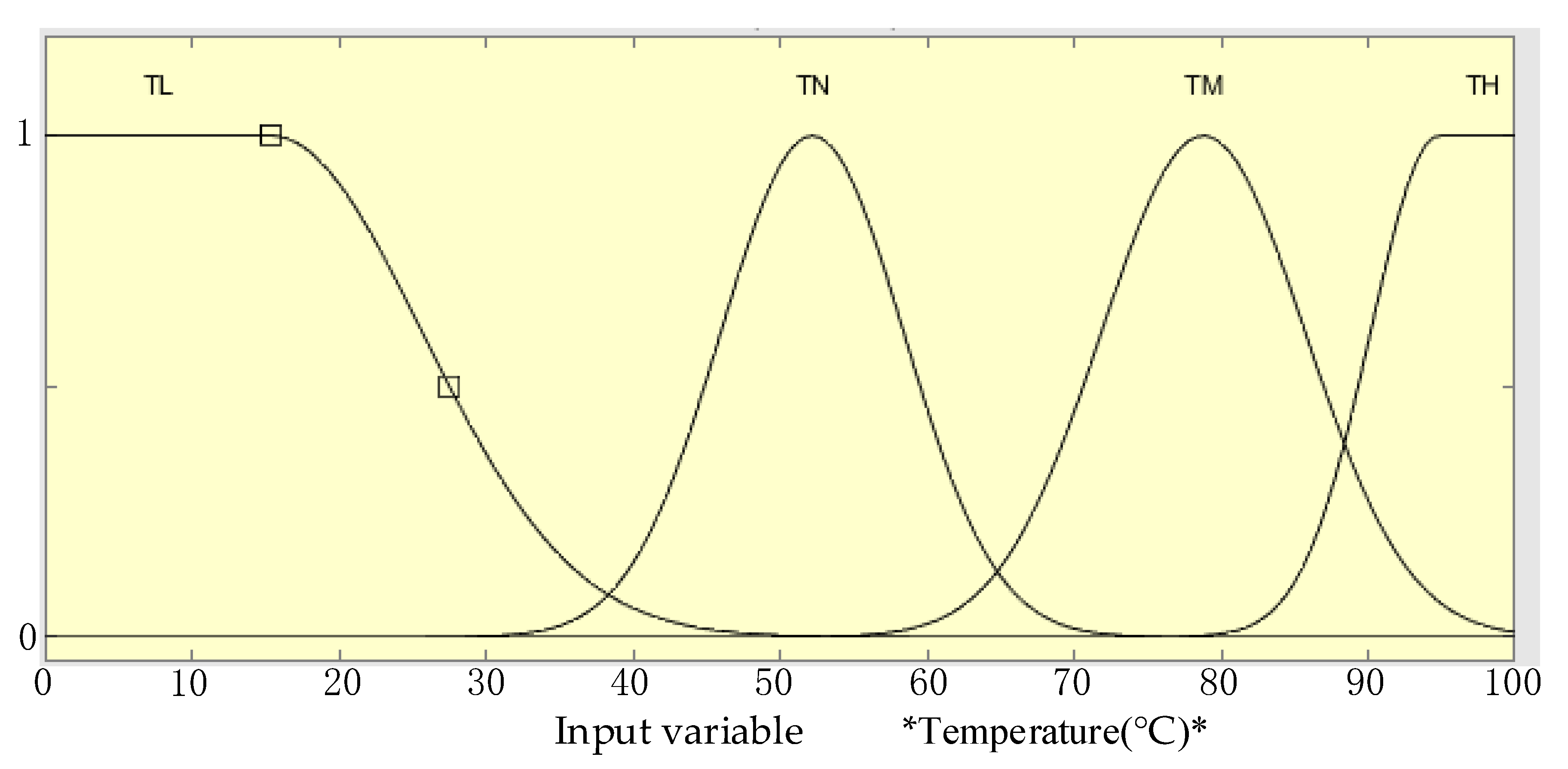
The influence factor temperature is the most direct indicator of fire anomaly detection. According to experience and expert analysis, the domain of determining temperature is [0, 100]. The unit is °C. It is divided into four levels, which can be expressed as temperature $\in \left\{TL,TN,TM,TH\right\}$, indicates that the temperature gradually increases. Its membership function is shown in Figure 10.

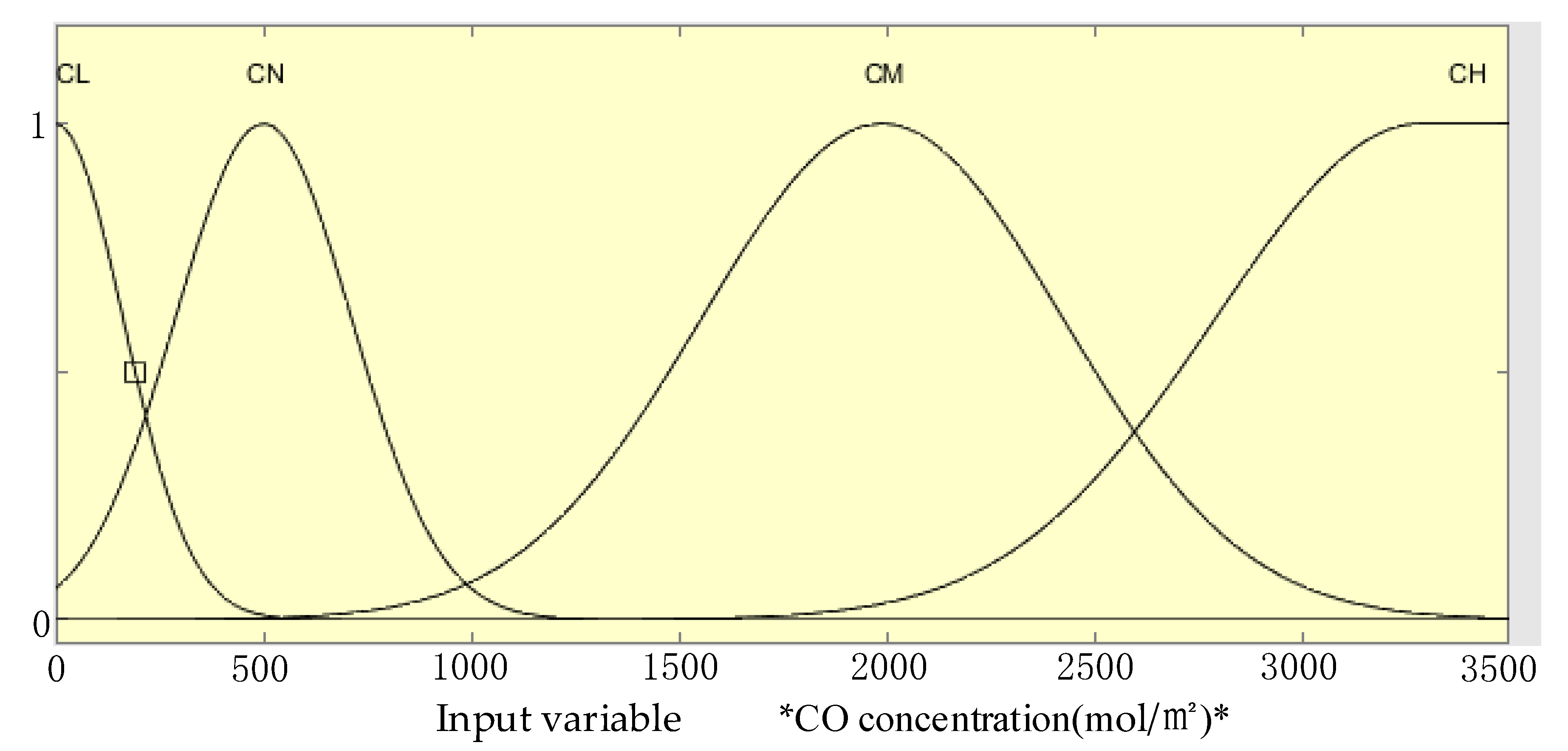
CO concentration is also an index that affects the detection of fire anomalies. Based on experience and expert analysis, it is determined that its domain is [0, 3500] and the unit is × 10⁻⁶ mol/mol. Divide it into four levels, which can be expressed as CO concentration є {CL,CN,CM,CH}, indicates that the CO concentration gradually increases. Its membership function is shown in Figure 11.

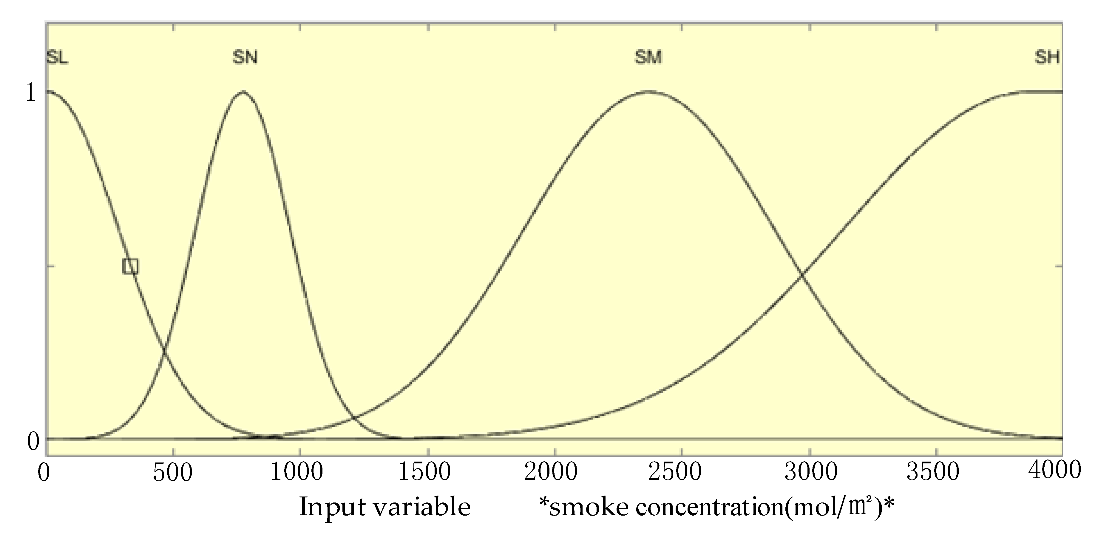
According to the literature search and expert experience analysis, the concentration of smoke is determined as [0, 4000], and the unit is × 10⁻⁶ mol/mol. Divide it into four levels, which can be expressed as smoke concentration є {SL,SN,SM,SH}, indicates that the smoke concentration gradually increases. Its membership function is shown in Figure 12:

4.4. Fuzzy Rule Establishment

Fuzzy rules are called linguistic rules or fuzzy “$If-Then$” rules, which is the language expression form of fuzzy inference rule. The general form is: If x is A Then y is B, A and B are fuzzy sets in the domain U and evaluation set V, respectively, and fuzzy rules are established based on the real-time fire risk assessment index system. Temperature, CO concentration, smoke concentration, personnel density are four inputs, and the security level is one output. The fuzzy rule form is expressed by the following formula: $Ifxis{A}_{i}andyis{B}_{i}andzis{C}_{i}andtis{D}_{i}Thenpis{W}_i$.

In the formula, x, y, z, and t are four input variables, which are output variables, are fuzzy sets, and are evaluation sets. Fuzzy rules are established by the risk evaluation index system and expert experience, as shown in

Table 2. Table of fuzzy rules.

Serial Number	Temperature	CO Concentration	Smoke Concentration	Security Level
1	TL	CL	SL	I
2	TN	CL	SL	II
3	TM	CL	SL	III
4	TH	CL	SL	IV
5	TL	CN	SL	II
6	TL	CM	SL	III
…	…	…	…	…
254	TH	CM	SN	III
255	TH	CM	SM	IV
256	TH	CH	SH	IV

.

4.5. Fuzzy Neural Network Training and Inspection

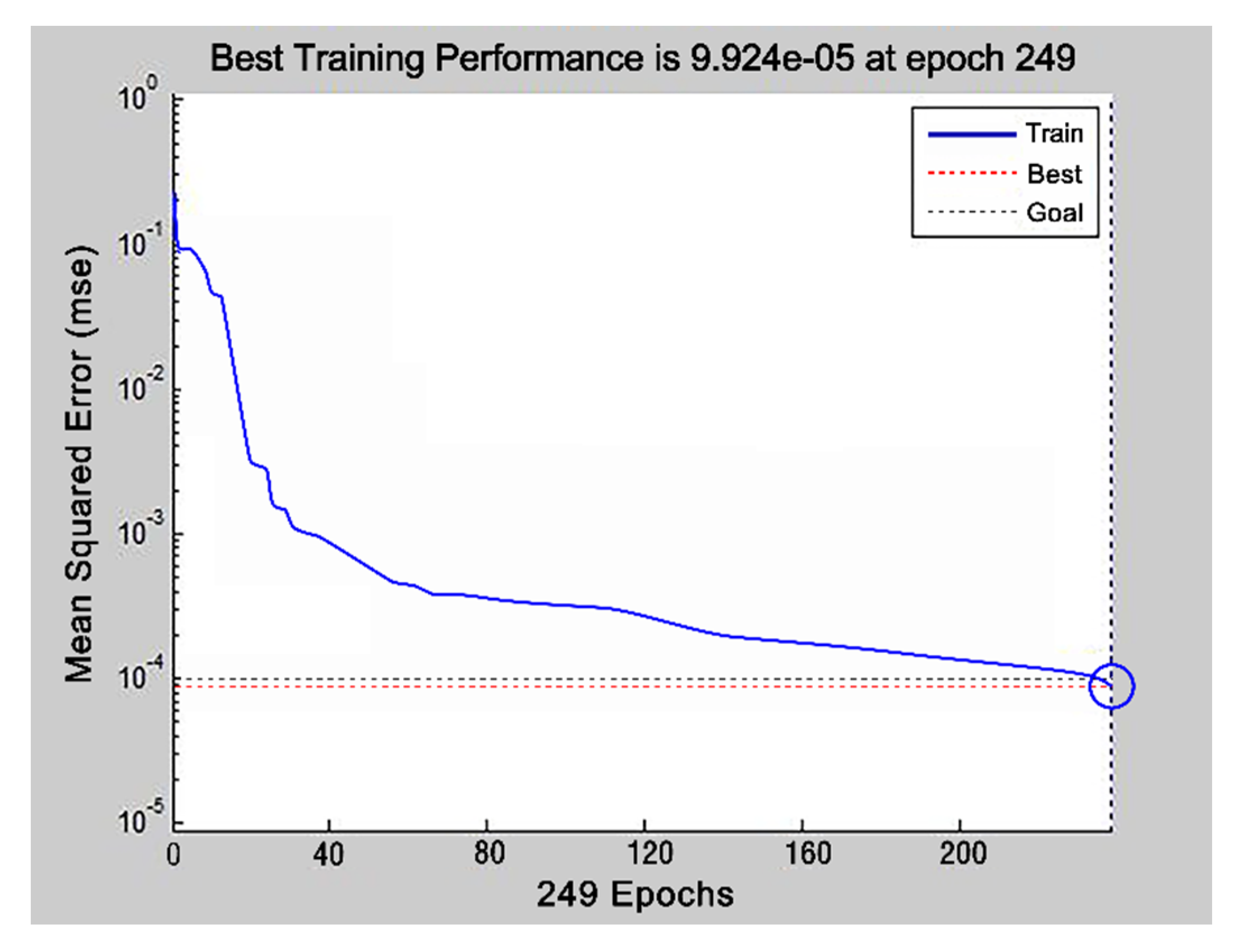
This training uses MATLAB software for simulation testing. In the network model, the training error is set to 0.0001, and the maximum number of trainings is set to 500 times. Figure 13 shows the mean square error graph after training. It can be seen that after 249 iterations, the training error is 9924 × 10–5, which meets the training setting requirements.

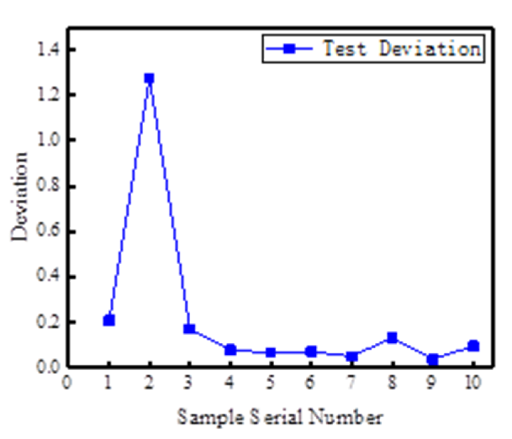
In order to verify whether the trained network model can accurately judge the risk assessment of the comprehensive fire situation, 10 groups of test samples were selected for testing, as shown in

Table 3. Test sample data and test results

Serial Number	Temperature (°C)	CO Concentration (× 10−6 mol/mol)	Smoke Concentration (× 106 mol/mol)	Expected Output	Actual Output
1	29.3	124.5	289.4	(1,0,0,0)	(0.83,0.13,0.08,0.01)
2	45.2	262.8	534.4	(0,1,0,0)	(0.04,0.17,0.87,0.09)
3	37.6	173.6	386.4	(1,0,0,0)	(0.91,0.09,0.04,0.01)
4	53.4	470.3	975.1	(0,1,0,0)	(0.04,0.93,0.03,0.01)
5	92.6	1134.2	2379.3	(0,0,1,0)	(0,0.02,0.95,0.04)
6	85.1	1023.4	2012.5	(0,0,1,0)	(0.01,0.03,0.94,0.03)
7	126.4	2124.4	4843.5	(0,0,0,1)	(0,0.02,0.04,0.96)
8	65.4	684.2	1462.7	(0,0,1,0)	(0.02,0.06,0.89,0.05)
9	78.4	873.1	1863.1	(0,0,1,0)	(0,0.02,0.97,0.12)
10	48.2	297.5	634.2	(0,1,0,0)	(0.14,0.92,0.08,0)

.

According to the test results in Table 3, the actual output of the network model is basically the same as the expected output. In order to more intuitively describe the pros and cons of the model’s performance, the error index $\gamma$ is used to describe the evaluation effect. The smaller the $\gamma$ is, the better the evaluation effect is. Calculation formula of error evaluation index:

$$\gamma =\left|y\left(n\right)-\widehat{y}\left(n\right)\right|$$

(17)

In the formula: $y\left(n\right)$ and $\widehat{y}\left(n\right)$ are the actual output value and expected output value of the network, respectively.

It can be seen from Figure 14 that the absolute error of the evaluation results of the fuzzy neural network model in this paper mostly fluctuates between 0.05 and 0.22, which proves that the fuzzy neural network model has high accuracy. It is feasible to use this method for comprehensive real-time situation risk assessment of fire.

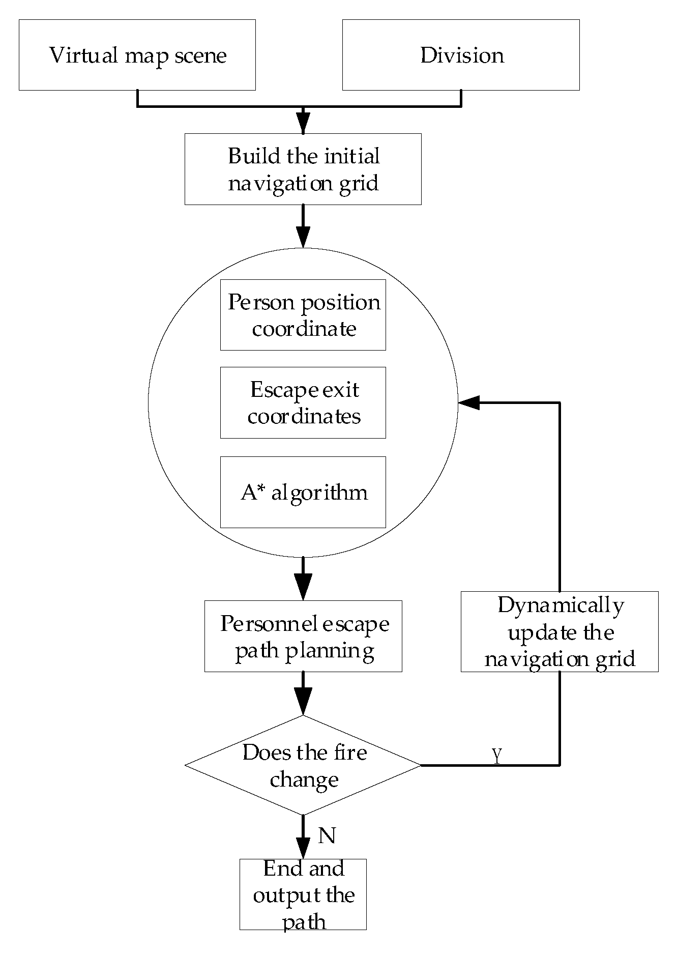
5. Escape Path Dynamic Planning Method

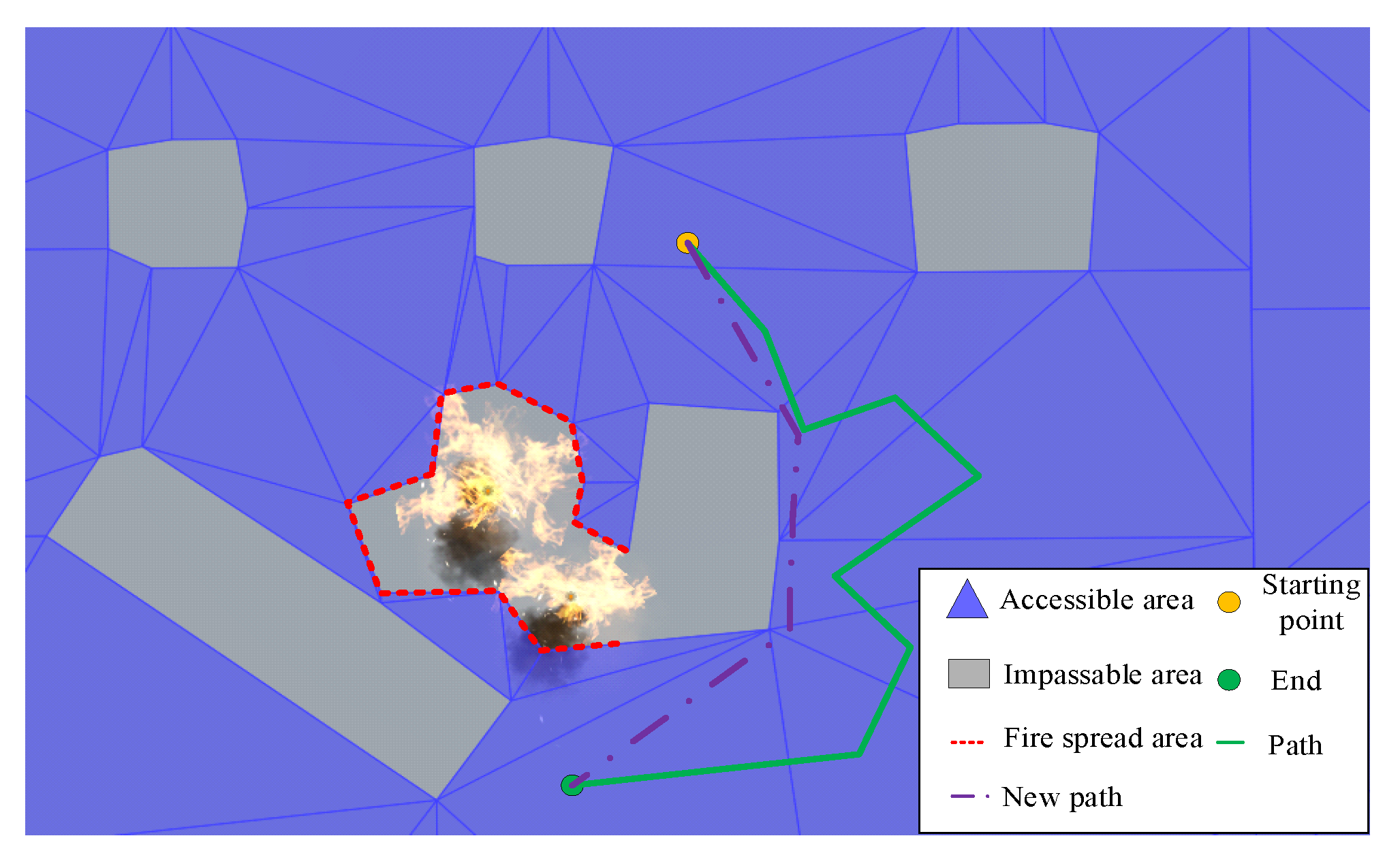
Figure 15 is a schematic diagram of the dynamic planning of the escape path:

The biggest advantage of this method is the real-time nature of path planning, Due to the complex structure in the cabin, including obstacles such as tables, chairs, doors, windows, electrical equipment, etc., in the event of a fire, the static environment of the cabin needs to incorporate the dynamic evolution of the fire information. The navigation grid can be updated in real time during the process of fire changes, and a new escape route can be obtained in real time with the path planning algorithm.

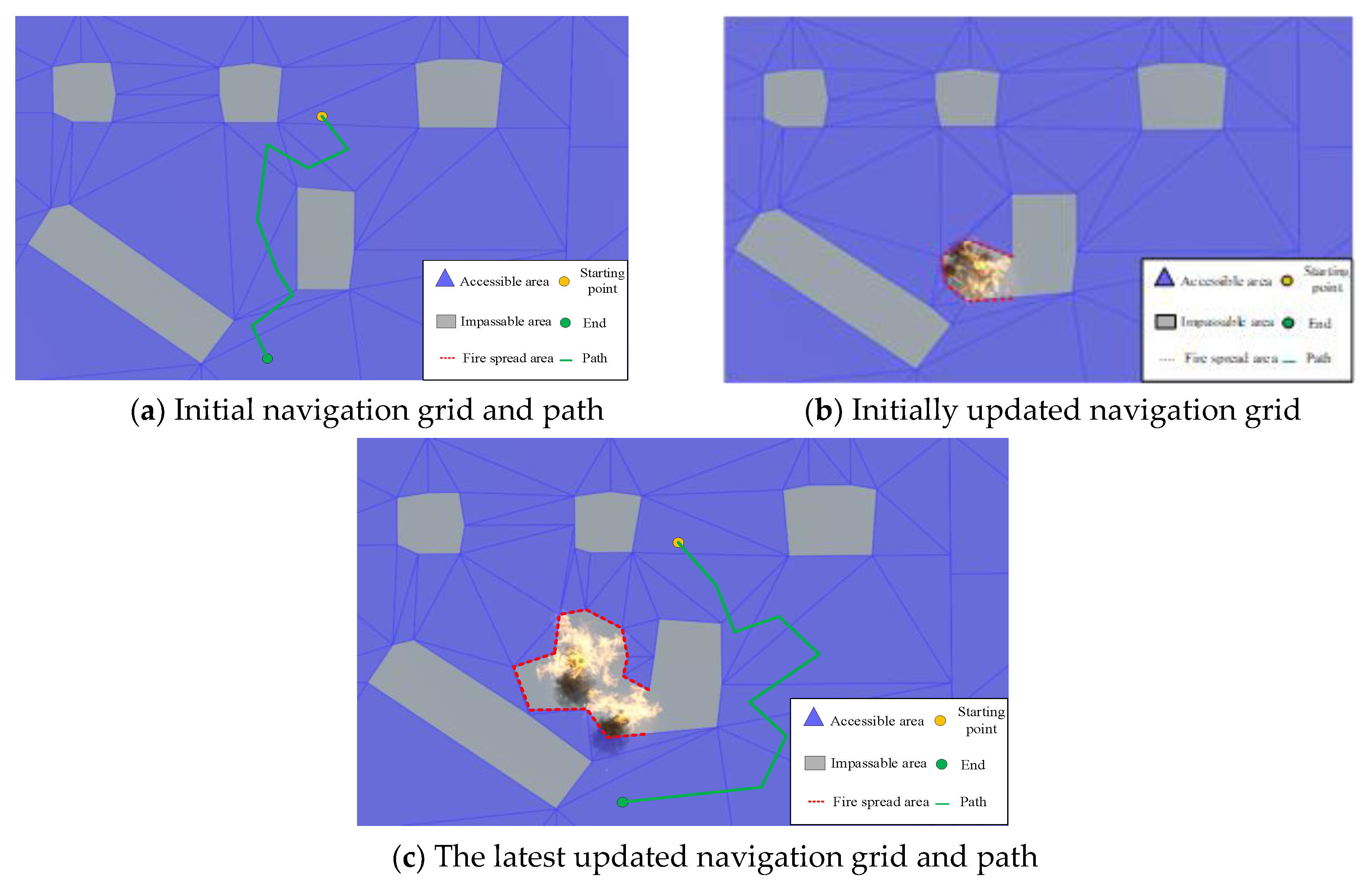
Figure 13 is a schematic diagram of the realization of the above path planning.

Figure 16a is the initial navigation grid and path generation diagram, the blue is the passable area, is the navigation grid generated by the triangulation method, the gray is the obstacle, the impassable area, the yellow solid point is the starting point, and the green. The solid point is the end point, and the green is the navigation path. Figure 16b is a schematic diagram of updating the navigation grid based on the spread of fire. It can be seen in the figure that when a fire occurs at a certain time, the surrounding temperature and CO concentration increase, and there is no condition for people to pass through. According to the temperature and CO concentration threshold set by the system, the excess position is regarded as an obstacle. The area enclosed by the solid red line in the figure is the fire spreading area, and the navigation grid is updated to the impassable area. The navigation grid is continuously updated as the fire spreading trend changes. As shown in Figure 16c, at a certain time after the fire, the area surrounded by the solid red line in the figure gradually expands, and the navigation grid continues to update. At this time, it can be found that the original path has been blocked by the spreading fire, and the route needs to be re-planned. The green implementation in the figure is the updated planned path.

It can be seen from the navigation path of the solid green line in Figure 16c that the actual length of the path is very long, the distance between the middle part and the impassable area is large, and it exceeds the walking radius of the person. It can be proved that this path has redundancy and cannot meet the shorter path length requirement. The selection of path nodes in the traditional A* path planning algorithm is to select the center of gravity of the triangulated grid, so the length of the generated path is not the shortest path, and the path node selection in the algorithm needs to be improved.

6. Improvement of A* Algorithm Based on Path Selection Node Selection

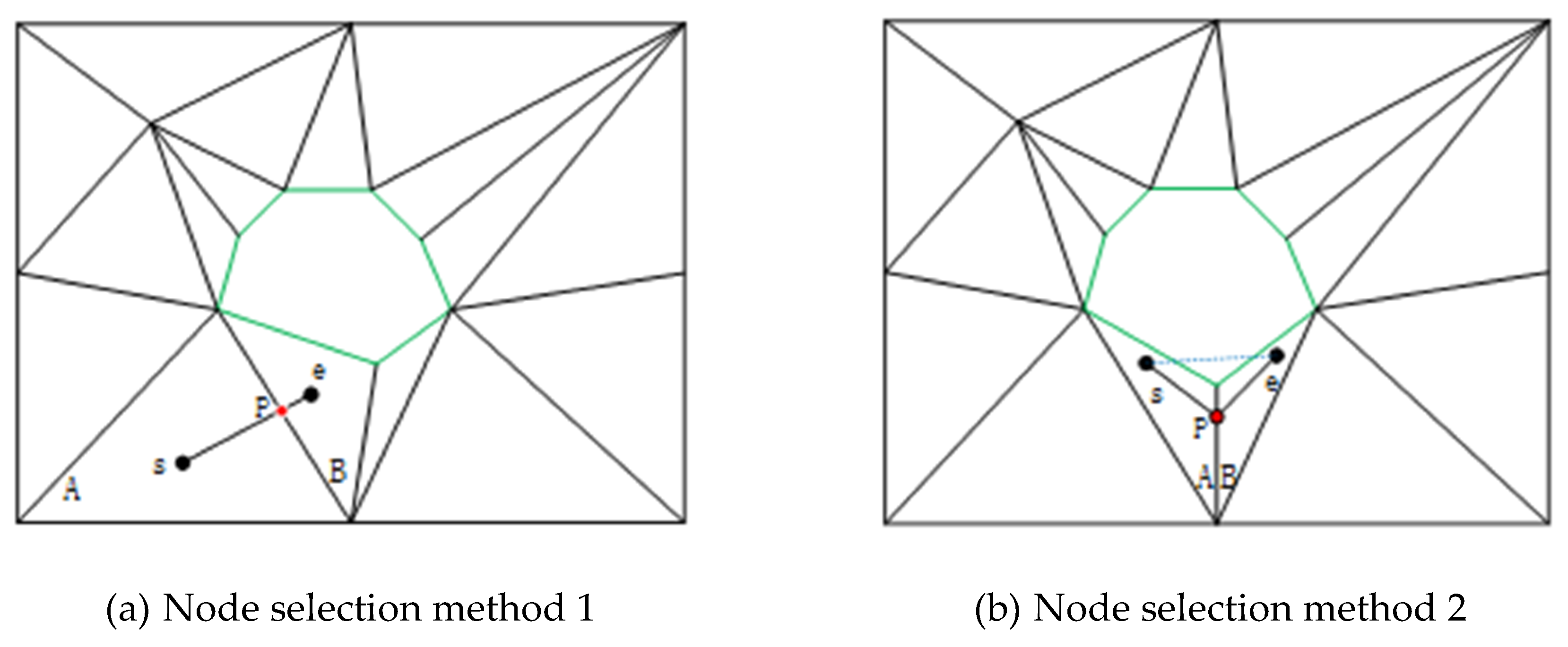
6.1. Choice of Wayfinding Nodes

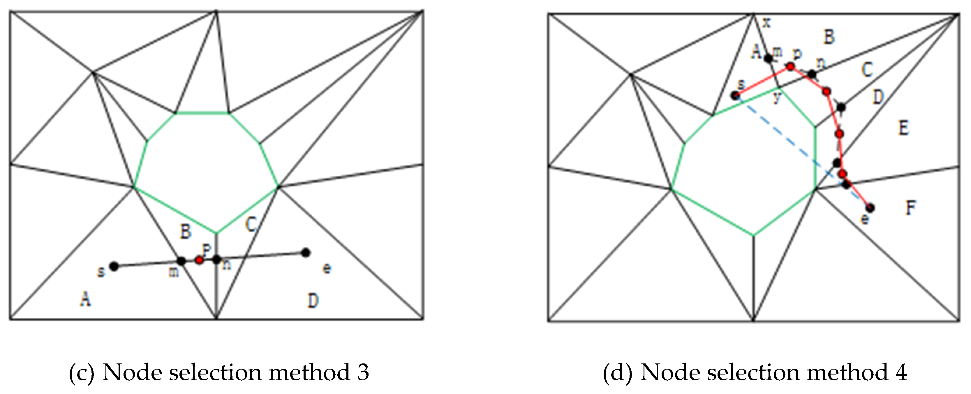
In view of the problems existing in the selection of navigation grid nodes, it is proposed that when selecting path nodes, while considering the shape of the grid, it is also necessary to consider the actual environmental conditions. Considering the environmental constraint edges, the choice of nodes is determined according to the positions of the starting point and the ending point. The following examples illustrate the selection of nodes in different situations:

Assuming that the starting point of the path is s, the ending point is e, A and B are triangular meshes, now looking for a path between points s and e. As shown in Figure 17a, the green boundary is the obstacle constraining edge, the starting point s is located in the triangular mesh A, and the ending point e is in the triangular mesh B. Moreover, se is the selection path, se line segment does not pass through the constraint edge, se line segment and triangle grid A, B red intersection point p, point e is the node of triangle grid B.

As shown in Figure 17b, the difference from (a) is that the position of the constraining edge and the shape of the A and B triangle meshes are different. The starting point s and the ending point e are respectively in the triangle grids A and B. At this time, the line segment se intersects with the green constraint edge. The grids A and B are adjacent. Select e as the node. However, at this time, it is necessary to select the point p as the path inflection point on the common edge, s-p-e as the path, and not to pass through the constraint edge.

As shown in Figure 17c, the starting point s and the ending point e are, respectively, in the triangular grids A and D, and the grids A and B are adjacent. At this time, the line segment se and A, B share the intersection of the point m. However, the entire line segment se does not have an intersection with the green constraint edge, so at this time the line segment se can still be used as a path, point s as a node in A, and e as a node in D. Take the midpoint p of the line segment mn as the node in B. The node in the grid C is the same as B. Then the connection between the nodes is the path.

As shown in Figure 17d, the triangular meshes A, B, C, D, E, and F are adjacent, the starting point s is in A, and e is in E, and the line segment se intersects the constraining edge, without passing through the triangular mesh grid. At this time, the nodes in the grid B cannot be obtained with simple line se intersection points. First, select two vertices x, y on the shared edge of A and B, and then use the Euclidean distance to calculate the value of line segment sx + xe and line segment sy + ye, namely $\left|sx\right|+\left|xe\right|$ and $\left|sy\right|+\left|ye\right|$. Similarly, the point n on the common edge of the adjacent triangle grids B and C is calculated, and then the point p in the line segment mn is calculated, which is the node in the triangle grid B. Use the same method to find the nodes in the triangular grids C, D, and E, and then connect each node to the starting point s and the ending point e, as shown by the red line in the figure, which is the final path.

6.2. A* Algorithm after Improved Node Selection Method

The traditional A* algorithm’s pathfinding method is improved so that it can adapt to different path node selection methods and search for the final optimal path. The traditional A* algorithm is a heuristic path search algorithm. The core is an evaluation function. This function estimates the cost of the node coordinates of the starting position to reach the current node and reach the predetermined target point from the current node, so as to achieve the purpose of path planning. The traditional estimation function is:

$$F\left(n\right)=G\left(n\right)+H\left(n\right)$$

where n is the location information of the current node. The evaluation function $F\left(n\right)$ can estimate the cost of the intermediate node n to the final target node; $G\left(n\right)$ represents the cost substitute value of the starting node to the current node n. $H\left(n\right)$ is a heuristic function, which is the core of the algorithm, and represents the cost generation value of the current node n reaching the target node. Heuristic function is used to estimate each point that is about to arrive, find the node with the smallest estimated value, and reach the target node to complete the search.

As shown in Figure 18, the A* algorithm flow chart after improving the node selection method.

In the flowchart, s and e are the starting node and the target node, T represents the triangular grid in the navigation grid, T.node represents the path node in the triangular grid. T, $G_{(s}{}_{,T)}$ is the actual distance value from the starting node to the triangle mesh node. $F=G_{(s}{}_{,T)}+H_{(T}{}_{,e)}$, $H_{(T}{}_{,e)}$ represents the Euclidean distance from the node of the current grid T to the target node e.OpenList1 is a set of triangles. T.AddOpen indicates whether T is added to the OpenList1 list, $OpenList1.Add\left(T\right)$ means add triangle mesh T to OpenList1 list, $OpenList1.Update\left(T\right)$ means update the triangle grid information in the list, $OpenList1.Remove\left(T\right)$ means delete the triangular grid T in the OpenList1 list. T.Closed indicates whether the triangle adjacent to the triangle mesh T has been visited, T.parent represents the triangular grid where the parent node of the triangular grid T is located, $OpenList1.Count$ represents the number of elements in the OpenList1 list.

The steps of the improved path search process of the node selection method are summarized as follows:

(1)

first, locate the starting node s and the target node e in the triangular grid set Ti. Get the starting triangle mesh Ts, the node of Ts is $T_s.node=s$, Go to step (2);

(2)

determine whether the target node e is in the triangular grid T. If it is False, go to step (3), if it is True, the pathfinding ends;

(3)

calculate the evaluation function F of the starting node Ts. At this time $G_{(s}{}_{,T)}$ is 0, $H=H_{(T}{}_{,e)}$, so $T_s.g=G_{(s}{}_{,T)},F_s=T_s.g+H_{(T}{}_{,e)}$. Add the triangle mesh Ts to the OpenList1 list. Go to step (2);

(4)

if the OpenList1 list is not empty, go to step (5); otherwise, it means that the path does not exist and end the search;

(5)

find the triangle mesh T1 with the smallest F value in the OpenList1 list, use this triangle mesh T1 as the current triangle, and then judge whether the nodes in it are equal to the target nodes. If it is True, then output the path, go to step (10), if it is False, go to step (6);

(6)

get the triangle grid T2 of T.Closed = False. Using the node selection method in Section (1), find the node n in T2 as the current node, if $T_2.AddOpen=True$ go to step (8), otherwise go to step (7);

(7)

if $T_2.AddOpen=False$, it is necessary to add T2 to the OpenList1list, $T_2.node=n$, $T_2.g=T_1.g+H_{(T1.node}{}_{,n)}$, $F_2=T_2.g+H_{(n}{}_{,e)}$. At the same time, save the triangle T1 where the parent node of T2 is located, $T_2.parent=T_1$, and go to step (9);

(8)

if T2 already exists in the OpenList1 list, compare the original F2 with the new F2′ value, $F_2{}^{’}=T_2{}^{’}.g+H_{(n}{}_{,e)}$, $T_2{}^{’}.g=T_1.g+H_{(T1.node}{}_{,n)}$, if F_2′< F₂, then T₂ = T_2′, F₂ = F_2′, $T_2.node=n$. Otherwise, do nothing and go to step (9);

(9)

if all adjacent triangle meshes of the current triangle mesh T1 are accessed, then $T_1.Closed=True$, then $OpenList1.Remove\left(T_1\right)$, go to step (4). Otherwise, do nothing and go to step (6);

(10)

through the traceback found in the parent attribute stored in the whole process, trace back from the target node e to the start node s, generate a path, and complete the pathfinding.

Figure 19 shows the pathfinding result of the improved A* algorithm. The pink dotted line path is the new path. Compared with the original green path, the path length is significantly shorter; thus, saving the escape time.

6.3. Optimize OPEN List Based on Binary Fork Method

From the principle of the A* pathfinding algorithm, it is known that maintaining the OpenList of nodes to be investigated is the key. Its main job is to compare and insert data into the delete operation. The insert operation is to insert the adjacent nodes of the current node into the OpenList list, sort and delete the node with the smallest F(n) from the list, and put it into the ClosedList. If the pathfinding map is large and the number of pathfinding nodes increases, then every time all nodes are compared, a bubble sorting method is performed. The time overhead of traversing once is very large, resulting in reduced efficiency.

This paper uses the binary fork data structure to store the OpenList list. The principle of the binary fork is similar to the binary tree, which satisfies the characteristics of the heap. It is a complete binary tree stored in order of size. Divided into two types of minimum and maximum binary stack—the characteristic of the minimum binary fork is that the value of the parent node is less than or equal to the value of any child node, and the characteristic of the binary fork is that the value of the parent node is greater than or equal to the value of any child node. According to the characteristics of selecting the node with the smallest F(n) in the OpenList list, the smallest binary heap is selected to store the node in the OpenList list.

As shown in Figure 20, is a binary heap storage data structure diagram, the value in each circle represents the node F(n), the circle at the top of the heap represents the smallest F(n). Each time the pathfinding process is performed, the OpenList list is updated, the left and right nodes are added, and the useless nodes in the list are deleted.

Inserting data into the binary fork only requires creating a hole in the available location, without destroying the data structure. If it does not conform to the data order, continue to insert upwards until it is correctly inserted. To delete data, you only need to delete the position of the root node, and then assign a value to adjust from top to bottom until the heap order is satisfied. The use of binary heap storage OpenList column can quickly insert and delete data node operations, improve the efficiency of the A* pathfinding algorithm.

6.4. Improvement of Heuristic Function of A* Algorithm

In a complex three-dimensional environment with a fire in the cabin, the elevator is undesirable in the case of multiple floors. Most of the escapes depend on stairs, and the stairs are mapped to the virtual environment map representation. It is urgent to consider the height and slope of the plane.

Some attributes are specified in the design of the cabin, which limits the walking area of the pathfinding object. It has a certain ability to read obstacles and climbing ability. Climbing can be understood as the ability to take stairs. In the original A* algorithm evaluation function, the calculation of the G value and the H value is a simple distance calculation between two points, using the Euclidean distance, but due to the actual pathfinding environment requirements, the $G\left(n\right)$ and $H\left(n\right)$ functions in the $F\left(n\right)$ calculation need to be improved. Obtain the normal vector of a plane from the three-dimensional scene; the plane tilt angle is expressed by the cosine of the angle, as shown in formula (18). Vector ${\overrightarrow{n}}_1$ is the normal vector of the walking hierarchical plane, ${\overrightarrow{n}}_0$ is the normal vector of the ground, and ${\theta }_p$ is the angle of inclination formed by the plane and the ground.

$$\cos {\theta }_p=\frac{\overrightarrow{n_1}\cdot \overrightarrow{n_0}}{\overrightarrow{\left|n_1\right|}\times \left|\overrightarrow{n_0}\right|}$$

(18)

$G\left(n\right)$ function improvement: define function $G\left(V_s,V_0\right)$ as the actual distance from the starting node $V_s$ to the current node $V_0$, as shown in formula (19):

$$G\left(V_s,V_o\right)={\displaystyle \sum _{p=s}^{n-1}\left(d\left(V_p,V_{p+1}\right)\times \left(2-\cos \left(\frac{\pi }{2\alpha }\times {\theta }_{p+1}\right)\right)\right)}$$

(19)

In the formula: $d\left(V_p,V_{p+1}\right)$ is the Euclidean distance between nodes $V_p$ and $V_{p+1}$; $\alpha$ is the maximum slope that can be crossed, and ${\theta }_{p+1}$ is the slope of the plane where node $V_{p+1}$ is located. If the value of $\alpha$ is between 0 and π/2, the range of cost consumption between the two points is between $d\left(V_p,V_{p+1}\right)$ and $2d\left(V_p,V_{p+1}\right)$. When ${\theta }_{p+1}=\alpha$, the cost consumption value between two points is $2d\left(V_p,V_{p+1}\right)$.

Improvement of function $H\left(n\right)$: define function $H\left(V_0,V_e\right)$ as the estimated distance from the current node $V_0$ to the target node $V_e$, as shown in formula (20).

$$H\left(V_0,V_e\right)=\left|V_{ey}-V_{oy}\right|+\sqrt{{\left|V_{ex}-V_{ox}\right|}^2+{\left|V_{ey}-V_{oy}\right|}^2+{\left|V_{ez}-V_{oz}\right|}^2}$$

(20)

where $\left|V_{ey}-V_{oy}\right|$ is the distance difference between the current node and the target node in the y direction, $\sqrt{{\left|V_{ex}-V_{ox}\right|}^2+{\left|V_{ey}-V_{oy}\right|}^2+{\left|V_{ez}-V_{oz}\right|}^2}$ represents the Euclidean distance between the current node and the target node. Since it is a three-dimensional scene, the $H\left(n\right)$ function needs to consider height information.

The improved estimation function is shown in Formula (21):

$$F\left(n\right)=G\left(V_s,V_o\right)+H\left(V_0,V_e\right)$$

(21)

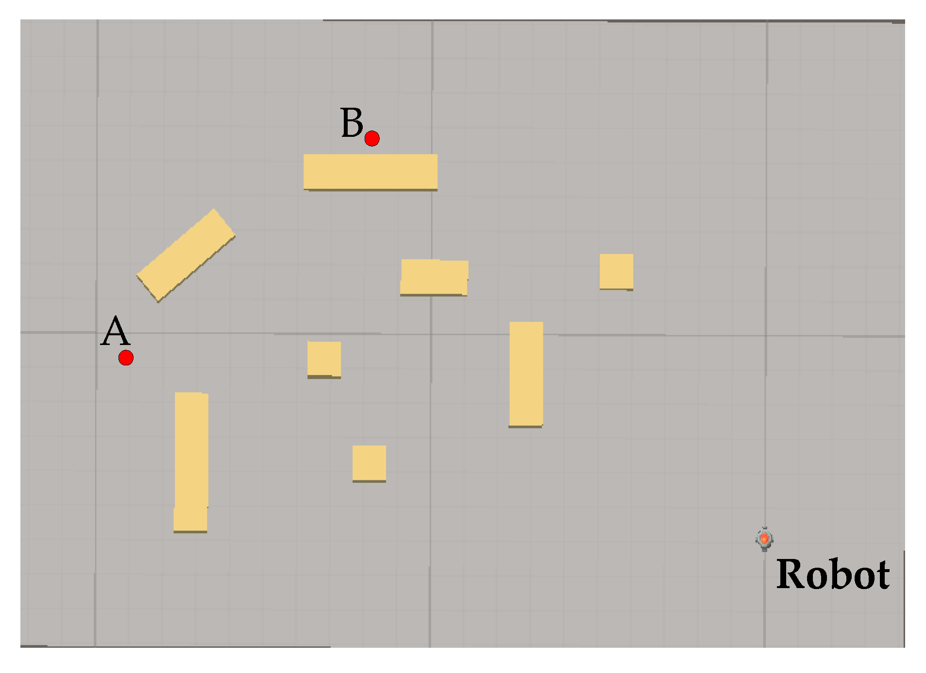
6.5. Path Planning Simulation Experiment

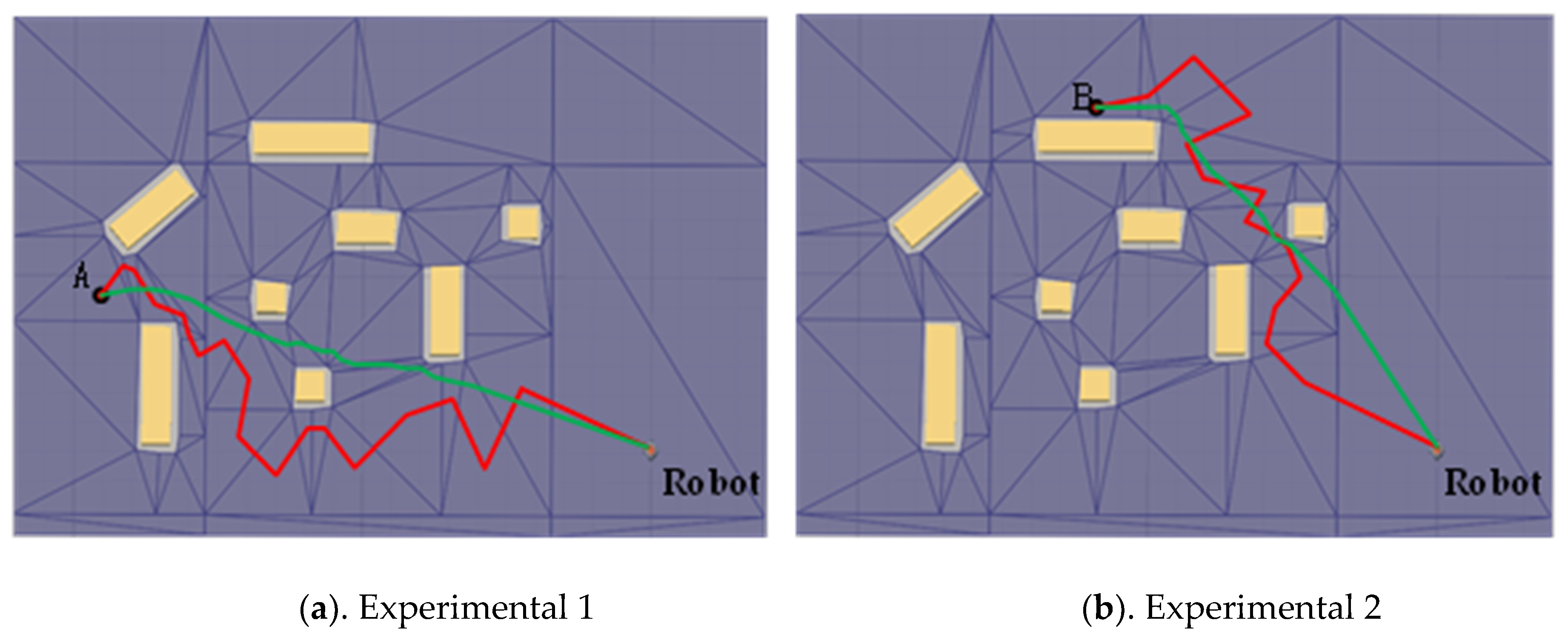
In order to verify the performance of the improved A* algorithm, comparing the traditional A* algorithm and the improved A* algorithm in the path planning experiment on the same plane. Build the experimental model shown in Figure 21, including obstacles, path-finding robot, A and B two target points.

Figure 22a,b are the results of the two experimental path planning. The starting point A and the target point B of the two experiments are located at different positions. The paths generated by the traditional A* algorithm and the improved A* algorithm are represented by red and green curves respectively.

In order to analyze the difference between the two algorithms more intuitively, the performance of the two algorithms is analyzed and compared from three aspects: the number of pathfinding nodes, pathfinding length, and pathfinding time. According to the data analysis in

Table 4. Performance comparison between traditional A* algorithm and improved A* algorithm.

Experiment Number	Traditional A* Algorithm			Improved A* Algorithm
	Number of Nodes	Path Length	Time/ms	Number of Nodes	Path Length	Time/ms
1	86	41	10.02	53	32	7.53
2	83	39	11.01	49	31	8.02

, the number of nodes searched by the improved A* algorithm is lower than that of the traditional A* algorithm, so the corresponding search time is reduced by 26.05% on average compared with the traditional algorithm, and the path planning length is reduced by 11.07% on average. It can be seen that compared with the traditional A* algorithm, the improved A* algorithm is improved in terms of path planning speed and path planning length and rationality.

7. Conclusions

This paper establishes a ship model and conducts simulation to determine the law of fire spread. Taking 63,500 DWT oil tanker cabin as the research object, the fire propagation characteristic object is analyzed, and the mathematical and physical models of ship fire simulation are constructed. The simulation calculation area and the setting of fire source information parameters and boundary conditions are determined, and three working condition parameters are set for simulate, and get experimental data.

According to the law of fire spread, establish a fire risk assessment system. Establish a comprehensive real-time fire risk assessment index system for complex and diverse fire environments with complex temperature, smoke concentration, CO concentration, and personnel density.

Establishing a Fire Spread Situation Risk Assessment Model Based on Fuzzy Neural Network. Use MATLAB software to establish an evaluation model based on fuzzy neural network to carry out fuzzy comprehensive quantitative analysis of the multi-element information in the cell grid. It is proved that the fuzzy neural network model has high accuracy, and it is feasible to use this method for comprehensive real-time fire risk assessment.

The principle and method of constructing the initial navigation grid are described. The initial cabin navigation grid is constructed, and a dynamic generation method of navigation grid (based on fire spread information), and a dynamic planning method of escape route (based on ship fire spread) are proposed.

Improve the traditional A* algorithm and conduct experimental verification. This paper improves the path node selection method, search process, node data storage method, and heuristic function in the traditional A* algorithm. The algorithm performance is compared through the path planning simulation experiment. The experimental results show that the path finding algorithm is suitable for three-dimensional path finding and the path planning time is 26.05% lower than the traditional algorithm, and the path length is 11.07% lower than the traditional algorithm. The path finding efficiency is better. This article only improves the A* algorithm for a single scenario. In the future, we can consider improving the A algorithm in more complex environments.

References

- Li, T. Simulation Study on Temperature and Smoke Law of ship’s Closed Cabin Fire Field. Master’s Thesis, South China University of Technology, Guangzhou, China, 2017. [Google Scholar]
- Xie, Q.; Zhang, S.; Wang, J. A surrogate-based optimization method for the issuance of passenger evacuation orders under ship fires. Ocean Eng. 2020, 209, 107456. [Google Scholar] [CrossRef]
- Peng, Y.; Li, S.; Hu, Z. A self-learning dynamic path planning method for evacuation in large public buildings based on neural networks. Neurocomputing 2019, 365, 71–85. [Google Scholar] [CrossRef]
- Chou, J.-S.; Cheng, M.-Y.; Hsieh, Y.-M.; Yang, I.-T.; Hsu, H.-T. Optimal path planning in real time for dynamic building fire rescue operations using wireless sensors and visual guidance. Autom. Constr. 2019, 99, 1–17. [Google Scholar] [CrossRef]
- D’Amore, G.K.O.; Marinò, A.; Kašpar, J. Numerical Modeling of Fire Resistance Test as a Tool to Design Lightweight Marine Fire Doors: A Preliminary Study. J. Mar. Sci. Eng. 2020, 8, 520. [Google Scholar] [CrossRef]
- Sun, Q.; Turkan, Y. A BIM-based simulation framework for fire safety management and investigation of the critical factors affecting human evacuation performance. Adv. Eng. Inform. 2020, 44, 101093. [Google Scholar] [CrossRef]
- EL Mostafa, B.; Abdelghani, C. Efficacy of Virtual Reality for Studying People’s Pre-evacuation Behavior under Fire. Int. J. Hum.—Comput. Stud. 2020, 142, 102484. [Google Scholar]
- Ryu, E.-G.; Yang, C.-S.; Choi, J.-W. Fundamental Research for Escape Guidance System Development of Passenger Ship. J. Korean Navig. Port Reserch 2017, 41, 39–46. [Google Scholar] [CrossRef] [Green Version]
- Wang, B.; Li, H.; Rezgui, Y.; Bradley, A.; Ong, H.N. BIM based virtual environment for fire emergency evacuation. Sci. World J. 2014, 2014, 589016–589022. [Google Scholar] [CrossRef]
- Xiong, Q.; Zhu, Q.; Du, Z.; Zhu, X.; Zhang, Y.; Niu, L.; Li, Y.; Zhou, Y. A dynamic indoor field model for emergency evacuation simulation. ISPRS Int. J. Geo-Inf. 2017, 6, 104. [Google Scholar] [CrossRef]
- Cui, L. Research on Intelligent Escape Navigation Technology for Indoor Fire. Master’s Thesis, East China University of Science and Technology, Shanghai, China, 2014. [Google Scholar]
- Chenghua, O.; Chaochun, L.; Siyuan, H.; Sheng, J.J.; Yuan, X. Fine reservoir structure modeling based upon 3D visualized stratigraphic correlation between horizontal wells: Methodology and its application. J. Geophys. Eng. 2017, 14, 1557–1571. [Google Scholar] [CrossRef] [Green Version]
- Wu, H.; Yang, J.; Chen, C.; Wan, Y.; Zhu, X. Research of Virtual Ship Fire-fighting Training System Based on Virtual Reality Technique. IOP Conf. Ser. Mater. Sci. Eng. 2019, 677, 042100. [Google Scholar] [CrossRef] [Green Version]
- Wang, R.; Li, D.; Miao, K. Optimized Radial Basis Function Neural Network Based Intelligent Control Algorithm of Unmanned Surface Vehicles. J. Mar. Sci. Eng. 2020, 8, 210. [Google Scholar] [CrossRef] [Green Version]
- Cheng, Z.; Xu, Y.; Zhu, Q. Research and simulation of fire escape route algorithm based on fuzzy theory. J. Beijing Univ. Chem. Technol. 2016, 43, 115–122. [Google Scholar]
- Guo, L.; Shi, W.; Li, Y.; Li, F. Adaptive grid map creation algorithm based on quadtree. Control Decis. 2011, 26, 1690–1694. [Google Scholar]
- Ahn, S.; Doh, N.L.; Lee, K.; Chung, W.K. Incremental and robust construction of Generalized Voronoi Graph (GVG) for mobile guide robot. In Proceedings of the Proceedings 2003 IEEE/RSJ International Conference on Intelligent Robots and Systems (IROS 2003) (Cat. No.03CH37453), Las Vegas, NV, USA, 27–31 October 2003. [Google Scholar]
- Xu, S.; Cao, Q. Mobile robot path planning based on visual view. Comput. Appl. Softw. 2011, 28, 220–222, 236. [Google Scholar]
- Li, P.; Zhu, J.; Peng, F.; Yang, L. Path planning based on visual view and A* algorithm. Comput. Eng. 2014, 3, 193–195, 200. [Google Scholar]
- He, X. Research on Dynamic Path Planning of Characters in Interactive Virtual Scenes. Master’s Thesis, China University of Geosciences, Beijing, China, 2018. [Google Scholar]
- Wang, T.; Zhang, L. A route search technology based on navigation grid. Comput. Knowl. Technol. 2010, 6, 3014–3016. [Google Scholar]
- Zhu, C.; Liu, L. Improved A~* algorithm based on polygon navigation grid map. Softw. Guide 2019, 18, 17–21. [Google Scholar]
- Chen, S. Research on Map Game Pathfinding Based on Improved A~* Algorithm. Master’s Thesis, Chongqing Normal University, Chongqing, China, 2016. [Google Scholar]
- Wu, Y.; Yang, J. Robot path planning based on A~* algorithm. Electron. Sci. Technol. 2017, 30, 124–127. [Google Scholar]
- Jin, H.; Wang, Y.; Yuan, M.; Chen, M. Improved A~* high-rise building escape path planning algorithm. Bull. Surv. Mapp. 2019, 11, 17–21, 25. [Google Scholar]
- Tang, J.; Zhu, J.; Li, W.; She, P. Realistic visualization of indoor fire based on virtual geographic environment. Geogr. Inf. World 2019, 26, 72–76. [Google Scholar]
- Gu, F. Research and Application of Fuzzy Neural Network in Fire Detection in Shopping Malls. Master’s Thesis, Anhui University of Science and Technology, Anhui, China, 2019. [Google Scholar]
Figure 3.
Schematic diagram of measuring point layout.
Figure 4.
Detector layout.
Figure 5.
Temperature change curve.
Figure 6.
Smoke concentration curve.
Figure 7.
CO concentration curve.
Figure 8.
Comprehensive evaluation system.
Figure 9.
T-S Fuzzy neural network structure diagram.
Figure 10.
Graph of temperature membership function.
Figure 11.
The concentration of CO belongs to the graph of the function.
Figure 12.
The smoke concentration belongs to the function graph.
Figure 13.
Training error curve.
Figure 14.
The network model evaluates the absolute error graph.
Figure 15.
Dynamic navigation grid update process.
Figure 16.
Path planning based on dynamic update of navigation grid.
Figure 17.
Node selection algorithm diagram.
Figure 18.
Improvement Path-finding flow chain.
Figure 19.
Pathfinding result graph after improving A* algorithm.
Figure 20.
A binary heap stores data structures.
Figure 21.
Flat experiment environment.
Figure 22.
Experimental path planning results.