Buoyant Jets in Cross-Flows: Review, Developments, and Applications


Department of Civil Engineering, University of Ottawa, 75 Laurier Ave E, Ottawa, ON K1N 6N5, Canada
*
Author to whom correspondence should be addressed.
J. Mar. Sci. Eng. 2021, 9(1), 61; https://0-doi-org.brum.beds.ac.uk/10.3390/jmse9010061
Submission received: 11 November 2020
/
Revised: 5 January 2021
/
Accepted: 6 January 2021
/
Published: 8 January 2021
(This article belongs to the Special Issue Feature Reviews in Marine Science and Engineering)
Abstract
:Significant environmental effects from the use of marine outfall discharges have led to increased efforts by both regulatory bodies and research groups to minimize the negative impacts of discharges on the receiving water bodies. Understanding the characteristics of discharges under conditions representative of marine environments can enhance the management of discharges and mitigate the adverse impacts to marine biota. Thus, special attention should be given to ambient cross-flow effects on the mixing behaviors of jet discharges. A buoyant jet in cross-flow has different practical applications such as film cooling and dilution, and provide a higher mixing capability in comparison with free jets or discharges into stationary environments. The main reason for this is believed to be the existence of various complicated vortical structures including a counter-rotating vortex pair as the jet expands downstream. Although tremendous research efforts have been devoted to buoyant jets issuing into cross-flows over the past five decades, the mixing process of an effluent at the discharge point is not yet well understood because of the highly complex fluid interactions and dispersion patterns involved. Therefore, there is a need for a deeper understanding of buoyant jets in cross-flows in order to obtain better predictive methods and more accurate design guidelines. The main aims of this study were (i) to establish the background behind the subject of buoyant jets in cross-flows including the flow structures resulting from the interaction of jets and cross-flows and the impacts of current on mixing and transport behavior; (ii) to present a summary of relevant experimental and numerical research efforts; and finally, (iii) to identify and discuss research gaps and future research directions.
1. Introduction and Background
Currently, the worldwide growth of effluent discharges into receiving water bodies has become a critical concern as a consequence of industrialization and rapid population increase [1,2]. Effluent discharges can be either in the form of brine discharge as a by-product of desalination plants or in the form of thermal discharge, which corresponds to some industrial activities including thermal power plants and mining. The former has a wide range of applications typically in arid and semi-arid countries, while the latter has broad applications in countries such as Canada [2]. In most relevant engineering applications such as seawater desalination plants, the discharge is almost always as a turbulent buoyant jet (containing both buoyancy and momentum fluxes) [3,4]. This is caused by the difference between the density of the jet and the receiving water body due to differences in salinity, temperature, or chemical composition [4,5].
Regardless of type, these effluents can be harmful to the environments they are released into. Decreases in water quality, destruction of marine habitats, and damage to near-shore recreational sites represent some of the adverse impacts on the environment. Therefore, it is necessary to study effluent outfall characteristics and designs for the purpose of minimizing their environmental impacts while adhering to regulatory demands. In this situation, utilizing buoyant jets may be a practical remedy that is capable of improving the mixing and dispersion of effluent discharges in the receiving waters. Several experimental, analytical, and numerical studies have focused on the topic of the mixing of buoyant jets within the receiving water bodies (e.g., [4,6,7,8,9,10]).
The interaction of multiple factors relevant to the discharge and receiving water bodies determines the dilution, dispersion, and even biological impacts of effluent discharges. Generally, three main types of factors should be considered when evaluating the environmental risk of a discharge including [11]:
- (i)
- discharge characteristics (such as type of discharge structure and effluents);
- (ii)
- receiving environment characteristics (such as topography and other physical and biological characteristics); and
- (iii)
- forcing functions (such as currents and waves).
Regarding the interplay with ambient hydrodynamic forces, buoyant jets can be discharged into two main types of receiving water: stationary and dynamic environments. Discharges into stationary environments, which is the usual basis for the design of turbulent buoyant jets as well as the worst case in terms of mixing and dilution [2], have been the main focus of previous studies since the 1970s. Several improvements have been obtained for this type of discharge over the last few decades. For example, in the literature [8,12,13,14,15,16,17,18,19,20,21], a general agreement has been noted for the optimal design of effluent discharges, with inclined jets yielding greater mixing and dilution than vertical ones. Particularly with the selection of a 60° inclination angle, it is generally believed that the highest dilution may be achieved at the return point, with a few exceptions.
However, the oceanic receiving environment is rarely stationary, and the impact of an ambient cross-flow on the mixing process of effluent discharges at the discharge point should be well comprehended because of the highly complex fluid interactions and dispersion patterns involved [22]. Investigations have shown that the flowing current influence mainly results in the extension of the jet trajectory as well as the enhancement of jet-mixing [23,24,25,26].
Basically, the jet in cross-flow (JICF) or transverse jet is related to a jet of fluid being ejected from a nozzle and interacting with the ambient fluid flowing across the nozzle exit [27,28], with both the jet and the cross-flow being changed after their interaction [29]. The flow characteristics of the cross-flow after being hindered by the jet can be interpreted similarly to those of a flow around a circular cylinder. In addition, due to the influence of the cross-flow, the jet gets deflected, and an energy and momentum exchange between the jet and the boundary shear-layer zone of the cross-flow takes place [27]. Highly complex three-dimensional, unsteady, and nonlinear flows are generated because of the interaction between the cross-flow and the jet [22]. As a result, the understanding and control of JICFs are of significant interest.
JICFs have a wide variety of practical applications including plume dispersion, film cooling for combustors and turbines, and discharges of sewage and industrial effluents into channels and natural rivers [22,27,30]. JICFs have also gained considerable attention in many experimental and numerical studies in fluid mechanics due to their capability to provide higher mixing in comparison with free jets [22,31]. This is mostly attributed to the existence of various complicated vortical structures resulting from the interaction of the jet and cross-flow as the jet expands downstream [28,30,32]. It should be noted that most of the previous studies on the formation and evolution of vortical structures have involved using buoyant JICF applications involving film cooling. Thus, using this knowledge can also help in understanding the impacts of vortical structures on mixing behaviors in dilution applications.
Fifty years of JICF research was explored in a study by Margason [33], and several more achievements have been made in this field since then. Although significant research efforts have recently been devoted to buoyant jets issuing into cross-flows, a deficiency in comprehension of their discharge behavior in dynamic receiving environments still remains [34].
A review of buoyant JICFs is thus helpful in providing general principles and better knowledge in order to improve the understanding of the mixing behavior of buoyant jets and their performance under more realistic oceanic conditions (i.e., dynamic environments). Generally, two main focuses have drawn the attention of researchers in the study of buoyant JICFs including the flow structures due to the interaction of jets and cross-flows and the effects of flowing currents on the mixing and transport behavior in near- and far-field regions. In order to protect the receiving water bodies and enhance the management of discharges, such information is of significant importance. Thus, the objectives of this review study were (i) to understand buoyant JICF flow structures and mixing and transport behaviors; (ii) identify the critical issues obtained from the experimental and numerical fields for these flow structures and mixing and transport behaviors; and (iii) highlight a range of knowledge gaps regarding future research directions.
The rest of this paper is organized as follows. Section 2 presents the most practical engineering applications introduced for buoyant JICFs and some of the influencing factors that should be considered in their design. Theoretical analysis, experimental techniques, and numerical modeling, which are the applicable assessment approaches to investigate the interactions of buoyant jets and cross-flows, are reviewed in Section 3, Section 4 and Section 5, respectively. In Section 6, the existence of different vortical structures as significant structures that can be formed and evolved in the flow field of buoyant JICFs are discussed. Then, the entrainment and mixing mechanisms involved in buoyant JICFs are explained in Section 7. Section 8 deals with the experimental and numerical research efforts on understanding the flow structures and mixing behaviors of buoyant JICFs. Finally, a summary of relevant research gaps and concluding remarks are identified and presented in Section 9 and Section 10, respectively.
2. Engineering Applications of Buoyant Jet in Cross-Flow (JICF)
There are many essential engineering applications introduced for buoyant JICFs such as film cooling of gas turbine blades, fuel atomization in scramjets, and applications involving dilution [27]. According to the main goal expected, various jet penetration levels are needed, which can be achieved by the changes in the ratios of jet to cross-flow velocity (; is the jet discharge velocity and is the ambient flow velocity) and jet to cross-flow momentum flux (; is the jet discharge density and is the ambient flow density) [30,35]. For instance, the jet penetration levels and molecular mixing of the jet with its surrounding field are expected to be high for applications involving dilution, since the momentum flux ratio often exceeds 25 or even J > 100 [30]. However, the momentum flux ratio is relatively low (often J < 5 or J < 1) for film cooling applications in order to be able to thermally protect turbine blades [30]. In addition, when it comes to the engineering design of buoyant JICFs, the velocity ratio can be introduced as an important aspect of lateral jet-flow structures [27].
In the following sections, an introduction to two of the most practical engineering applications of buoyant JICFs, namely film cooling and brine water dilution, will be briefly presented.
2.1. Film Cooling
In film cooling applied in gas turbines, the coolant jet is injected into the hot cross-flow while requiring to be attached to the wall. The coolant then generates a thin layer over the turbine blades, which protects the surface from direct exposure to the hot cross-flow [27]. Additionally, the cooling medium interacts with the main stream to eliminate some of the heat [36]. The Reynolds number, velocity ratio, turbulence, hole geometry, inclination angle, and density ratio are among the effective parameters while studying the film cooling performance. Consequently, studies on this application should be shifted from uni-variate to multi-variate assessments. Mechanisms of the JICF’s vortical structure formation should also be considered in order to get closer to the realistic working conditions [27].
2.2. Dilution
Brackish water discharges (as dense jets) into a flowing water body emitted by osmotic power plants have remarkable environmental impacts and undergo complex mixing processes [4,37]. Accordingly, a deep knowledge of the interaction between the discharge system and the receiving body is required to investigate the mixing process as well as the potential environmental effects. A definition schematic of a dense jet discharge into a receiving water body and the relevant key dimensional properties are given in Figure 1. The dense jet discharges an effluent with a density of and a velocity of U0 through a round nozzle with a diameter of D, an angle relative to the horizontal of , and a port height of z0 into the receiving environment with a depth of H, a fluid density of , and a uniform ambient flow velocity of Ua.
According to the literature [4,12,37,38,39], the behavior of a dense jet issuing into a cross-flow can generally be classified into two phases: the rapid ascent and gradual descent phases. Apart from the influence of the cross-flow, the jet’s movement is governed by the interplay of discharge buoyancy and momentum forces [40]. As the jet rises, the negative impact of buoyancy forces on the jet’s vertical penetration leads to a reduction in its momentum before it begins to sink. The jet peaks its maximum terminal height (ztm) and its maximum centerline height (zt) at a downstream distance of xt with a centerline peak dilution of St. Then, the jet gradually falls during the descent phase due to the downward buoyancy forces until impacting at distance xi with dilution Si. A laterally bottom-spreading density current forms after the jet impact point, resulting in further dilution because of the flow entrainment. Finally, the turbulent jet collapses under the effect of density-induced stratification, characterizing the end of the near-field zone [2,4], and the ambient turbulence and diffusion mainly dominate further dilution beyond this zone (i.e., at the far-field boundary) [41].
It is worthwhile mentioning that apart from utilizing negatively inclined dense jet as one of the important mixing applications of buoyant JICFs, they can be also designed as positively inclined jets for the discharge of heated cooling-water from the power plants or even as surface discharge of treated effluents from industrial and municipal wastewater plants. A uniform mixing field is anticipated for these types of mixing applications.
Thus, using various flow field assessment approaches would be beneficial based on the importance of the above-mentioned engineering applications. In the following section, different aspects that should be considered when theoretically analyzing the flow behaviors of buoyant JICFs are discussed.
3. Theoretical Analysis
3.1. Initial Flow Characteristics of Jet
The analysis of jet primary flow characteristics has been well established in the literature [42,43,44]. For a jet discharged from a port with a cross-sectional area of A0, with the kinematic viscosity of , and considering as the initial modified acceleration due to gravity, the source fluxes including discharge volume flux (Q0), the momentum flux (M0), and the buoyancy flux (B0) can be characterized as listed in Table 1.
3.2. Dynamic Length Scales of Jet
Different transition processes occur as a jet enters a cross-flow. In the zone of flow establishment (i.e., the zone close to the nozzle port known as ZOFE), there is a transformation between the initial flow velocity distribution into a strongly sheared jet-like velocity distribution. The discharge momentum force mainly dominates the flow regime, and the effect of buoyancy force can be ignored in the jet-like zone. Subsequently, the flow regime changes into a plume-like zone. The jet bends toward the direction of cross-flow as its momentum decreases, and the effects of the buoyancy force and secondary flow mainly control the mixing process in this plume-like zone [41]. Moreover, it should be noted that the excess concentration and velocity profiles have a Gaussian distribution in the jet-like zone, while these profiles follow an almost uniform distribution in the plume-like zone [41].
In order to obtain the relevant length scales, the introduced fluxes in Table 1 can be combined with Ua as the mean ambient cross-flow velocity. It can be summarized that [4,5,23,37,39]:
- lM, which is the jet-to-plume length scale, measures the length over which flow transforms from the momentum dominated zone (jet-like) to a buoyancy dominated zone (plume-like).
- lm is the jet-to-cross-flow length scale, indicating the length over which the transition from a weakly deflected region to a strongly deflected one occurs. At this distance, the cross-flow dominates and causes the jet to begin to sink.
- lQ is the discharge length scale and determines the length over which the entrained ambient volumetric flux becomes roughly equal to the source volumetric flux. The dynamic influence of the source volumetric flux is insignificant for lengths exceeding lQ.
- lb is the plume-to-cross-flow (buoyancy) length scale and specifies the vertical location at which the ambient flow strongly affects the plunging plume.
The importance of the introduced length scales has been well described in many studies [23,39,43,45]. Table 2 lists the definitions of the dynamic length scales of jets. Furthermore, Figure 2 presents the definition sketch of introduced length scales in stagnant and cross-flow receiving environments.
3.3. Cross-Flow Ambient Conditions
A cross-flow buoyant jet can be classified into four various asymptotic regimes according to the dominance of the buoyancy, momentum, or cross-flow on the jet-mixing characteristics [46] (see Figure 3):
- Momentum Dominated Near-Field (MDNF) (z/lm << 1): if the effect of initial jet momentum is important in a jet discharge
- Momentum Dominated Far-Field (MDFF) (z/lm >> 1): if the effect of cross-flow becomes important in a jet discharge
- Buoyancy Dominated Near-Field (BDNF) (z/lb << 1): if the effect of initial plume buoyancy is important in a plume discharge
- Buoyancy Dominated Far-Field (BDFF) (z/lb >> 1): if the effect of cross-flow becomes important in a plume discharge
It should be noted that z is the vertical distance.
Figure 3.
Flow regimes of a cross-flow buoyant jet.

3.4. Dimensional Analysis
In order to quantify the effect of cross-flow on a jet’s trajectory and dilution properties, a semi-empirical evaluation can be applied as a practical approach [24,44]. The background for this analytical approach was established by Roberts and Toms [23]. For dimensional analysis of buoyant discharges into cross-flows, two main assumptions are taken into account. First, the discharges are fully turbulent, and viscosity effects are not considered. Second, a Boussinesq buoyancy approximation for a buoyancy-driven flow is applied (i.e., ).
For the case of a buoyant JICF, any dependent parameters including the geometric scales of the flow ( such as xi, xt, zt, and ztm) and the jet dilution properties (S such as Si and St) can be expressed as a function of the jet and cross-flow characteristics [23,39]:
where is the angle of cross-flow relative to the discharge propagation at the source (if counter-flow and if co-flow), and all other parameters are defined in Section 2.2 and Section 3.1. A velocity scale () can be also defined by applying the momentum and buoyancy fluxes, as below [4,39]:
Following dimensional analysis and using the definitions for the velocity and length scales, the relationship for the geometric scales of flow trajectory can be written as:
In addition, the modified acceleration due to gravity () can be taken as the dependent parameter to derive an expression for the jet dilution properties given that the Boussinesq assumption is valid. Thus, following the dimensional analysis and considering , the relationship for the dilution properties can be expressed as:
For a round turbulent jet with a nozzle diameter of D, some equivalencies can be noted:
where is the ratio of ambient to jet velocity (. As a result, Equations (3) and (4) can be rewritten in terms of the jet-densimetric Froude number () and the ratio of ambient to jet velocity considering the equivalencies stated in Equation (5):
where the parameter of can be defined as the cross-flow based Froude number. Moreover, following dimensional analysis, the derivation obtained in Equation (6) can be expanded to the scenario of multiport discharges in an ambient cross-flow, with as the port-spacing:
Figure 4 illustrates instantaneous views of the interplay between the jet trajectory and the direction of the cross-flow. According to Equations (6) and (7), three main points should be highlighted:
- The jet dilution parameters scale with F, and the trajectory parameters scale with DF.
- In the case of (or ), the dynamic impact of the source volumetric flux may be ignored, and accordingly or F does not show individually in the list of dependent parameters. Although works done by Roberts and Toms [23] and Gungor and Roberts [39] recommend that the jet-densimetric Froude number should be greater than about 20 for dense buoyant jets in order to neglect the effect of the source volumetric flux, the question of how large the F value would exactly be still needs further investigation.
- For the case of single-port discharges, the value of , and for the case of multi-port discharges, the values of and , play a key role in determining the jet’s dilution properties and trajectory.
Figure 4.
Buoyant jet trajectory behaviors in: (a) uniform co-flow receiving environment retrieved from [47], and (b) uniform counter-flow receiving environment retrieved from [48].

While the semi-empirical approach has facilitated a general basis for the regulation and design of outfall discharges, the accurate application of this approach may be limited to providing a wide range of empirical and field data [40,49]. Furthermore, some key points regarding hydrodynamic transport complexities may be disregarded in the process of coefficient analysis using time-averaged measurements. Therefore, an introduction to common experimental methods that can help to accurately analyze the flow behavior of buoyant JICFs is essential.
4. Experimental Techniques
Small-scale experimental studies have played an essential role in the current development of knowledge of desirable buoyant jets. Within the past 50 years, different techniques have been applied to study jet-mixing in receiving water environments and to measure flow concentrations and velocity distributions. Significant improvements in the experimental techniques have been achieved from the research (e.g., [13,23,42,50]) in which probe-sampling and conductivity-based techniques were applied, to studies (e.g., [15,16]) in which image-based techniques such as light attenuation (LA) as a non-invasive spatiotemporal concentration measurement technique have been used, and in recent experimental investigations (e.g., [12,21,24,41,51]) in which laser-induced fluorescence (LIF), three-dimensional LIF (3DLIF), and particle image velocimetry (PIV) have been employed.
In experimental studies, the visualization of flows can be done as simply as by adding dye to discharge systems. Currently, optical measurement methods are used, as not only are they non-intrusive techniques to measure jet trajectory and concentration, but they can also provide measured values exactly at the same time in an area without any additional error caused by interpolation or extrapolation.
The most notable optical measurement methods for concentration are LA and LIF. In these techniques, a fluorescent tracer dye is added to the flow, and subsequently, a laser causes the dye to fluoresce and emit light that is captured by a camera. By using an appropriate calibration method, quantitative tracer concentrations can be achieved from the images. The concentration distributions in the flows can also be demonstrated by applying the color-coded images. Furthermore, particle tracking velocimetry (PTV) and PIV have both been used in the literature for velocity distribution measurements. It is worthwhile mentioning that with a lengthwise movement of the camera and nozzle port along the flume, reproduction of cross-flow currents can be obtained. This is a common method for reproducing cross-flows in LIF and PIV experimental systems [12,41].
With the introduced experimental techniques, the concentration and velocity fields can be completely characterized, and the findings can be employed to calibrate and verify complex computational fluid dynamics (CFD) numerical models. Thus, these recent experimental system enhancements have also opened the doors to utilizing different numerical methods in buoyant JICF studies.
5. Numerical Modeling: Jet Integral Models and Computational Fluid Dynamics (CFD) Methods
With the advancements in computational architecture over the past two decades, the ability to predict discharge behaviors with high accuracy has been improved [52]. Numerical modeling is considered as a flexible approach to facilitate the analysis of outfall discharges’ impacts by coupling near- and far-field hydrodynamic models. Integral jet models and jet flow modeling using CFD tools are two of the most practical methods for the assessment of jet-mixing behaviors [40,52,53]. Visual Plumes [54], JetLag [55,56], and CorJet [57] are among the mixing tools based on integral jet models. These models assume that a jet’s velocity profiles are Gaussian and axisymmetric without radial changes, accordingly simplifying the governing mass and momentum conservation equations. Palomar et al. [58] compared the applications of different commercial tools (including CorJet, JetLag, and UM3) based on integral jet models for the prediction of terminal rise height (zt) and jet dilution at impact point (Si) resulting from discharges into a dynamic ambient environment. Comparison of simulation and experimental results demonstrated 30–40% discrepancies for the prediction of zt and 30–55% deviations for the prediction of Si when the studied jets issued into a cross-flow. Consequently, the inability of integral jet models to resolve and capture re-entrainment and lower boundary effects such as mixing after plume impact point [40] as well as complex interactions between the jet and ambient flow [52] has caused some restrictions for their applicability on buoyant JICFs.
Numerical CFD methods, in contrast, have recently shown considerable capabilities for overcoming the deficiency of integral models and resolving most of the complex behaviors of outfall discharges [40,59]. In CFD computations, the set of partial differential equations of momentum and continuity (known as Navier–Stokes (NS) equations) are solved numerically, with some turbulence closure approximations. These approximations, generally involved in turbulence models, lead to solving NS equations at less computational cost. Various kinds of turbulence modeling approaches have been presented for employment in outfall discharge simulations. Reynolds-averaged Navier–Stokes (RANS) and large eddy simulation (LES) are two of the most practical modeling approaches. The RANS models with various closures including k–ε, k–ω, and Launder–Reece–Rodi (LRR) are based on time-averaging methods, while the LES models with different closures such as standard Smagorinsky and dynamic Smagorinsky model (DSM) are based on filtering instead of averaging. By defining a filter size, motion scales smaller than a given size are modeled using the sub-grid scale (SGS) model, and motion scales larger than the filter size are computed by solving the instantaneous NS equations [2,60]. Comparison of these two modeling approaches for the prediction of jet behavior shows that the RANS is relatively easy to implement and is a computationally inexpensive approach, but cannot be accurate within the entire flow field. On the other hand, the LES has a higher accuracy as it directly computes large scale eddies, but has a higher computational cost and its relevant small-scale turbulence theory still needs development for complex geometries.
Numerous CFD studies have been carried out to analyze buoyant jet discharges into stagnant receiving environments by using the RANS modeling approach [3,61,62,63,64,65,66,67,68,69,70,71,72,73]. In addition, Zhang et al. [60,74] and Jiang et al. [75] applied the LES modeling approach to simulate dense jet discharges. They reported significant accuracy in the prediction of impact distance and dilution compared to the results presented by Palomar et al. [58] using integral jet models. This accuracy is mainly attributed to the capability of the LES approach to resolve coherent eddy structures in a plume-like zone. More recently, Mohammadian et al. [52] presented a review on CFD modeling of effluent discharges that provides valuable insight into the design of buoyant jets by using the CFD technique. These studies confirm the advancement in CFD simulations from the Reynolds-averaged approach to large-eddy and hybrid approaches.
Although several CFD studies have focused on the vortical structures generated due to the interaction between the jet and the cross-flow (reviewed in Section 8.2), ambient hydrodynamic influences on the mixing and transport of effluent and diffuser configuration are less covered in the CFD literature. Hence, considering the great promise in the use of the CFD method for the simulation of outfall discharges, its application to buoyant JICFs remains in its infancy, and significant opportunities are still awaiting.
6. Vortical Structures
6.1. Introduction
A complex interaction between the jet and the cross-flow results in the formation of complicated vortical structures, which are the paramount physical phenomena appearing in a JICF [27]. As shown in Figure 5 and Figure 6, a counter-rotating vortex pair (CRVP), shear-layer and/or ring-like, hairpin, hanging, horseshoe, and tornado-like wake vortices are the vortical structures introduced in the JICF.
According to the flow visualization, Fric and Roshko [77] presented four fundamental vortical structures involved in a JICF (see Figure 6):
- (i)
- Horseshoe vortex forming upstream of the jet exit;
- (ii)
- Jet shear-layer generated at the windward interface of the jet/cross-flow;
- (iii)
- Unsteady wake vortices beneath the detached jet; and
- (iv)
- A CRVP.
Among these, the time-averaged defined CRVP is taken into account as the most important structure for the mixture and entrainment between the jet and cross-flow [22].
The time-averaged behavior of a JICF (under the conditions Re0 = 5000 and r = 5.7) obtained from a direct numerical simulation (DNS) that resolves all temporal and spatial turbulence scales is also illustrated in Figure 7. As is obvious, the contours of the mean velocity show that the jet gets deflected in the direction of the cross-flow, and then the jet becomes wider toward the leeward side of the center streamline (as it moves downstream) than toward the windward side. Furthermore, the cross-section of the jet develops from its circular shape to generate the CRVP [28]. The local mean vorticity reaches its maximum at the CRVP’s center. Based on the center streamline, therefore, the jet trajectory penetrates deeper into the cross-flow compared with a trajectory based on the vorticity [78].
In contrast, the instantaneous behavior of jets is unsteady. An adverse pressure gradient occurs on the windward side of the nozzle because of the high-pressure zone above the jet exit generated by the cross-flow. This in turn results in deceleration of the jet fluid at high velocity ratios as well as separation inside the nozzle at low velocity ratios [28,80,81]. The cross-flow boundary layer then separates ahead of the jet and helps to accelerate the jet toward the streamwise direction. As a result, the jet shear-layer is skewed. Moreover, the jet shear-layer vortices can be seen on the windward side of the jet (see Figure 8a). This type of vortex is highly unsteady and identical to the Kelvin–Helmholtz rollers in regular jets, which cannot be considered in a time-averaged solution [28].
The vortex structures are all connected to each other, since they originate and are affected by the interaction between the cross-flow and the jet flow. Due to their spatial and temporal coherence, these complex vortical structures also cannot be taken as random, which is why they are sometimes called coherent structures [82]. Visualizations of the different introduced flow structures are shown in Figure 8. The main identified coherent vortex systems are discussed in the following sections.
Figure 8.
Visualization of various instantaneous flow structures: (a) shear-layer vortices [80]; (b) tornado-like wake vortices [77]; (c) horseshoe vortices upstream of the jet [22]; and (d,e) instantaneous counter-rotating vortex pair (CRVP) visualization of jet fluid for r = 10.0 (Panels d and e taken from Smith and Mungal [83]).

6.2. Counter-Rotating Vortex Pair (CRVP) and Jet Shear-Layer Vortices
Many of the global characteristics of a JICF can be predicted and found on the basis of the CRVP dynamics [30]. The CRVP is highly asymmetric and unsteady at any given point in time [28] (see Figure 8d,e). During the past few decades, the generation and evolution of this structure have been a matter of debate, and different mechanisms have been proposed in this regard.
Broadwell and Breidenthal [84] suggested that the CRVP is a global flow feature of the far-field zone and fundamentally arises from the impulse associated with the jet. However, these results were different from the general agreement that the CRVP might be formed by the vortex sheet emanating from the jet nozzles [6,80,85]. Kelso et al. [80] presented a mechanism for the “tilting and folding” of the jet shear-layer for the interpretation of CRVP formation. The superposition of the cross-flow and the shear-layer vorticity leads to a tilting of the upstream part of the ring oriented with the mean curvature of the jet and a tilting/folding of the downstream part of the ring aligned with the jet movement. A schematic of how a vortex ring may be distorted to generate a CRVP is given in Figure 9.
In another study, Yuan et al. [86] suggested that quasi-stable hanging vortices generated at the lateral edge of the jet and formed in the skewed mixing layers were the reason for CRVP formation. The vortex strength is transported by the hanging vortices toward the leeward side of the jet. Due to the compressive stress, vortex breakdown takes place, and subsequently the CRVP is formed. This interpretation was also confirmed by the experimental study by Lim et al. [87]. However, Cortelezzi and Karagozian [32] performed numerical simulations through a vortex-based method that supported the CRVP formation mechanism offered by Kelso et al. [80]. Moreover, using a vortex-element simulation, Marzouk and Ghoniem [88] concluded that the planar vortex rings initially created in the proximity of the jet exit may stretch upward on the leeward side. The vorticity is then aligned in the direction of the cross-flow, thus leading to the formation of a CRVP. Muppidi and Mahesh [81] also presented a pressure-based interpretation through the use of a two-dimensional model problem, and suggested that a circular “out-of-plane flow” region may interact with an “in-plane cross-flow” and then evolve into a CRVP. Hence, the exact formation process of a CRVP is still debatable according to the literature review, while the origin of this vortex structure is ascribed to the jet shear-layer in roughly all of these explanations [82]. Table 3 highlights the research efforts with regard to the prediction of CRVP origin formation.
Shear-layer vortices are unsteady structures that may be formed due to the Kelvin–Helmholtz instability of the ring-shaped shear-layer, which separates from the circular jet nozzle. In fact, the shear-layer contains the source of the CRVP and generates the roll-up of the trailing and leading edges [82] (see Figure 10).
6.3. Horseshoe and Wake Vortices
Horseshoe vortices appear upstream of the leading edge of the jet and are prolonged toward the downstream [28]. The horseshoe vortices are flow structures similar to those that can be observed at the base of a flow around a cylinder [82] (see Figure 11). These vortices form due to the existence of an adverse pressure gradient upstream of the jet that may be encountered in the cross-flow boundary layer. Then, the boundary layer separates and generates the spanwise vortices that move around the jet [28]. Horseshoe vortices can be considered to have a mean flow feature that persists in being stationary around the nozzle of the jet; however, this type of vortex exhibits unsteadiness [93].
Krothapalli et al. [94], through a study of the vortices upstream of a rectangular JICF, reported that the formation and roll-up of horseshoe vortices could be periodic. Kelso and Smits [93] also concluded that the vortex system could be steady, oscillate, or even coalesce according to the value of the velocity ratio. Both the mentioned research confirmed the similarity between the unsteadiness of the horseshoe and wake vortex systems [28].
Wake vortices, which can be observed as vertical tornado-like structures, are inherently transient vortices that connect the emanating jet core and the wall boundary [82]. These vortices are the most unknown and intricate among these four fundamental vortical structures. Results have demonstrated that the formation of wake vortices can be considered as different from vortex-shedding behind cylinders, so that the cross-flow exhibits no separation from the jet and also does not show vorticity-shedding in the wake, in contrast to wakes behind solid bodies [77,82]. Wake vortices expanding from the wall side to the leeward side of the jet (see Figure 8b,c) originate due to the separation of the wall boundary layer of the cross-flow channel [28,82]. It should be noted that this boundary layer separation takes place on the sides of the jet due to the adverse pressure gradient [82].
As a result, although CRVP and horseshoe vortices have a mean flow characterization in addition to unsteady components, the shear-layer and wake vortices are both naturally unsteady and will be removed from the velocity measurements by averaging over time [77].
6.4. Hairpin Vortices: A Distinct Vortical Structure at Low Velocity Ratios
Apart from the four fundamental vortical structures, the interaction of the cross-flow and the jet at low velocity ratios (often less than 1) may result in another flow structure called a hairpin vortex [28]. Due to the opposite signs of vorticity at the leading edge of the pipe exit and the vorticity of the cross-flow boundary layer, a hairpin structure may be created. The boundary layer’s vorticity at low velocity ratios has the capability of overwhelming the leading-edge vorticity, leading to vorticity basically being shed from the trailing edge. At higher Reynolds numbers, the hairpin vortices are unstable as they develop gradually, while at low Reynolds numbers, these structures become coherent and periodic. Thus, the hairpin vortices are not detectable if the flow visualization occurs in the streamwise or even the symmetry plane [28,95,96] (see Figure 12).
6.5. Recirculation Zone and Coanda Attachment Effect
In addition to the formation of different vortical structures, a recirculation zone and Coanda attachment phenomena may also appear when a buoyant jet issues into a cross-flow. To be more specific, the movement of a JICF is restricted if a solid surface in the near-field exists, and a recirculation zone may form in the wake downstream. Figure 13 presents a schematic plan view of recirculation zone formation for a surface side discharge into a cross-flow receiving environment. Furthermore, if the jet discharges in the proximity of a solid boundary in the near-field, the Coanda attachment effect may appear. Here, the jet flows alongside the nearby solid boundary before it becomes free from the attachment effect. In this situation, the combined effects of the ambient cross-flow pressure resulting from the cross-flow being blocked from passing under the jet as well as recirculation because of the interaction with the near bank can cause jet flow attachment. This attachment effect is more likely to occur when the jet discharges into shallow water. Therefore, it is recommended that the shallowness factor and velocity ratio should both be considered as important factors for the control of the Coanda attachment effect [97]. In terms of mixing applications and outfall discharge design, regions with such a strong near-field interaction effect should be avoided due to their minimally dilutive characteristics.
7. Entrainment, Mixing, and Trajectory in JICF
For a JICF, the entrainment mechanism becomes much more complicated. Close to the discharge point, there is shear entrainment due to a high-velocity gradient between the jet and the ambient. After the jet is bent by the ambient cross-flow, the vortex entrainment dominates, then the ambient cross-flow is drawn into the jet through the action of a pair of CRVP [32,98].
A JICF can be considered as better than a free jet at mixing and entraining with the surrounding fluid [28]. The decay in the centerline velocity and the jet fluid concentration of a JICF is more rapid in the near-field zone compared to a free jet, while slower in the far-field zone [83,99]. Comparison of free and transverse jets also shows that the former has maximum velocity and concentration at the axis of symmetry, while for the latter, as the CRVP fully develops, the peak concentration and velocity locations do not coincide [28].
The relationship of the CRVP to the mixing characteristics of the transverse jet has drawn considerable interest over many decades. Considering the relationship between the CRVP and mixing enhancement, Smith and Mungal [83] concluded that the improved mixing in the jet’s near-field zone may be attributed to the structural formation of the CRVP rather than its fully developed form. Consequently, the nature of the CRVP and its initiation are significant features of JICFs.
Improvement of the cross-flow entrainment in the proximity of the jet and the corresponding improvement of the molecular mixing of the two fluids are the most important practical benefits of using a JICF in many environments. For instance, the transverse jets can be utilized in high-speed air-breathing applications, in which the extent of penetration of the jet is of particular importance. It should be considered that for this type of application, rapid completion of the reaction process is mandatory due to the high speeds of the air entering the combustion chamber [30]. Therefore, the mixing with cross-flows, rapid fuel penetration, and ignition and combustion processes, which are some of the advantages of transverse jets, are highly desirable for this purpose [30,100].
Three ways to define the jet trajectory have been presented using the jet centerline, the locus of maximum concentration, and the locus of maximum velocity. Yuan and Street [86] compared these and argued that they have the same behavior, despite the fact that the computed trajectories may vary. Cambonie et al. [101], in their study, introduced CRVP trajectories in a way that can be calculated for any velocity ratio. Their results showed that both the CRVP and jet trajectory behave in the same manner when parameters change. This outcome is to be anticipated because the CRVP is a structure generated by the jet, and it seems that the CRVP trajectory follows the jet’s centerline trajectory. The CRVP trajectory does not start at the jet exit and is lower than the jet trajectory, as shown in Figure 14. Additionally, it is not possible for both types of trajectory to follow a power-law and keep that parallelism due to the fact that the jet and CRVP trajectories are parallel in the far-field zone. Since CRVP trajectories are affected by the momentum ratio, jet diameter, and boundary layer thickness, a new scaling was applied in the study by Cambonie et al. [101].
8. Research Efforts on Flow Structures and Mixing Behaviors of Buoyant JICFs
The interaction between a jet and the cross-flow leads to a highly complex, three-dimensional, nonlinear, and unsteady flow, making it an essential issue in several experimental, theoretical, and numerical studies in fluid mechanics during the past few decades [22]. Reviews on this subject can also be found in the studies by Margason [33], Mahesh [28], and Karagozian [30,35]. In addition, the effects of flowing currents on the mixing and transport behaviors of buoyant JICFs have attracted considerable attention in the literature. Therefore, a summary of some selected studies in both the experimental and numerical fields can provide a better picture of the current knowledge on the flow structures and mixing behaviors of buoyant JICFs.
8.1. Experimental Studies
Experimental studies on the near-field zone in the late 20th century showed that a CRVP may be generated by the vortex sheet emanating from a jet nozzle [6,80,85,99]. As one of the first studies in this regard, Pratte and Baines [102] carried out experimental research on jet trajectories extracted under various jet to cross-flow velocity ratios (r). Ramsey and Goldstein [103] also performed an experimental study through the use of flow visualization and hot-wire anemometry measurements of JICF with low values of r that can be applied in film-cooling applications. Among other early JICF experiments, Kamotani and Greber [104] examined high momentum ratios (J = 15–60) and reported mean velocity and temperature distribution measurements for hot-jet injection by using hot-wire anemometry and thermocouple measurements.
Andreopoulos and Rodi [6] performed an experimental investigation of JICF for different low velocity ratios (r = 0.5, 1.0, 2.0) using three hot-wire probes and obtained turbulent kinetic energy data, mean velocity components, and three Reynolds shear stress component measurements. Three distinct regions of turbulent kinetic energy are demonstrated through their measurements including:
- Over the jet nozzle region, where the turbulence is produced from the strong velocity gradients and jet deflection;
- The immediate downstream region, where the velocity gradient normal to the wall generates kinetic energy; and
- The farther downstream region, where the turbulence decays as velocity gradients diminish.
In addition, their results indicated that cross-flow velocities may even affect the flow inside the nozzle carrying the jet stream. This can be considered as an essential issue when the inlet boundary conditions are treated in unsteady simulation of JICFs.
In other studies, Smith et al. [83,105] carried out passive scalar mixing experiments using the PLIF technique on JICFs at various r varying from 5 to 25. According to the scalar concentration decay rate, their results indicated that the flow features are uniform and can be categorized into the near- and far-field regions for very high values of r (about r = 10 to 25). Moreover, the CRVP developed in the near-field zone and subsequently progressed to be fully formed in the far-field region.
Su and Mungal [106] carried out simultaneous measurements of the scalar field and 2D-velocity field using PLIIF and PIV for r = 5.7 and Re0 = 5000, and emphasized the flow developing in the near-field region. Cárdenas et al. [76] simultaneously applied LIF and PIV methods, and measured the scalar concentration and the Reynolds stress fields. From their research, the effect of CRVP formation on the value of flow fluctuating quantities such as turbulence-intensities and Reynolds-fluxes was identified as remarkable, thereby influencing the flow mixing behavior. Later, Galeazzo et al. [107] also employed the same experimental setup to determine the turbulent mixing and the Reynolds flux vector within a JICF at a velocity ratio of 4. Additionally, in a number of studies, this experimental set-up has been applied with different r values for the purpose of numerical model validation as well as the analysis of scalar mixing [108,109,110].
Coletti et al. [111] experimentally studied a turbulent inclined JICF relevant for film-cooling applications. Their results indicated that the mean flow is governed by the CRVP aligned in the streamwise direction, bringing the cross-flow fluid into proximity with the wall. The stream-tube issued by the hole is stretched and folded by the CRVP, which enhances the surface for mass exchange with the cross-flow. Additionally, in the first few diameters downstream of the injection, the jet entrainment is slightly increased by the evolution of the CRVP; however, further downstream, the vicinity of the wall prevents this process. Consequently, unlike vertical JICFs, the leeward and windward sides contribute equally to the entrainment (see Figure 15). Recently, the flow characteristics resulting from the turbulent mixing of surface buoyant JICFs were experimentally examined by Gharavi et al. [41]. Using a PIV technique, they concluded that the vortex in a surface buoyant JICF may resemble one of the vortices in a CRVP of submerged JICF, since the water surface may work as a plane of symmetry.
Several laboratory research efforts have also contributed to a better understanding of buoyant JICF mixing applications involving dilution. As discussed in Section 3.4, the effect of ambient velocity on jet-mixing behavior is not significant when . Conversely, the jet dilution is mainly affected by the ambient velocity and the jet trajectory is bent downstream when . An increase in both the jet impact dilution and distance (Si and xi) generally occurs with an increase in ambient co-flowing currents; however, for the investigation of jet characteristics in ambient counter-flowing currents, a critical threshold for the parameter should be identified. In this situation, the horizontal impact distance decreases with the increase in ambient counter-flowing currents until a specific value of is reached, at which point the jet falls back on itself, causing significantly impaired dilution. After this critical threshold, the jet trajectory will impact farther downstream of the nozzle. For instance, this critical threshold for a JICF with a discharge angle of 60° has been reported to be around [51,112].
Using a 3DLIF technique, Gungor and Roberts [39] studied the behavior of vertical dense jets under the impact of flowing currents, and their results showed that the rise height is almost constant and that jet impact dilution and distance increase with the growth of current speeds within the tested range of values. They also predicted that the near-field dilution may be higher than the jet impact dilution by less than about 100% because of the additional mixing in the bottom layer. However, the dependency of near-field dilution and magnitude on current speed remained an open question in their study. Figure 16 shows a general sketch of the effects of flowing current on vertical dense jet behavior.
In addition, Lai and Lee [24] studied inclined dense jets in perpendicular cross-flows and showed that the mixing behavior is governed by the cross-flow based Froude number, so that the mixing is jet-dominated and governed by shear entrainment when , and mixing is dominated by vortex entrainment when . Jiang et al. [113] also conducted an experimental study of 45° inclined dense jets in both co-flowing and counter-flowing currents by using the planar LIF technique. The aim of their study was to present more quantitative details on the influence of current on the mixing behavior of inclined dense jets. It should be mentioned that despite the importance of plume interaction with the bottom boundary upon impact, the bottom effect was neglected in the study by Jiang et al. [113] through the use of suspended configuration of jet discharge.
Recently, Ben Meftah et al. [4,37] experimentally examined a dense jet issued into a cross-flow. The flow velocity fields demonstrated that the jet can be characterized with two different jet vortex structures (i.e., the rapidly ascending region (jet-like mixing) and the gradually descending phase (plume-like mixing)). A strong amount of dilution would occur during the initial rising region, so that more than 85% of the jet’s salinity was decreased over a downstream distance of order 6D. The experimental results confirmed the formation and evolution of a CRVP within the jet cross-section with opposite rotational direction for each phase, which had not been proved in previous literature [39]. The jet flow field also indicated a rise in the vertical dispersion coefficient and a reduction in the longitudinal one, which may lead to augmentation of the jet width.
Table 4 summarizes the outcomes from some prominent studies over the past five decades, in which the effects of flowing current on the mixing behavior of single dense jets were experimentally explored. Although most research efforts have been conducted on singular dense jets in dynamic receiving environments, multiport diffusers are also used for brine disposal in field applications such as at the Perth seawater desalination plant in Australia. The only systematic experimental study found in the literature for the assessment of dilution behavior of multiport discharges in an ambient cross-flow environment was carried out by Abessi and Roberts [51]. Using a 3DLIF technique, the effects of port spacing () and cross-flow parameter () on multiport diffuser mixing behavior with a discharge angle of 60° were investigated, and as shown in Figure 17, the flow fields differed considerably for narrowly and widely spaced jets (particularly at relatively low current speeds), so that for closely spaced ports and , combined effects of jet merging and Coanda interactions were observed. Contrary to experiments with stationary environments [114], in which the results became independent of port spacing for , no independent threshold was identified in the scenario dealing with flowing current environments. Accordingly, further studies are required to provide a better understanding of multiport diffuser mixing behavior when influenced by ambient cross-flows.
Figure 17.
Effect of ambient current speeds on general flow characteristics of one-sided multiport diffusers with narrow and wide port spacings [51].
Figure 17.
Effect of ambient current speeds on general flow characteristics of one-sided multiport diffusers with narrow and wide port spacings [51].


Table 4.
Highlighted research efforts on the mixing behavior of single dense jets impacted by flowing current.
Table 4.
Highlighted research efforts on the mixing behavior of single dense jets impacted by flowing current.
| Discharge Angle | Effect of Cross-Flow | Experimental Techniques | Outcomes and Remarks | Ref. |
|---|---|---|---|---|
| 60° and vertical | Co-flow | Conductivity-based technique | In the jet region in which the jet momentum flux is dominated, the dilution amount increased independently of the cross-flow effect. Beyond the jet region, the dilution was enhanced with increased cross-flow velocity. | [42] |
| 45°, 60°, and vertical | Co-flow | Conductivity-based technique | Comparison with the integral models presented by Fan [115] and Abraham [116] showed the inability of these models to accurately predict dilution and trajectory properties. The velocity ratio, jet Froude number, and discharge angle were identified as the effective parameters; however, their relationships were not defined. | [50] |
| 45°, 60°, and vertical | Thermal-based technique and photogrammetry | The effects of different discharge angles were not significant on the dilution amount for the conditions examined. | [117] | |
| 60° and vertical | Photogrammetry and fluorometry technique | For a jet Froude number less than 25, the effect of source volumetric flux could be ignored. By increasing the angle of cross-flow relative to the discharge propagation at the source (), the dilution increased as well. The performance of inclined jets was generally preferable compared to vertical ones due to the lower terminal rise height obtained as well as taking advantage of a horizontal momentum component. | [23] | |
| 60° and vertical | Co-flow | Planar LIF technique | With a rise in ambient cross-flow velocity, gravitational detrainment in the jet region was decreased. | [118] |
| Vertical | 3DLIF technique | At low ambient current speeds (), the ascending and descending flow phases were nearly vertical; however, at higher ambient current speeds (), the rising flow was more vertical and the falling flow more gradual, leading to impacts farther downstream (see Figure 18a,b). At high ambient current speeds (), a kidney-shaped concentration distribution was observed for the falling flow phase because of the formation of two counter-rotating vortices (see Figure 18c,d). It was recommended that entrainment models be applied with more caution for the prediction of dilution amounts. | [39] | |
| 60° | Planar LIF technique | For , the mixing was governed by shear entrainment and was jet-dominated. For , the mixing was governed by vortex entrainment and the jet became considerably arched within the rising phase. For , the effect of detrainment on jet behavior became insignificant. The initial dilution at the terminal rise and maximum terminal rise heights followed a dependency of and , respectively. | [24] | |
| 60° | Co-flow | LA and LIF techniques | Mixing and transport in the intermediate field (laterally buoyant spreading region after the jet impacts on the bottom boundary) were studied. The lateral spread was dominated by both inertia and buoyancy, and increased as with downstream distance. | [25] |
| 45° | Co-flow () and counter-flow () | Planar LIF technique | The mixing behavior was classified into current-dominated and dense-jet-dominated regimes (see Figure 19). For co- and counter-flowing currents, when , the jet trajectory mainly depended on the characteristics of the source discharge, and the ambient current showed little impact. Also, the dimensionless coefficients (such as z/DF and S/F) were nearly independent of . However, for both kinds of flowing currents, outside this range, the mixing was mainly governed by the currents, and the characteristics mostly depended on the value of . | [113] |
8.2. Numerical Studies
Patankar et al. [119] used the standard k–ε model for turbulence closure approximation in one of the earliest CFD analyses of the JICF issue, and their predictions validated the experimental mean velocity measurements in the cross-flow direction with an acceptable accuracy. Alvarez et al. [120], in a more in-depth CFD study of the JICF, used the k–ε model and a second-moment closure model to numerically simulate the experimental tests from Andreopoulos and Rodi’s [6] and Ramsey and Goldstein’s [103] studies. From their research, the experimental results were in a more reasonable agreement with the second-moment closure model in comparison with the k–ε model, particularly near the wall boundary condition. However, the turbulent kinetic energy and the turbulent statistics for the velocity field could not be accurately predicted with either model, apart from the mean velocity components.
Jones and Wille [121] carried out the first LES study on JICF and compared three different SGS stress models including the standard Smagorinsky model with a constant model coefficient, a one-equation transport model for sub-grid kinetic energy, and a DSM. The results were compared with the JICF experimental case studies by Chen and Hwangt [122]. Both adaptive and non-adaptive grids were applied, neither of which could improve the obtained results. Despite some variations with the turbulent eddy viscosity values, the velocity fields were generally predicted in the same manner using all three SGS stress models.
In another study, Yuan et al. [86] performed an LES on a JICF for r = 2.0 and 3.3. They reproduced the experimental case of Sherif and Pletcher [123] by a locally dynamic SGS stress model, demonstrating that the hanging vortices in the skewed mixing layer is the origin of CRVP formation. Their study was more focused on vortex structure recognition, and the results showed very good agreement between the LES and experimental data for the velocity field.
The formation and evolution of CRVPs in JICFs were examined by Cortelezzi and Karagozian [32] by using a three-dimensional vortex element method. The numerical simulation results were consistent with the ideas described in the experimental study by Kelso et al. [80] and confirmed the rolling-up and interaction phenomena for the vortices from previous experiments. A detailed analysis of the role of the CRVP in the entrainment and blending was also performed.
Schlüter and Schönfeld [124] validated their applied LES on JICF mixing with limited experimental data by using two different SGS stress models, namely the standard Smagorinsky and filtered Smagorinsky models. Comparison with the experimental results indicated that the filtered Smagorinsky model’s predictions performed more accurately than the unfiltered one; however, due to the limited data used for model validation, there is a need for more comprehensive study in this regard. The influence of steady and unsteady inlet boundary conditions was investigated by Majander and Siikonen [125] through the use of the constant-coefficient Smagorinsky model. Despite the fact that the unsteady inlet boundary condition led to a stronger flow reversal at the leeward side of the jet, only a slight difference was observed in these two methods.
Later, Galeazzo et al. [107] compared the applications of LES and RANS simulations for a JICF test case at r = 4.15. Their predictions indicated the advantage of using the LES over the RANS, particularly in the prediction of Reynolds stress terms. In order to make a comparison between the performance of the DSM and the unsteady RANS (URANS) model, the experimental configuration explored by Cárdenas et al. [76] was also modeled by Galeazzo et al. [126]. The results of the DSM showed a great accuracy for the prediction of the scalar mixing field compared to the URANS model. This could be attributed to the fact that LES can resolve the scalar transport using vortex structures better than URANS simulations. Figure 20 shows the ability of LES, URANS, and RANS simulation methods in capturing the formation and evolution of coherent structures. In Figure 21, the two dimensional plots of mean velocity component (U) and specific Reynolds stress component () are compared with the results obtained by PIV measurements.
As discussed in Section 6, the flow structures in JICFs may not be limited to those four common types of vortices with changes in the value of velocity ratios, and may also contain different formation mechanisms [22]. The literature review shows that instantaneous simulation methods have played an important role in the accurate prediction of different types of vortices in JICFs. For example, Tyagi and Acharya [89] could clearly identify for the first time the hairpin vortices at low velocity ratios of 0.5–1 through an LES method and introduced this type of vortical structure as the origin of the CRVP. Fawcett et al. [91] and Sakai et al. [92] also argued that a jet’s structure may change with the velocity ratio.
Sakai et al. [92] investigated a series of LESs with an inclined jet issuing into a cross-flow and how the vortical structures may impact the evolution of the CRVP at various blowing ratios (BR). They showed that the hairpin vortices might be considered as dominant vortices when the BR was comparatively low. However, a pair of hanging vortices, rear vortices, vertical streaks, and jet shear-layer vortices were consecutively generated as the BR increased. The CRVP also originated in hairpin vortices when the BR was low, while originating in the hanging vortices and rear vortices when the BR was high (see Figure 22 and Figure 23). The difference in the vortex formation might be due to the different pressure gradients in the downstream and the upstream shear-layers.
Understanding the mixing process in non-isothermal JICFs is often complicated because of the different properties of the jet and the cross-flow fluid such as density. Esmaeili et al. [127] studied the turbulent mixing process in isothermal and non-isothermal JICFs using the LES filtered mass density function (FMDF), and their results showed that with a decrease in the temperature ratio, the CRVP moves away from the wall and the jet may subsequently penetrate deeper into the cross-flow. In addition, the spreading rate, mixing, and entrainment are remarkably enhanced as the jet-to-cross-flow temperature ratio decreases.
Dai et al. [22] conducted a numerical study on the flow topologies and formation mechanisms of vortical structures associated with an inclined jet in a cross-flow at relatively lower Reynolds numbers and velocity ratios (r = 0.5–2.0), and then compared their results with experimental LIF and PIV measurements. Since there is agreement that the RANS models have poor predictive ability for the anisotropy JICF problem and that DNS has the limitation of an enormous computational cost, the LES was applied for Dai et al.’s [22] numerical work.
Comparison of the simulation and experimental results shows that LES can well capture the evolution of the CRVP. It is also clear that the flow patterns drastically change with the velocity ratio (see Figure 24 and Figure 25). From their research, the hairpin vortices mainly dominate the JICF when r = 0.5, while the fundamental flow topologies recover and time-averaged CRVP originates mostly from the coherent structures within the jet nozzle when r = 2.0. The LES results presented in the study by Dai et al. [22] clarified that for the inclined JICF problem, the vortical structures formed in the jet nozzle may play a significant role in the formation of the hairpin vortex.
More recently, Uyanwaththa et al. [82] numerically studied the mixing process of a JICF through approximating the jet stream as a passive scalar and by use of the LES method with three dynamic SGS stress models to simulate the turbulent velocity field. The open-source CFD code OpenFOAM was also applied for the simulation. The DSM, dynamic mixed model (DMM), and dynamic one-equation model (DOEM) were validated with experimental measurements of the Reynolds stress field and the mean velocity field results of the test case by Cárdenas et al. [76] and Galeazzo et al. [107,108]. All the mentioned SGS stress models presented acceptable agreement with the experimental data in predicting the Reynolds stress and mean velocity fields. Furthermore, comparison of the simulation results and experimental data of both fields showed that the influence of the CRVP can be seen in the form of a kidney-shaped distribution, and the CRVP conserves the passive scalar concentration at its core due to the highest concentration being observed there.
It is worthwhile mentioning that less attention has been given in the literature to CFD simulations of buoyant JICF mixing applications involving dilution. To the authors’ knowledge, the only systematic CFD study in which the effects of flowing ambient cross-flow () on plume trajectory and dilution predictions were examined to date was done by Baum and Gibbes [40]. Using RANS equations with a k–ω turbulence closure scheme, they successfully modeled the discharge behavior of inclined multiport diffusers in the Gold Coast desalination plant in Australia. A threshold value of was also identified for the distinct variations between the current-dominated and dense-jet-dominated regimes. Therefore, following the advancements in available CFD methods, it can be stated that more research efforts should be devoted to the application of this simulation tool in predicting the mixing behaviors of buoyant jets issuing into cross-flows.
9. Future Research Needs
The flow structures resulting from the interaction of jets and cross-flows and the impacts of flowing current on mixing and transport behaviors have been the main focuses in studies on buoyant JICFs to date. Although some improvements have been achieved in the existing knowledge of buoyant JICF behaviors by using state-of-the-art experimental techniques such as LIF and PIV systems as well as practical CFD tools, there are still key deficiencies in understanding that should be further addressed.
These knowledge gaps include, but are not limited to the following research areas:
- Most of the previous studies aimed at understanding the formation and evolution of vortical structures have been carried out by using buoyant JICF applications involving film cooling, and the influence of vortical structures on the mixing behaviors of dilution applications has been less studied.
- Research efforts aimed at understanding CRVP origination as the most significant mixing structure in JICFs under different velocity ratios and working conditions should be intensified.
- Further use of a combination of LIF and PIV flow imaging will help provide a fundamental understanding of both the vortical structures and jet trajectories and properties when dealing with complex interactions of buoyant jets and cross-flows.
- The existence of neighboring boundaries such as the bed and shallow water surface can certainly affect the jet spreading behavior, and therefore, the mixing behaviors of JICFs become more complex, which needs further investigation.
- The paucity of knowledge regarding the interplay between port spacing and cross-flow effects restricts our ability to achieve optimal designs for multiport diffuser configurations and requires further research.
- Since applying marine outfall discharges in deep water environments has been one of the main interests in their field applications, the influence of flow depth on jet mixing behaviors should be studied in more detail.
- Investigating the mixing and dilution behaviors of marine outfall discharges into wave-forcing conditions as the dominant representation of mixing mechanisms in coastal environments remains largely unexplored. However, the data obtained from discharges into uniform cross-flow ambient conditions, although conservative, can be considered as relevant results.
- In both the experimental and CFD studies, little attention has been spent on jet mixing behaviors beyond the plume’s impact (i.e., intermediate- and far-field regions), where the jet is mainly affected by laterally spreading current and ambient turbulence and diffusion.
- Despite significant advancements in the applications of CFD methods for the simulation of buoyant JICFs, special attention should be given to the complexity of the setup and validation of CFD models, difficulties in CFD mesh generation and the stability of turbulence models, and CFD computational costs for complex jet configurations.
- Opportunities exist to assess the CFD simulation of buoyant JICF mixing applications involving dilution by applying various turbulence modeling approaches such as RANS and LES.
- Applying instantaneous CFD analysis should be further investigated due to the turbulent nature of flow behaviors resulting from buoyant jet interactions with ambient cross-flow conditions.
- Artificial intelligence (AI) techniques have recently shown great potential for modeling and solving complex nonlinear water and marine engineering problems [128,129,130,131,132,133,134,135,136]. Thus, extensive and promising datasets obtained from experimental and CFD research efforts on buoyant JICFs can be employed in future AI studies.
10. Conclusions
Optimizing the design of marine outfall discharges for the purpose of minimizing environmental impacts is an important issue in order to adhere to regulatory demands. Since the receiving environment is rarely stationary, the influence of ambient cross-flows on the mixing process of jet discharges needs to be well understood. Interactions between jets and cross-flows may generate highly complex, unsteady, and nonlinear flow structures, and as a result, the application of buoyant JICFs has gained considerable attention in many experimental and numerical studies in fluid mechanics. Recent advances in experimental techniques such as LIF and PIV systems as well as the availability of practical CFD tools have helped scientists to draw better conclusions regarding the performance of buoyant JICFs. The literature review shows that several experimental studies are generally available on buoyant JICFs in comparison with numerical studies. Thus, numerical models in this field still require further progress and investigation.
In terms of the formation and evolution of vortical structures as significant structures in the mixture and entrainment between jets and cross-flows, most of the previous experimental and numerical studies have been done in the field of buoyant JICF film-cooling applications. These studies have demonstrated that CRVPs and horseshoe vortices are properties of the mean flow field in contrast to shear-layer and wake vortices, which are instantaneous and temporal and can be removed by time-averaging. In addition, the origin of CRVPs is still a subject of much debate, despite it being generally considered as the most significant mixing structure in a JICF. Currently, the jet shear-layer has been generally identified as the main origin of CRVP formation, but investigations of different velocity ratios and working conditions will provide a better picture of the complex vortical structures in buoyant JICFs.
The value of for the case of single-port discharges, and the values of and for the case of multi-port discharges into ambient cross-flow conditions, play the key roles in determining a jet’s dilution properties and trajectory. Studies on multiport discharges compared to the singular ones have shown that small changes in diffuser design can lead to significant changes in the flow field and therefore dilution. Accordingly, in complex situations, the difficulty in predicting these effects may result in the need for physical models. This is why little attention has been spent on the multiport configurations in the outfall discharge research in comparison with the singular ones.
The literature review shows that integral jet models may not capture some key aspects of the mixing behavior of JICFs due to simplifying assumptions. Numerical CFD methods, however, have shown significant capabilities for overcoming the deficiencies of integral models and resolving most of the complex behaviors of outfall discharges. The review shows that steady-state RANS simulations provide a reasonable agreement with the experimental data when the flow is statistically stationary. Conversely, when the flow is not statistically stationary (i.e., when the effect of large-scale coherent structures becomes noteworthy), the Reynolds-averaged values do not converge to their time-averages. As coherent structures are not turbulent in nature, their effects on the mean flow are not capable of being modeled by turbulence models. Hence, to attain trustworthy and reliable results for all variables, time-dependent simulations are compulsory, which significantly increases the computational cost. Fortunately, the rise in the computational cost of these simulations may translate into higher precision and validity, particularly for turbulent mixing problems. Research has also confirmed advancements in CFD simulations from the Reynolds-averaged approach to large-eddy and hybrid approaches.
Although the main features of buoyant JICFs are reasonably well understood, there remain many intriguing fundamental research questions. Finally, this paper helps provide a fundamental understanding of the performance of JICFs, and presents a critical review of relevant modeling and experimental studies in order to advance the academic research and engineering applications of buoyant JICFs.
Author Contributions
Both authors were involved in the literature review, discussion, and interpretation. M.T. prepared the original draft, and A.M. reviewed and edited the manuscript. All authors have read and agreed to the published version of the manuscript.
Funding
This research received no external funding.
Institutional Review Board Statement
Not applicable.
Informed Consent Statement
Not applicable.
Data Availability Statement
Data sharing not applicable.
Acknowledgments
The first author, M.T., is a recipient of a scholarship from the Ontario Trillium Scholarship (OTS) program.
Conflicts of Interest
The authors declare no conflict of interest.
Nomenclature
| Abbreviation | |
| 3DLIF | Three-dimensional laser-induced fluorescence |
| BDFF | Buoyancy Dominated Far-Field |
| BDNF | Buoyancy Dominated Near-Field |
| CFD | Computational fluid dynamics |
| CRVP | Counter-rotating vortex pair |
| DMM | Dynamic mixed model |
| DNS | Direct numerical simulation |
| DOEM | Dynamic one-equation model |
| DSM | Dynamic Smagorinsky model |
| FMDF | Filtered mass density function |
| JICF | Jet in cross-flow |
| LA | Light attenuation |
| LES | Large eddy simulation |
| LIF | Laser-induced fluorescence |
| LRR | Launder-Reece-Rodi |
| MDFF | Momentum Dominated Far-Field |
| MDNF | Momentum Dominated Near-Field |
| NS | Navier–Stokes |
| PIV | Particle image velocimetry |
| PTV | Particle tracking velocimetry |
| RANS | Reynolds-averaged Navier-Stokes |
| SGS | Sub-grid scale |
| URANS | Unsteady Reynolds-averaged Navier–Stokes |
| Mathematical Symbols | |
| B0 | Discharge buoyancy flux |
| BR | Blowing ratio |
| c | Local fluid conductivity |
| c0 | Initial jet fluid conductivity |
| ca | Ambient fluid conductivity |
| D | Jet discharge diameter |
| Jet-densimetric Froude Number | |
| g | Acceleration due to gravity |
| Modified acceleration due to gravity | |
| Initial modified acceleration due to gravity | |
| H | Flow depth |
| J | Jet to cross-flow momentum flux ratio |
| lb | Plume-to-cross-flow (Buoyancy) Length Scale |
| lm | Jet-to-cross-flow Length Scale |
| lM | Jet-to-plume Length Scale |
| port-spacing | |
| lQ | Discharge Length Scale |
| M0 | Discharge momentum flux |
| P | Pressure |
| Discharge volume flux | |
| r | Jet to cross-flow velocity ratio |
| Reynolds numbers | |
| Jet Reynolds Number | |
| S | Jet dilution properties |
| Si | Centerline peak dilution |
| St | Impact dilution |
| U | Mean velocity component |
| Jet discharge velocity | |
| Ambient flow velocity | |
| Velocity scale | |
| Ambient cross-flow to jet velocity ratio | |
| Cross-flow based Froude number | |
| Specific Reynolds stress component | |
| x | Horizontal distance |
| xi | Horizontal distance to jet impact point |
| xt | Horizontal distance to jet terminal rise height |
| y | Lateral distance |
| z | Vertical distance |
| z0 | Jet port height |
| zt | Maximum centerline height of jet trajectory |
| ztm | Maximum terminal height of jet trajectory |
| Greek symbols | |
| δ | Boundary layer thickness |
| Geometric scales of the flow | |
| Jet discharge angle relative to the horizontal | |
| Kinematic viscosity of jet flow discharge | |
| Jet discharge density | |
| Ambient flow density | |
| Angle of cross-flow relative to the discharge propagation at the source | |
| ωx | Streamwise vorticity |
| ωy | Spanwise vorticity |
| ωz | Vertical vorticity |
References
- Kucera, J. Desalination: Water from Water, 2nd ed.; John Wiley and Sons Inc.: Hoboken, NJ, USA, 2019; ISBN 978-1-119-40774-4. [Google Scholar]
- Missimer, T.M.; Jones, B.; Maliva, R.G. (Eds.) Intakes and Outfalls for Seawater Reverse-Osmosis Desalination Facilities: Innovations and Environmental Impacts; Springer: New York, NY, USA, 2015; ISBN 9783319132020. [Google Scholar]
- Yan, X.; Mohammadian, A. Numerical Modeling of Vertical Buoyant Jets Subjected to Lateral Confinement. J. Hydraul. Eng. 2017, 143, 04017016. [Google Scholar] [CrossRef] [Green Version]
- Meftah, M.B.; Mossa, M. Turbulence measurement of vertical dense jets in crossflow. Water 2018, 10, 286. [Google Scholar] [CrossRef] [Green Version]
- Jones, G.R.; Nash, J.D.; Doneker, R.L.; Jirka, G.H. Buoyant surface discharges into water bodies. I: Flow classification and prediction methodology. J. Hydraul. Eng. 2007, 133, 1010–1020. [Google Scholar] [CrossRef]
- Andreopoulos, J.; Rodi, W. Experimental investigation of jets in a crossflow. J. Fluid Mech. 1984, 138, 93–127. [Google Scholar] [CrossRef]
- Gu, R.; Stefan, H.G. Stratification dynamics in wastewater stabilization ponds. Water Res. 1995, 29, 1909–1923. [Google Scholar] [CrossRef]
- Jirka, G.H. Improved discharge configurations for brine effluents from desalination plants. J. Hydraul. Eng. 2008, 134, 116–120. [Google Scholar] [CrossRef] [Green Version]
- Marugán-Cruz, C.; Rodríguez-Rodríguez, J.; Martínez-Bazán, C. Negatively buoyant starting jets. Phys. Fluids 2009, 21, 117101. [Google Scholar] [CrossRef] [Green Version]
- Mossa, M.; Ben Meftah, M.; De Serio, F.; Nepf, H.M. How vegetation in flows modifies the turbulent mixing and spreading of jets. Sci. Rep. 2017, 7, 6587. [Google Scholar] [CrossRef] [Green Version]
- Jenkins, S.; Paduan, J.; Roberts, P.J.W.; Schlenk, D.; Weis, J. Management of Brine Discharges to Coastal Waters Recommendations of a Science Advisory Panel (Tech. Report No. 694); Southern California Coastal Water Research Project: Costa Mesa, CA, USA, 2012. [Google Scholar]
- Abessi, O.; Roberts, P.J.W. Dense jet discharges in shallow water. J. Hydraul. Eng. 2016, 142, 04015033. [Google Scholar] [CrossRef]
- Zeitoun, M.A.; McIlhenny, W.F.; Reid, R.O.; Wong, C.-M.; Savage, W.F.; Rinne, W.W.; Gransee, C.L. Conceptual Designs of Outfall Systems for Desalting Plants; Research and Development Progress Rep. 550; Office of Saline Water: Washington DC, USA, 1970. [Google Scholar]
- Bashitialshaaer, R.; Larson, M.; Persson, K.M. An Experimental Investigation on Inclined Negatively Buoyant Jets. Water 2012, 4, 720–738. [Google Scholar] [CrossRef]
- Cipollina, A.; Brucato, A.; Grisafi, F.; Nicosia, S. Bench-Scale Investigation of Inclined Dense Jets. J. Hydraul. Eng. 2005, 131, 1017–1022. [Google Scholar] [CrossRef]
- Kikkert, G.A.; Davidson, M.J.; Nokes, R.I. Inclined Negatively Buoyant Discharges. J. Hydraul. Eng. 2007, 133, 545–554. [Google Scholar] [CrossRef]
- Lai, C.C.K.; Lee, J.H.W. Mixing of inclined dense jets in stationary ambient. J. Hydro-Environ. Res. 2012, 6, 9–28. [Google Scholar] [CrossRef]
- Oliver, C.J.; Davidson, M.J.; Nokes, R.I. Predicting the near-field mixing of desalination discharges in a stationary environment. Desalination 2013, 309, 148–155. [Google Scholar] [CrossRef]
- Papakonstantis, I.G.; Christodoulou, G.C.; Papanicolaou, P.N. Inclined negatively buoyant jets 1: Geometrical characteristics. J. Hydraul. Res. 2011, 49, 3–12. [Google Scholar] [CrossRef]
- Papakonstantis, I.G.; Christodoulou, G.C.; Papanicolaou, P.N. Inclined negatively buoyant jets 2: Concentration measurements. J. Hydraul. Res. 2011, 49, 13–22. [Google Scholar] [CrossRef]
- Shao, D.; Law, A.W.-K. Mixing and boundary interactions of 30° and 45° inclined dense jets. Environ. Fluid Mech. 2010, 10, 521–553. [Google Scholar] [CrossRef]
- Dai, C.; Jia, L.; Zhang, J.; Shu, Z.; Mi, J. On the flow structure of an inclined jet in crossflow at low velocity ratios. Int. J. Heat Fluid Flow 2016, 58, 11–18. [Google Scholar] [CrossRef]
- Roberts, P.J.W.; Toms, G. Inclined Dense Jets in Flowing Current. J. Hydraul. Eng. 1987, 113, 323–340. [Google Scholar] [CrossRef]
- Lai, C.C.K.; Lee, J.H.W. Initial mixing of inclined dense jet in perpendicular crossflow. Environ. Fluid Mech. 2014, 14, 25–49. [Google Scholar] [CrossRef]
- Choi, K.W.; Lai, C.C.K.; Lee, J.H.W. Mixing in the Intermediate Field of Dense Jets in Cross Currents. J. Hydraul. Eng. 2016, 142, 04015041. [Google Scholar] [CrossRef]
- Abessi, O.; Roberts, P.J.W. Rosette diffusers for dense effluents in flowing currents. J. Hydraul. Eng. 2018, 144, 06017024. [Google Scholar] [CrossRef]
- Chang, J.; Du, Y.; Shao, X.; Zhao, Y.; Zheng, S. Investigation and analysis of vortex and application of jet in crossflow. Case Stud. Therm. Eng. 2019, 14, 100459. [Google Scholar] [CrossRef]
- Mahesh, K. The interaction of jets with crossflow. Annu. Rev. Fluid Mech. 2013, 45, 379–407. [Google Scholar] [CrossRef]
- Lai, A.C.H.; Yu, D.; Lee, J.H.W. Mixing of a Rosette Jet Group in a Crossflow. J. Hydraul. Eng. 2011, 137, 787–803. [Google Scholar] [CrossRef]
- Karagozian, A.R. The jet in crossflow. Phys. Fluids 2014, 26, 101303. [Google Scholar] [CrossRef]
- Coussement, A.; Gicquel, O.; Degrez, G. Large eddy simulation of a pulsed jet in cross-flow. J. Fluid Mech. 2012, 695, 1–34. [Google Scholar] [CrossRef]
- Cortelezzi, L.; Karagozian, A.R. On the formation of the counter-rotating vortex pair in transverse jets. J. Fluid Mech. 2001, 446, 347–373. [Google Scholar] [CrossRef] [Green Version]
- Margason, R.J. Fifty years of jet in cross flow research. In Proceedings of the Computational and Experimental Assessment of Jets in Cross Flow, Winchester, UK, 19–22 April 1993. AGARD-CP-534. [Google Scholar]
- Botelho, D.A.; Abessi, O.; Botelho, D.A.; Miller, B.; Roberts, P.; Obessi, O.; Mohammadian, M.; Wood, M.; Shao, D.D.; Bradley, J.; et al. Marine Outfall Systems: Current Trends, Research and Challenges; International Water Association: London, UK, 2016. [Google Scholar]
- Karagozian, A.R. Transverse jets and their control. Prog. Energy Combust. Sci. 2010, 36, 531–553. [Google Scholar] [CrossRef]
- Ni, M.; Zhu, H.; Qiu, Y.; Xu, D.; Liu, S. Review of aero-turbine blade cooling technologies. Gas Turbine Technol. 2005, 18, 25–33. [Google Scholar]
- Meftah, M.B.; Malcangio, D.; De Serio, F.; Mossa, M. Vertical dense jet in flowing current. Environ. Fluid Mech. 2018, 18, 75–96. [Google Scholar] [CrossRef]
- Cipollina, A.; Bonfiglio, A.; Micale, G.; Brucato, A. Dense jet modelling applied to the design of dense effluent diffusers. Desalination 2004, 167, 459–468. [Google Scholar] [CrossRef]
- Gungor, E.; Roberts, P.J.W. Experimental studies on vertical dense jets in a flowing current. J. Hydraul. Eng. 2009, 135, 935–948. [Google Scholar] [CrossRef]
- Baum, M.J.; Gibbes, B. Field-Scale Numerical Modeling of a Dense Multiport Diffuser Outfall in Crossflow. J. Hydraul. Eng. 2020, 146, 05019006. [Google Scholar] [CrossRef]
- Gharavi, A.; Mohammadian, A.; Nistor, I.; Peña, E.; Anta, J. Experimental study of surface buoyant jets in crossflow. Environ. Fluid Mech. 2020, 20, 1007–1030. [Google Scholar] [CrossRef]
- Pincince, A.; List, E. Disposal of brine into an estuary. J. Water Pollut. Control Fed. 1973, 45, 2335–2344. [Google Scholar]
- Fischer, H.B.; List, E.J.; Koh, R.C.Y.; Imberger, J.; Brooks, N.H. Mixing in Inland and Coastal Waters; Elsevier Inc.: New York, NY, USA; Academic Press: Cambridge, MA, USA, 1979; ISBN 9780080511771. [Google Scholar]
- Roberts, P.J.W.; Ferrier, A.; Daviero, G. Mixing in Inclined Dense Jets. J. Hydraul. Eng. 1997, 123, 693–699. [Google Scholar] [CrossRef]
- Abessi, O.; Saeedi, M.; Davidson, M.; Zaker, N.H. Flow classification of negatively buoyant surface discharge in an ambient current. J. Coast. Res. 2012, 28, 148–155. [Google Scholar] [CrossRef]
- Wright, S.J. Mean Behavior of Buoyant Jets in a Crossflow. J. Hydraul. Div. 1977, 103, 12944. [Google Scholar]
- Abessi, O.; Roberts, P.J.W. 45 Degree Dense Jet in Low Ambient Flow by Ozeair Abessi and Philip Roberts—YouTube. Available online: https://youtu.be/Lh9JD7he0os (accessed on 4 November 2020).
- Abessi, O.; Roberts, P.J.W. 45 Degree Dense Jet in Low Ambient Counter Flow by Ozeair Abessi and Philip Roberts—YouTube. Available online: https://youtu.be/vhgnS48KTUg (accessed on 4 November 2020).
- Palomar, P.; Losada, I. Impacts of brine discharge on the marine environment. Modelling as a predictive tool. In Desalination: Trends and Technologies; Michael, S., Ed.; IntechOpen: London, UK, 2010; ISBN 9789533073118. [Google Scholar]
- Anderson, J.; Parker, F.; Benedict, B. Negatively Buoyant Jets in a Cross-Flow. In Proceedings of the International Symposium on Stratified Flows, Novosibirsk, Russia, 29–31 August 1972. [Google Scholar]
- Abessi, O.; Roberts, P.J.W. Multiport diffusers for dense discharge in flowing ambient water. J. Hydraul. Eng. 2017, 143, 04017003. [Google Scholar] [CrossRef]
- Mohammadian, A.; Gildeh, H.K.; Nistor, I. CFD Modeling of Effluent Discharges: A Review of Past Numerical Studies. Water 2020, 12, 856. [Google Scholar] [CrossRef] [Green Version]
- Abessi, O. Brine Disposal and Management-Planning, Design, and Implementation. In Sustainable Desalination Handbook: Plant Selection, Design and Implementation; Elsevier Inc.: Amsterdam, The Netherlands, 2018; pp. 259–303. ISBN 9780128094969. [Google Scholar]
- Frick, W.E. Visual Plumes mixing zone modeling software. Environ. Model. Softw. 2004, 19, 645–654. [Google Scholar] [CrossRef] [Green Version]
- Lee, J.H.W.; Cheung, V. Generalized Lagrangian Model for Buoyant Jets in Current. J. Environ. Eng. 1990, 116, 1085–1106. [Google Scholar] [CrossRef]
- Lee, J.H.W.; Chu, V. Turbulent Jets and Plumes: A Lagrangian Approach; Kluwer Academic Publishers: Hingham, MA, USA, 2003; ISBN 978-1-4615-0407-8. [Google Scholar]
- Jirka, G.H. Integral Model for Turbulent Buoyant Jets in Unbounded Stratified Flows. Part I: Single Round Jet. Environ. Fluid Mech. 2004, 4, 1–56. [Google Scholar] [CrossRef]
- Palomar, P.; Lara, J.L.; Losada, I.J. Near field brine discharge modeling part 2: Validation of commercial tools. Desalination 2012, 290, 28–42. [Google Scholar] [CrossRef]
- Tang, H.S.; Paik, J.; Sotiropoulos, F.; Khangaonkar, T. Three-Dimensional Numerical Modeling of Initial Mixing of Thermal Discharges at Real-Life Configurations. J. Hydraul. Eng. 2008, 134, 1210–1224. [Google Scholar] [CrossRef] [Green Version]
- Zhang, S.; Jiang, B.; Law, A.W.-K.; Zhao, B. Large eddy simulations of 45° inclined dense jets. Environ. Fluid Mech. 2016, 16, 101–121. [Google Scholar] [CrossRef]
- Vafeiadou, P.; Papakonstantis, I.; Christodoulou, G. Numerical simulation of inclined negatively buoyant jets. In Proceedings of the 9th International Conference on Environmental Science and Technology, Rhodes Island, Greece, 20–22 June 2005; pp. A1537–A1542. [Google Scholar]
- Oliver, C.; Davidson, M.; Nokes, R. k-ε Predictions of the initial mixing of desalination discharges. Environ. Fluid Mech. 2008, 8, 617–625. [Google Scholar] [CrossRef]
- Yan, X.; Mohammadian, A.; Chen, X. Three-Dimensional Numerical Simulations of Buoyant Jets Discharged from a Rosette-Type Multiport Diffuser. J. Mar. Sci. Eng. 2019, 7, 409. [Google Scholar] [CrossRef] [Green Version]
- Yan, X.; Mohammadian, A.; Chen, X. Numerical modeling of inclined plane jets in a linearly stratified environment. Alex. Eng. J. 2020, 59, 1857–1867. [Google Scholar] [CrossRef]
- Yan, X.; Ghodoosipour, B.; Mohammadian, A. Three-Dimensional Numerical Study of Multiple Vertical Buoyant Jets in Stationary Ambient Water. J. Hydraul. Eng. 2020, 146, 04020049. [Google Scholar] [CrossRef]
- Seil, G.; Zhang, Q. CFD modeling of desalination plant brine discharge systems. J. Aust. Water Assoc. 2010, 37, 79–83. [Google Scholar]
- Kheirkhah Gildeh, H.; Mohammadian, A.; Nistor, I.; Qiblawey, H. Numerical modeling of turbulent buoyant wall jets in stationary ambient water. J. Hydraul. Eng. 2014, 140, 04014012. [Google Scholar] [CrossRef] [Green Version]
- Kheirkhah Gildeh, H.; Mohammadian, A.; Nistor, I.; Qiblawey, H. Numerical modeling of 30° and 45° inclined dense turbulent jets in stationary ambient. Environ. Fluid Mech. 2015, 15, 537–562. [Google Scholar] [CrossRef]
- Kheirkhah Gildeh, H.; Mohammadian, A.; Nistor, I.; Qiblawey, H.; Yan, X. CFD modeling and analysis of the behavior of 30° and 45° inclined dense jets-new numerical insights. J. Appl. Water Eng. Res. 2016, 4, 112–127. [Google Scholar] [CrossRef]
- Robinson, D.; Wood, M.; Piggott, M.; Gorman, G. CFD modelling of marine discharge mixing and dispersion. J. Appl. Water Eng. Res. 2016, 4, 152–162. [Google Scholar] [CrossRef] [Green Version]
- Plum, B.R. Modelling of Desalination Plant Outfalls; Final Thesis Report; University of New South Wales: Sydney, Australia, 2008. [Google Scholar]
- Alfaifi, H.; Mohammadian, A.; Kheirkhah Gildeh, H.; Gharavi, A. Experimental and numerical study of the characteristics of thermal and nonthermal offset buoyant jets discharged into stagnant water. Desalin. Water Treat. 2019, 141, 171–186. [Google Scholar] [CrossRef]
- Yan, X.; Mohammadian, A. Numerical Modeling of Multiple Inclined Dense Jets Discharged from Moderately Spaced Ports. Water 2019, 11, 2077. [Google Scholar] [CrossRef] [Green Version]
- Zhang, S.; Law, A.W.K.; Jiang, M. Large eddy simulations of 45° and 60° inclined dense jets with bottom impact. J. Hydro-Environ. Res. 2017, 15, 54–66. [Google Scholar] [CrossRef]
- Jiang, M.; Law, A.W.K.; Lai, A.C.H. Turbulence characteristics of 45° inclined dense jets. Environ. Fluid Mech. 2019, 19, 27–54. [Google Scholar] [CrossRef]
- Cárdenas, C.; Suntz, R.; Denev, J.A.; Bockhorn, H. Two-dimensional estimation of Reynolds-fluxes and -stresses in a Jet-in-Crossflow arrangement by simultaneous 2D-LIF and PIV. Appl. Phys. B Lasers Opt. 2007, 88, 581–591. [Google Scholar] [CrossRef]
- Fric, T.F.; Roshko, A. Vortical Structure in the Wake of a Transverse Jet. J. Fluid Mech. 1994, 279, 1–47. [Google Scholar] [CrossRef] [Green Version]
- Fearn, R.; Weston, R.P. Vorticity associated with a jet in a cross flow. AIAA J. 1974, 12, 1666–1671. [Google Scholar] [CrossRef]
- Muppidi, S.; Mahesh, K. Direct numerical simulation of round turbulent jets in crossflow. J. Fluid Mech. 2007, 574, 59–84. [Google Scholar] [CrossRef] [Green Version]
- Kelso, R.M.; Lim, T.T.; Perry, A.E. An experimental study of round jets in cross-flow. J. Fluid Mech. 1996, 306, 111–144. [Google Scholar] [CrossRef]
- Muppidi, S.; Mahesh, K. Study of trajectories of jets in crossflow using direct numerical simulations. J. Fluid Mech. 2005, 530, 81–100. [Google Scholar] [CrossRef] [Green Version]
- Uyanwaththa, A.; Malalasekera, W.; Hargrave, G.; Dubal, M. Large eddy simulation of scalar mixing in jet in a cross-flow. J. Eng. Gas Turbines Power 2019, 141, 061005. [Google Scholar] [CrossRef] [Green Version]
- Smith, S.H.; Mungal, M.G. Mixing, structure and scaling of the jet in crossflow. J. Fluid Mech. 1998, 357, 83–122. [Google Scholar] [CrossRef]
- Broadwell, J.E.; Breidenthalt, R.E. Structure and Mixing of a Transverse Jet in Incompressible Flow. J. Fluid Mech. 1984, 148, 405. [Google Scholar] [CrossRef] [Green Version]
- Fric, T. Structure in the Near Field of the Transverse Jet. Ph.D. Thesis, California Institute of Technology, Pasadena, CA, USA, 1990. [Google Scholar]
- Yuan, L.L.; Street, R.; Ferziger, J.H. Large-eddy simulations of a round jet in crossflow. J. Fluid Mech. 1999, 379, 71–104. [Google Scholar] [CrossRef]
- Lim, T.T.; New, T.H.; Luo, S.C. On the development of large-scale structures of a jet normal to a cross flow. Phys. Fluids 2001, 13, 770–775. [Google Scholar] [CrossRef]
- Marzouk, Y.M.; Ghoniem, A.F. Vorticity structure and evolution in a transverse jet. J. Fluid Mech. 2007, 575, 267–305. [Google Scholar] [CrossRef] [Green Version]
- Tyagi, M.; Acharya, S. Large eddy simulation of film cooling flow from an inclined cylindrical jet. J. Turbomach. 2003, 125, 734–742. [Google Scholar] [CrossRef]
- Guo, X.; Schröder, W.; Meinke, M. Large-eddy simulations of film cooling flows. Comput. Fluids 2006, 35, 587–606. [Google Scholar] [CrossRef]
- Fawcett, R.J.; Wheeler, A.P.S.; He, L.; Taylor, R. Experimental investigation into the impact of crossflow on the coherent unsteadiness within film cooling flows. Int. J. Heat Fluid Flow 2013, 40, 32–42. [Google Scholar] [CrossRef]
- Sakai, E.; Takahashi, T.; Watanabe, H. Large-eddy simulation of an inclined round jet issuing into a crossflow. Int. J. Heat Mass Transf. 2014, 69, 300–311. [Google Scholar] [CrossRef]
- Kelso, R.M.; Smits, A.J. Horseshoe vortex systems resulting from the interaction between a laminar boundary layer and a transverse jet. Phys. Fluids 1995, 7, 153–158. [Google Scholar] [CrossRef]
- Krothapalli, A.; Lourencof, L.; Buchlini, J.M. Separated Flow Upstream of a Jet in a Crossflow. AIAA J. 1990, 28, 414–420. [Google Scholar] [CrossRef]
- Acarlar, M.S.; Smith, C.R. A study of hairpin vortices in a laminar boundary layer. Part 2. Hairpin vortices generated by fluid injection. J. Fluid Mech. 1987, 175, 43–83. [Google Scholar] [CrossRef] [Green Version]
- Sau, R.; Mahesh, K. Dynamics and mixing of vortex rings in crossflow. J. Fluid Mech. 2008, 604, 389–409. [Google Scholar] [CrossRef] [Green Version]
- Kim, D.G.; Cho, H.Y. Modeling the buoyant flow of heated water discharged from surface and submerged side outfalls in shallow and deep water with a cross flow. Environ. Fluid Mech. 2006, 6, 501–518. [Google Scholar] [CrossRef]
- Coussement, A.; Gicquel, O.; Schuller, T.; Degrez, G. Large eddy simulation of a pulsed jet in cross-flow. In Proceedings of the 48th AIAA Aerospace Sciences, Orlando, FL, USA, 4–7 January 2010. [Google Scholar] [CrossRef]
- Moussa, Z.M.; Trischka, J.W.; Eskinazi, S. The near field in the mixing of a round jet with a cross-stream. J. Fluid Mech. 1977, 80, 49–80. [Google Scholar] [CrossRef]
- Curran, E.T. Scramjet engines: The first forty years. J. Propuls. Power 2001, 17, 1138–1148. [Google Scholar] [CrossRef]
- Cambonie, T.; Gautier, N.; Aider, J.L. Experimental study of counter-rotating vortex pair trajectories induced by a round jet in cross-flow at low velocity ratios. Exp. Fluids 2013, 54, 1475. [Google Scholar] [CrossRef] [Green Version]
- Pratte, B.D.; Baines, W.D. Profiles of the round turbulent jet in a cross flow. J. Hydraul. Div. 1967, 93, 53–64. [Google Scholar]
- Ramsey, J.W.; Goldstein, R.J. Interaction of a heated jet with a deflecting stream. J. Heat Transfer 1971, 93, 365–372. [Google Scholar] [CrossRef]
- Kamotani, Y.; Greber, I. Experiments on a turbulent jet in a cross flow. AIAA J. 1972, 10, 1425–1429. [Google Scholar] [CrossRef]
- Smith, S.H.; Lozano, A.; Mungal, M.G.; Hanson, R.K. Scalar mixing in the subsonic jet in crossflow. In Proceedings of the AGARD’s Jet in Cross Flow Symposium, Winchester, UK, 19–22 April 1993. [Google Scholar]
- Su, L.K.; Mungal, M.G. Simultaneous measurements of scalar and velocity field evolution in turbulent crossflowing jets. J. Fluid Mech. 2004, 513, 1–45. [Google Scholar] [CrossRef]
- Galeazzo, F.C.C.; Donnert, G.; Habisreuther, P.; Zarzalis, N.; Valdes, R.J.; Krebs, W. Measurement and simulation of turbulent mixing in a jet in crossflow. J. Eng. Gas Turbines Power 2011, 133, 061504. [Google Scholar] [CrossRef]
- Galeazzo, F.C. Simulation of Turbulent Flows with and without Combustion with Emphasis on the Impact of Coherent Structures on the Turbulent Mixing. Ph.D. Thesis, Karlsruhe Institute of Technology, Karlsruhe, Germany, 2013. [Google Scholar]
- Ivanova, E.M.; Noll, B.E.; Aigner, M. Computational modeling of turbulent mixing of a transverse jet. J. Eng. Gas Turbines Power 2011, 133, 021505. [Google Scholar] [CrossRef]
- Ivanova, E.M.; Noll, B.E.; Aigner, M. A numerical study on the turbulent schmidt numbers in a jet in crossflow. J. Eng. Gas Turbines Power 2013, 135, 011505. [Google Scholar] [CrossRef]
- Coletti, F.; Benson, M.J.; Ling, J.; Elkins, C.J.; Eaton, J.K. Turbulent transport in an inclined jet in crossflow. Int. J. Heat Fluid Flow 2013, 43, 149–160. [Google Scholar] [CrossRef]
- Roberts, P.J.W.; Abessi, O. Optimization of Desalination Diffusers Using Three-Dimensional Laser-Induced Fluorescence: Report No. 167; School of Civil and Environmental Engineering, United States Bureau of Reclamation: Atlanta, GA, USA, 2014. [Google Scholar]
- Jiang, M.; Law, A.W.K.; Zhang, S. Mixing behavior of 45° inclined dense jets in currents. J. Hydro-Environ. Res. 2018, 18, 37–48. [Google Scholar] [CrossRef]
- Abessi, O.; Roberts, P.J.W. Multiport Diffusers for Dense Discharges. J. Hydraul. Eng. 2014, 140, 04014032. [Google Scholar] [CrossRef]
- Fan, L.-N. Turbulent Buoyant Jets into Stratified or Flowing Ambient Fluids: Report No. KH-R-15; W. M. Keck Laboratory of Hydraulics and Water Resources; Division of Engineering and Applied Science; California Institute of Technology: Pasadena, CA, USA, 1967. [Google Scholar]
- Abraham, G. The flow of round buoyant jets issuing vertically into ambient fluid flowing in a horizontal direction. In Proceedings of the 5th International Water Pollution Research Conference, San Francisco, CA, USA, 1–2 July 1970; Paper III-15. p. 7. [Google Scholar]
- Tong, S.S.; Stolzenbaeh, K.D. Submerged Discharges of Dense Effluent: Report No. 243; Massachusetts Institute of Technology: Cambridge, MA, USA, 1979. [Google Scholar]
- Lai, C.C.K. Mixing of Inclined Dense Jets. Master’s Thesis, The University of Hong Kong, Hong Kong, China, 2009. [Google Scholar]
- Patankar, S.V.; Basu, D.K.; Alpay, S.A. Prediction of the three-dimensional velocity field of a deflected turbulent jet. J. Fluids Eng. Trans. ASME 1977, 99, 758–762. [Google Scholar] [CrossRef]
- Alvarez, J.; Jones, W.; Seoud, R. Predictions of momentum and scalar fields in a jet in cross-flow using first and second order turbulence closures. In Proceedings of the Computational and Experimental Assessment of Jets in Cross Flow, Winchester, UK, 19–22 April 1993. AGARD-CP-534. [Google Scholar]
- Jones, W.P.; Wille, M. Large-eddy simulation of a plane jet in a cross-flow. Int. J. Heat Fluid Flow 1996, 17, 296–306. [Google Scholar] [CrossRef]
- Chen, K.S.; Hwangt, J.Y. Experimental Study on the Mixing of One-and Dual-Line Heated Jets with a Cold Crossflow in a Confined Channel. AIAA J. 1990, 29, 353–360. [Google Scholar] [CrossRef]
- Sherif, S.A.; Fletcher, R.H. Measurements of the flow and turbulence characteristics of round jets in crossfiow. J. Fluids Eng. Trans. ASME 1989, 111, 165–171. [Google Scholar] [CrossRef]
- Schlüter, J.U.; Schönfeld, T. LES of jets in cross flow and its application to a gas turbine burner. Flow Turbul. Combust. 2000, 65, 177–203. [Google Scholar] [CrossRef]
- Majander, P.; Siikonen, T. Large-eddy simulation of a round jet in a cross-flow. Int. J. Heat Fluid Flow 2006, 27, 402–415. [Google Scholar] [CrossRef] [Green Version]
- Galeazzo, F.C.C.; Donnert, G.; Cárdenas, C.; Sedlmaier, J.; Habisreuther, P.; Zarzalis, N.; Beck, C.; Krebs, W. Computational modeling of turbulent mixing in a jet in crossflow. Int. J. Heat Fluid Flow 2013, 41, 55–65. [Google Scholar] [CrossRef]
- Esmaeili, M.; Afshari, A.; Jaberi, F.A. Turbulent mixing in non-isothermal jet in crossflow. Int. J. Heat Mass Transf. 2015, 89, 1239–1257. [Google Scholar] [CrossRef]
- Yan, X.; Mohammadian, A. Multigene Genetic-Programming-Based Models for Initial Dilution of Laterally Confined Vertical Buoyant Jets. J. Mar. Sci. Eng. 2019, 7, 246. [Google Scholar] [CrossRef] [Green Version]
- Yan, X.; Mohammadian, A. Evolutionary prediction of multiple vertical buoyant jets in stationary ambient water. Desalin. Water Treat. 2020, 178, 41–52. [Google Scholar] [CrossRef]
- Yan, X.; Mohammadian, A. Prediction of a rosette dense jet group in crossflow ambient conditions using multi-gene genetic programming. Desalin. Water Treat. 2020, 190, 440–448. [Google Scholar] [CrossRef]
- Danandeh Mehr, A.; Nourani, V.; Kahya, E.; Hrnjica, B.; Sattar, A.M.A.; Yaseen, Z.M. Genetic programming in water resources engineering: A state-of-the-art review. J. Hydrol. 2018, 566, 643–667. [Google Scholar] [CrossRef]
- Jahandideh-Tehrani, M.; Bozorg-Haddad, O.; Loáiciga, H.A. Application of particle swarm optimization to water management: An introduction and overview. Environ. Monit. Assess. 2020, 192, 281. [Google Scholar] [CrossRef]
- Hipni, A.; El-shafie, A.; Najah, A.; Karim, O.A.; Hussain, A.; Mukhlisin, M. Daily Forecasting of Dam Water Levels: Comparing a Support Vector Machine (SVM) Model With Adaptive Neuro Fuzzy Inference System (ANFIS). Water Resour. Manag. 2013, 27, 3803–3823. [Google Scholar] [CrossRef]
- Rezaei, F.; Safavi, H.R.; Mirchi, A.; Madani, K. f-MOPSO: An alternative multi-objective PSO algorithm for conjunctive water use management. J. Hydro-Environ. Res. 2017, 14, 1–18. [Google Scholar] [CrossRef]
- Zaji, A.H.; Bonakdari, H.; Gharabaghi, B. Developing an AI-based method for river discharge forecasting using satellite signals. Theor. Appl. Climatol. 2019, 138, 347–362. [Google Scholar] [CrossRef]
- Sit, M.; Demiray, B.Z.; Xiang, Z.; Ewing, G.J.; Sermet, Y.; Demir, I. A comprehensive review of deep learning applications in hydrology and water resources. Water Sci. Technol. 2020, 82, 2635–2670. [Google Scholar] [CrossRef] [PubMed]
Figure 1.
Definition sketch of a dense jet in a water body [37] (g is the acceleration due to gravity, c0 is the initial jet fluid conductivity, and ca is the ambient fluid conductivity (ca < c0)).
Figure 1.
Definition sketch of a dense jet in a water body [37] (g is the acceleration due to gravity, c0 is the initial jet fluid conductivity, and ca is the ambient fluid conductivity (ca < c0)).

Figure 2.
Representation of introduced length scales in stagnant (a,b), and cross-flow (c,d) ambient water environments.
Figure 2.
Representation of introduced length scales in stagnant (a,b), and cross-flow (c,d) ambient water environments.

Figure 5.
Vortical structures in a jet in cross-flow (JICF) [76].
Figure 5.
Vortical structures in a jet in cross-flow (JICF) [76].

Figure 6.
Schematic of the four fundamental vortical structures evolved in a JICF as presented by Fric and Roshko [77].
Figure 6.
Schematic of the four fundamental vortical structures evolved in a JICF as presented by Fric and Roshko [77].


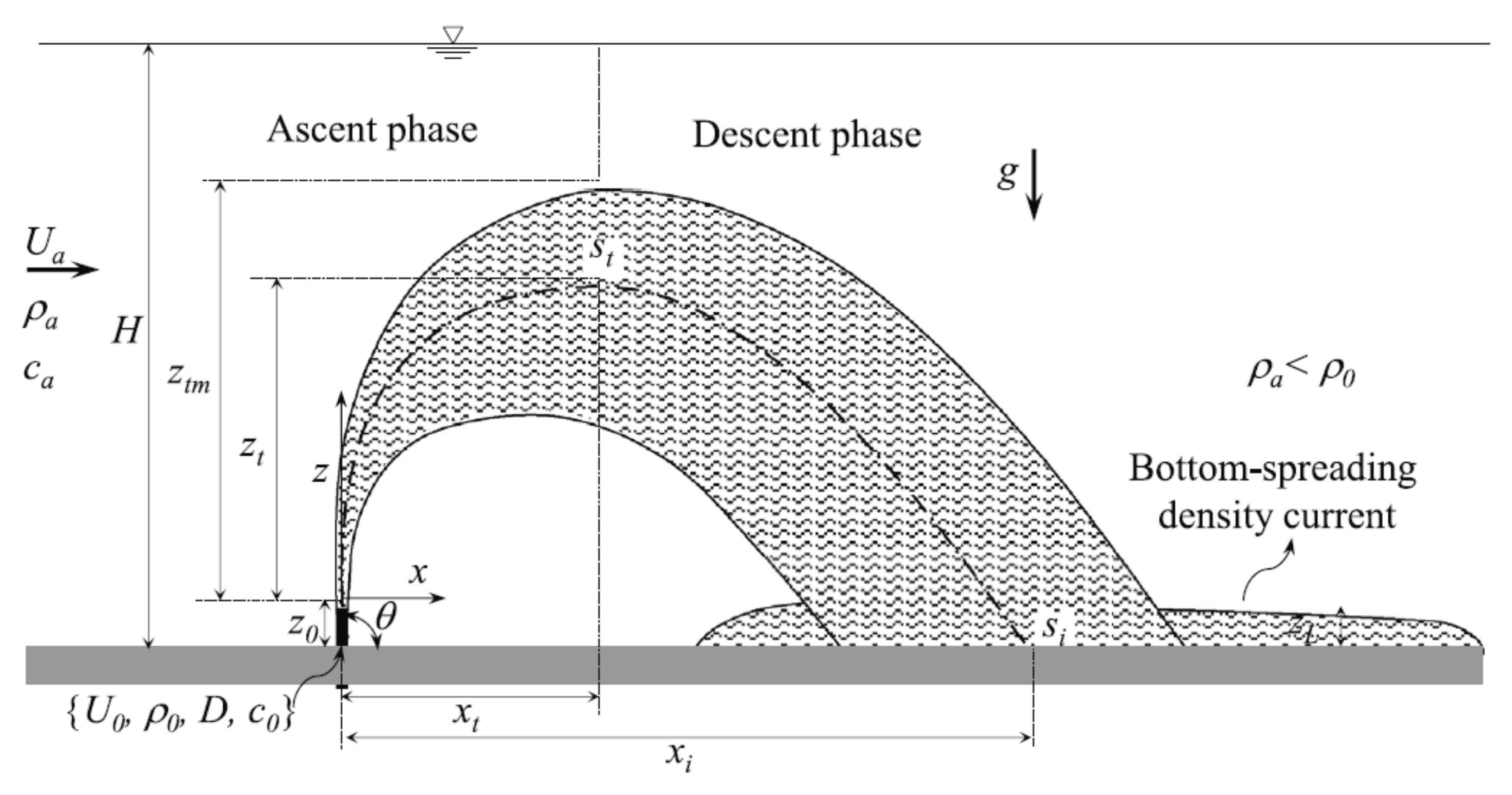
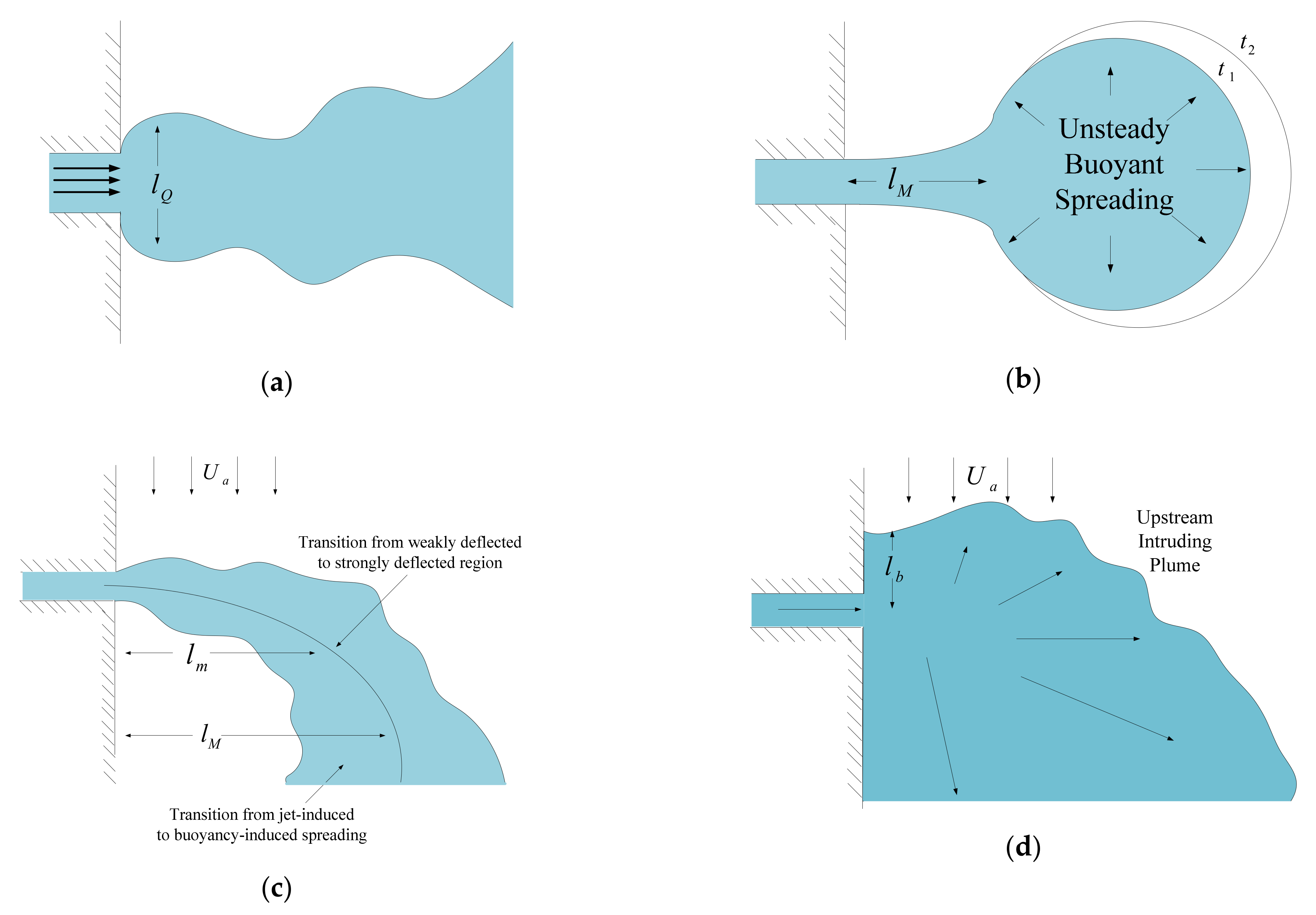
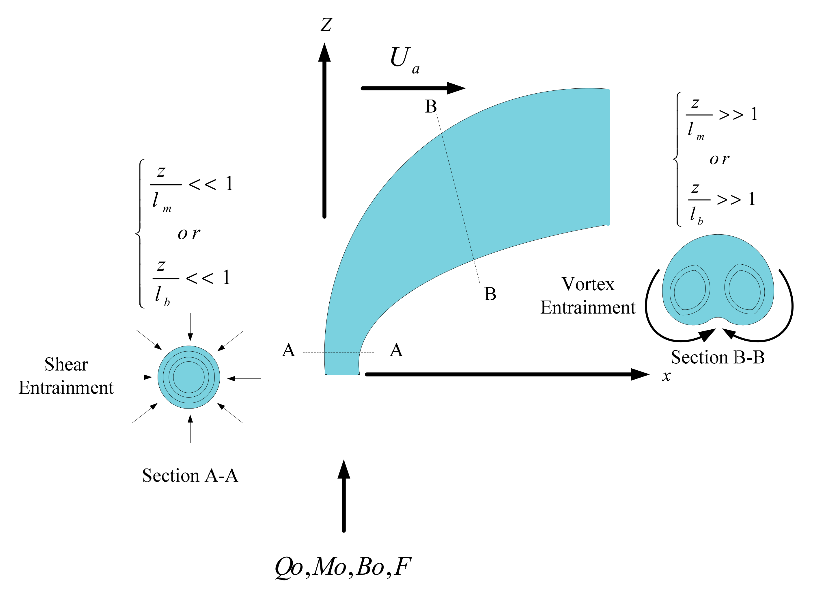
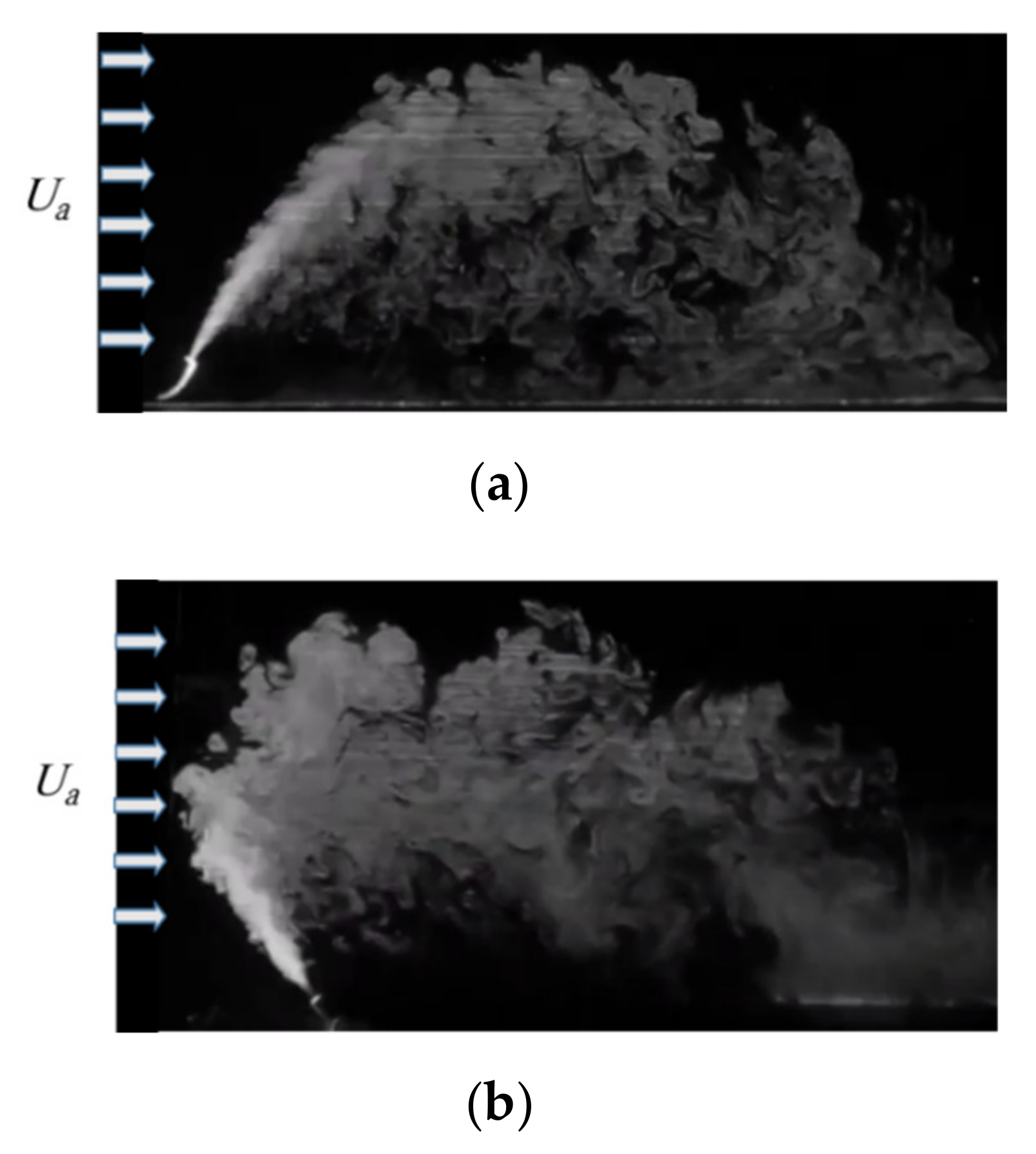
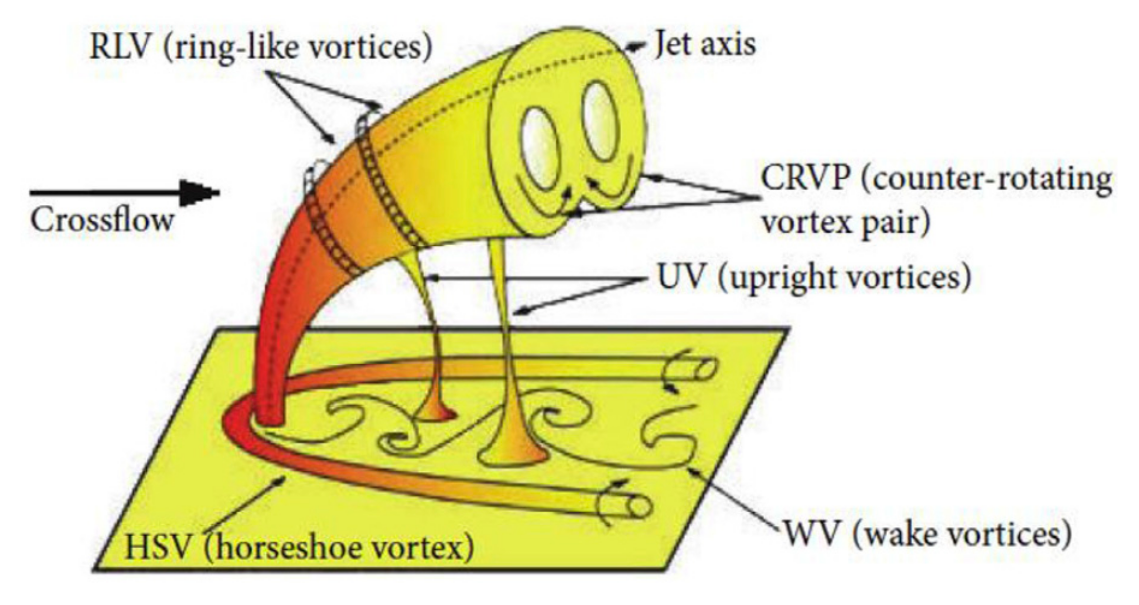
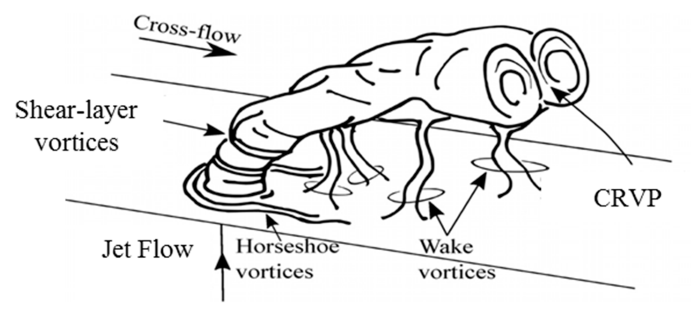
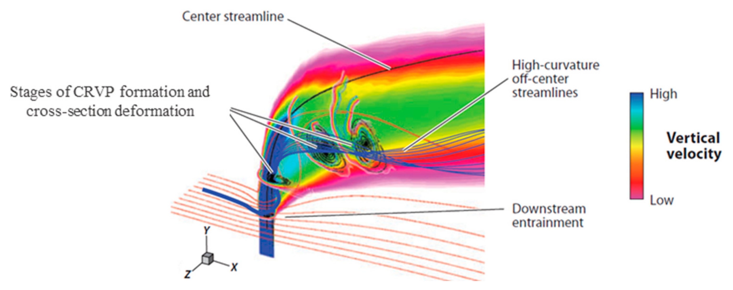
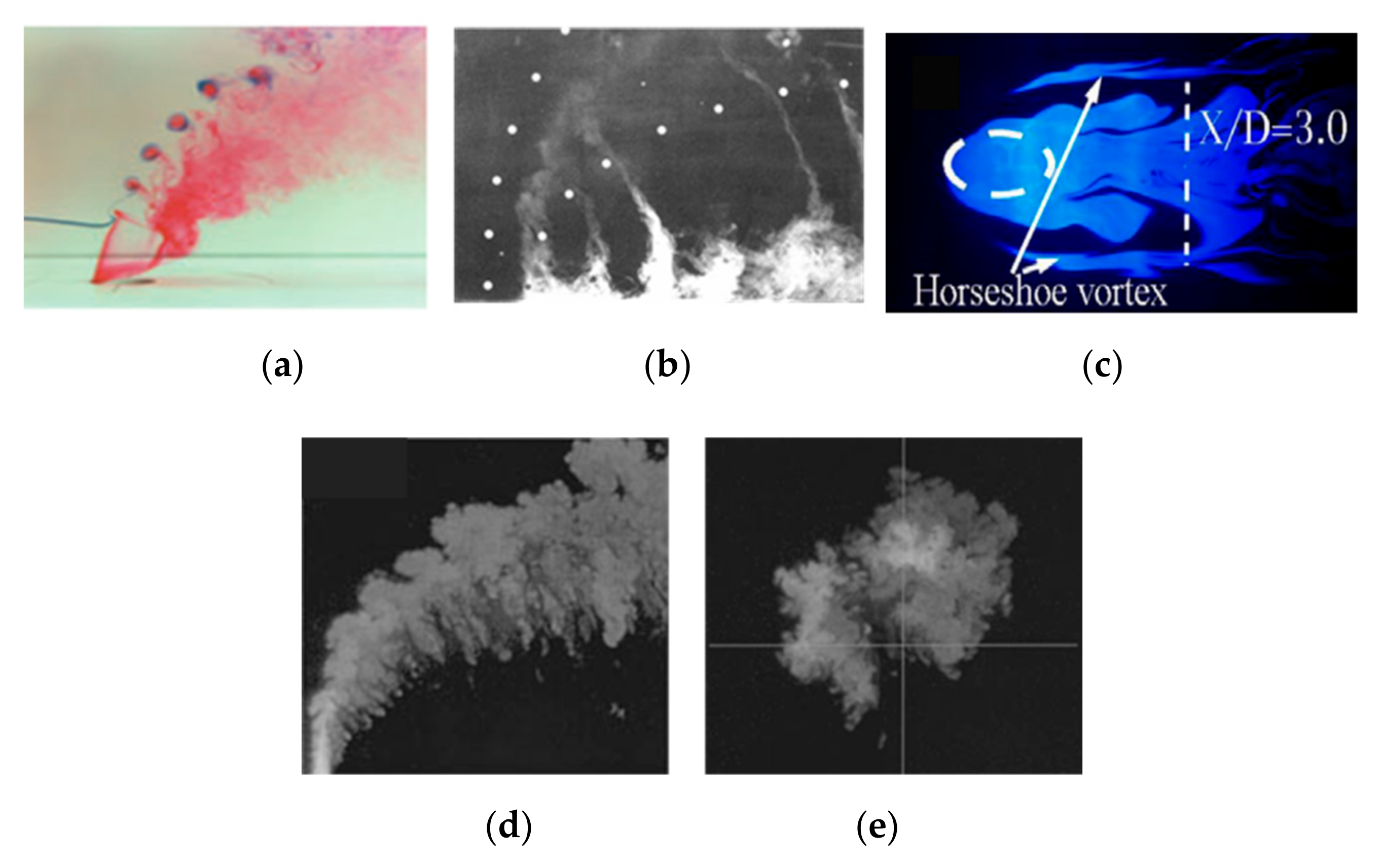
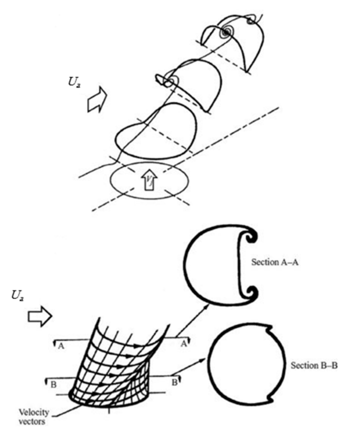
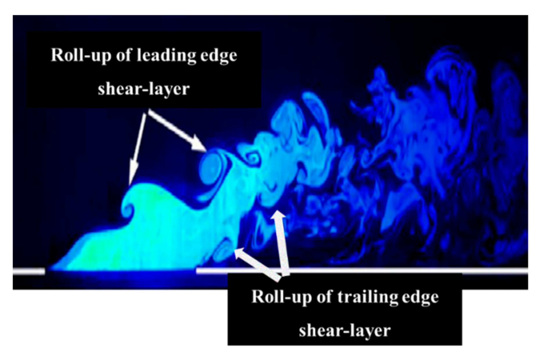
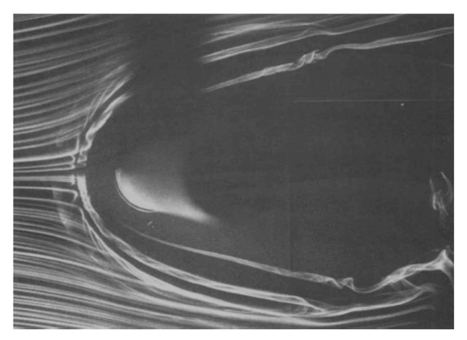
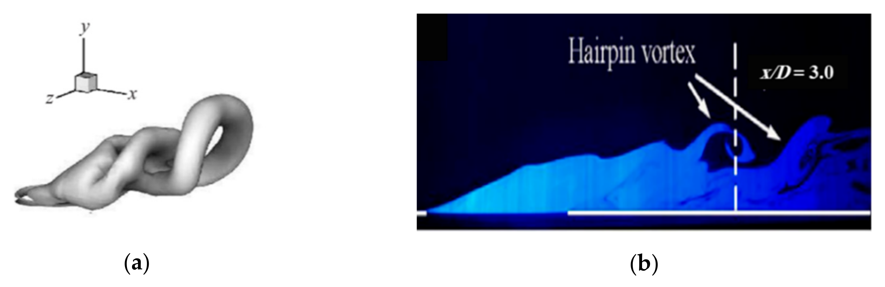
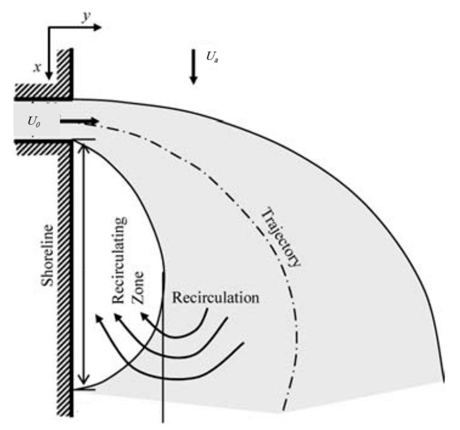
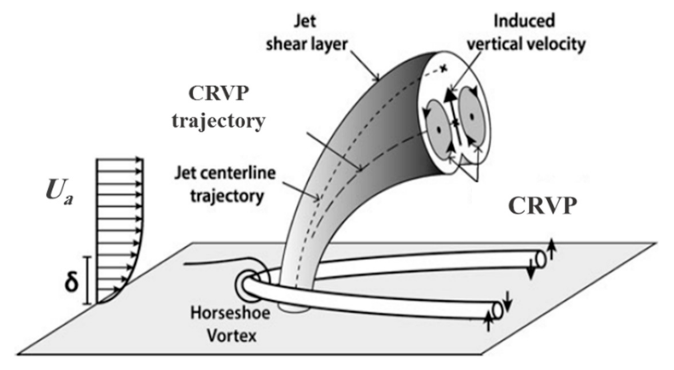
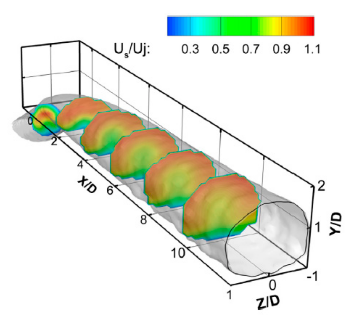
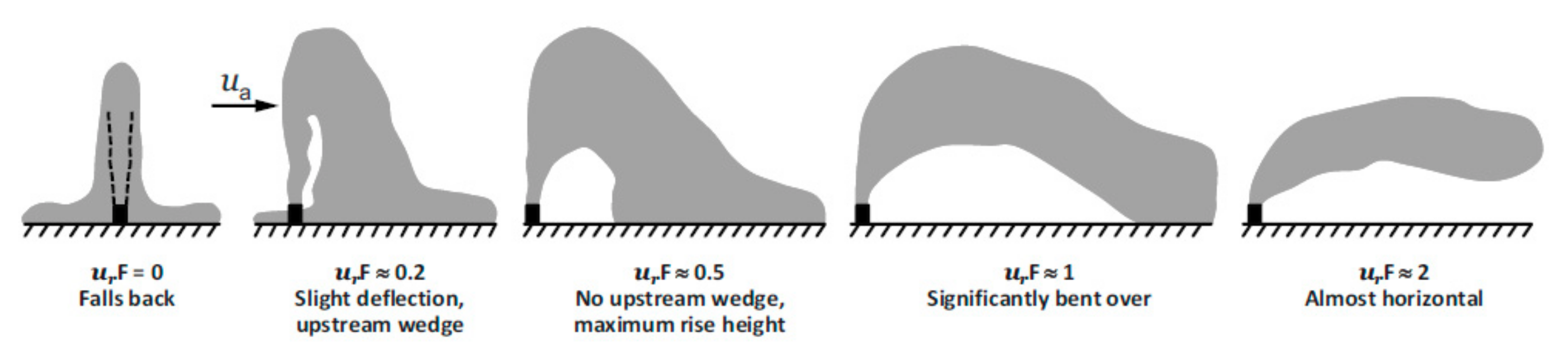
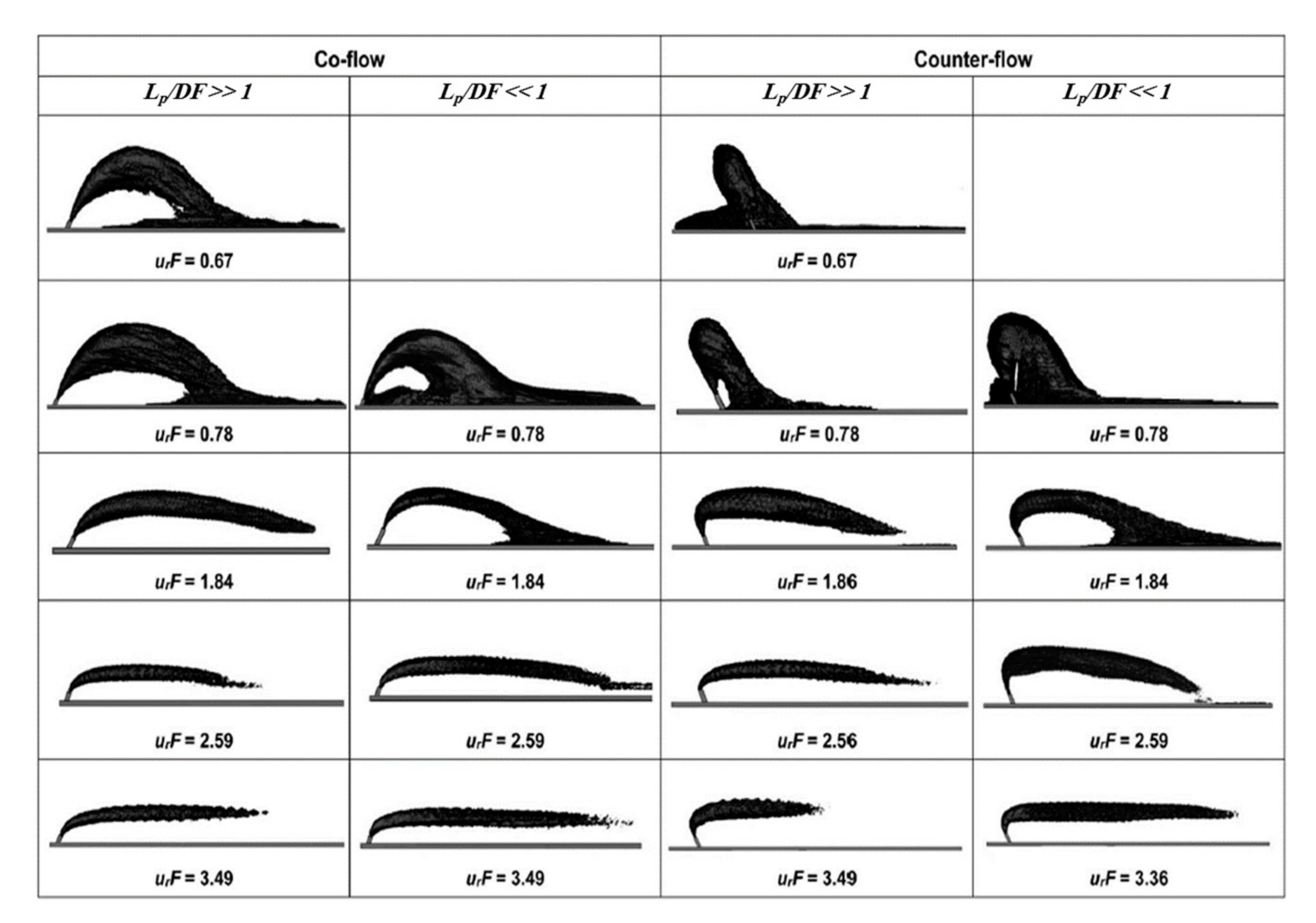
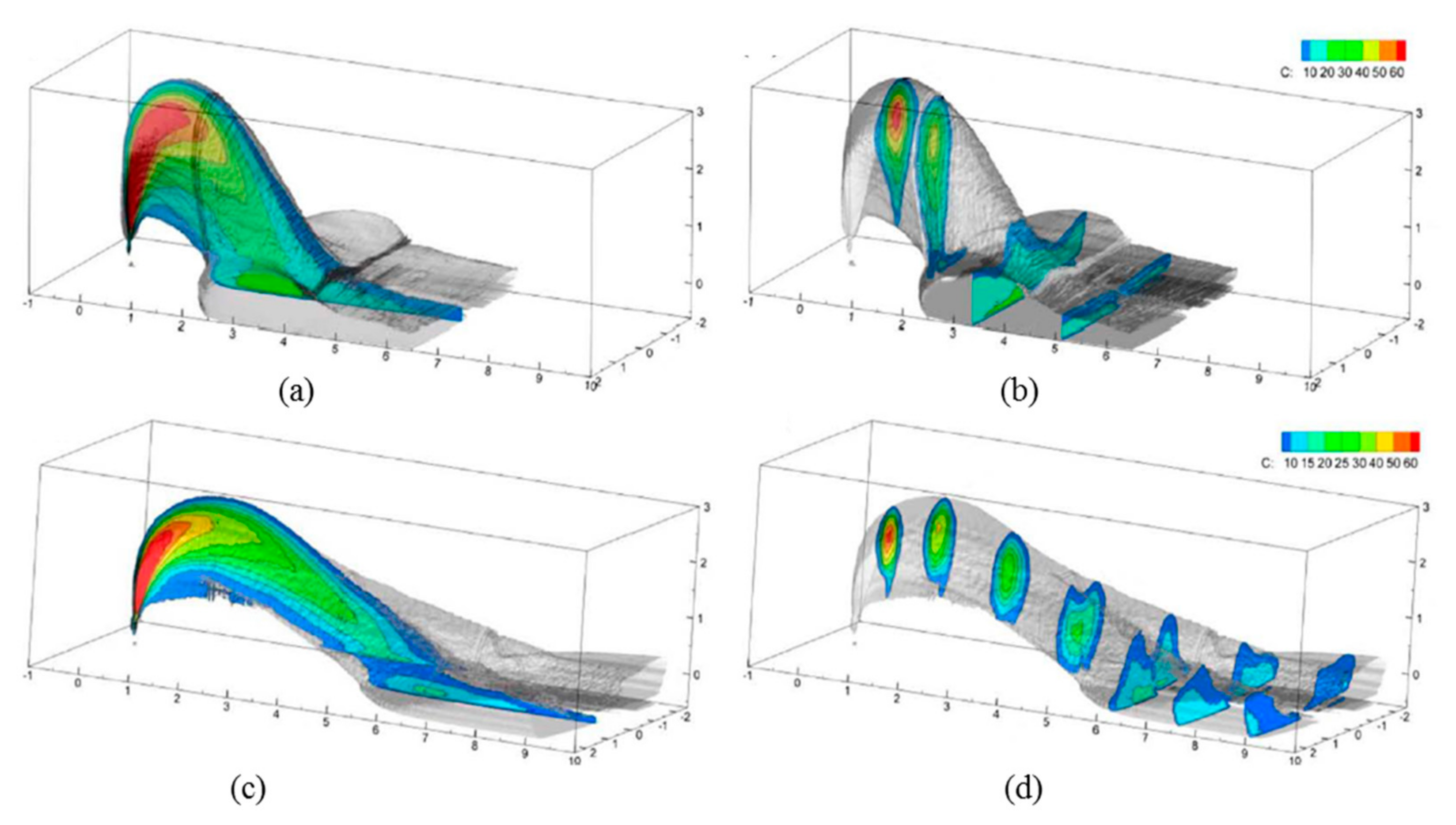
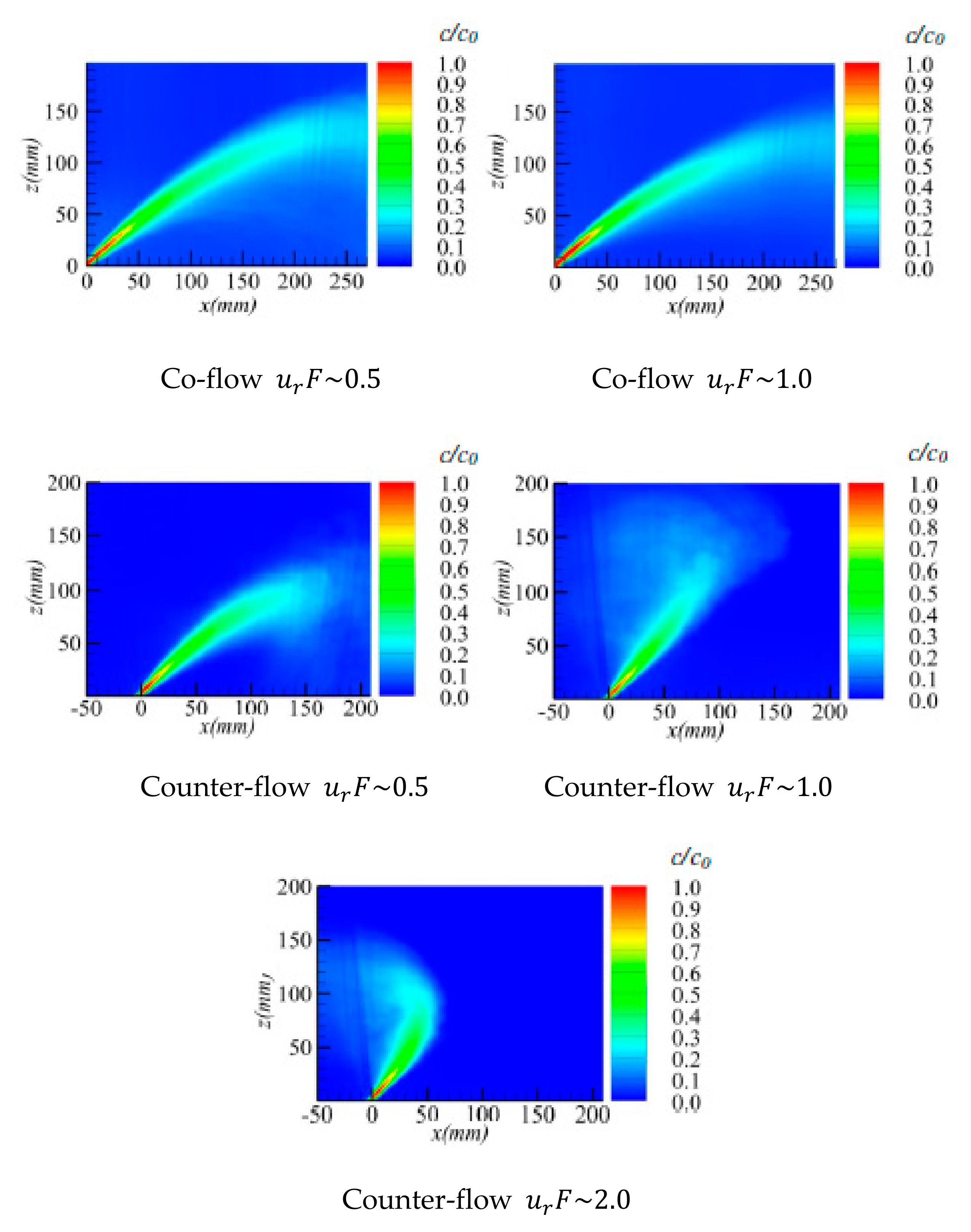
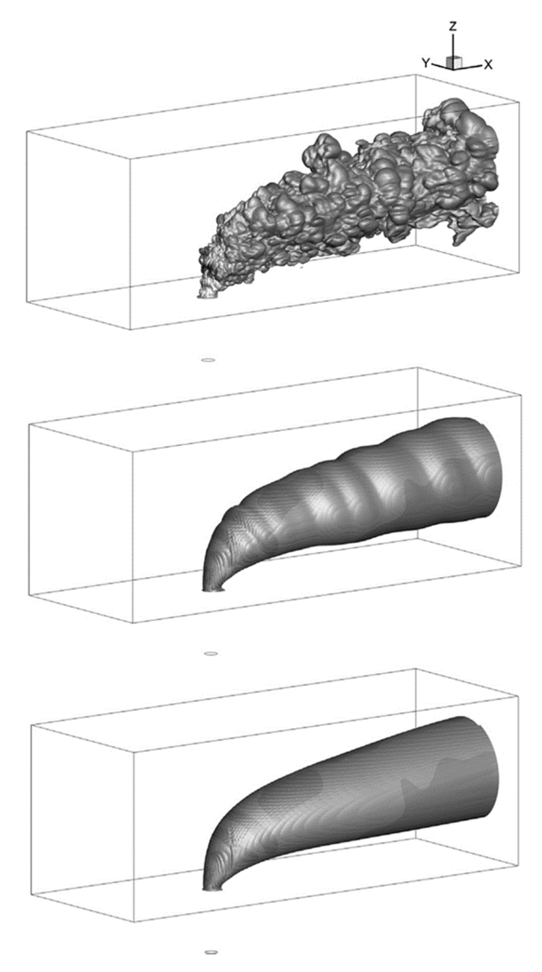
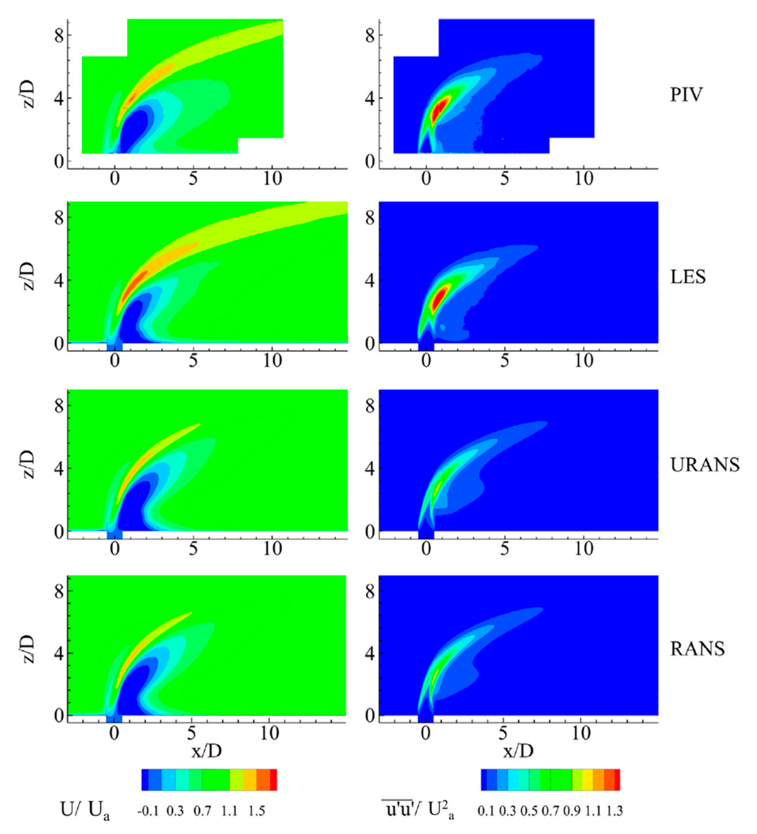
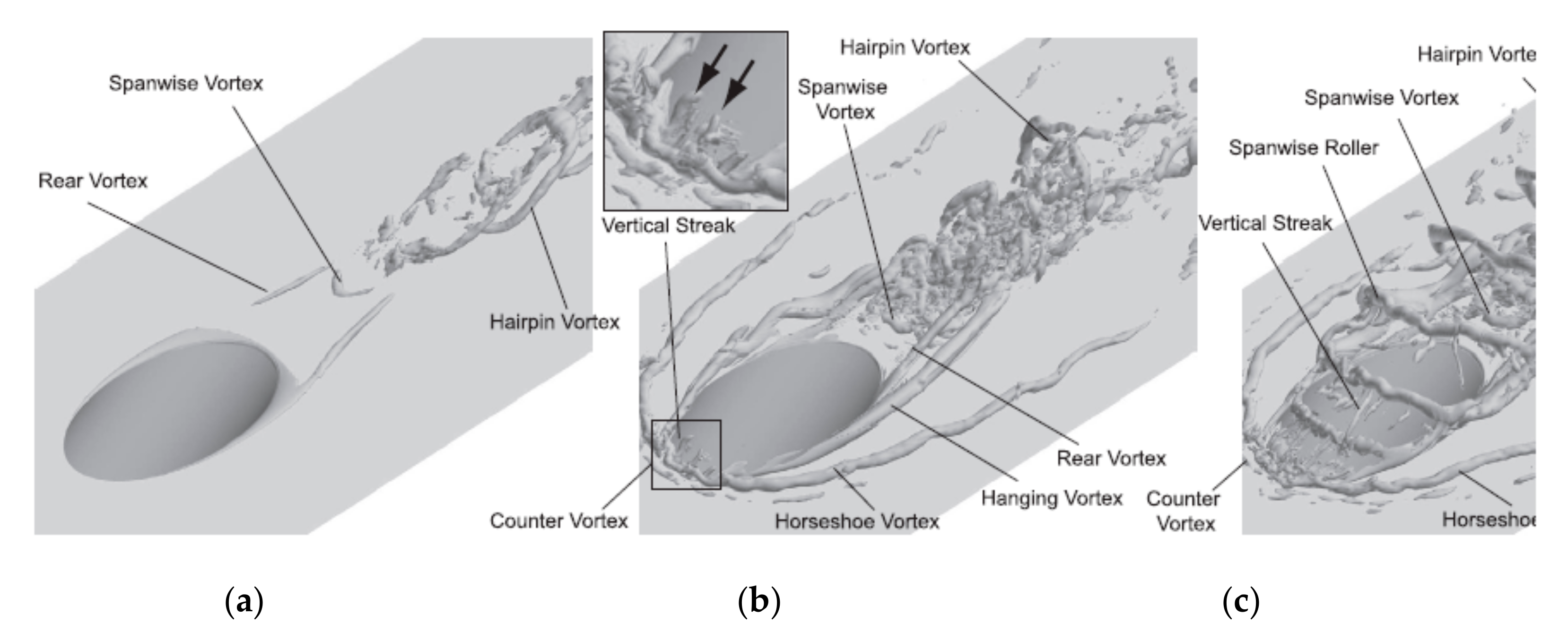
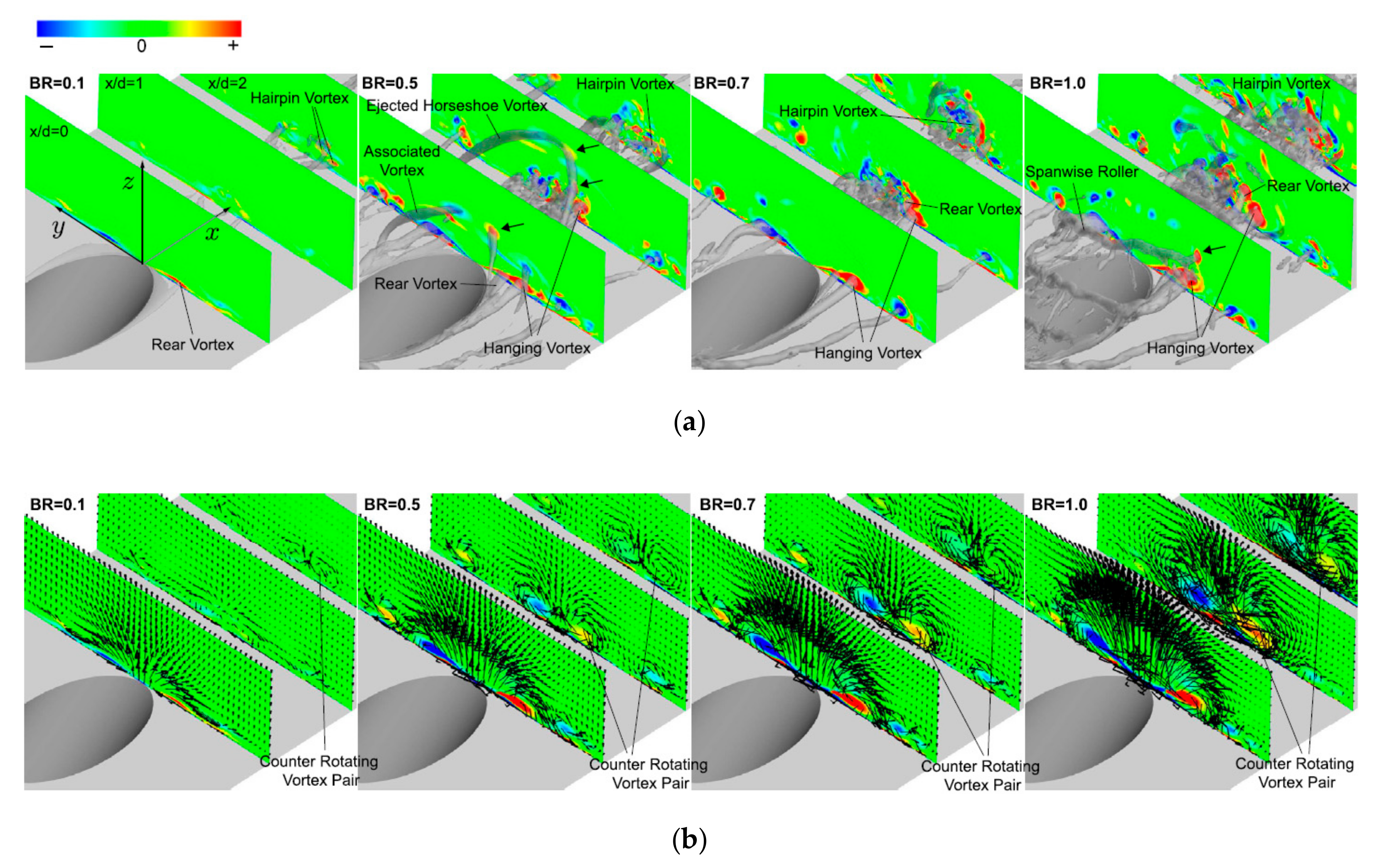
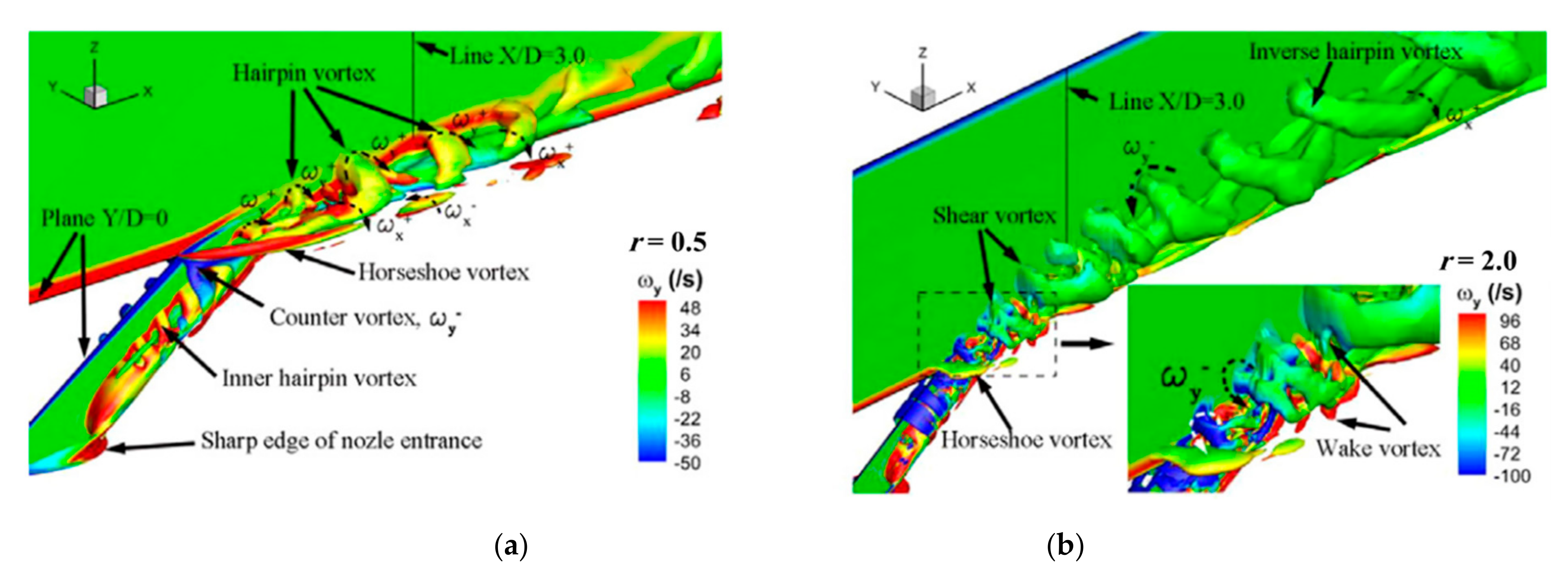
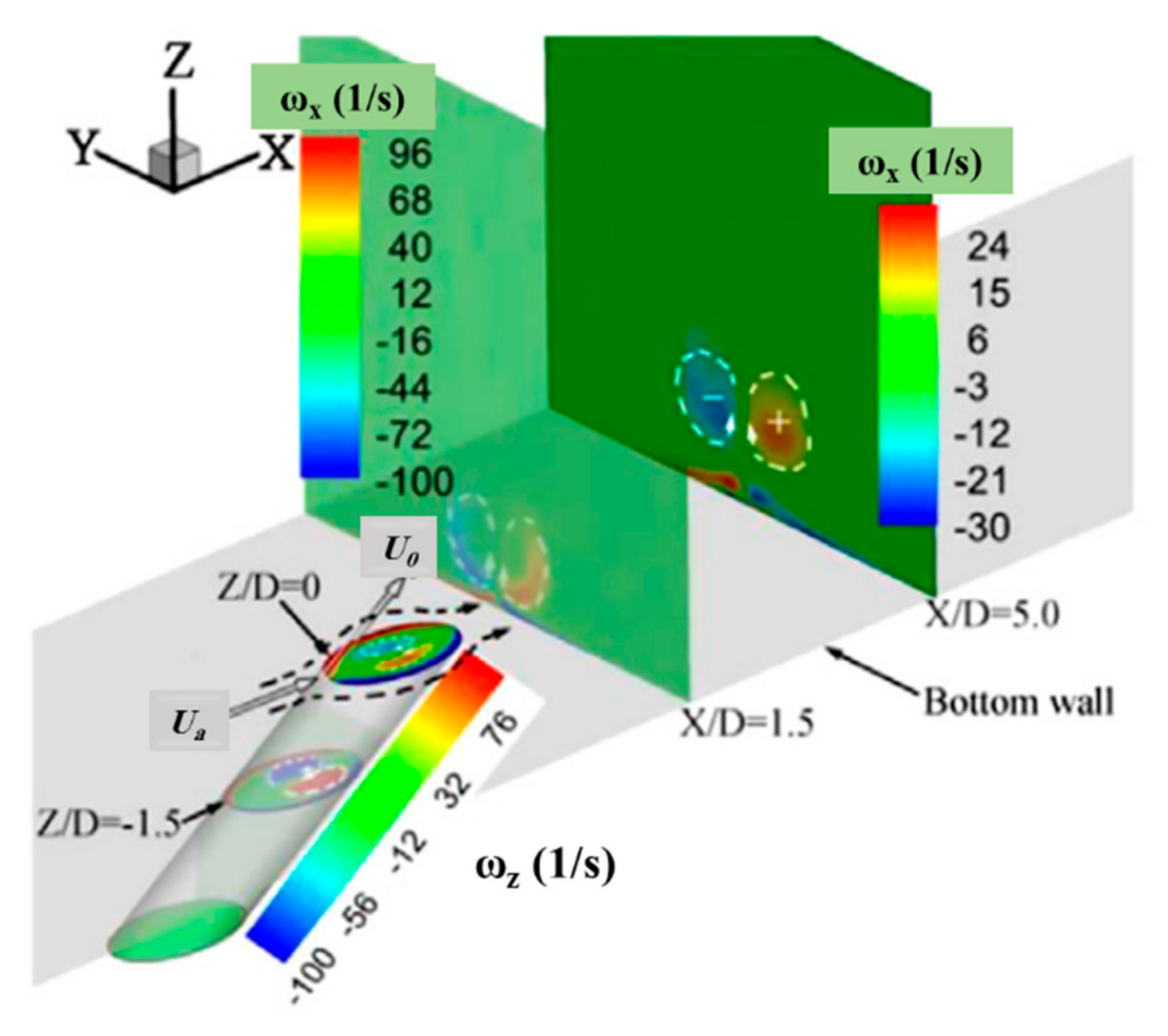
Figure 9.
Interpretation of JICF tilting, folding, and reorientation of shear-layer vortex rings and eventual formation of CRVP taken from Kelso et al. [80].
Figure 9.
Interpretation of JICF tilting, folding, and reorientation of shear-layer vortex rings and eventual formation of CRVP taken from Kelso et al. [80].

Figure 10.
Two independent vortices in the jet shear-layer structure obtained from a laser-induced fluorescence (LIF) visualization [22].
Figure 10.
Two independent vortices in the jet shear-layer structure obtained from a laser-induced fluorescence (LIF) visualization [22].

Figure 11.
Plan view of horseshoe vortex around a cylinder [77].
Figure 11.
Plan view of horseshoe vortex around a cylinder [77].

Figure 12.
Hairpin vortices visualization: (a) hairpin structure for a JICF at r = 1.0 taken from Sau and Mahesh [96]; and (b) instantaneous LIF visualization of hairpin structure at r = 0.5 taken from Dai et al. [22].

Figure 13.
Plan view of recirculating zone formation in a JICF [97].
Figure 13.
Plan view of recirculating zone formation in a JICF [97].

Figure 14.
Schematic of the CRVP and jet centerline trajectories in JICF (δ is the boundary layer thickness) [101].
Figure 14.
Schematic of the CRVP and jet centerline trajectories in JICF (δ is the boundary layer thickness) [101].

Figure 15.
Iso–surface of 5% concentration, with cross-sections perpendicular to the jet centerline (color-coded by jet velocity) [111].
Figure 15.
Iso–surface of 5% concentration, with cross-sections perpendicular to the jet centerline (color-coded by jet velocity) [111].

Figure 16.
General flow characteristics for a vertical dense jet issuing into cross-flow with different values of [39].
Figure 16.
General flow characteristics for a vertical dense jet issuing into cross-flow with different values of [39].

Figure 18.
3DLIF images of a vertical dense JICF for (a,b), (c,d) [39].
Figure 18.
3DLIF images of a vertical dense JICF for (a,b), (c,d) [39].

Figure 19.
Time–averaged concentration contours of an inclined dense jet in co- and counter-flowing currents [113].
Figure 19.
Time–averaged concentration contours of an inclined dense jet in co- and counter-flowing currents [113].

Figure 20.
Comparison the ability of different simulations methods from top to bottom, large eddy simulation (LES), unsteady RANS (URANS), and Reynolds-averaged Navier–Stokes (RANS) for the prediction of coherent structures [126].
Figure 20.
Comparison the ability of different simulations methods from top to bottom, large eddy simulation (LES), unsteady RANS (URANS), and Reynolds-averaged Navier–Stokes (RANS) for the prediction of coherent structures [126].

Figure 21.
Two–dimensional maps of mean velocity component (U/Ua) and specific Reynolds stress component () at the symmetry plane [126].
Figure 21.
Two–dimensional maps of mean velocity component (U/Ua) and specific Reynolds stress component () at the symmetry plane [126].

Figure 22.
Comparison of the vortical structures around the nozzle exit for different values of blowing ratios (BR) including (a) BR = 0.1, (b) BR = 0.7, and (c) BR = 1.0 [92].
Figure 22.
Comparison of the vortical structures around the nozzle exit for different values of blowing ratios (BR) including (a) BR = 0.1, (b) BR = 0.7, and (c) BR = 1.0 [92].

Figure 23.
(a) Instantaneous and (b) time-averaged views of streamwise vorticity (ωx) for BR = 0.1, 0.5, 0.7, and 1.0 [92].
Figure 23.
(a) Instantaneous and (b) time-averaged views of streamwise vorticity (ωx) for BR = 0.1, 0.5, 0.7, and 1.0 [92].

Figure 24.
Spanwise vorticity (ωy) on iso–surfaces of: (a) ∇2P/ρ = 100/s2 for r = 0.5 and (b) ∇2P/ρ = 50/s2 for r = 2.0 [22].
Figure 24.
Spanwise vorticity (ωy) on iso–surfaces of: (a) ∇2P/ρ = 100/s2 for r = 0.5 and (b) ∇2P/ρ = 50/s2 for r = 2.0 [22].

Figure 25.
Time–averaged vorticity contours within the jet nozzle and the vertical planes [22].
Figure 25.
Time–averaged vorticity contours within the jet nozzle and the vertical planes [22].

Table 1.
Definition of the primary flow characteristics of jet.
| Flow Characteristics | Definitions |
|---|---|
| Discharge Volume Flux | |
| Discharge Momentum Flux | |
| Discharge Buoyancy Flux | |
| Jet-densimetric Froude Number | |
| Jet Reynolds Number |
Table 2.
Introduction of the dynamic length scales of jets.
| Types of Scale | Length Scales |
|---|---|
| Jet-to-plume Length Scale | |
| Jet-to-cross-flow Length Scale | |
| Discharge Length Scale | |
| Plume-to-cross-flow (Buoyancy) Length Scale |
Table 3.
Highlighted research efforts regarding CRVP formation origin.
| Origin of the CRVP Formation | Methods | Remarks | Ref. |
|---|---|---|---|
| Tilting and folding of the jet shear-layer vortices | Experimental visualization | Jet to cross-flow velocity ratios ranging from 2.0 to 6.0 and Reynolds number based on the cross-flow velocity and jet diameter in the range of 440 to 6200 | [80] |
| Hanging vortices in the skewed mixing layer | LES | Two different jet to cross-flow velocity ratios (r = 2.0 and 3.3) and low Reynolds numbers based on the cross-flow velocity and jet diameter (Re = 1050 and 2010) | [86] |
| Hairpin vortices | LES | Low blowing ratios * (BR = 0.5 and 1.0) and high Reynolds numbers based on the cross-flow velocity and jet diameter (Re = 11,100 and 22,200) | [89] |
| Interaction of the shear-layer vortices and the cross-flow | LES | Low jet to cross-flow velocity ratios between 0.1 and 0.48 | [90] |
| Origins of the CRVP could somehow be changed with the blowing ratio | Experimental visualization | Different blowing ratios | [91] |
| Hairpin vortices | LES | Comparatively low blowing ratios | [92] |
| Hanging vortices and rear vortices | Comparatively high blowing ratios | ||
| Hairpin vortices | LES and experimental visualization (LIF and PIV) | At relatively low jet to cross-flow velocity ratios | [22] |
| Coherent structures within the jet nozzle | At relatively high jet to cross-flow velocity ratios |
* Blowing ratio (BR) = ρ0U0/ρaUa.
Publisher’s Note: MDPI stays neutral with regard to jurisdictional claims in published maps and institutional affiliations. |
© 2021 by the authors. Licensee MDPI, Basel, Switzerland. This article is an open access article distributed under the terms and conditions of the Creative Commons Attribution (CC BY) license (http://creativecommons.org/licenses/by/4.0/).
Share and Cite
MDPI and ACS Style
Taherian, M.; Mohammadian, A. Buoyant Jets in Cross-Flows: Review, Developments, and Applications. J. Mar. Sci. Eng. 2021, 9, 61. https://0-doi-org.brum.beds.ac.uk/10.3390/jmse9010061
AMA Style
Taherian M, Mohammadian A. Buoyant Jets in Cross-Flows: Review, Developments, and Applications. Journal of Marine Science and Engineering. 2021; 9(1):61. https://0-doi-org.brum.beds.ac.uk/10.3390/jmse9010061
Chicago/Turabian StyleTaherian, Mostafa, and Abdolmajid Mohammadian. 2021. "Buoyant Jets in Cross-Flows: Review, Developments, and Applications" Journal of Marine Science and Engineering 9, no. 1: 61. https://0-doi-org.brum.beds.ac.uk/10.3390/jmse9010061
Note that from the first issue of 2016, this journal uses article numbers instead of page numbers. See further details here.