
A Method to Detect Anomalies in Complex Socio-Technical Operations Using Structural Similarity


Faculty of Engineering and Applied Science, Memorial University of Newfoundland, St. John’s, NL A1C 5S7, Canada
*
Author to whom correspondence should be addressed.
J. Mar. Sci. Eng. 2021, 9(2), 212; https://0-doi-org.brum.beds.ac.uk/10.3390/jmse9020212
Submission received: 7 January 2021
/
Revised: 7 February 2021
/
Accepted: 13 February 2021
/
Published: 18 February 2021
(This article belongs to the Special Issue Human-Automation Integration in the Maritime Sector)
Abstract
:Traditional techniques for accident investigation have hindsight biases. Specifically, they isolate the process of the accident event and trace backward from the event to determine the factors leading to the accident. Nonetheless, the importance of the contributing factors towards a successful operation is not considered in conventional accident modeling. The Safety-II approach promotes an examination of successful operations as well as failures. The rationale is that there is an opportunity to learn from successful operations, in addition to failure, and there is an opportunity to further differentiate failure processes from successful operations. The functional resonance analysis method (FRAM) has the capacity to monitor the functionality and performance of a complex socio-technical system. The method can model many possible ways a system could function, then captures the specifics of the functionality of individual operational events in functional signatures. However, the method does not support quantitative analysis of the functional signatures, which may demonstrate similarities as well as differences among each other. This paper proposes a method to detect anomalies in operations using functional signatures. The present work proposes how FRAM data models can be converted to graphs and how such graphs can be used to estimate anomalies in the data. The proposed approach is applied to human performance data obtained from ice-management tasks performed by a cohort of cadets and experienced seafarers in a ship simulator. The results show that functional differences can be captured by the proposed approach even though the differences were undetected by usual statistical measures.
1. Introduction
Human involvement is crucial to the success of many industrial operations. Many modern industrial operations can be characterized as (complex) socio-technical systems, operations where humans work synergistically with technologies to achieve their goals. A socio-technical system is a label that can be applied to virtually all modern workplaces. Things are usually further complicated by under-specification of work [1], which leads to local adjustments that must be made to accommodate changing and unexpected work conditions. By applying these ideas to industrial workplaces, there is a complexity that makes an assignment of cause and/or blame for workplace accidents seem simplistic or imprecise.
Traditional techniques for accident investigation have hindsight biases. Specifically, they isolate the process of the accident event and trace backward from the event to determine actions/events that contributed to the accident. Contributing factors are often assigned without the study of their significance to successful operations. This is a distinct difference from how the significance of factors is determined in other scientific domains. The observer should also look for the presence of the factor in cases that produce a different effect (success).
This gap in scope for traditional safety management investigations is being addressed by the Safety-II approach [2]. The Safety-II approach promotes an examination of successful operations as well as failures. The rationale is that there is an opportunity to learn from successful operations in addition to failure, and there is an opportunity to further differentiate failure processes from successful processes. One of the implications of increasing the scope of the study is that new models were needed to explain both success and failure, and more information is required to explain the many possible outcomes.
In [3], the authors have developed a framework that uses the functional resonance analysis method (FRAM) to monitor the functionality and performance of complex operations. The method uses the FRAM to model the many possible ways the system could function, then captures the specifics of functionality (tasks, quality/quantity of outputs, and time taken) of individual operational events in functional signatures. The method also uses system performance measurement [4] to measure/compare the overall performance of the operation. By using this framework to monitor complex operations, one can collect data on the overall performance of the operation and the corresponding processes that led to each performance measurement (functionality).
The system performance is typically easy to compare—one should use the same metric for each case and rank them numerically. The functional signatures are more difficult to compare. They contain a lot of information, with many variables that could be/are changing simultaneously. This makes it difficult to have a “controlled” analysis of the variables using conventional statistical methods. There is then a need for other techniques to analyze these functional signatures. Since the functional signatures all demonstrate similarities and differences in comparison with each other, the question becomes how much difference is significant enough to characterize it as “significantly” different from the rest of the group. Or simply, can we detect anomalies in operations by examining their functionality? This paper proposes a method to detect anomalies in operations using functional signatures.
Anomaly detection is an important area of investigation. Anomalies or outliers are observations that fall far from usual or standard behavior. On the one hand, an anomaly can account for a rare signal such as a human error, a banking fraud, or an instrument failure. On the other hand, it can be due to a completely novel process or procedure [5], such that an investigation into this procedure is expected to unleash important aspects for solving the given problem. As a simple example where an anomaly detection algorithm would benefit, consider the case when a medical practitioner treats x number of patients suffering from the same disease. We will assume that a cure for the disease is not known. Therefore, x distinct treatments are administered, one for each patient. The results are not only likely to be different, but there is also an expected competition among the treatments because of the similarity in the overall relief from the symptoms. If many therapies are administered, finding the one that performs better than the others is likely to find the one that falls away from many others. Such is a typical question in clinical research [6].
Another example relevant to the current study is the case of a ship that is tasked to clear ice near a vessel moored in ice. If different people operate the ice management ship, the path it follows around the moored vessel will be different. If there is one best path that minimizes the efforts to achieve the goal of clearing the ice for the longest time then that would correspond to a unique pattern [7] of activities the operator must have performed in order to get the maximum efficiency. If only a few operators (out of many) are found to follow such a rare pattern of activities, such a pattern of activities will not fall into the patterns of activities from usual operators. Anomaly detection is thus a technique to detect such a novel or unique pattern of activities, if there is any, from the given observations.
Human performance data is a record of activities people perform while solving a given task over a given time duration. In particular, human performance data is presented here as graphs obtained from FRAM instantiations. The main contribution of the work is to convert the FRAM based representations of human performance data to graphs such that starting from the beginning of an instantiation at time t = 0, each FRAM function is represented by a corresponding node, and each actual coupling is represented by a separate edge (link) between the involved nodes. As a result, a FRAM instantiation is converted to a graph with multiple edges between nodes representing multiple executions of a single function. In this way, different instantiations of a FRAM model produce different graphs. It is likely that a relatively high variation in graph similarity, if any, must be due to some noticeable difference in the graph structure or the human activities represented originally as the FRAM instantiation. The conversion of a set of FRAM instantiations to a set of graphs makes it possible to exploit graph-theoretic analysis of the human performance data such as comparing different graphs [8], community detection, or estimation of centrality measures for finding important nodes [9,10], which represent functions in the FRAM instantiations, and certainly lay a foundation for estimation of certain interesting aspects of networks; such aspects include the polarization effect, which is useful to see, e.g., how training impacts different groups of people, grouped by some feature like sex or age [11]. The purpose of the present work is to exploit similarity-based clustering (hierarchal clustering) to detect anomalies in human performance data represented in the form of FRAM instantiations. Here, an anomaly is considered as unusual behavior (or pattern of activities) that leads to either valuable or poor (or unsafe) performance.
Section 2 presents a literature review. Section 3 discusses some background concepts related to this study. Section 4 describes the methodology employed for anomaly detection here. Section 5 describes the empirical data and related experiments. Section 6 discusses the results, and Section 7 presents the conclusion and future direction.
2. Related Work
The authors of [12] say that if data are represented as graphs, then graph matching is equivalent to pattern matching. A review of graph-based techniques for pattern matching is presented in [13]. The author reviews 40 years of research and classifies the whole era into three periods. In the first period, classification and learning problems are directly represented in graph space. In the second period, methods from vector spaces, such as a k-nearest neighbor, are transposed so that these methods can be used on graphs. The third period is the one in which graphs are transformed into feature vectors so that methods available as classification and learning methods in vector spaces, such as different kernel machines, can be used on the vector representations of graphs. Similar views are also reported in earlier work [14]. A method for learning graph matching is introduced in [15]. The authors developed an algorithm that estimates how near a graph matching algorithm produces the results when the same graphs are pattern matched by a human being. Based on graph structural properties, a method of clustering is developed and proposed in [16]. This method represents a graph cluster as a graph that preserves the structural properties of all the graphs represented by the cluster. This new graph (i.e., the graph cluster) is called the Weighted Minimum Common Supergraph (WMCS). A clustering algorithm that needs to cluster only a part of the whole data, and whose performance does not suffer due to the size and the shape of the cluster, is developed in [17]. The algorithm is particularly useful when a certain cluster needs to be detected in a sample of graphs, for example, the need to cluster micro-calcification in a mammographic image [18]. A detailed treatment of different distance and similarity measures, the criteria for evaluation of a classification scheme, and different types of clustering, such as graph-based or density-based clustering, are given in [19]. Please consult [20,21,22,23] for a review on techniques related to community detection in networks (or graph).
The study [24] proposes a parallel algorithm for anomaly detection for sequential data. The authors focus on contextual anomalies where the algorithm does not require data labeling. Due to parallelism, the algorithm is fast compared to many previous approaches. The study [25] provides a comprehensive literature review on fraud detection using graph-based approaches. In [26], the authors proposed an algorithm named Glance Algorithm to detect anomalies in attributed graphs based on finding communities within the graph structure and then selecting relevant features per community to detect anomalous behavior. The authors of [27] propose five new measures of graph similarity for web graphs.
The study [28] defines functional resonance analysis space, where a FRAM based analysis can be used in such a way that functions can be assigned depending on the complexity of the system’s level of abstraction. The authors use Rasmussen’s [29] Abstraction Hierarchy to define functions at different levels of complexity of the system. In [30], the authors describe functional variability in FRAM as a quantifiable object by defining rules of variability and their spreading from downstream to upstream functions. The authors use model checking to determine if the state transitions satisfy the rules of variability. In a recent study, [31], the authors analyze over 1700 articles from multiple repositories to see the contribution and scope of FRAM using a protocol developed using the Preferred Reporting Items for Systematic Reviews and Meta-Analyses (PRISMA) approach [32]. The study [33] proposes how a multilayer network can be used to represent FRAM by prioritizing potentially critical functions using network centrality measures such that the transposition is isomorphic to the actual FRAM instantiation. However, the authors did not show how such an isomorphism could be proved. Authors in [34] explained the difficulties of automating processes in the process industries, in particular, due to the nature of coupling and complexity, and developed a FRAM based framework to integrate a human performance model, an equipment performance model, and a first-principal based chemical process model. These components make a hybrid model, the purpose of which is to identify hazards in the process industry. Nonetheless, the FRAM transposition to a multiplex network is essentially important, as many of the FRAM features are preserved, and well-established network analysis tools are at the disposal of the system designer. Detecting anomalies from FRAM data is a new problem and the present work proposes a methodology to represent FRAM instantiations in terms of a graph/network, and then, in line with the idea originally proposed in [35], uses the similarity between graphs to determine if any of the FRAM instantiations (i.e., their graph representation) constitute an anomaly.
3. Background
3.1. Graph Isomorphism
Two graphs G1 and G2 with vertices p are isomorphic if they can be labeled with the numbers 1 to p such that whenever vertex i is adjacent to vertex j in G1, then vertex i is adjacent to vertex j in G2 and conversely [36].
3.2. Graph Similarity and the DeltaCon Algorithm
In [37], the authors propose a rigorous approach to calculate the similarity between two graphs with the same nodes and different edge sets by exploiting the notion of node affinities, where a pairwise node affinity sij of a node i and j is the influence of node i on node j in graph G1. If there are n nodes in G1, a similarity matrix S1 that will hold all values of pairwise node affinities will be of n × n order. Similarly, the matrix S2 keeps the pairwise node affinities for the graph G2. The DeltaCon algorithm [37] calculates the distance between the two graphs G1 and G2, keeping in view the affinity scores of each graph by using the Matusita distance, d, as shown in Equation (1).
where and are elements from S1 and S2, respectively.
The similarity matrix S is computed by using the following equation [37]:
where, I is the n × n identity matrix, D is the diagonal matrix with the degree of node k as the dkk element, and A is the adjacency matrix representing the graph.
The similarity between the two graphs G1 and G2 is calculated using the expression in Equation (3).
4. Methodology
Mathematically rigorous modeling techniques have advantages that come, usually, in the form of techniques for better representations and associated analysis tools. However, all that is available at the cost of various modeling assumptions. FRAM is a modeling technique that gives a modeler the power to represent a process in terms of constituent functions (a group of activities) without making any assumptions [1]. This is much like a computer modeling language, such as Unified Modeling Language (UML), in which a system designer does not bother about what a particular programming environment supports and what it does not. In short, FRAM is a semantically rich modeling environment. Nonetheless, it suffers from very few or practically no formal methods that can be used to analyze different aspects of the modeled process unless a transposition of FRAM is done in some other formal methodology [33]. This section describes a simple approach to considering structural aspects of a FRAM model and associated instantiations in order to develop graphs for different instantiations over a single FRAM model.
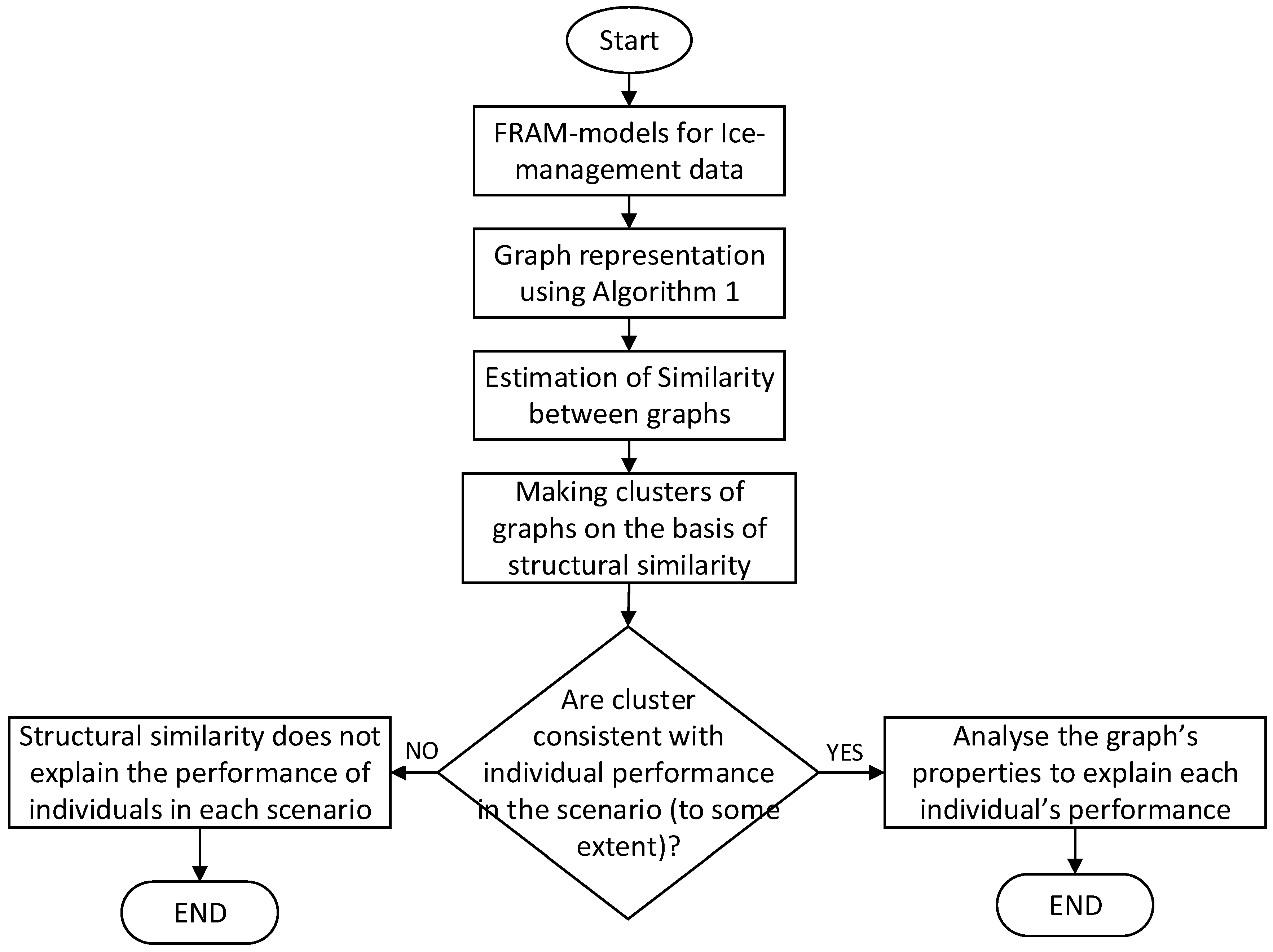
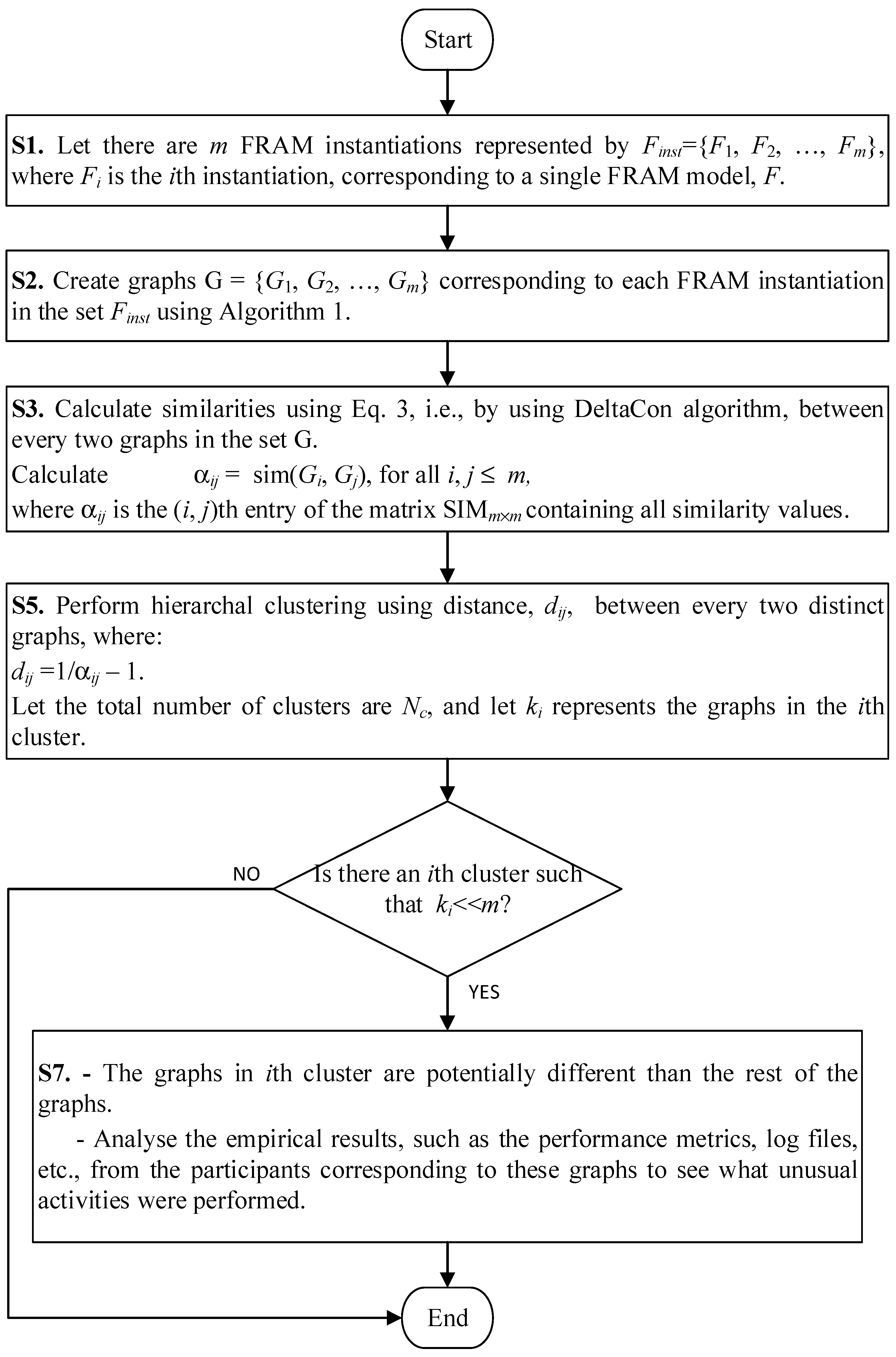
The main objective is to develop a methodology whereby a process that is represented in the form of a FRAM model can be analyzed quantitatively. In particular, the approach developed here focuses on detecting anomalies in human performance data modeled in terms of FRAM instantiations. The basic steps are shown in Figure 1. Because this work involves human performance data represented in terms of a FRAM model, the first step is to obtain a formal representation of FRAM’s instantiations. We propose to convert FRAM instantiations in the form of graphs by using a method described in Algorithm 1 and explained in the following subsections. The graphs obtained from FRAM instantiations can be compared for (dis)similarities using cluster analysis. To this end, the methodology developed here attempts to find out graphs that are marginally different from the other graphs. If there are a total of n graphs (obtained from n FRAM instantiations) to compare and only m << n are found to be dissimilar to the remaining n − m graphs, then only m graphs will be subjected to descriptive analysis. The descriptive analysis involves analyzing the empirical observations, such as considering the performance metrics related to the FRAM instantiations corresponding to the m graphs to determine specific characteristics that may contribute to the dissimilarity of the m graphs.
| Algorithm1 A method to convert a FRAM-instantiation to structurally equivalent graph/network |
| A1: Let F be a FRAM model, and let R represent its instantiation |
| A2: Let there be V= {v1, v2, …, vm} vertices in F, where m is a finite positive integer. |
| A3: Let G be a graph object such that G = G (V, E), where E is defined as follows: |
| E= L ∪ Q = {e1, e2, …, en} is the set of edges in G such that |
| (i) L= {l1, l2, …, lk} is the set of edges in F, and |
| (ii) Q = {q1, q2, …, qp} is the set of edges obtained through R, with k and p positive integers, and, n = k + p. |
| Perform the following steps: |
| S1: Create or add vertices in G corresponding to each functional node in F. |
| S2: Join vertices in G as per the edges in F, i.e., create the edges L among the vertices V in G. |
| S3: do |
| { |
| S4: add edges in G as obtained from the walk-through of R. |
| S5: Ignore directions of edges in G. |
| S6:} while (the end of R) |
4.1. Modelling a Process Using the FRAM
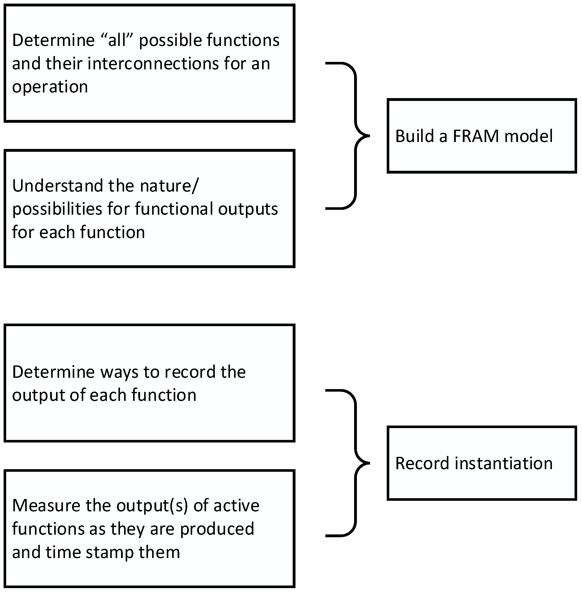
The FRAM is a technique that allows investigation into socio-technical systems to determine how they function. The first part is to build a FRAM model. A FRAM model should be collection functions or activities that can be done to achieve the end goal of the system. The idea is to list all or as many possibilities in this stage. There are many ways to do this: from thinking about the system’s functionality and building the modal as an individual or group of people or interviewing the workers that perform the functions to capture how the work is actually done. Part of describing the system functions is (at least) describing what is produced by the function—the output. There should be some understanding of nature or possibilities of the output(s) at this stage. This work constitutes the building of the model, which is representative of all (or most) of the ways the system can function; however, not all these possibilities are typically used each time the system achieves its goal. Each time the system achieves its goal (or attempts to), which is considered an instantiation, only a portion of the functions may be used, and each function will have a specific output(s). The general understanding of the output of each function (from building the model) will allow for the determination of ways to record each output. Is the output information? Is it a change in speed? Is it a decision? Knowing the answers to these questions will help understand the way to record the outputs. Once you have decided how to record the outputs of the functions, you can record measurements of the active functions and also timestamp the execution of the functions, as the time of functional activity may play an important role in explaining why a certain outcome of the system was achieved rather than another outcome. Figure 2 illustrates this process.
4.2. Representing FRAM Instantiations as a Graph
A FRAM model, or its instantiation, is not a graph/network or flow [1] due to many reasons besides the multiple types of information that each function is able to generate. The main idea here is to convert a FRAM instantiation to a simple weighted graph, or a graph that supports multiple edges (also called a multigraph) by including the number of nodes for functions that were mostly foreground (active) during a typical instantiation process. For a single function, the resonance can only be quantified when the function is executed many times with noticeable variations in performance [38]. Thus, the idea is to make a graph that supports multiple edges from the same nodes for each actual coupling of the FRAM functions represented by the graph nodes. Algorithm 1 describes a methodology to convert a FRAM into a network with (possibly) multiple edges.
In Algorithm 1, only output and input aspects of the FRAM are considered in the conversion to a graph. The other FRAM aspects, time (T), control (C), preconditions (P), and resources (R), are not considered here to obtain an approach that can be used in practical situations. Using a multigraph with six edges per node, it is possible to include the other aspects. However, it is technically difficult to process the information (edge attributes) carried by the edges corresponding to the aspects T, C, P, or R, because the information type is different and the dependency of the function embodied in a node is not explicit in a graph so that the edge attributes could be considered as the function attributes. Additionally, most of the graph algorithms are developed based on a single type of data per graph. An important way to deal with graphs carrying multiple types of information is in social network analysis, where for each type of information, a separate graph is made [10].
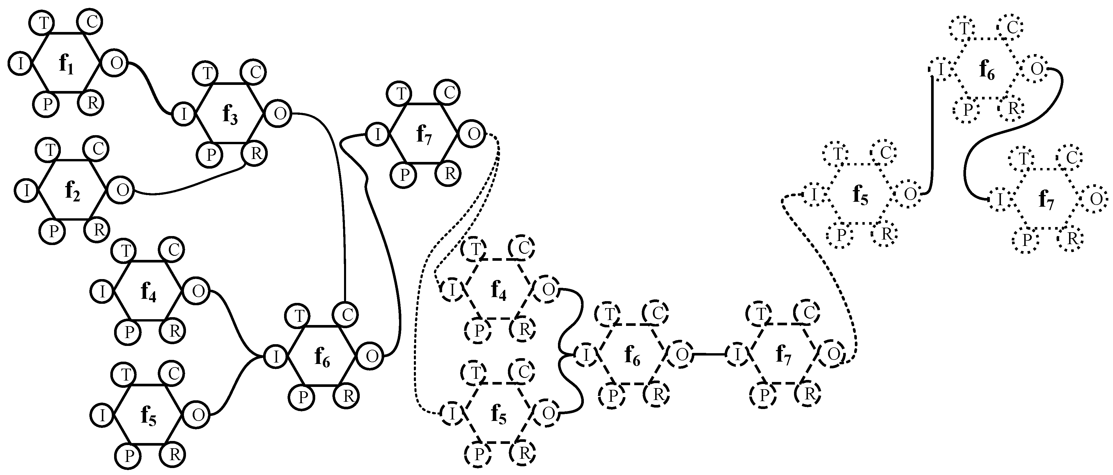
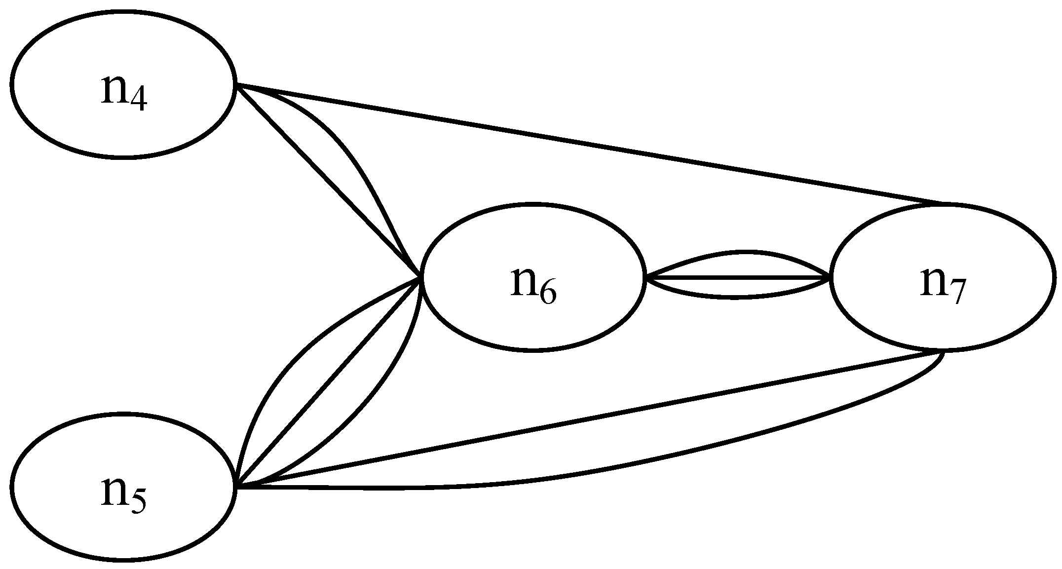
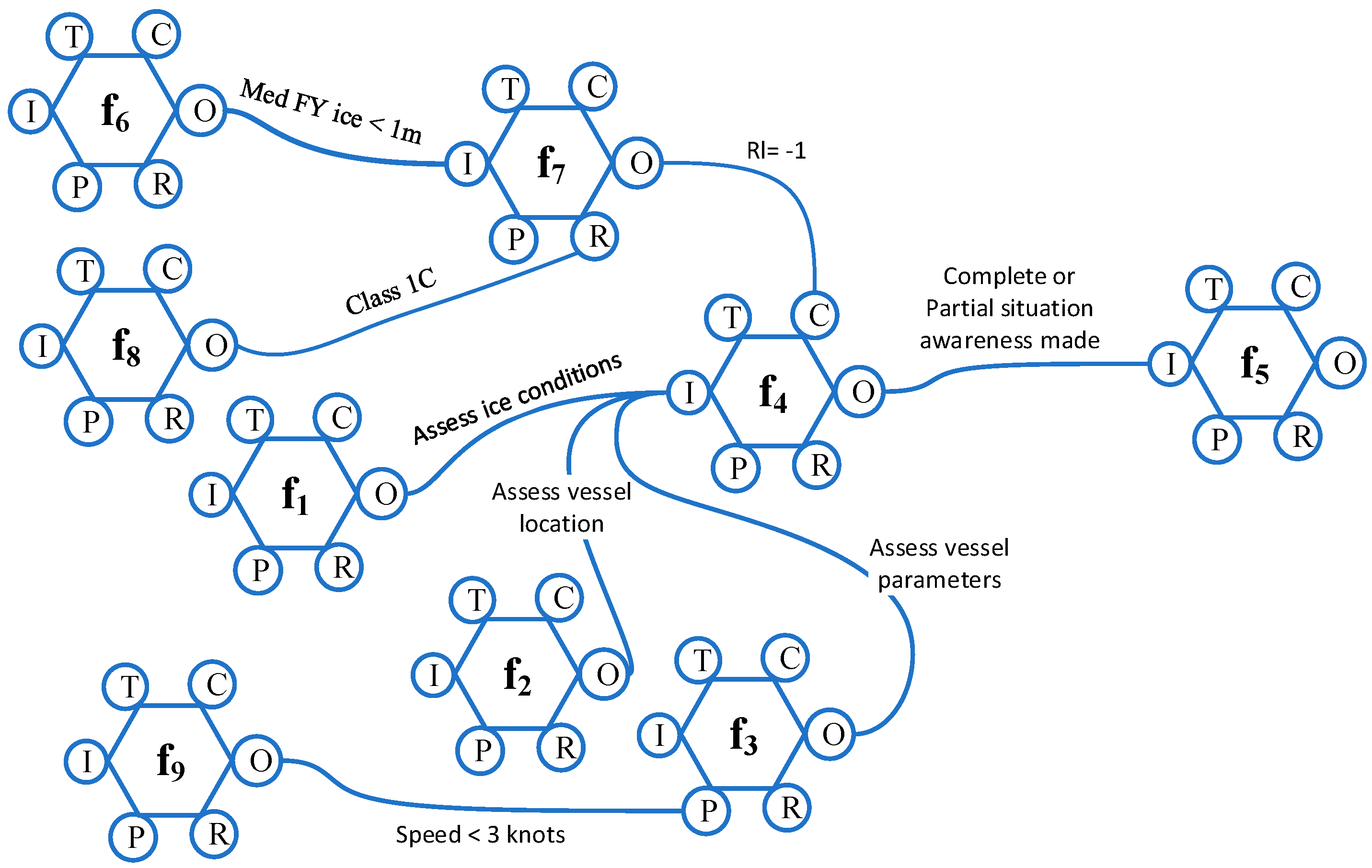
For a particular FRAM instantiation, Algorithm 1 creates a graph with nodes or vertices corresponding to key FRAM functions. These are the functions that play active and dynamic roles in achieving the task. If there are two FRAM functions fa and fb, which are used n times during the entire instantiation, then the nodes na, and nb, corresponding to fa and fb, should be connected by either n edges or an edge with n as the weight. For example, Figure 3 shows a typical instantiation of a FRAM model containing the functions f1, f2, f3, f4, f5, f6, and f7. There are three cycles shown in the entire instantiation where a repetition of a previously used function is activated. In other words, in the FRAM instantiation, functions are performed iteratively. Figure 4 shows a graph obtained after applying Algorithm 1 on the FRAM instantiation presented in Figure 3. Here, nodes corresponding to functions f4, f5, f6, and f7 are included, because these are the nodes that play key roles, and it is here where a change can be seen if the model is instantiated by different people. There may be some functions (such as the functions f1–f3) in the instantiations that contain many cycles (as shown in Figure 4), where only a few cycles make use of these functions (f1–f3). In all such cases, ignoring the inclusion of such functions in the corresponding graph will have little impact on pairwise similarity compared to the case when such functions (f1–f3) are included in the graphs. Examples of such functions may include the background functions, i.e., functions that only have output aspect. For this reason, these functions, which are used only a few times, may be ignored in the creation of graphs from the FRAM instantiations.
4.3. Anomalies
We illustrate the process of converting FRAM instantiations to graphs using data from experiments in which human participants executed an operation that involved driving a ship in a simulator. 71 people participated in the experiments, and each was tasked with executing the same operation, individually. Figure 5 proposes a methodology that has the potential to detect anomalies if observations collected from each participant are presented in a graph format, where the graphs are obtained as described in the preceding section and as illustrated in Figure 4. Let us consider that G1, G2, …, Gm show the graphs obtained from the FRAM instantiations from m participants’ observations. The proposed methodology employs the DeltaCon [37] algorithm (or equivalently Equations (1)–(3)) for the estimation of pairwise similarities between all distinct pairs of graphs. The next step is to make clusters of similar graphs. We use hierarchical clustering for a simple approach using the distance between graphs, and because the sample size for the empirical studies was suitable for hierarchical clustering. The aim is to create clusters based on similarity, , or the distance between the graphs, as shown in Eq. 1. If clusters, say C1, C2, …, Cp, are found containing only a very few graphs, whereas most of the others are found jumbled up in one big cluster, then it is advisable to analyze the graphs within each cluster C1, C2, …, Cp for how the respective participants performed. The analysis may be based on an estimation of each graph’s properties, such as which FRAM function (node) is performed the most, what is the value of the performance metric associated with the function (if there is any), and whether the function was required to be performed at the given time by the participant or not. At the very least, to determine if a certain anomaly is due to a novelty or inexperience, the overall performance may be used. In the present work, overall performance is suggested as an easy criterion for distinguishing expert from poor behavior (both are unusual).
5. Collecting the Human Performance Data for Ice Management Scenarios
5.1. The Ice Simulator
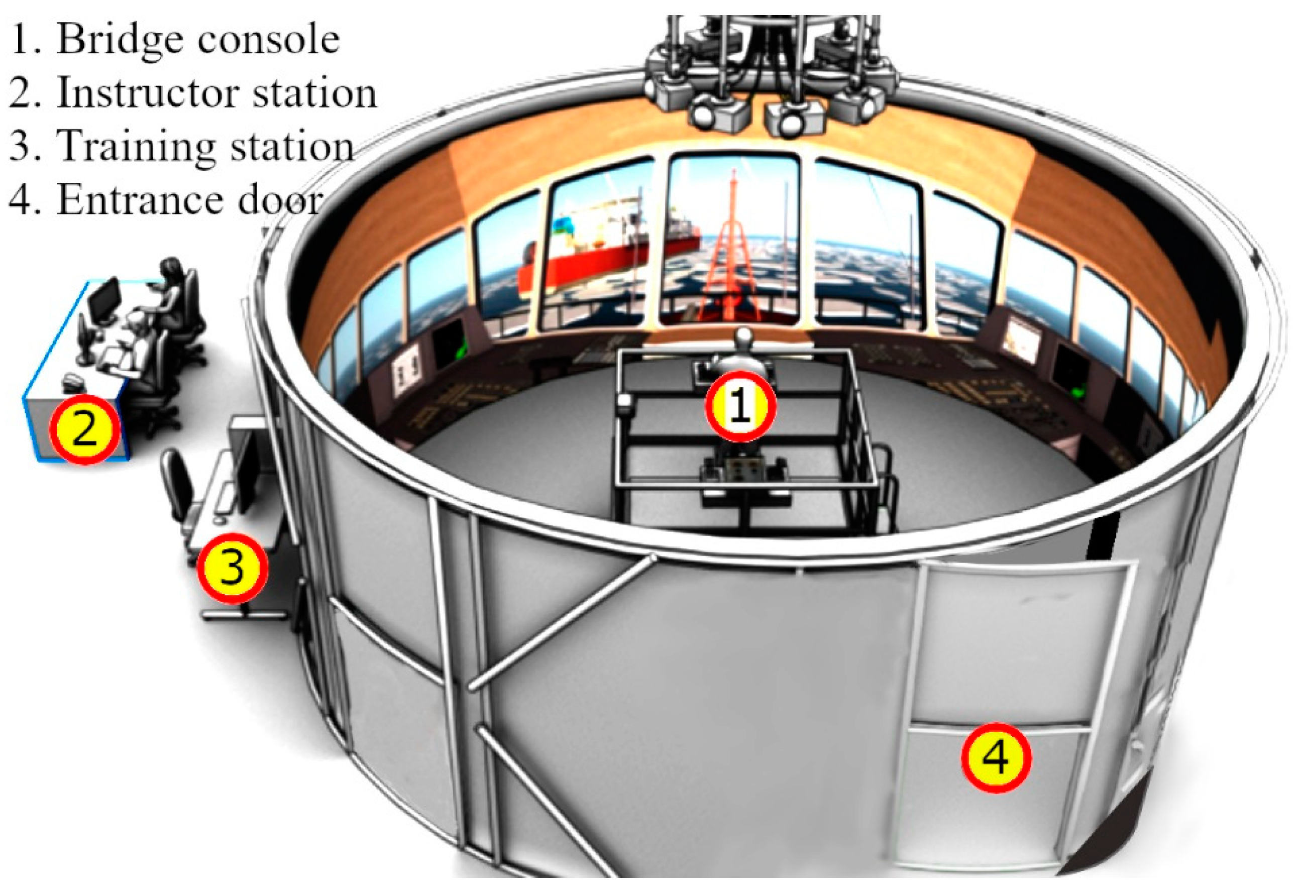
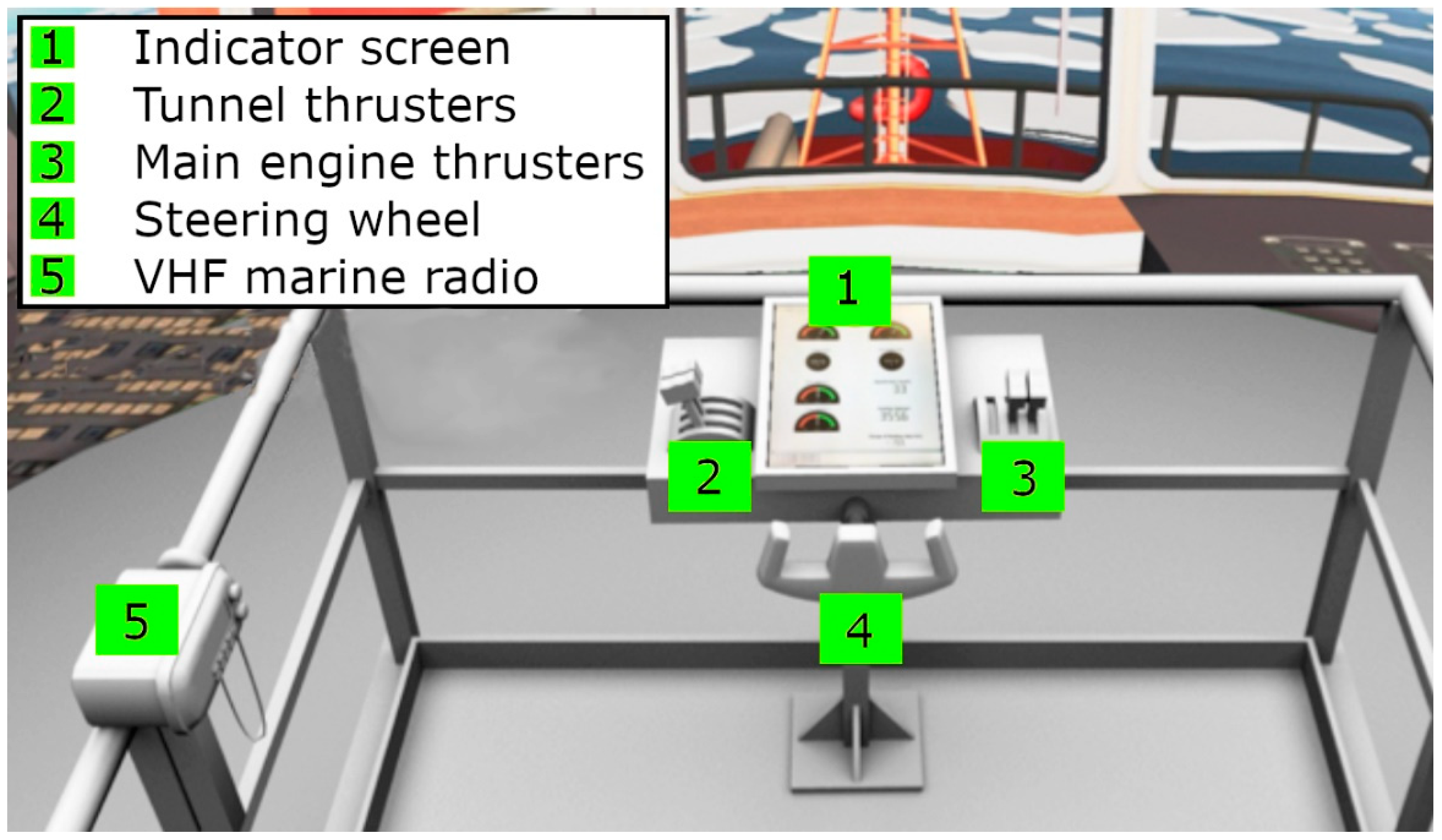
The ice management simulator consists of a bridge console that is a 2 × 2 m platform mounted on a Moog motion bed and is installed in the center of a 360° panoramic projection screen (Figure 6). A 75 m vessel of Anchor Handling Tug Supply type is used in the simulator. It uses two controllable pitch propellers and rudders for propulsion, and forward and aft tunnel thrusters. The design of the bridge console was kept simple to minimize cognitive load and facilitate skill acquisition [39,40]. The bridge console consisted of a fore and an aft console. The four control sticks located on the bridge console (Figure 7) are used to control the power of the two engines and the fore and aft tunnel thrusters.
5.2. The Experiments
The data used here were collected during two separate, but related experiments done in the ship simulator. Experiment 1 [41,42], which was conducted during Fall 2017, investigated the effects of experience on ice management performance. Experiment 2 [43,44], which was conducted from November 2018 to April 2019, investigated the impact of training on ice management performance. All participants performed three habituation scenarios at the beginning of the respective experiments. The purpose of habituation scenarios was to give the participants familiarity with the controls, simulator, and the virtual environment.
In Experiment 1, a group of 36 (novice) cadets and (experienced) seafarers participated. They conducted two thirty-minute ice management operations in the bridge simulator. Two independent variables—ice concentration and experience level—were used in that study. The low level of ice concentration was set to 4 tenths, and 7 tenths, where 4 tenths is a low concentration, and 7 tenths is a high concentration level. The low-level experience category consisted of 18 cadets enrolled in a nautical studies program with 0–3 years at sea. The high-level experience group consisted of 18 seafarers (masters and mates) who had 20 ± 10 years of experience at sea. The performance of participants suggests that, on average, experienced seafarers perform better than inexperienced cadets. However, high variations in the results were also found, as reported in [41,42].
Experiment 2 introduced a training curriculum based on Experiment 1’s findings and the training guidelines proposed in the IMO Polar Code [45]. The learning objectives included (i) the effect of the three ice management techniques, which were learned from Experiment 1, called pushing, prop wash, and leeway; (ii) the effect of recommendations of the Polar Operational Limit Assessment Risk Indexing System (POLARIS) for speed in ice [46]; and (iii) how to keep the lifeboat launch zone clear of ice for emergency evacuation. The total sample size for Experiment 2 was 35. All participants were (novice) cadets from the same nautical studies program as the cadets who participated in Experiment 1. Participants were divided into two groups—G1 and G2—based on training exposure. G1 contained 17 participants who received one training session of 1.5 h length and three practice scenarios. These scenarios dealt with low ice concentration equivalent to 4-tenths of ice concentration. G2 received two training sessions of three hours length and practiced six scenarios under severe ice conditions equivalent to 7-tenths of ice concentration. In both experiments, the maximum time interval for which the lifeboat launch zone was clear of ice during the full 30-min scenario was measured per participant and is considered as the performance metric. This time duration is called Lifeboat Total Time Clear (LTTC).
5.3. Ice Management Scenarios
In both Experiments 1 and 2, participants completed two different 30-min ice management scenarios to show their skills at the given tasks. The first scenario was related to keeping the area around a moored vessel unit clear of ice, and in the second scenario, the participants were asked to clear the ice away from an area around one of the moored vessel’s lifeboat launch zones so that evacuation can be deemed possible. The first scenario is called the precautionary ice management scenario, and the second is called the emergency ice management scenario. As there were two ice concentration levels (4-tenths, and 7-tenths) and two different ice management scenarios (precautionary and emergency), there were a total of four different testing scenarios in the experiments. The present study uses the data collected from only the emergency ice management scenario for validating the proposed methodology of detecting anomalies in ice management activities.
5.4. A FRAM Model for Representing an Emergency Scenario
To build the FRAM model (Figure 8) and instantiation for the dataset (Experiments 1 and 2) used in this paper, the work from [47] was used. The FRAM model was originally created by interviewing ship captains that were published in [48]. The model was originally created for a full-scale shipping operation, so the model was larger. The model size was reduced to only include functions that could be measured in the ship simulator for simplicity of presentation. Performance from each participant in the experiment was recorded as an instantiation and the log file from the ship simulator was used to track the outputs of the functions.
The area beneath a vessel where lifeboats are launched needs to be clear so that there is no obstruction for launching a lifeboat in case of an emergency evacuation. Participants in the emergency ice management scenario were asked to clear the area of ice so that emergency evacuation can be performed.
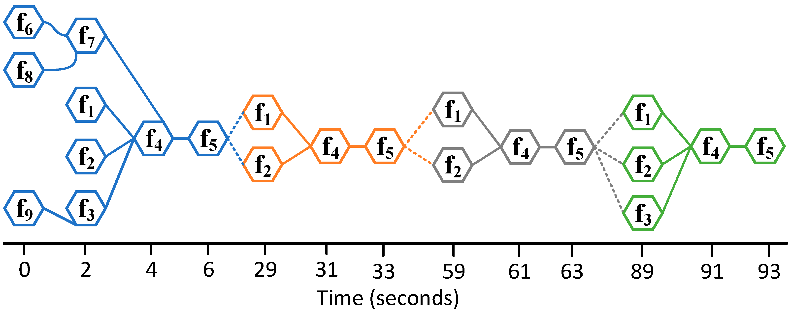
It is observed from Experiments 1 and 2 that participants’ activities can mainly be divided into two categories: observing the situation and then acting accordingly. These activities are shown as function 1 (f1), function 2 (f2), function 3 (f3), function 4 (f4), and function 5 (f5) in Figure 8. The f1 means to observe ice conditions. Here, participants watch how much ice is cleared from the target area, and where in the region the ice floes are present. The input is the visual that the participant watches in the simulator; the output is the volume of floes in the target area. The f2 means to assess location and surroundings. This function calculates the location of the vessel (the icebreaker) in geographical units. Again, this information is provided to the participant in the form of latitude and longitude on the simulator console. The function f3 is the activity that employs monitoring the vessel parameters. Two vessel parameters are used here, the speed and the heading. Both, as explained in Section 5.1, are controlled parameters. The values are shown on the simulator console. These three activities, f1, f2, and f3, focus on observing the situation. The f4 involves understanding the situation so that better decisions can be made. Inputs to f4 are the outputs from the functions f1–f3. The function f4 is a cognitive function and, therefore, during the experiment, we relied on watching what was done after the execution of f1–f3 to get an idea of what might have been done in f4 in terms of an understanding of the situation given the values of f1, f2, and f3. For example, consider the activities performed by a participant during the 89th second of the scenario reported in Figure 9. The output of f1 here was 4.99 tenths. The output of f2 was latitude = −146.38, longitude = 60.49. The f3 outputs the speed as 2.697 knots, which is under the threshold of 3 knots—the safe speed. Based on these values, the participant understands that the currently employed strategy is good enough. Based on this result from f4, the participant decided (the function f5) not to change the speed now (the speed remained the same from the 89th second to the 333rd second), and the vessel kept clearing the ice along the current path.
Finally, f5 represents activities corresponding to the understanding of the situation in f4. Function f5 is not connected to any other functions in the FRAM model (Figure 8), but it makes connections with f1, f2, or f3 during individual instantiations (see Figure 9). For instance, if it is decided in f5 that only the ship speed needs to be changed, then f5 carries that information as a value over the link and connects the relevant function for observing the speed again, which is f3. Similarly, if a participant decides in f5 to get information about current ice conditions and update the heading, then this information will show as values over the links connecting f5 with f1 and f3, respectively. The functions f6–f9 represent activities that are not dynamic, but they act as either preconditions or control for the connecting (or downstream) functions in the FRAM. The f6 represents the act of “judgment about the ice type”, for example, whether the ice where the ice clearing operation is to be performed is multi-year ice or first-year ice. In the present study, medium first-year ice is used. The function f7 models “computing the ice risk”. Because the study involves only medium first-year ice, the risk index value (RIV) is −1 according to Polar Operational Limit Assessment Risk Indexing System (POLARIS) calculations [46]. The function f8 shows “assignment of the ship classification”. The present study uses a Polar Class 7 (PC7) ship [43] (p. 242).
The function f9 stands for “be aware of vessel capabilities”. With this, the intention was to keep in mind the vessel capabilities, that is, the speed should remain less than 3 knots. This function bears a cognitive load to participants during operation. However, due to simplicity, the function f9 was only assessed at the beginning of the scenario.
Table 1 shows a sample of activities up to 119th second of the participant with code name S51. The series of different activities performed by the participants are identified as functions in the FRAM model. These functions are shown in Figure 8 and are described in Table 1. The process of instantiation involves how each participant performed these functions, what output is produced, which function follows the active function, at what time a function is performed, and how the connections are made, i.e., which aspects are involved in an activity. It is observed that during the 30-min long experiment, each participant uses aspects other than input and output only 2–3 times (out of, on average, 450 activities performed in 30 min); therefore, the present work only takes into account input and output aspects of the functions presented in the model in Figure 8.
5.5. Scenario 1: Emergency Scenario with Mild Ice Conditions
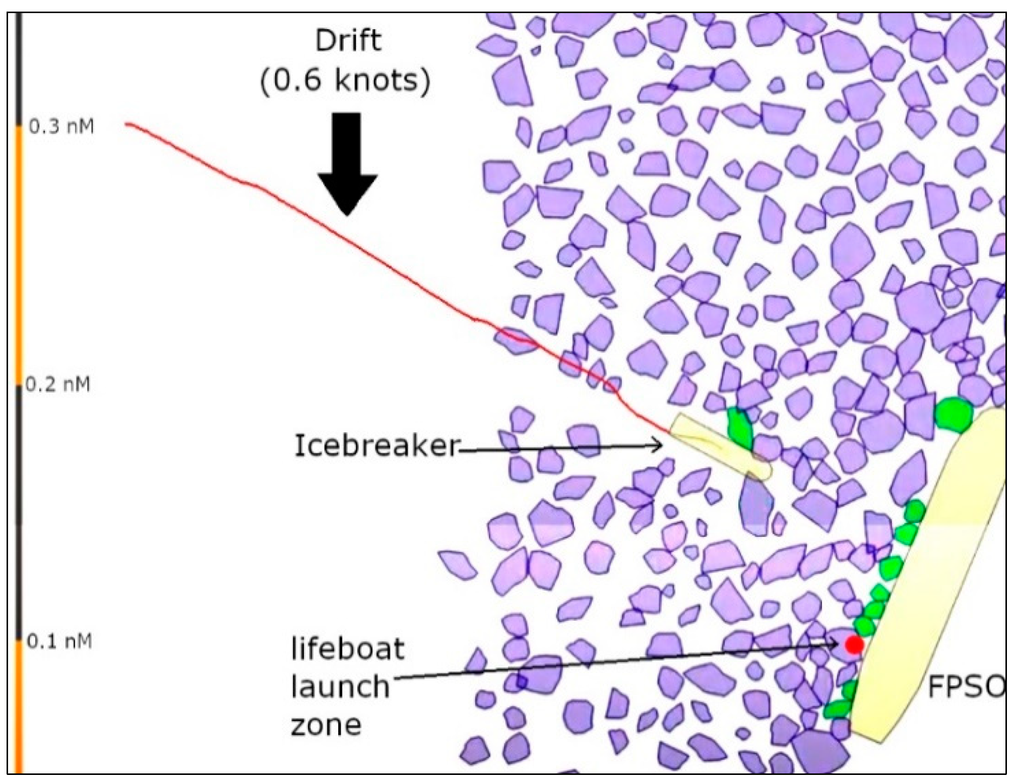
As the emergency ice management scenarios were the same in both experiments (Experiments 1 and 2), we have included results obtained from both experiments, yielding 27 instantiations for the present analysis. In this scenario, the FPSO is in mild ice condition (4 tenths concentration) with an average ice drift of about 0.6 knots (see Figure 10). The participant was asked to clear away the ice from an area below the stern port lifeboat launch zone.
5.6. Scenario 2: Emergency Scenario with Severe Ice Conditions
In this scenario, the participants were asked to clear the ice from the lifeboat launch zone just as they were asked in Scenario 1. The only difference between this scenario and scenario 1 is in the ice conditions, which were set to 7 tenths concentration level (severe ice condition). The ice floe drift was 0.5 knots.
5.7. Graph Representations of FRAM Data
Algorithm 1 has been applied to the data sets obtained as FRAM instantiations in scenarios 1 and 2 as described in the preceding sections. A graph for each of the 61 FRAM instantiations—one for each participant—was generated. For brevity, only portions of the graphs of four participants are shown in Figure 12.
6. Results and Discussion
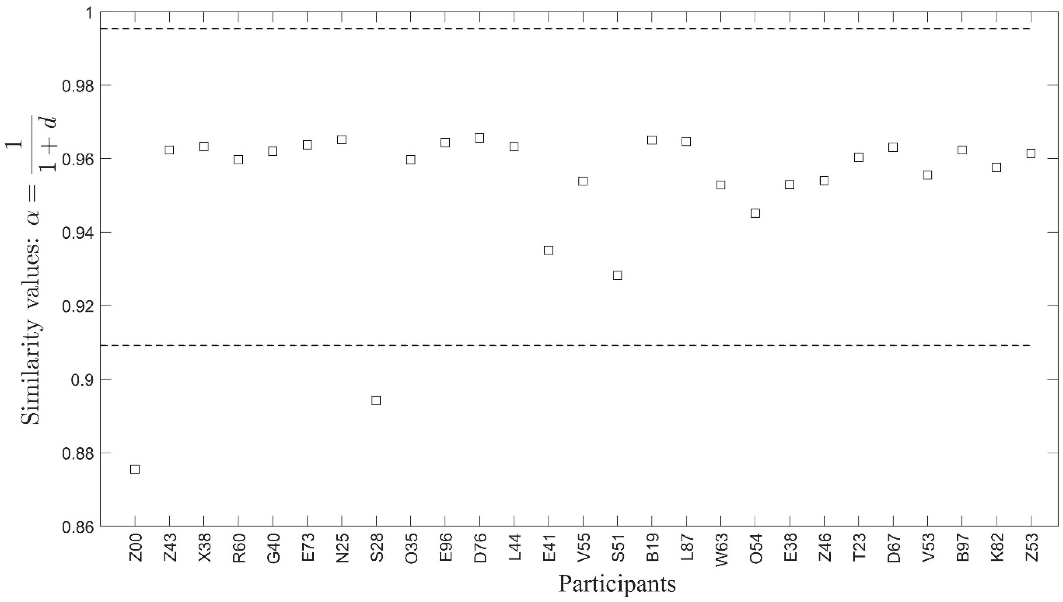
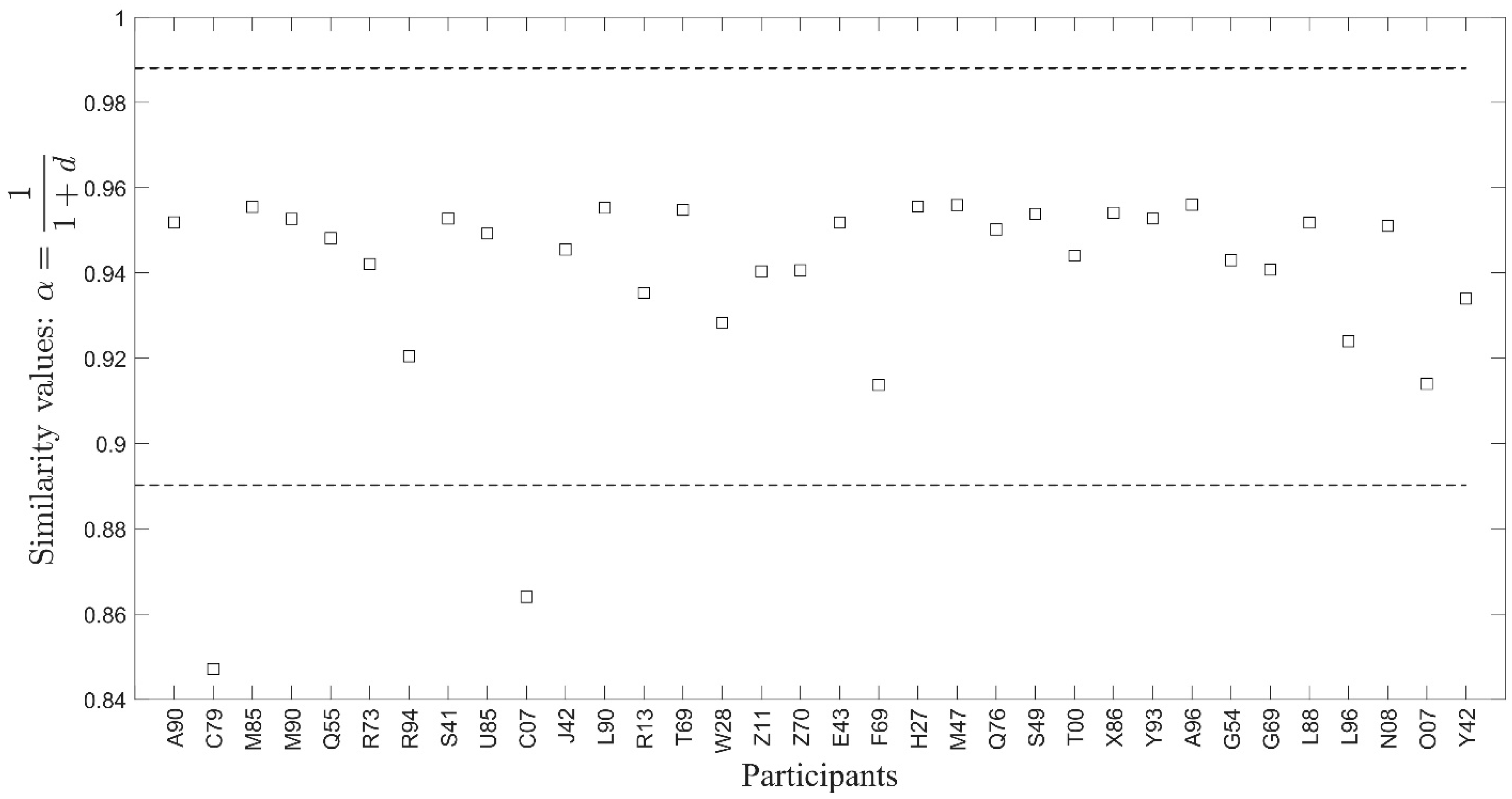
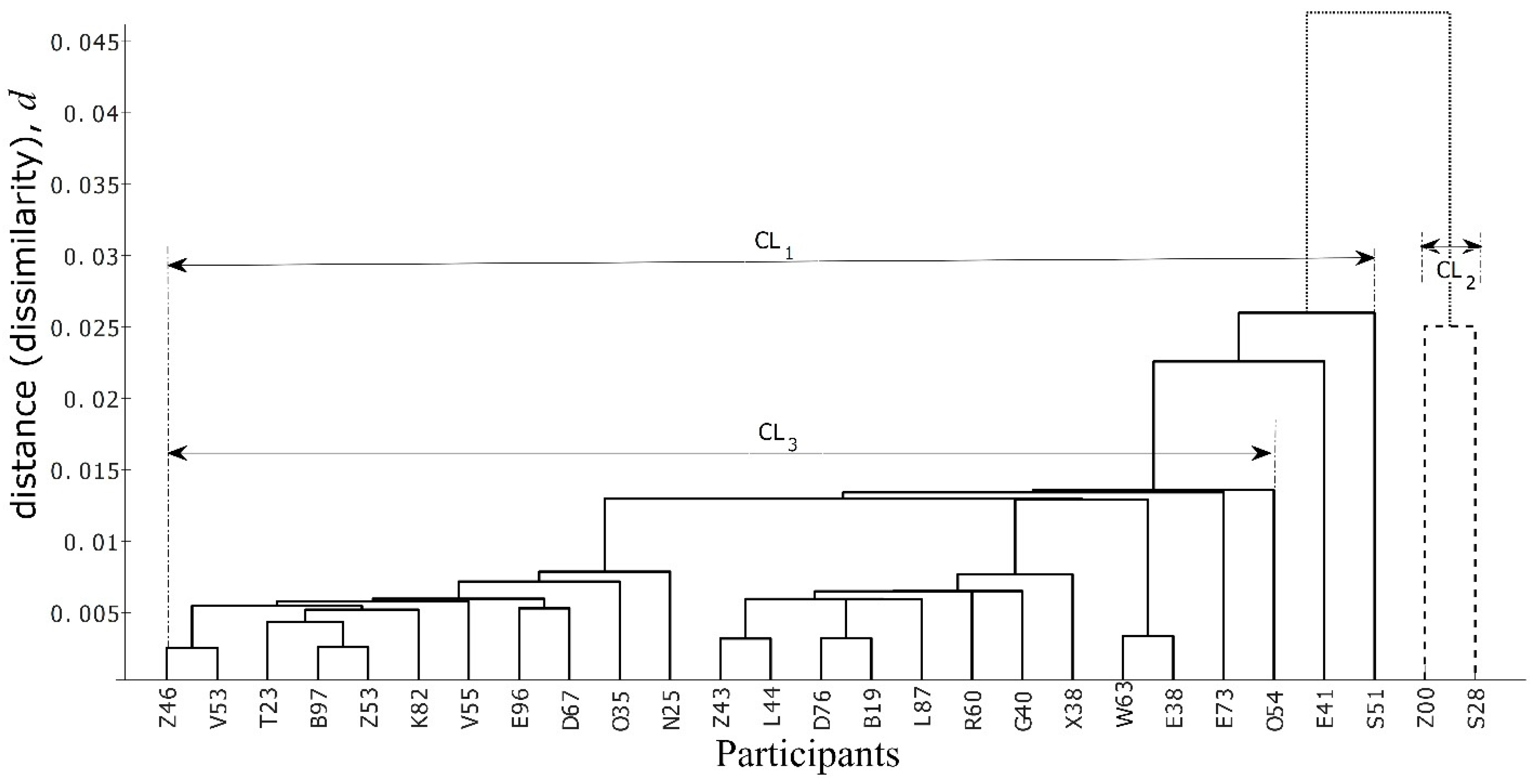
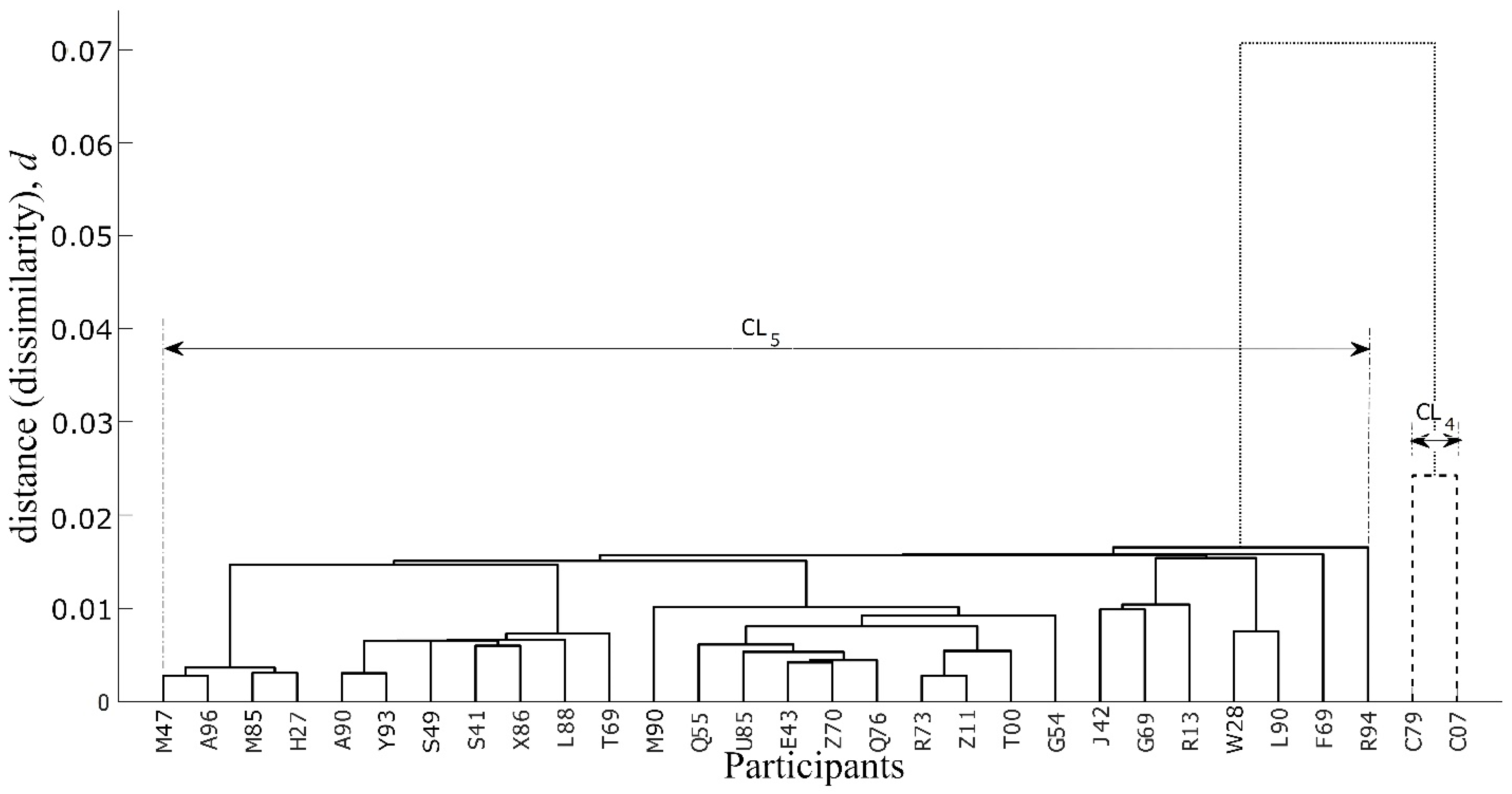
Structural similarity values among the graphs have been calculated per scenario. Because the graphs obtained in Section 5.7 have parallel edges between nodes, where each edge shows the activation of a function, the similarity between two graphs estimates the similarity in terms of the number of times respective functions, especially f1–f5, are performed. Figure 13 shows this functional similarity, i.e., the similarity among the graphs obtained by exploiting the number of times functions are repeated in FRAM data for Scenario 1, where mild ice conditions were observed. The similarity values for Scenario 2, which deals with clearing ice away from the lifeboat launch zone under severe ice conditions, are shown in Figure 14. Values outside the interval, where is the mean similarity of all participants and is the standard deviation, are quite evident (Figure 12 and Figure 13) and are considered as anomalies concerning the standard or majority behavior observed from the participants in both scenarios considered here. These values are obtained from four participants, two from each scenario. The participants’ code names for Scenario 1 (mild ice conditions) are Z00 and S28, and for Scenario 2 (severe ice conditions) are C79 and C07. The results obtained after similarity-based hierarchical clustering (Figure 14 and Figure 15) are also consistent with the direct similarity-based results (Figure 12 and Figure 13). That is, based on the values of the distance d (see Equation (3)), hierarchical clustering also suggested Z00, S28, C79, and C07 as showing anomalous behavior for the others performing the same tasks.
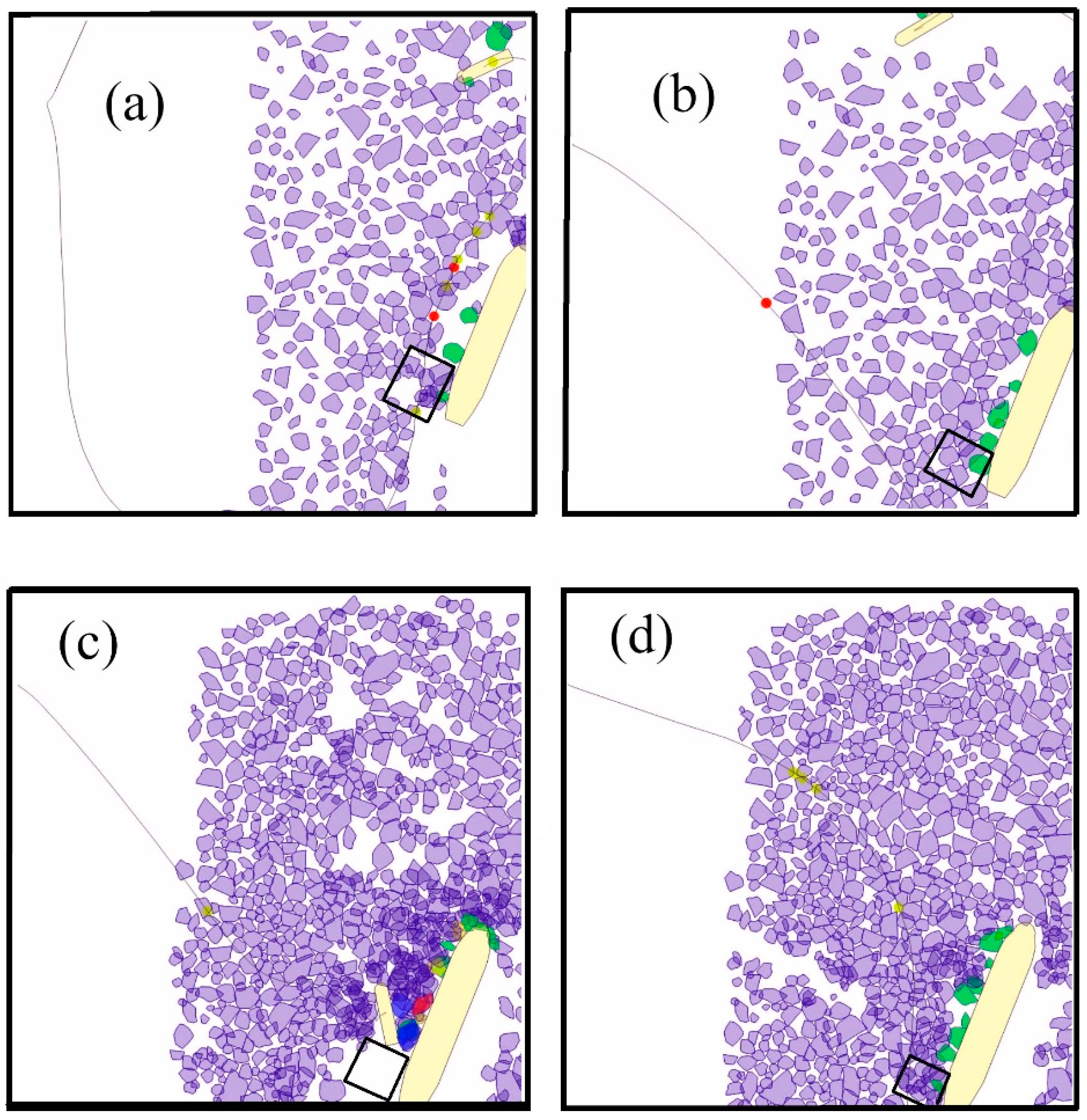
As shown in Figure 15, participants E41 and S51 are fused with the big cluster CL1 with rather higher distances almost equivalent to the height of the cluster CL2 that contains the participants Z00 and S28. This fusing is the result of the similarity (or low distance) between this group containing E41 and S51 and the cluster CL2, compared to the distance between the cluster CL2 and CL3 containing all the participants of CL1 excluding E41 and S51. This means that the performance of the cluster containing E41 and S51 should be considered as somewhat in the middle of the two clusters CL2 and CL3. This is also consistent with the empirical results (as shown in Table 2), where the clusters of Z00 and S28 are found to lie in the lower performance area in terms of “the total time lifeboat launch zone area is clear of ice” (LLTC). Participant S28 from the cluster CL2 had the lowest performance, as can be seen from Table 2, which shows the performance values based on the LLTC performance metric. However, the other member of the cluster CL2, i.e., Z00, does not lie immediately after S28 in Table 2, rather it is placed in the fourth place, having an LLTC value of 390. Even this value is on the lower side of the LLTC values, where the average is around 630. Similar findings can be observed in Figure 16a,b, which shows the area of the lifeboat launch zone rectangular region containing ice floes.
The case of Figure 17 that shows clustering for scenario 2 dealing with emergency ice management under severe ice conditions is clearer than that of the case presented in Figure 15. Here, the difference in the heights of the cluster CL4 containing the participants having code names C79 and C07 and the cluster CL5 containing all the other participants is large. This enables us to infer that C79 and C07 exploit a different pattern of activities embodied in the respective graphs, as shown in Figure 12. Again, this inference is supported by the empirical observations obtained in the respective experiment. That is, as shown in Table 2, the participant C79 is a high performing expert seafarer with extensive experience at sea. Based on the track chosen to approach the FPSO, participant C79 was amongst the top-performing participants in Scenario 2 [42] (p. 55). This is well supported in Figure 16c, where the area within the rectangular perimeters of the lifeboat launch zone water is clear of ice for almost 18 min out of the 30-min total duration of the scenario. The participant C07 was also a seafarer, but their performance remained on the lowest side. The replay video of C07 shows that the participant was unable to clear ice from the lifeboat launch zone as was required in the task (see Figure 16d).
7. Conclusions
The methodology developed here shows the potential to detect anomalies in human performance data presented in the form of FRAM instantiations. The question of whether the anomaly is caused by an expert behavior or is due to an error, which may indicate a lack of experience or training of personnel, can be answered by exploiting the approach developed here. This means that the proposed approach has the potential to discover unusual behavior from the given datasets of human performance data presented in the form of FRAM instantiations, which is difficult to find out by exploiting conventional statistical techniques. For example, the detection of the pattern of activities by the participants C79 and C07 as described in the preceding section is an important result that came up by examining the difference in the clusters shown in Figure 16. To this point, the quantification of the unusual behavior is possible from the proposed technique, but hereafter, the proposed approach relies on reading the experimental results to find out the cause of the detected unusual or anomalous behavior. The authors think that a more detailed quantification is possible if functional accuracies are available in the FRAM data, that is, if it is known which function was performed correctly and to what extent. In practice, there are limitations to practically estimating minute differences in functional outputs, especially in complex socio-technical systems such as the case studies presented here. For example, instead of using a Boolean value that a function has been performed or not performed, a value, say x percent, of the tasks associated by the complete execution of the function f has been performed is more important than the absolute value of the functional output, such as the speed in knots, because FRAM based modeling involves functional aspects and performance variability rather than physical aspects [49]. The present approach may be supplemented with an approach to accommodate the functional accuracies to suggest at what point in time the activity of a participant turns to an anomaly.
Author Contributions
Onceptualization, S.N.D., D.S., and B.V.; methodology, S.N.D.; software, S.N.D.; validation, S.N.D., and D.S.; formal analysis, S.N.D.; investigation, S.N.D.; resources, D.S. and B.V.; data curation, S.N.D., D.S., and B.V.; writing—original draft preparation, S.N.D.; writing—review and editing, S.N.D. and D.S.; visualization, S.N.D.; supervision, S.N.D.; project administration, B.V.; funding acquisition, B.V. All authors have read and agreed to the published version of the manuscript.
Funding
NSERC/Husky Energy Industrial Research Funding.
Institutional Review Board Statement
The study was conducted according to the guidelines of the Declaration of Memorial University of Newfoundland, and approved by the ICEHR–Application for Ethics Review (Secondary Use of Data) of Memorial University of Newfoundland, NL, Canada (File Number 20201600 and approved on 11 February 2020).
Informed Consent Statement
Not applicable.
Data Availability Statement
The data presented in this study are available on request from the corresponding author. The data are not publicly available due to privacy of human subjects used in this study.
Acknowledgments
The authors acknowledge with gratitude the support of the NSERC/Husky Energy Industrial Research Chair in Safety at Sea.
Conflicts of Interest
The authors declare no conflict of interest.
References
- Hollnagel, E. FRAM: The Functional Resonance Analysis Method: Modelling Complex Socio-Technical Systems, 1st ed.; CRC Press: Surrey, UK, 2012. [Google Scholar]
- Hollnagel, E. Safety-I and Safety-II: The Past and Future of Safety Management, 1st ed.; CRC Press: Boca Raton, FL, USA, 2014. [Google Scholar]
- Smith, D.; Veitch, B.; Khan, F.; Taylor, R. Integration of Resilience and FRAM for Safety Management. ASCE-ASME J. Risk Uncertain. Eng. Syst. Part A Civ. Eng. 2020, 6, 04020008. [Google Scholar] [CrossRef]
- Ayyub, B.M. Practical Resilience Metrics for Planning, Design, and Decision Making. ASCE-ASME J. Risk Uncertain. Eng. Syst. Part A Civ. Eng. 2015, 1, 04015008. [Google Scholar] [CrossRef]
- Hodge, V.; Austin, J. A Survey of Outlier Detection Methodologies. Artif. Intell. Rev. 2004, 22, 85–126. [Google Scholar] [CrossRef] [Green Version]
- Krousel-Wood, M.A.; Chambers, R.B.; Muntner, P. Clinicians’ Guide to Statistics for Medical Practice and Research: Part I. Ochsner J. 2006, 6, 68–83. [Google Scholar] [PubMed]
- Theodoridis, S.; Koutroumbas, K. Pattern Recognition; Academic Press: San Diego, CA, USA, 1999. [Google Scholar]
- Wills, P.; Meyer, F.G. Metrics for Graph Comparison: A Practitioner’s Guide. PLoS ONE 2020, 15, e0228728. [Google Scholar] [CrossRef] [Green Version]
- Lewis, T.G. Network Science: Theory and Applications; John Wiley & Sons Inc.: Hoboken, NJ, USA, 2009. [Google Scholar]
- Borgatti, S.P.; Everett, M.G.; Johnson, J.C. Analyzing Social Networks; SAGE Publications Ltd.: Los Angeles, CA, USA, 2013. [Google Scholar]
- Neal, Z.P. A Sign of the Times? Weak and Strong Polarization in the U.S. Congress, 1973–2016. Soc. Netw. 2020, 60, 103–112. [Google Scholar] [CrossRef]
- Bunke, H.; Allermann, G. Inexact Graph Matching for Structural Pattern Recognition. Pattern Recognit. Lett. 1983, 1, 245–253. [Google Scholar] [CrossRef]
- Vento, M. A Long Trip in the Charming World of Graphs for Pattern Recognition. Pattern Recognit. 2015, 48, 291–301. [Google Scholar] [CrossRef]
- Conte, D.; Foggia, P.; Sansone, C.; Vento, M. Thirty Years of Graph Matching in Pattern Recognition. Int. J. Pattern Recognit. Artif. Intell. 2004, 18, 265–298. [Google Scholar] [CrossRef]
- Caetano, T.S.; McAuley, J.J.; Li, C.; Le, Q.V.; Smola, A.J. Learning Graph Matching. IEEE Trans. Pattern Anal. Mach. Intell. 2009, 31, 1048–1058. [Google Scholar] [CrossRef] [Green Version]
- Bunke, H.; Foggia, P.; Guidobaldi, C.; Vento, M. Graph clustering using the weighted minimum common supergraph. In Lecture Notes in Computer Science (including subseries Lecture Notes in Artificial Intelligence and Lecture Notes in Bioinformatics); Springer: Berlin, German, 2003; Volume 2726, pp. 235–246. [Google Scholar]
- Foggia, P.; Percannella, G.; Sansone, C.; Vento, M. A Graph-Based Clustering Method and Its Applications. Lect. Notes Comput. Sci. (Subser. Lect. Notes Artif. Intell. Lect. Notes Bioinform.) 2007, 4729 LNCS, 277–287. [Google Scholar] [CrossRef]
- Cheng, H.D.; Cai, X.; Chen, X.; Hu, L.; Lou, X. Computer-Aided Detection and Classification of Microcalcifications in Mammograms: A Survey. Pattern Recognit. 2003, 36, 2967–2991. [Google Scholar] [CrossRef]
- Rokach, L.; Maimon, O. Clustering Methods. In Data Mining and Knowledge Discovery Handbook; Springer: New York, NY, USA, 2006; pp. 321–352. [Google Scholar]
- Schaeffer, S.E. Graph Clustering. Comput. Sci. Rev. 2007, 1, 27–64. [Google Scholar] [CrossRef]
- Malliaros, F.D.; Vazirgiannis, M. Clustering and Community Detection in Directed Networks: A Survey. Phys. Rep. 2013, 533, 95–142. [Google Scholar] [CrossRef] [Green Version]
- Loe, C.W.; Jensen, H.J. Comparison of Communities Detection Algorithms for Multiplex. Phys. A Stat. Mech. Appl. 2015, 431, 29–45. [Google Scholar] [CrossRef] [Green Version]
- Saxena, A.; Prasad, M.; Gupta, A.; Bharill, N.; Patel, O.P.; Tiwari, A.; Er, M.J.; Ding, W.; Lin, C.-T. A Review of Clustering Techniques and Developments. Neurocomputing 2017, 267, 664–681. [Google Scholar] [CrossRef] [Green Version]
- Farag, A.; Abdelkader, H.; Salem, R. Parallel Graph-Based Anomaly Detection Technique for Sequential Data. J. King Saud Univ. Comput. Inf. Sci. 2019. [Google Scholar] [CrossRef]
- Pourhabibi, T.; Ong, K.-L.; Kam, B.H.; Boo, Y.L. Fraud Detection: A Systematic Literature Review of Graph-Based Anomaly Detection Approaches. Decis. Support Syst. 2020, 133, 113303. [Google Scholar] [CrossRef]
- Prado-Romero, M.A.; Gago-Alonso, A. Community feature selection for anomaly detection in attributed graphs. In Lecture Notes in Computer Science (Subser. Lect. Notes Artif. Intell. Lect. Notes Bioinform.); Lecture Notes in Computer Science; Beltrán-Castañón, C., Nyström, I., Famili, F., Eds.; Springer International Publishing: Cham, Switzerland, 2017; Volume 10125 LNCS, pp. 109–116. ISBN 9783319522760. [Google Scholar]
- Papadimitriou, P.; Dasdan, A.; Garcia-Molina, H. Web Graph Similarity for Anomaly Detection. J. Internet Serv. Appl. 2010, 1, 19–30. [Google Scholar] [CrossRef] [Green Version]
- Patriarca, R.; Bergström, J.; Di Gravio, G. Defining the Functional Resonance Analysis Space: Combining Abstraction Hierarchy and FRAM. Reliab. Eng. Syst. Saf. 2017, 165, 34–46. [Google Scholar] [CrossRef]
- Rasmussen, J. The Role of Hierarchical Knowledge Representation in Decisionmaking and System Management. IEEE Trans. Syst. Man. Cybern. 1985, SMC-15, 234–243. [Google Scholar] [CrossRef]
- Duan, G.; Tian, J.; Wu, J. Extended FRAM by Integrating with Model Checking to Effectively Explore Hazard Evolution. Math. Probl. Eng. 2015, 2015, 1–11. [Google Scholar] [CrossRef] [Green Version]
- Patriarca, R.; Di Gravio, G.; Woltjer, R.; Costantino, F.; Praetorius, G.; Ferreira, P.; Hollnagel, E. Framing the FRAM: A Literature Review on the Functional Resonance Analysis Method. Saf. Sci. 2020, 129, 104827. [Google Scholar] [CrossRef]
- Moher, D.; Liberati, A.; Tetzlaff, J.; Altman, D.G. Preferred Reporting Items for Systematic Reviews and Meta-Analyses: The PRISMA Statement. PLoS Med. 2009, 6, e1000097. [Google Scholar] [CrossRef] [Green Version]
- Falegnami, A.; Costantino, F.; Di Gravio, G.; Patriarca, R. Unveil Key Functions in Socio-Technical Systems: Mapping FRAM into a Multilayer Network. Cogn. Technol. Work 2020, 22, 877–899. [Google Scholar] [CrossRef]
- Yu, M.; Quddus, N.; Kravaris, C.; Mannan, M.S. Development of a FRAM-Based Framework to Identify Hazards in a Complex System. J. Loss Prev. Process Ind. 2020, 63. [Google Scholar] [CrossRef]
- Bicego, M.; Murino, V.; Pelillo, M.; Torsello, A. Similarity-Based Pattern Recognition. Pattern Recognit. 2006, 39, 1813–1814. [Google Scholar] [CrossRef]
- Hartsfield, N.; Ringel, G. Pearls in Graph Theory: A Comprehnsive Introduction; Academic Press, Inc.: Boston, MA, USA, 1990. [Google Scholar]
- Koutra, D.; Shah, N.; Vogelstein, J.T.; Gallagher, B.; Faloutsos, C. DELTACON: Principled Massive-Graph Similarity Function with Attribution. ACM Trans. Knowl. Discov. Data 2016, 10, 1–43. [Google Scholar] [CrossRef]
- Hollnagel, E. FRAM: The Functional Resonance Analysis Method. 2018. Available online: https://functionalresonance.com/onewebmedia/Manualds1.docx.pdf (accessed on 16 February 2021).
- Haji, F.A.; Cheung, J.J.H.; Woods, N.; Regehr, G.; de Ribaupierre, S.; Dubrowski, A. Thrive or Overload? The Effect of Task Complexity on Novices’ Simulation-Based Learning. Med. Educ. 2016, 50, 955–968. [Google Scholar] [CrossRef] [PubMed]
- Tichon, J.G.; Wallis, G.M. Stress Training and Simulator Complexity: Why Sometimes More Is Less. Behav. Inf. Technol. 2010, 29, 459–466. [Google Scholar] [CrossRef]
- Veitch, E.; Molyneux, D.; Smith, J.; Veitch, B. Investigating the Influence of Bridge Officer Experience on Ice Management Effectiveness Using a Marine Simulator Experiment. J. Offshore Mech. Arct. Eng. 2019, 141. [Google Scholar] [CrossRef] [Green Version]
- Veitch, E. Influence of Bridge Officer Experience on Ice Management Effectiveness. Master’s Thesis, Memorial University of Newfoundland, St. John’s, NL, Canada, 2018. [Google Scholar]
- Thistle, R. Evaluation of the Effects of Simulator Training on Ice Management Performance. Ph.D. Thesis, Memorial University of Newfoundland, St. John’s, NL, Canada, 2019. [Google Scholar]
- Thistle, R.; Veitch, B. An Evidence-Based Method of Training to Targeted Levels of Performance. In Proceedings of the 2019 SNAME Maritime Convention, Tacoma, WA, USA, 30 October–1 November Tacoma; The Society of Naval Architects and Marine Engineers: Tacoma, WA, USA, 2019. [Google Scholar]
- IMO. International Code for Ships Operating in Polar Waters (Polar Code); International Maritime Organization: London, UK, 2017; Volume MEPC. [Google Scholar]
- IMO. Guidance on Methodologies for Assessing Operational Capabilities and Limitations in Ice; MSC.1/Circ. 1519; International Maritime Organization: London, UK, 2016. [Google Scholar]
- Smith, D.; Veitch, E.; Veitch, B.; Khan, F.; Taylor, R. Visualizing and Understanding the Operational Dynamics of a Shipping Operation. In Proceedings of the SNAME Maritime Convention, Providence, RI, USA, 24 October 2018; The Society of Naval Architects and Marine Engineers (SNAME): Providence, RI, USA, 2018. [Google Scholar]
- Smith, D.; Veitch, B.; Khan, F.; Taylor, R. Using the FRAM to Understand Arctic Ship Navigation: Assessing Work Processes During the Exxon Valdez Grounding. TransNav Int. J. Mar. Navig. Saf. Sea Transp. 2018, 12, 447–457. [Google Scholar] [CrossRef]
- Salehi, V.; Smith, D.; Veitch, B. Modeling Complex Socio-technical Systems Using the FRAM: A Literature Review. Hum. Factors Ergon. Manuf. Serv. Ind. 2021, 31, 118–142. [Google Scholar] [CrossRef]
Figure 1.
A method to use structural similarity-based clustering for analyzing anomalies in FRAM-models.
Figure 1.
A method to use structural similarity-based clustering for analyzing anomalies in FRAM-models.

Figure 2.
The process of making a FRAM model and recording the instantiations.

Figure 3.
An example of a FRAM instantiation. Functions f1–f7 are part of the FRAM model for which the instantiation takes three rounds/cycles. For a better visibility, each cycle is represented in a different line style (cycle 1: solid line; cycle 2: dashed line; and cycle 3: dotted line). Note there are six aspects for each FRAM node: T represents the aspect time, C shows control, I is for input, O is for output, P represents preconditions, and R is used to show any resources that are required by the function.

Figure 4.
The graph obtained after applying Algorithm 1 on the example FRAM instantiation of Figure 3. The parallel edges show the likelihood of functional resonance and can be stored as the weight of a single edge.
Figure 4.
The graph obtained after applying Algorithm 1 on the example FRAM instantiation of Figure 3. The parallel edges show the likelihood of functional resonance and can be stored as the weight of a single edge.

Figure 5.
A method to detect anomalies in human performance data expressed as FRAM.

Figure 6.
Schematics of ice management simulator used in Experiments 1 and 2.

Figure 7.
Bridge simulator schematics.

Figure 8.
The FRAM model to represent participant’s performance in Experiments 1 and 2.

Figure 9.
A portion of FRAM instantiation (first 93 s of 30 min) obtained after applying the FRAM model of Figure 8 on a participant with code name S51 performing emergency ice management scenario with mild ice conditions. The dashed lines only show repetition of previous activities. In other words, the dashed lines are used to show the cyclic nature of the ice-management activity.

Figure 10.
A participant from group G1 performing the emergency ice management scenario in mild ice conditions (4 tenths concentration).
Figure 10.
A participant from group G1 performing the emergency ice management scenario in mild ice conditions (4 tenths concentration).

Figure 11.
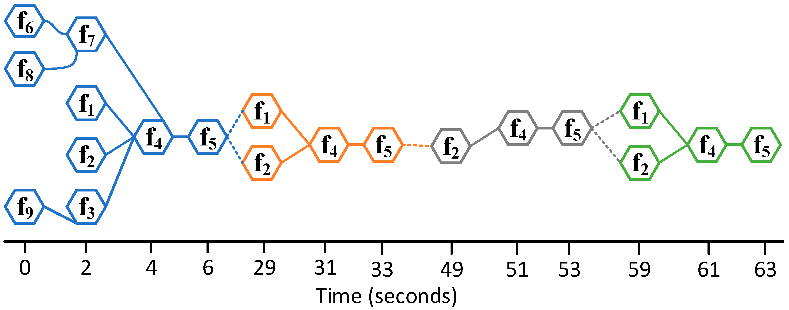
A portion of FRAM instantiation (first 63 s of 30 min) obtained after applying the FRAM model of Figure 8 on a participant with code name Y42 performing the emergency ice management scenario with severe ice conditions. The dashed lines only show the repetition of previous activities. In other words, the dashed lines are used to show the cyclic nature of the ice-management activity.
Figure 11.
A portion of FRAM instantiation (first 63 s of 30 min) obtained after applying the FRAM model of Figure 8 on a participant with code name Y42 performing the emergency ice management scenario with severe ice conditions. The dashed lines only show the repetition of previous activities. In other words, the dashed lines are used to show the cyclic nature of the ice-management activity.

Figure 12.
Sections of the graphs obtained after applying Algorithm 1 on the FRAM instantiations of four participants. The circles show the nodes of the graphs. Parallel edges are evident that show each function being activated repeatedly in the respective scenarios. (a) A graph obtained from the participant with code name C79 performing Scenario 2, (b) graph for the participant with code name C07 performing Scenario 2, (c) graph for the participant with code name S51 performing Scenario 1, and (d) graph for the participant with code name V55 performing Scenario 1.

Figure 13.
Comparison of participants (code names on the x-axis) based on similarity values. Each value represents how similar a participant’s performance has been concerning the average performance of all the participants in mild ice conditions, i.e., Scenario 1. The similarity values corresponding to the participants with code names Z00 and S28 are well outside the interval (shown as dotted horizontal lines), where is the mean similarity of all participants and is the standard deviation.

Figure 14.
Comparison of participants based on similarity values. Each value represents how similar a participant’s performance has been for the overall performance of all the participants in severe ice conditions, i.e., Scenario 2. The similarity values corresponding to the participants with code names C79 and C07 are well outside the interval (shown as dotted horizontal lines), where is the mean similarity of all participants and is the standard deviation.

Figure 15.
Similarity-based hierarchical clustering (a dendrogram) of graphs obtained from mild ice emergency scenario. Participants Z00 and S28 are similar to each other in performance (the cluster with the dashed lines) and are different from the cluster CL1, as is visible through the difference in heights of both clusters.

Figure 16.
The snapshots taken at the 20th minute of the 30-min replay videos during emergency evacuation scenarios in mild (a,b) and severe ice conditions (c,d). The rectangular regions in all four snaps show an approximate location of the lifeboat launch zone. The lower the amount of ice floes in the rectangular region near the portside of the vessel’s stern in (a–d), the higher the performance. (a) Performance of participant Z00 in Scenario 1, (b) performance of participant S28 in Scenario 1, (c) performance of participant C79 in Scenario 2, and (d) performance of participant C07 in Scenario 2.

Figure 17.
Similarity-based hierarchical clustering of graphs obtained from severe ice emergency scenario. Participants with code names C79 and C07 are similar to each other in performance (the cluster with dotted lines) and are markedly different from the big cluster (solid lines), as is visible through the difference in heights of both clusters.


Table 1.
Mapping of participants’ activities during emergency ice management scenario to the respective function. The data below shows activities performed by the participant S51 during the emergency ice management scenario. Each distinct activity is considered as a function, called active function. The downstream function is the one that will follow the active function stops its execution. The aspect of downstream function that will carry the result or data from the active function is represented below as the last column. Note: Only a few initial aspects involve anything but the aspect I.
| Time (s) | Activity | Active Function | Downstream Function | Aspect of Function |
|---|---|---|---|---|
| 0 | Getting vessel class, Class 1C | f8 | f7 | P |
| 0 | Getting ice type information | f6 | f7 | I |
| 0 | Checking speed limit, speed < 3 knot | f9 | f3 | P |
| 2 | Get heading and speed | f3 | f4 | I |
| 2 | Get ice concentration in zone | f1 | f4 | I |
| 2 | Get vessel location | f2 | f4 | I |
| 4 | Complete or partial assessment of situation | f4 | f5 | I |
| 6 | Update ice condition, vessel location, speed update | f5 | f1 | I |
| 6 | Update ice condition, vessel location, speed update | f5 | f2 | I |
| 29 | Get ice concentration in zone | f1 | f4 | I |
| 29 | Get vessel location | f2 | f4 | I |
| 31 | Complete or partial assessment of situation | f4 | f5 | I |
| 33 | Update ice condition, vessel location, speed update | f5 | f1 | I |
| 33 | Update ice condition, vessel location, speed update | f5 | f2 | I |
| 59 | Get ice concentration in zone | f1 | f4 | I |
| 59 | Get vessel location | f2 | f4 | I |
| 61 | Complete or partial assessment of situation | f4 | f5 | I |
| 63 | Update ice condition, vessel location, speed update | f5 | f1 | I |
| 63 | Update ice condition, vessel location, speed update | f5 | f2 | I |
| 63 | Update ice condition, vessel location, speed update | f5 | f3 | I |
| 89 | Get ice concentration in zone | f1 | f4 | I |
| 89 | Get vessel location | f2 | f4 | I |
| 89 | Get heading and speed | f3 | f4 | I |
| 91 | Complete or partial assessment of situation | f4 | f5 | I |
| 93 | Update ice condition, vessel location, speed update | f5 | f1 | I |
| 93 | Update ice condition, vessel location, speed update | f5 | f2 | I |
| 119 | Get ice concentration in zone | f1 | f4 | I |
Table 2.
The total time lifeboat launch zone is clear of ice, which is the performance metric that measures the maximum total consecutive time during the 30-min ice management scenario that the lifeboat launch zone is clear of ice and is considered ready for lifeboat launch in case of an emergency.
Table 2.
The total time lifeboat launch zone is clear of ice, which is the performance metric that measures the maximum total consecutive time during the 30-min ice management scenario that the lifeboat launch zone is clear of ice and is considered ready for lifeboat launch in case of an emergency.
| Participant | Scenario | LTTC (s) | Participant | Scenario | LTTC (s) |
|---|---|---|---|---|---|
| S28 | 1 | 20 | J42 | 2 | 0 |
| W63 | 1 | 80 | S41 | 2 | 20 |
| E73 | 1 | 320 | C07 | 2 | 50 |
| Z00 | 1 | 390 | R94 | 2 | 130 |
| Z46 | 1 | 390 | T00 | 2 | 150 |
| G40 | 1 | 400 | W28 | 2 | 270 |
| Z53 | 1 | 400 | S49 | 2 | 280 |
| Z43 | 1 | 460 | T69 | 2 | 340 |
| R60 | 1 | 470 | G54 | 2 | 340 |
| T23 | 1 | 480 | M47 | 2 | 390 |
| S51 | 1 | 530 | R13 | 2 | 430 |
| V53 | 1 | 530 | Z11 | 2 | 430 |
| L87 | 1 | 610 | L96 | 2 | 490 |
| E38 | 1 | 610 | E43 | 2 | 500 |
| B19 | 1 | 680 | U85 | 2 | 520 |
| B97 | 1 | 680 | O07 | 2 | 540 |
| D67 | 1 | 700 | H27 | 2 | 550 |
| D76 | 1 | 700 | Y42 | 2 | 570 |
| E96 | 1 | 720 | M90 | 2 | 590 |
| V55 | 1 | 730 | F69 | 2 | 650 |
| E41 | 1 | 830 | A96 | 2 | 730 |
| O54 | 1 | 840 | Q76 | 2 | 760 |
| X38 | 1 | 900 | L90 | 2 | 780 |
| O35 | 1 | 960 | X86 | 2 | 820 |
| K82 | 1 | 980 | L88 | 2 | 880 |
| L44 | 1 | 1230 | Q55 | 2 | 910 |
| N25 | 1 | 1350 | Z70 | 2 | 940 |
| M85 | 2 | 960 | |||
| Y93 | 2 | 1010 | |||
| A90 | 2 | 1020 | |||
| C79 | 2 | 1090 | |||
| G69 | 2 | 1120 | |||
| N08 | 2 | 1140 | |||
| R73 | 2 | 1150 |
Publisher’s Note: MDPI stays neutral with regard to jurisdictional claims in published maps and institutional affiliations. |
© 2021 by the authors. Licensee MDPI, Basel, Switzerland. This article is an open access article distributed under the terms and conditions of the Creative Commons Attribution (CC BY) license (http://creativecommons.org/licenses/by/4.0/).
Share and Cite
MDPI and ACS Style
Danial, S.N.; Smith, D.; Veitch, B. A Method to Detect Anomalies in Complex Socio-Technical Operations Using Structural Similarity. J. Mar. Sci. Eng. 2021, 9, 212. https://0-doi-org.brum.beds.ac.uk/10.3390/jmse9020212
AMA Style
Danial SN, Smith D, Veitch B. A Method to Detect Anomalies in Complex Socio-Technical Operations Using Structural Similarity. Journal of Marine Science and Engineering. 2021; 9(2):212. https://0-doi-org.brum.beds.ac.uk/10.3390/jmse9020212
Chicago/Turabian StyleDanial, Syed Nasir, Doug Smith, and Brian Veitch. 2021. "A Method to Detect Anomalies in Complex Socio-Technical Operations Using Structural Similarity" Journal of Marine Science and Engineering 9, no. 2: 212. https://0-doi-org.brum.beds.ac.uk/10.3390/jmse9020212
Note that from the first issue of 2016, this journal uses article numbers instead of page numbers. See further details here.