The Response of the Water Surface Layer to Internal Turbulence and Surface Forcing

Abstract

We have carried out an experimental study of the turbulence kinetic energy dissipation rate ($ϵ$), temperature dissipation rate ($\chi$), and turbulent heat flux (THF) within the water surface layer in the presence of non-breaking wave, surface convection, and horizontal heat and eddy fluxes that play a prominent role in the front. We noted that the non-breaking wave dominates $ϵ$ values within the surface layer. While analyzing the vertical $ϵ$ variability, the presence of a wave-affected layer from the water surface to a depth of $z\approx 1.25{\lambda }_{\mathrm{w}}$ is observed, where ${\lambda }_{\mathrm{w}}$ is the wavelength. $ϵ$ associated with non-breaking waves ranged to $4.9\times {10}^{-6}$–$7\times {10}^{-6}$ m²/s³ for the wavelength range of 0.038 m < ${\lambda }_{\mathrm{w}}$ < 0.098 m categorized as the gravity and gravity-capillary wave regimes. $ϵ$ values increase for longer ${\lambda }_{\mathrm{w}}$ and non-breaking wave $ϵ$ values represent their significant contribution to the ocean energy budget and dynamic of surface layer considering that the non-breaking wave covers the large fraction of ocean surface. We also found that the surface mean square slope (MSS) and wave generated $ϵ$ have the same order of magnitude, i.e., MSS $\sim ϵ$. Besides, we have documented that the small-scale temperature fluctuation change (i.e., $\chi$) is consistent with the large-scale temperature gradient change (i.e., $d<T>/dz$). The value of the THF is approximately constant within the surface layer. It represents that the measured THF near the water surface can be considered a surface water THF, challenging to measure directly.

1. Introduction

The ocean covers approximately 71 percent of the Earth’s surface [1]. At the air–sea interface, the exchange of heat, moisture, momentum, and gas transfer is carried out by molecular transfer processes; however, at a depth greater than ∼1 mm, the turbulence dominates the mixing processes [2]. $ϵ$ value has implications on heat flux across the ocean interface [3], the air–sea gas fluxes velocity, $K_g\sim {ϵ}^{1/4}$ [4] and it is essential for the oil industry [5] due to that the higher turbulence enhances the biodegradation of oil [6]. Understanding $ϵ$ distribution and its role in near-surface water and ocean mixing are vital in studying ocean processes and the upper ocean boundary layer dynamic.

The value of $ϵ$ can be then found from the relationship $ϵ=2\upsilon <s_{ij}{s}_{ij}>$ [7], where $s_{ij}$ is the fluctuating rate of strain: $s_{ij}=\frac{1}{2}(\frac{\partial u_i^{\prime }}{\partial x_j}+\frac{\partial u_j^{\prime }}{\partial x_i})$. Here, $\upsilon$ is the kinematic molecular viscosity, i and j = 1, 2, and 3, and correspond to x, y and z coordinates, respectively. $u_i^{\prime }$ represents the fluctuating part of the velocity components, and <> is the ensemble average. The value of $\chi$ comes from the equation $\chi =2K_{\theta }<{\left(\frac{\partial \theta }{\partial x_i}\right)}^2>=2K_{\theta }<{\left(\frac{\partial \theta }{\partial x}\right)}^2+{\left(\frac{\partial \theta }{\partial y}\right)}^2+{\left(\frac{\partial \theta }{\partial z}\right)}^2>$, where $K_{\theta }$ is the thermal molecular diffusivity, and $\theta$ is the fluctuating part of temperature. The vertical $ϵ$ and $\chi$ variability have been investigated within the upper ocean boundary layer while the boundary layer is influenced by one of the surface forcing such as heat flux [4,8], internal sources of turbulence [9], surface gravity wave [8,10,11,12,13], and capillary wave [14]. Fredriksson et al. [4] simulated a numerical model to calculate $ϵ$ for a free surface flow driven by natural convection. They found that the oceanic free convection results in a sharp change of $ϵ$ beneath the water surface. Wuest et al. [15] measured $ϵ$ in the wind-forced stratified water and observed that ≈90% of turbulent kinetic energy was dissipated within the upper boundary layer. Terray et al. [16] investigated $ϵ$ under breaking waves and observed a large uniform $ϵ$ from the surface water to a depth of $z=0.6H_s$, where $H_s$ is the significant wave height.

Given that the percentage of the ocean surface covered by wave breaking under strong wind is less than 10% [17], it indicates the significant role of the non-breaking wave on the ocean budget. Babanin and Haus [18] conducted a laboratory experiment to measure $ϵ$ beneath monochromatic non-breaking waves, which showed the presence of $ϵ$. Bogucki et al. [19] observed that $ϵ$ associated with non-breaking solitary waves ranged to $3\times {10}^{-4}$ m${}^2$/s${}^3$ for a wave amplitude of 50 cm.

The scarcity of field data hinders $ϵ$ and $\chi$ universal parametrization within the upper ocean boundary layer, especially very near the surface. This paper presents laboratory experiments in the Air–Sea Interaction Saltwater Tank (ASIST) at the University of Miami. We try to simply simulate the ocean when the horizontal heat and eddy fluxes play a prominent role in the ocean, like the front in the Gulf of Mexico where the Mississippi River with massive horizontal eddy fluxes reach the ocean and generate the Front [13,20]. We investigate the THF, $\chi$, and $ϵ$ variability very close to the air–sea interface, 0.5 cm beneath the water surface, when subject to the internal turbulence, surface convection, and non-breaking wave categorized as the gravity and gravity-capillary wave regimes [21,22,23]. The sources of turbulence and temperature flux in our experiment and the experimental setup are addressed in Section 2. Section 3 describes the experimental results of $ϵ$, $\chi$, and THF. Finally, a conclusion is given in Section 4.

2. Experimental Setup, Data Acquisition, and Analysis

We simulated the oceanic-like forcing in our laboratory experiment by having the three turbulence sources, i.e., the internal sources of turbulence, surface convection, and non-breaking surface waves.

2.1. Experimental Setup

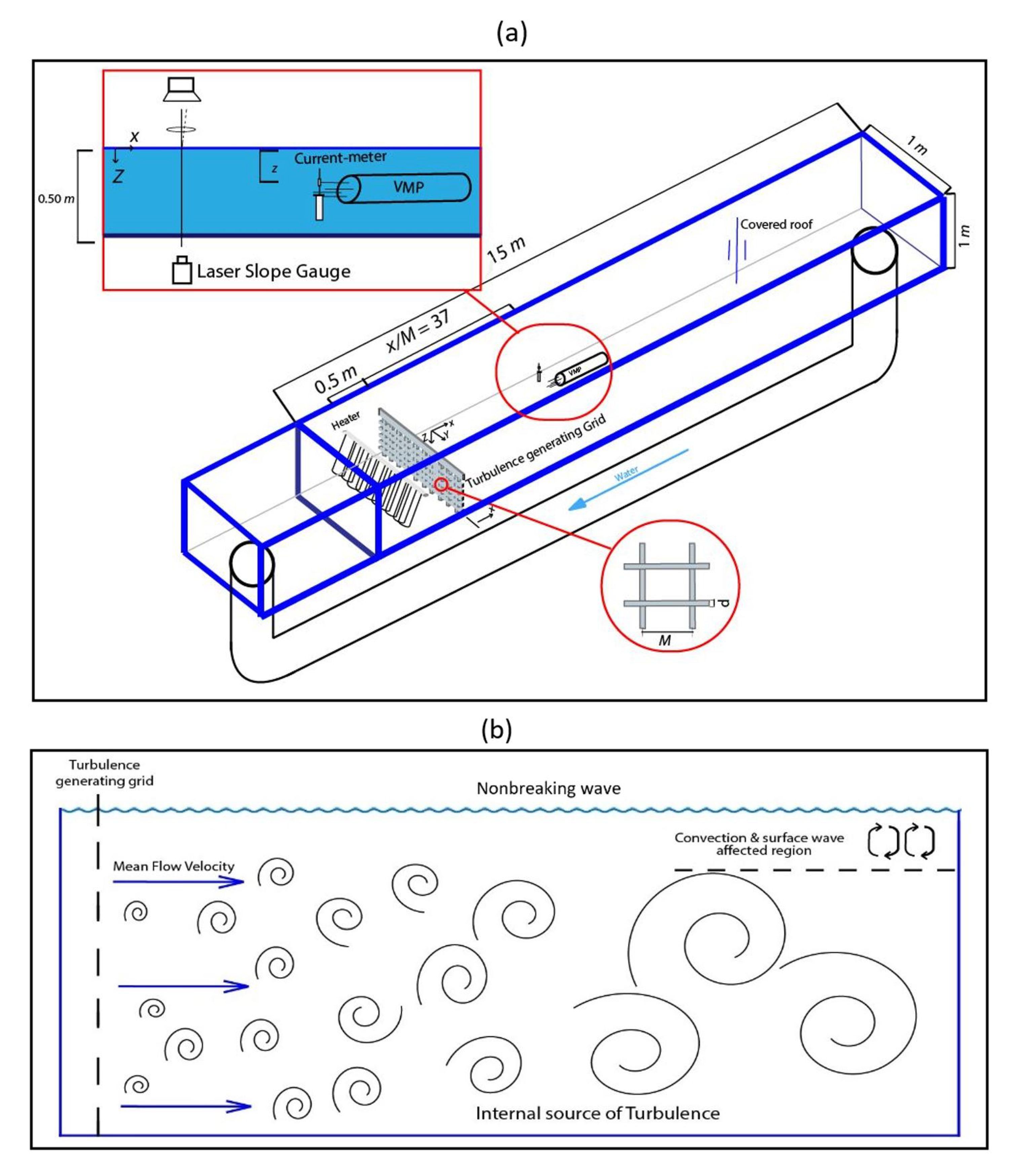
The experiments were conducted in the ASIST tank at the University of Miami, equipped with the turbulence generating grid and a heated grid (Figure 1). The tank walls are constructed of acrylic panels with a thickness of $0.024$ m and have dimensions 15 m long, 1 m wide, and 1 m high. In our experiment, we analyzed data for the mean water flow velocity of $<U>=0.066$ m/s, 0.125 m/s, 0.167 m/s, and 0.183 m/s. The heated grid was located at the tank entrance, and the turbulence-generating grid was mounted $0.5$ m behind the heater. The freshwater depth during the experiment was kept constant, $d_t=$ $0.5$ m. The thickness of the bar of the grid was $d_b=0.02$ m, and the distance between the centers of two cells on the grid horizontally and vertically was $M=0.1$ m. The solidity of the grid was $\sigma =\frac{d_b}{M}(2-\frac{d_b}{M})=0.36$ [24]. The grid Reynolds number in our experiment was given by $R{e}_M=(\sigma M<U>/\upsilon )$ [25] (

Table 1. The table indicates the summary of the experiment.

<U> = Mean Flow Velocity (m/s)	0.101	0.125	0.167	0.183
$R{e}_M$ = ($\sigma$ M <U>/$\upsilon$) = grid Reynolds number	2366	4482	5988	6630
MSS = Mean square slope	$2.35\times {10}^{-5}$	$6.2\times {10}^{-5}$	$1.04\times {10}^{-4}$	$1.23\times {10}^{-4}$
${\lambda }_{\mathrm{w}}=$ wavelength (m)	0.038	0.051	0.074	0.098
H = $2<\eta >$ = wave height (m)	0.003	0.0034	0.0060	0.0068
${ϵ}_0$ = background turbulence at x/M = 37 (m${}^2$/s${}^3$)	$1.5\times {10}^{-6}$	$4.2\times {10}^{-6}$	$1.05\times {10}^{-5}$	$1.34\times {10}^{-5}$
$B_0$ = surface buoyancy flux (m${}^2$/s${}^3$)	$1.70\times {10}^{-8}$	$1.72\times {10}^{-8}$	$1.74\times {10}^{-8}$	$1.75\times {10}^{-8}$
$L_0$ = Oboukhov length scale (m)	1.24	1.22	1.2	1.16

). The minimum turbulence Reynolds number, $R{e}_{\lambda }=(<u_i^{\prime }{>}_{rms}\lambda )/\upsilon$ [26], calculated based on the Taylor microscale, $\lambda \approx \sqrt[2]{\frac{15\upsilon }{ϵ}}<u_i^{\prime }{>}_{rms}$, was $R{e}_{\lambda }=487$ for $<U>=0.066$ m/s, where $<u_i^{\prime }{>}_{rms}$ is the root mean square of the velocity fluctuation.

The flow velocity was measured with a current meter (Infinity-EM, Model AEM-USB) with a sampling rate of 10 Hz. The Rockland Scientific vertical microstructure profiler (VMP200) [27,28,29,30] was used to measure the $ϵ$ and $\chi$ with a sampling rate of 512 Hz. The VMP200 was equipped with two shear sensors that the sensors sampled the small-scale shear component. The shear probe, called the airfoil probe, was initially developed for the wind tunnel work [31], and Osborn [32] adopted it for oceanic measurements. The shear probe senses velocity fluctuations cross-stream to its travel direction. The VMP200 was also equipped with a fast thermistor FP07. The response time of the thermistor FP07 is 7 ms in water for the speed of 1 m/s [29]. The speed increase causes the decrease in thermistor response time. The temperature resolution of the FP07 is 0.0001 °C. The measured temperature temporal gradients $\frac{\partial \theta }{\partial t}$ via Taylor’s frozen hypothesis to $\frac{\partial \theta }{\partial x}=\frac{1}{<U>}\frac{\partial \theta }{\partial t}$.

The VMP was mounted horizontally in the tank (Figure 1), and it collected a time series of the velocity shear and temperature at a depth range of 0.5 cm $<z<25$ cm. By considering the standard assumption that the oceanic flow can be approximated by idealized homogenous and isotropic turbulence, the $ϵ$ values were calculated by the VMP200 measured shear spectrum $\mathsf{\Psi }\left(K\right)$ as [27,33] $ϵ=15/2\nu {\int }_0^{\infty }\mathsf{\Psi }\left(K\right)dK$, where K is the wavenumber. The shear probe’s finite spatial size causes it to spatially average the smallest eddies for large K. The lost variance is corrected with a transfer function [28]. The shear spectrum is also fixed for the vibration-coherent portion by Goodman et al.’s technique [34].

Kolmogorov [35] derived the shear spectrum by assuming that the larges scales of turbulence are much larger than the Kolmogorov scale. Kolmogorov [35] presented that the shear spectrum is proportional to $K^{1/3}$ in the inertial subrange. Due to difficulties in resolving eddies scales smaller than the Kolmogorov length [36], the shear spectrum can be fitted with an empirical turbulence spectrum such as the Nasmyth spectrum [29,37] over the viscous and inertial subrange. The Nasmyth spectrum’s integral over the wavenumber is considered as a $ϵ$ value in this paper.

Temperature dissipation rate is estimated from temperature gradient spectra $\varphi \left(K\right)$ [37,38] in one direction as $\chi =6K_{\theta }{\int }_0^{\infty }\varphi \left(K\right)dK$ [33]. For measuring $\chi$ values in this paper, we first find the fitting line for temperature gradient spectra along the dropping part of the spectrum. $\chi$ values were measured by multiplying $6K_{\theta }$ with the integral of the temperature gradient spectrum and fitting line along the wavenumber domain. A sophisticated thermistor signal processing, installed on the VMP200, minimizes the electronics noise. Therefore, the measured temperature spectra are only limited by the thermistor inertia [27]. When traveling through the water column is faster than $0.1$ m/s, the thermistor (FP07) used in the VMP200 does not fully resolve the temperature variance of the temperature field (Lueck 1977), considering that we did not implement the thermistor spectral response function correction on the $\chi$ values [39]. The correction of $\chi$ values is difficult because the thermistor’s response time has been found to depend on the VMP velocity [39] and thickness of the glass coating of the sensor tip [40] that varies for each individual thermistor. Nash et al. [40] observed that only 10% of the temperature gradient variance could be resolved at a profiler of 0.6 m/s for $\chi$ values larger than $1\times {10}^{-6}$ °C${}^2$/s. The VMP200-measured $\chi$ values are the underestimates of the $\chi$ for the mean flow velocity of faster than $0.1$ m/s. The imprecise-measured values present the $\chi$ behavior within the surface layer, and due to that, we present $\chi$ values in this paper.

The direction of the flow and the VMP probes generates an instantaneous angle of attack. The angle of attack was one of the most critical parameters that could affect the VMP results. The effects of this angle on the results of $ϵ$ and $\chi$ were investigated in the ASIST tank. The shear and thermistor probe results were found to be consistent for an angle of attack <12 degree, with an error of about $10\%$ and $20\%$ for the shear and the thermistor probes, respectively. The angle of attack was kept less than 1 degree in experiment that gave an error of less than $2\%$.

The non-breaking waves were observed to be propagated and spread uniformly along the tank. We are unsure of the source of propagating waves; therefore, the generated-wave may not be entirely representative of the effects of actual ocean waves. We speculate that the surface stress created by the friction between the moving water and the stationary air contribute partially to generate a surface wave in addition to the grid. The sidewall also has effects on the wave’s generation for larger flow velocity.

The laser wave slope instrument is used to measure the water surface slope, $d\eta /dx$ (installed 1.35 m in front of the VMP). The $\eta$ is the surface elevation that equals $<\eta >=0.5H$, where H is wave height. The point height/slope gauge consisted of an Argon-Ion (488 nm—blue) laser transmitting 2 W of power, whose beam was directed upward through the water surface. Above the tank along the sidewall, a line-scan camera observed the surface spot and tracked the vertical movement [41]. The surface slope spectrum equals $P\left(K\right)=K^{2}S\left(K\right)$, where $S\left(K\right)$ is the elevation spectrum of $\eta$, and the mean square slope (MSS) is (MSS)${}^2={\int }_0^{\infty }P\left(K\right)dK$ [42].

2.2. Internal Source of Turbulence

The internal source of turbulence, or preexisting source of turbulence, in the ocean was simulated by the grid generated turbulence, which was created by passing water through a solid grid (Figure 1). The values of $ϵ$, $\chi$, and temperature variance, $<{\theta }^2>$, decay with distance from the grid proportional to $ϵ\approx {\left(x\right)}^{-(n+1)}$, $\chi \approx {\left(x\right)}^{-(m+1)}$, and $<{\theta }^2>\approx {\left(x\right)}^{-m}$, respectively [43] (see Appendix A). The power-law exponent of m and n are to be determined empirically. Antonia et al. [44] showed a value of n to be $n=1.28$, and more recently Hearst and Lavoie [45] found a value of $n=1.37$ and 1.39 behind a square-fractal-element grid. Warhaft and Lumley [46] found that the temperature decay rate varied over a wide range of $0.87<m<3.09$.

2.3. Convection and Turbulent Heat Flux

In the experiment, the mean water temperature at a depth of $z=0.15$ m was $<T>$ = 26.82 °C (see Section 3.2) and the air temperature was $<T>$ = 25.70 °C at $0.2$ m above the water surface. The heat transfer from the freshwater to air resulted in thermal convection in our experiment as salinity was approximately zero within the water depth. Convection affects the vertical transport of heat, momentum, and other properties. Despite their importance to ocean circulation within the upper ocean boundary layer [47], the vertical fluxes of heat and momentum are only estimated indirectly. The turbulent heat flux (THF) was estimated as $\mathrm{THF}\approx \rho C_P<w^{\prime }\theta >$ [48], where $\rho$ is water density and $C_p$ is the specific heat of water. We followed the Osborn and Cox [49] approach to determine the value of turbulent temperature flux $<w^{\prime }\theta >$. For the steady and homogeneous turbulence, by retaining only vertical dependence and by neglecting the surface wave for simplicity, the turbulent temperature flux is given by [50]

$$<w^{\prime }\theta >\frac{\partial <T>}{\partial z}=-K_{\theta }<{\left(\nabla \theta \right)}^2>=-\frac{1}{2}\chi$$

(1)

The values of $\chi$ and temperature gradient $T_z=\frac{\partial <T>}{\partial z}$ were measured in our experiment; therefore, the value of the turbulent temperature flux can be estimated as $<w^{\prime }\theta >==-\frac{1}{2}\chi /T_z$. Therefore, the THF equation is rewritten as

$$\mathrm{THF}\approx -\frac{1}{2}\rho C_P\chi /T_z$$

(2)

2.4. Turbulence Scaling

Normalizing of $ϵ$ aids in understanding which processes have significant effects on the surface layer turbulence [4,51]. The upper ocean turbulence is predominantly generated due to atmosphere–ocean interaction by convection and surface wave [51]. The base of our understanding of the vertical turbulence variability within the surface boundary layers in the ocean is mainly based on the turbulent flow studies over the solid wall-layer turbulence with the corresponding “law of the wall” (LOW), $ϵ=\frac{{u_{*}}^3}{\left(kz\right)}$, where $k=0.41$ is von Karman’s constant [52,53] and $u_{*}$ is water-side friction velocity defined as $u_{*}=\sqrt{\frac{\tau }{\rho }}$. Here, $\tau$ is wind stress that assumes to be constant across air–sea interface so that $\tau =u_{*}^2\rho =u_{*a}^2{\rho }_a$ [54], where $u_{*a}$ and ${\rho }_a$ are water-side friction velocity and air density, respectively. Terray et al. [16] suggested enhanced values for $ϵ$ relative to the LOW in the upper ocean, and we used their scaling method for wave-generated turbulence, ${ϵ}_{Wave}$ (see Appendix B). In addition to wave, the transfer of heat between water and air increases $ϵ$ within the upper ocean boundary layer [51] due to that the surface buoyancy flux, $B_0$, is used to investigate the surface convection role on turbulence [4,55].

$$B_0=-C_p^{-1}{\rho }^{-1}g\alpha Q+{\rho }^{-1}g\beta sE$$

(3)

where g is gravity, $\alpha$ is the thermal expansion coefficient of water, $\beta$ is the coefficient of salinity expansion, s is the surface salinity, and E is the evaporation rate.

3. Results and Discussion

Two sets of experiments were conducted. The first set was to establish the power-law exponent of m and n. The data were collected at a depth of $z=0.25$ m downstream of the grid-generated turbulence, 25$<x/M<$38, and at an equal distance from the horizontal sidewalls. In the second set of experiments, the data were collected within the surface boundary layer at a $x/M=37$ to clarify how the magnitudes of THF, $\chi$, and $ϵ$ change when approaching the water surface. The data were collected between depths of 0.005 m $<z<0.17$ m vertically and at an equal distance from sidewalls. The heater was set to the high setting ($P_0=8.3$ kW) when $\chi$ and $ϵ$ were measured.

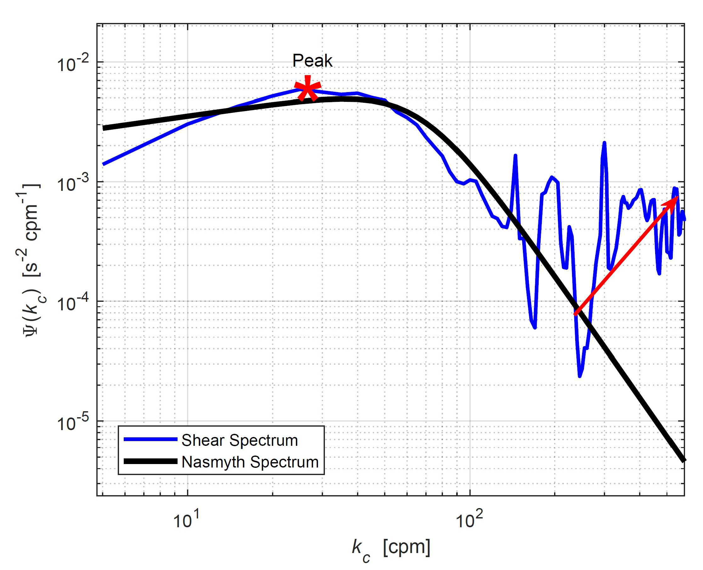
As mentioned in Section 2.1, $\chi$ and $ϵ$ values are measured by temperature spectrum and empirical Nasmyth spectrum. Comparing the shear spectrum with the Nasmyth spectrum for $<U>=0.167$ m/s at $x/M=37$ indicates an acceptable fitness between the graphs (Figure 2). The shear spectrum starts to rise at a wavenumber by a factor of 70 below its peak (Figure 2), which shows the spectrum contains more than 90 % of all shear variance as mentioned in Rockland scientific international note 28 [29].

This section uses four parts to represent the results of our experiment. Section 3.1 displays the power-law decay results and the modified grid-generated turbulence model. The changes in THF, $\chi$, and $ϵ$ within the surface boundary layer are presented in Section 3.2 and Section 3.3. Finally, the effects of non-breaking waves on the near-surface $ϵ$ are shown in Section 3.4.

3.1. Steady and Spatially Decaying Background Turbulence—Grid-Generated Turbulence

The VMP200 [27] measured $ϵ$, $\chi$, and temperature variance $<{\theta }^2>$ at a constant depth of $z=0.25$ m and selected distances along the tank centerline ($25<x/M<38$) for $<U>=0.183$ m/s. The data collected for $<U>=0.167$ were measured between $28<x/M<38$. We estimated a background heat flux of about 25 W/m${}^2$ from the equation of $Q=\mid \left(\rho C_p{K}_{\theta }\frac{\partial <T>}{\partial z}\right)/A_w\mid$ [56], where $A_w$ is the water surface area. It likely changes during the experiments (the measured background heat flux is the summation of heat transfer from all sides of the tank walls and the water surface through the whole length of the tank).

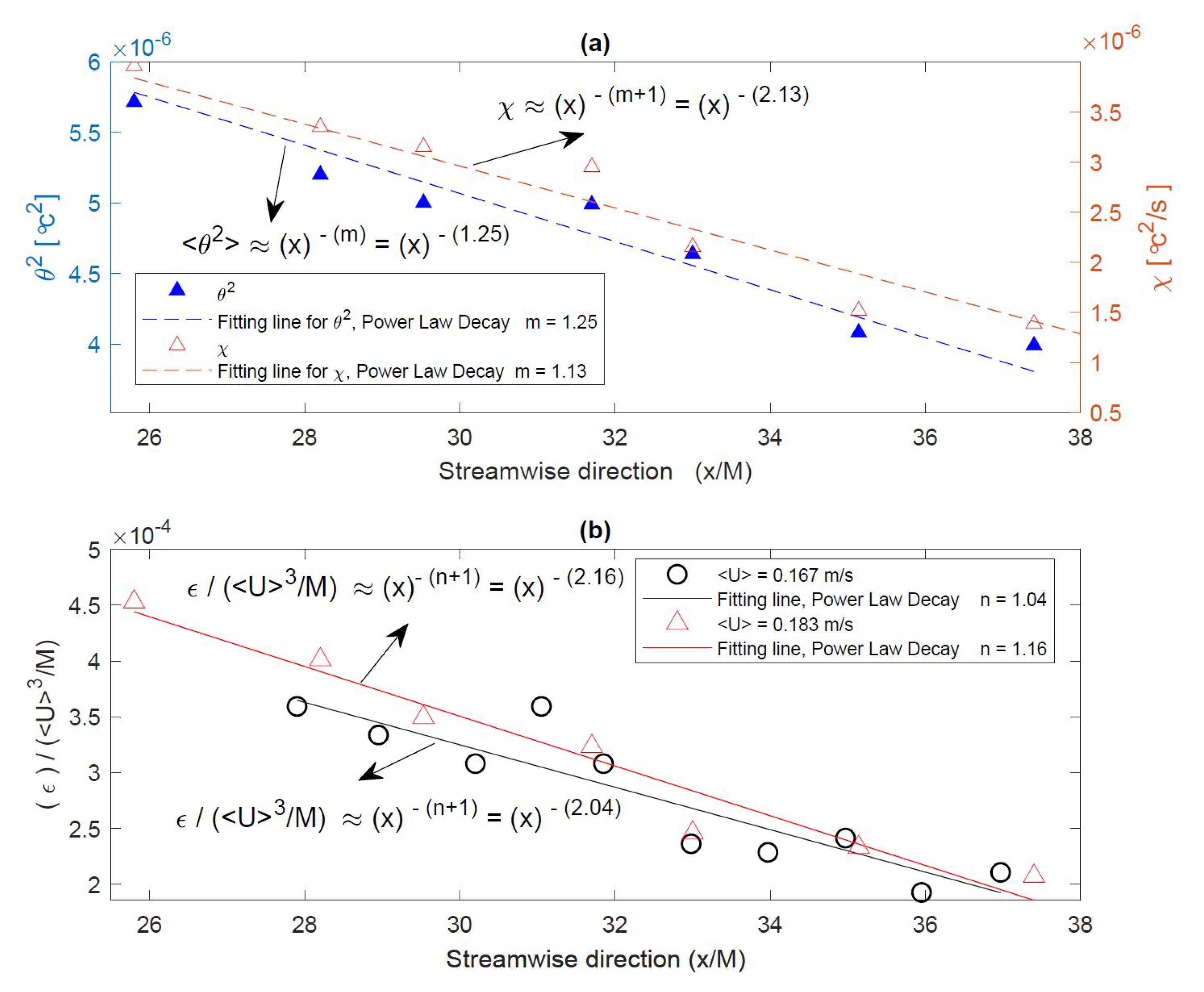
The linear fitting line is used to find the power-law exponent for $\chi$ and ${\theta }^2$ that they were $m=1.13$ and $m=1.25$, respectively (Figure 3). We found that the power-law exponent for the decay of $ϵ$ values was $n=1.04$ and 1.16 for the flow velocities of 0.167 m/s and 0.183 m/s, respectively (Figure 3). Based on the observed $ϵ$ and $\chi$ in our experiment (Figure 3) and following Zhou et al. [43] and Bogucki et al. [57], we found the following set of equations for $\chi$ and $ϵ$ as a function of mean flow velocity <U> and distance to turbulence-generating x:

$$\chi =0.2\times \frac{1}{<U>}\times P_0^2\times {(x/M)}^{-2.13}$$

(4)

and

$$ϵ=5\times <U{>}^3\times {(x/M)}^{-2.1}$$

(5)

The set of equations are defined due to observed m and n in our experiment. The values are considered to be as m + 1 = 1.13 + 1 = 2.13 for $\chi$ and the average of $n+1=(1.04+1.16)/2+1=2.1$ for $ϵ$. To have the $\chi$ in $[{}^{\circ }{\mathrm{C}}^2/\mathrm{s}]$ and $ϵ$ in $[{\mathrm{m}}^2/{\mathrm{S}}^3]$, the $<U>$ has to be expressed in $[\mathrm{m}/\mathrm{s}]$, the $P_0$ in [W], and the factors of 0.2 and 5 have units of $\left[\frac{{\mathrm{mc}}^2}{{\mathrm{j}}^2}\right]$, and $[1/\mathrm{m}]$, respectively.

3.2. Observations of Free Convective Flow and Associated Vertical Heat Flux

Data were collected at $x/M=37$, where the air–water temperature difference was approximately uniform during the experiment. The average net surface vertical heat flux of $Q\approx \mid 25\mid$ W/m${}^2$ in our experiment was not substantial in comparison to the mean range of net vertical heat flux in the ocean $Q<\mid 150\mid$ W/m${}^2$ [58], and also the heated-grid generated a horizontal heat flux of $16.6$ kW/m${}^2$, which is smaller than of the 5-year mean of the south China Sea front region ∼$4.6*{10}^2$ kW/m${}^2$ [59] (for a mixed boundary layer of $L_m=35$ m).

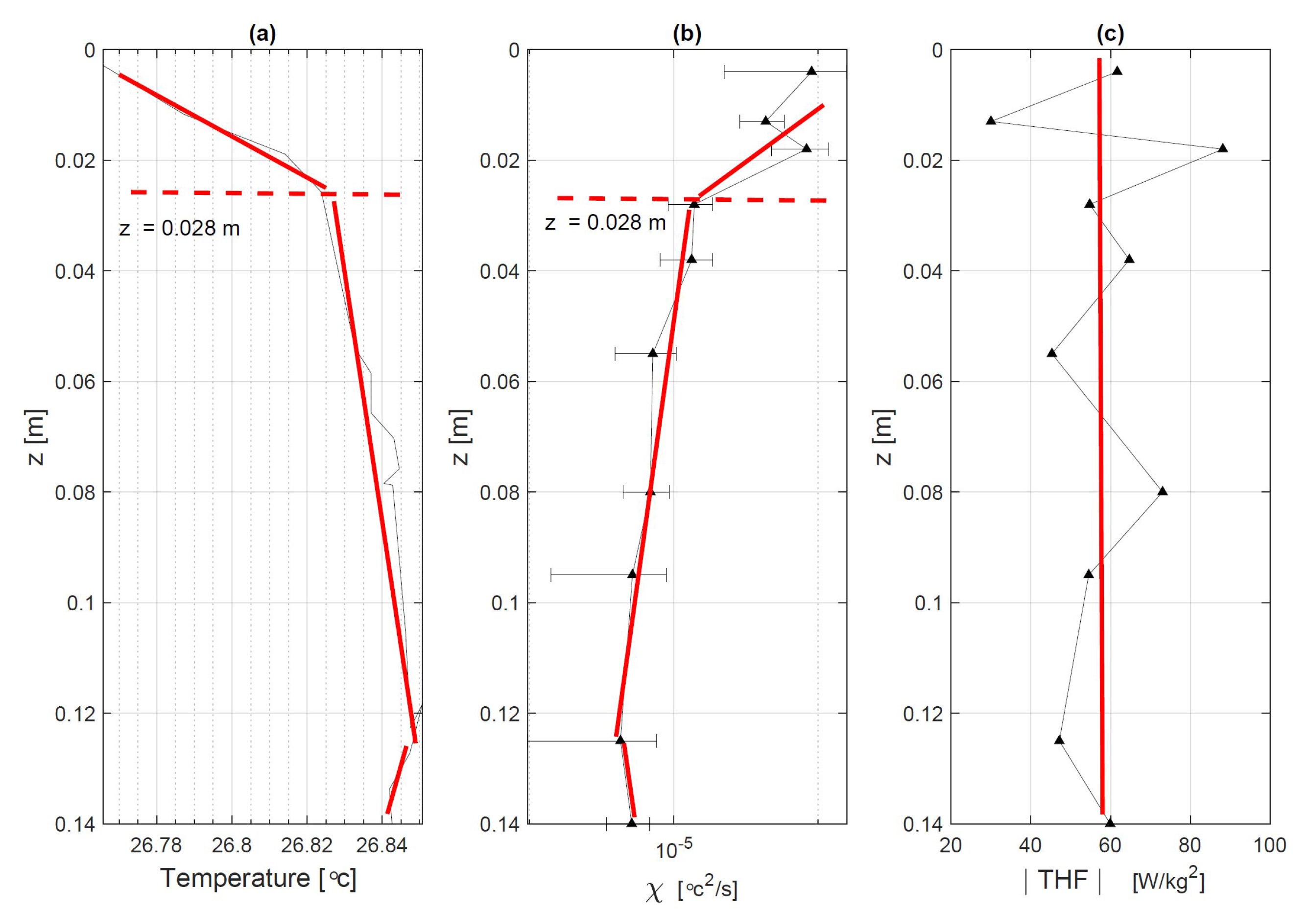
The surface heat flux increased the temperature gradient near the water surface, $z=0.028$ m up to the water surface (Figure 4a). Due to the water surface cooling, the positive temperature gradient results in the near-surface convection in our experiment. The temperature drives the density as, in our freshwater experiment, the salinity is close to zero in the entire water depth. The water density decreased about ≈$0.132$ kg m${}^3$ from the water surface to a depth of 0.14 m, causing an unstratified boundary layer.

An appropriate normalization method is not identified for $\chi$ values; therefore, $\chi$ values are depicted as non-normalized values in Figure 4b similar to the Bogucki et al. [12,13] and Peterson and Fer [36] works. Comparing $\chi$ (Figure 4a) and temperature (Figure 4b) reveals that the gradient of $\chi$ varies when the temperature gradient changes (it is shown with red lines). $\chi$ value increases by approaching the water surface (Figure 4b) as the temperature gradient increases, which shows that the large-scale vertical temperature gradient change, $d<T>/dz$, is consistent with the value of small-scale temperature fluctuation, $\chi$.

The average of the THF values (the red line shows it in Figure 4c) are approximately constant within the surface layer; however, the THF’s variance increases up to 50% at $0<z<0.028$ m, which is in the range of the wave-effected layer (see Figure 5c).

3.3. Vertical $ϵ$ Profile Observations

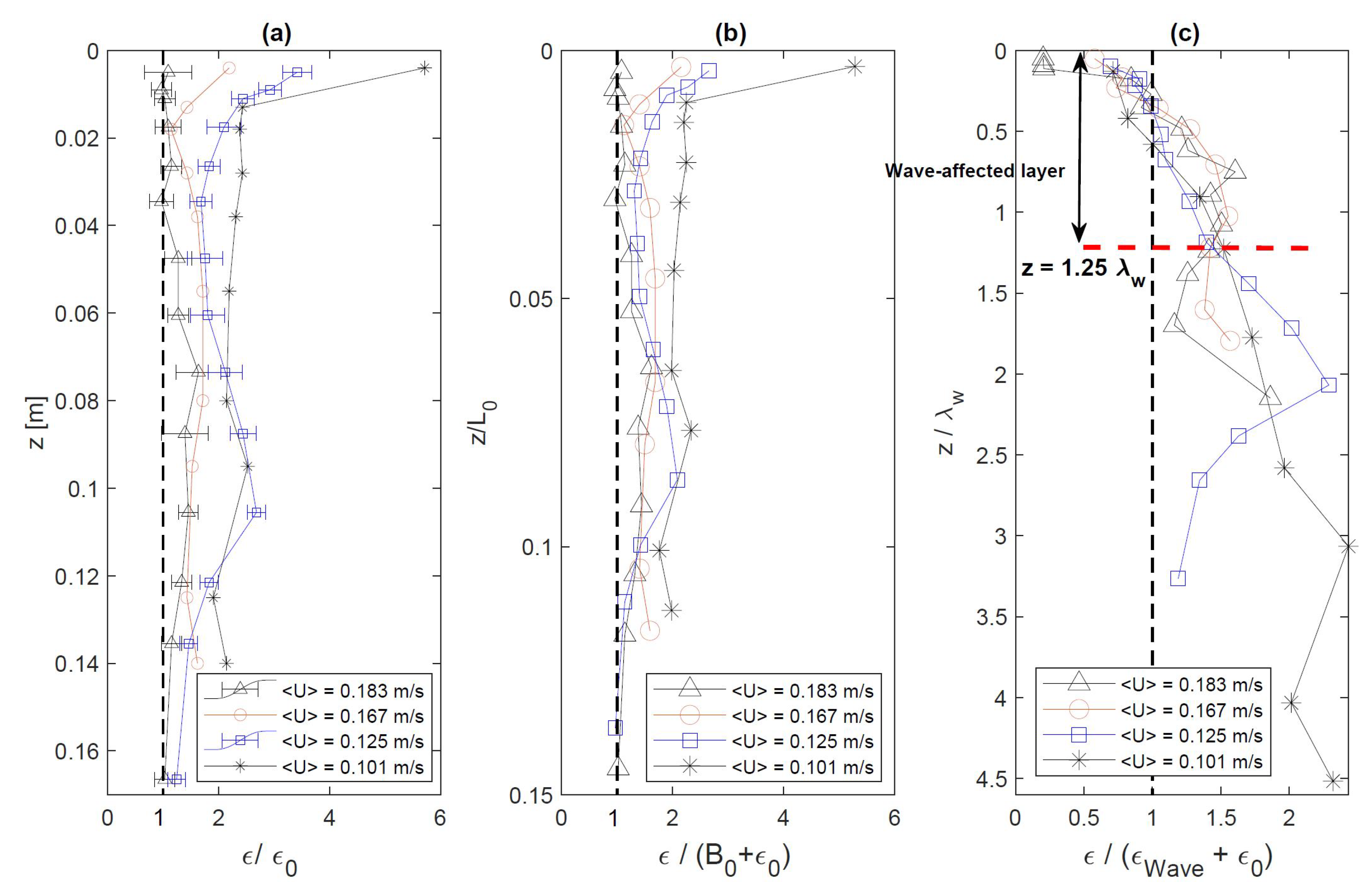
The data were collected at $x/M=37$ from a depth of $z=0.17$ m up to $z=0.005$ m to investigate the vertical $ϵ$ profile. Scaling of $ϵ$ aids in understanding and describing the boundary layer physics (Figure 5). $ϵ$ is normalized by the grid-generated turbulent kinetic energy dissipation rate called “background turbulence” ${ϵ}_0$ (Figure 5a). The surface buoyancy flux $B_0$ (Equation (5)) and the wave-generated turbulent kinetic energy dissipation rate ${ϵ}_{\mathrm{wave}}$ (Equation (3)) are also used to normalize $ϵ$ (Figure 5b,c).

${ϵ}_0$ was measured at the tank center ($z=0.25$ m). The background turbulence ranges between ${ϵ}_0\approx 0.5-3\times {10}^{-5}$ m${}^2$/s${}^3$ that are within the subset of ocean range, $ϵ\approx {10}^{-11}-{10}^{-3}$ m${}^2$/s${}^3$ [60,61,62]. The normalized $ϵ$ with background turbulence for different velocities converge together in deeper water; however, they diverge by approaching the water surface ($z>0.02$ m). In Figure 5b, $ϵ$ values are normalized with the summation of the surface buoyancy flux $B_0$ and background turbulence ${ϵ}_0$, i.e., $ϵ/(B_0+{ϵ}_0)$ (Figure 5b). The Obukhov length scale $L_0=k{u_{*}}^3/B_0$ [47] is used to normalize the water depth (Figure 5b), which characterizes the relative importance of the shear and buoyant convection in the boundary layer [47,63]. The change in $B_0$ for the mean flow velocity range of $0.066$ m/s to $0.183$ m/s was small ≈$2.8\%$ (Table 1) given that the air temperature, humidity, and water temperature did not change during the experiment. The similar rates for both scaling methods (Figure 5a,b) suggest that the background turbulence is larger than the turbulence generated with the surface convection, and the convergence of $ϵ/{ϵ}_0$ in depth indicates the dominance of the grid-generated turbulence.

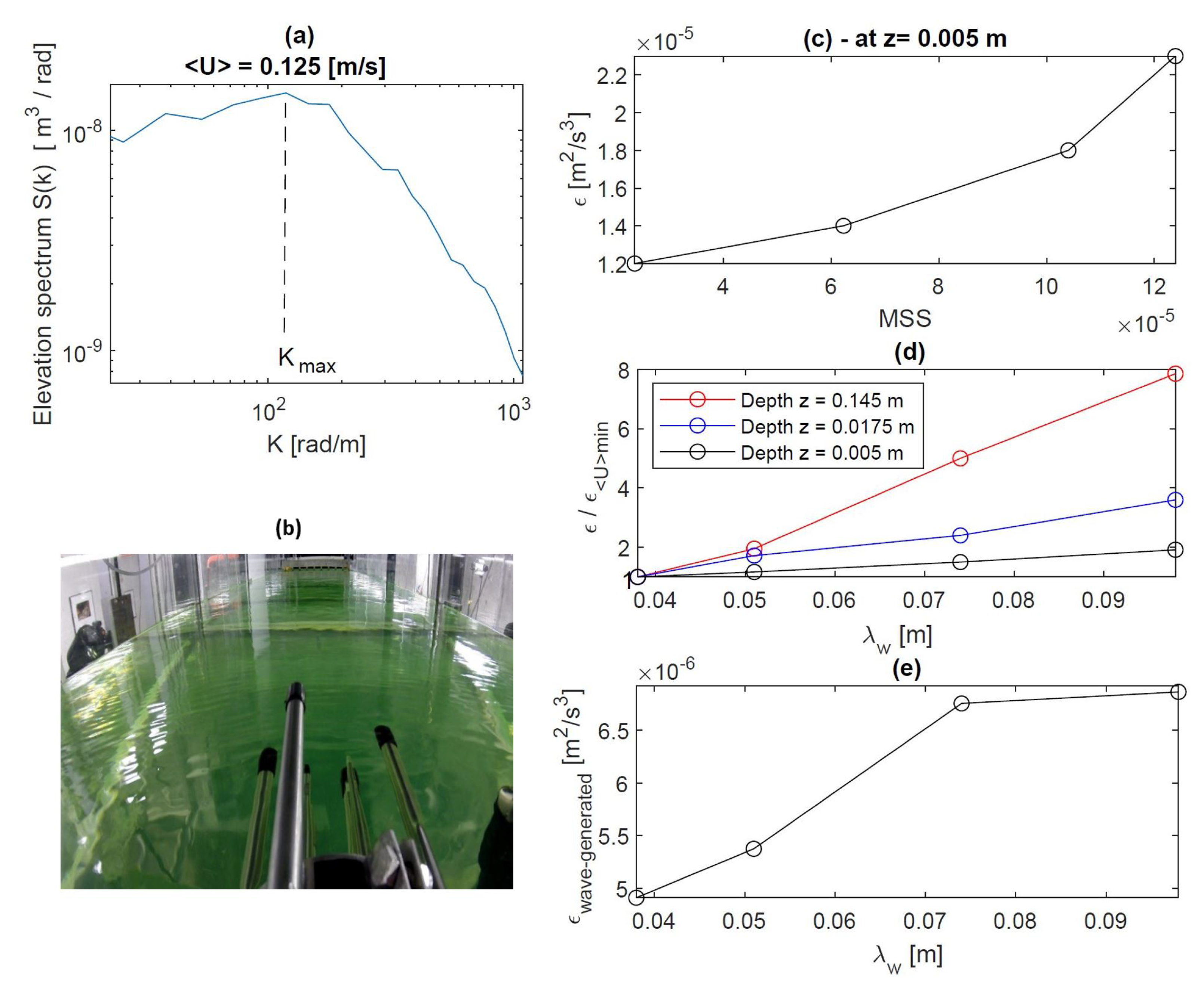
The non-breaking surface wave is another source of turbulence in addition to the surface convection. Given that the source of propagating waves is not clear, we must note that our wave-generated $ϵ$ measurements may not be truly representative of results that would be obtained in the field. The Doppler shifting correction [64,65] was performed on the surface elevation spectrum and graphed in Figure 6a for the mean flow velocity of $<U>=0.125$ m/s, which represented the presence of the surface waves. In addition to the surface elevation spectrum, the visual observations show that the uniform surface waves are created along the whole tank when the water moves along the tank with the grid (Figure 6b) and without the grid (the figure does not show) inside the tank. The wave number of elevation spectrum peak, $K_{max}$ (Figure 6a), is considered to calculate the wavelength ${\lambda }_{\mathrm{w}}$ of non-breaking waves. The wavelength ranges between 0.038 m $<{\lambda }_{\mathrm{w}}<0.098$ m (Table 1) categorized as the gravity or gravity-capillary regimes [22]. The integration of elevation spectrum S(K) gives the $<{\eta }^2>={\int }_0^{\infty }S\left(K\right)dK$ [42], hereupon the wave height $H=2<\eta >$.

The normalized $ϵ$ with the summation of the wave-generated turbulence ${ϵ}_{Wave}$, Equation (A9), and background turbulence, ${ϵ}_0$, i.e., $ϵ/({ϵ}_{Wave}+{ϵ}_0)$ are presented in Figure 5c. The normalized $ϵ$ values converge together from water surface to depth of $z=1.25{\lambda }_{\mathrm{w}}$ (Figure 5c), where the average of normalized $ϵ$ values is approximately one. This indicates that the wave-generated turbulence plays a dominant role on the near-surface $ϵ$ value in comparison to the surface convection and internal turbulence, and that is why the layer from the water surface to the depth of $z=1.25{\lambda }_{\mathrm{w}}$ is called the “wave-affected layer” in our paper.

3.4. Wave-Generated $ϵ$

The mean flow velocity increase resulted in the increment of the mean square slope (MSS) and wavelength ${\lambda }_{\mathrm{w}}$ (Table 1). $ϵ$ has a larger value while the MSS increases (Figure 6c), and they have the same order of magnitude, i.e., MSS $\sim ϵ$ below the water surface $z=0.005$ m. $ϵ$ for the different mean flow velocities were compared at three different depths (Figure 6d) to investigate the effects of the non-breaking surface wave and the grid-generated turbulence on $ϵ$ along the water column. Figure 6d indicates that at a depth of $z=0.145$ m, $ϵ$ change rate (red line) is higher than at $z=0.005$ m (black line) while the surface heat flux was constant.

The turbulent kinetic energy dissipation rate comparison between the mean flow velocity range of 0.066 m/s to 0.183 m/s at the different depths shows that $ϵ$ values increase ≈$780\%$, $370\%$, and $95\%$ at a depth of $z=0.145$ m, $z=0.0175$ m, and $z=0.005$ m, respectively (Figure 6d). By considering constant heat flux during the experiment, the $ϵ$ change rate should be the same when approaching the water surface if the grid was the only source of turbulence. The different change rates, like wave scaling results (Figure 5c), indicate that the non-breaking waves play a dominant role in $ϵ$ on the surface layer. The subtraction of the averaged-$ϵ$ within the wave-affected layer, ${ϵ}_{1.25{\lambda }_{\mathrm{w}}}$, from the background turbulent kinetic energy dissipation rate, ${ϵ}_0$, is considered the wave-generated turbulent kinetic energy dissipation rate, ${ϵ}_{\mathrm{wave}-\mathrm{generated}}={ϵ}_{1.25{\lambda }_{\mathrm{w}}}-{ϵ}_0$. The ${ϵ}_{\mathrm{wave}-\mathrm{generated}}$ for wavelength of 0.038 m <${\lambda }_{\mathrm{w}}$< 0.098 m ranged to $4.9\times {10}^{-6}-7\times {10}^{-6}$ m${}^2$/s${}^3$ (Figure 6e). Given that the breaking wave is often related to the enhanced turbulent kinetic energy dissipation rate within the surface layer, ${ϵ}_{\mathrm{wave}-\mathrm{generated}}$ values represent the significant role of non-breaking waves on the upper-ocean mixing intensity. It indicates that well-documented researches are necessary to shed light on the poor understanding of the non-breaking wave-generated turbulence. Furthermore, it depicts that the precise values of non-breaking wave-generated turbulent kinetic energy dissipation rate are required to quantify the air–sea interface processes.

4. Conclusions

Oceanic turbulence measurements are practically impossible when attempting to address processes within a few upper centimeters below the wave ocean surface. Our experiment aimed to investigate how the weak surface forcings and the horizontal heat and eddy fluxes affect the near-surface layer in a controlled laboratory setting like the front in the Gulf of Mexico where the Mississippi River with massive horizontal eddy fluxes reaches the ocean and generates the front. In our lab experiment, the internal $ϵ$ and horizontal heat flux generated by the grids were the subsets of the ocean $ϵ$ [60,61,62] and heat fluxes range [59].

While analyzing the vertical $ϵ$ variability, we have observed that there is a “wave-affected layer” from the water surface to a depth of $z\approx 1.25{\lambda }_{\mathrm{w}}$. Turbulence kinetic energy dissipation rate associated with non-breaking waves ${ϵ}_{\text{wave-generated}}$ ranged to $4.9\times {10}^{-6}$–$7\times {10}^{-6}$ m${}^2$/s${}^3$ for the wavelength range of 0.038 m <${\lambda }_{\mathrm{w}}$< 0.098 m categorized as the gravity and gravity-capillary regimes [21,22,23]. The increase in the MSS resulted in the larger $ϵ$, and they have the same order of magnitude MSS $\sim ϵ$. Given that the non-breaking waves typically cover a larger fraction of the ocean surface, 90–100% [17], than breaking waves, the $ϵ$ results indicate their significant contribution to the ocean energy budget. Therefore, the non-breaking wave’s turbulence kinetic energy dissipation rate budget has to be considered to properly quantify the air–sea interface processes such as cool skin thickness [66], which is a fundamental parameter required for quantifying the physical process taking place at the air=-sea interface like the gas transfer [4] and heat transfer [67].

We also found that $\chi$ changes, which is the small-scale temperature fluctuation, are consistent with the large-scale temperature gradient, $d<T>/dz$, changes. The value of the THF is approximately constant within the surface layer. It represents that the measured THF near the water surface can be considered a surface water THF in the ocean, challenging to measure directly.

In addition, we observed that the power-law exponent of the tank is $m=1.13$ and $m=1.25$ for the decay of $\chi$ and temperature variance $<{\theta }^2>$, respectively, and the decay of $ϵ$ equals $n=1.04$ and $n=1.16$ for the velocities $0.167$ m/s and $0.183$ m/s.

The future work would be to connect the laboratory observation to the field observation. We will explore whether the THF value is constant within the upper ocean boundary layer as observed in this research. We would also like to study the importance of $ϵ$ below the non-breaking gravity wave and investigate if the observed affected layer in this paper is common properties below the non-breaking and breaking waves in the ocean.

References

- Terashima, H. The Importance of Education and Capacity-building Programs for Ocean Govemance. Ocean Yearb. Online 2004, 18, 600–611. [Google Scholar] [CrossRef]
- Dourado, M.; Oliveira, A.P.D. Observational description of the atmospheric and oceanic boundary layers over the Atlantic Ocean. Rev. Bras. Oceanogr. 2001, 49, 49–59. [Google Scholar] [CrossRef]
- Pinker, R.T.; Bentamy, A.; Katsaros, K.; Ma, Y.; Li, C. Estimates of net heat fluxes over the Atlantic Ocean. J. Geophys. Res. Ocean. 2014, 119, 410–427. [Google Scholar] [CrossRef] [Green Version]
- Fredriksson, S.T.; Arneborg, L.; Nilsson, H.; Zhang, Q.; Handler, R.A. An evaluation of gas transfer velocity parameterizations during natural convection using DNS. J. Geophys. Res. Ocean. 2016, 121, 1400–1423. [Google Scholar] [CrossRef]
- Loh, A.; Shankar, R.; Ha, S.Y.; An, J.G.; Yim, U.H. Stability of mechanically and chemically dispersed oil: Effect of particle types on oil dispersion. Sci. Total Environ. 2020, 716, 135343. [Google Scholar] [CrossRef]
- Ramírez, J.; Moghimi, S.; Restrepo, J.M.; Venkataramani, S. Modelling the mass exchange dynamics of oceanic surface and subsurface oil. Ocean Model. 2018, 129, 1–12. [Google Scholar] [CrossRef] [Green Version]
- Pope, S.B. Turbulent Flows. 2001. Available online: https://0-iopscience-iop-org.brum.beds.ac.uk/article/10.1088/0957-0233/12/11/705/meta (accessed on 18 February 2021).
- Metoyer, S.; Barzegar, M.; Bogucki, D.; Haus, B.K.; Shao, M. Measurement of small-scale surface velocity and turbulent kinetic energy dissipation rates using infrared imaging. J. Atmos. Ocean. Technol. 2020, 38. [Google Scholar] [CrossRef]
- Wain, D.J.; Lilly, J.M.; Callaghan, A.H.; Yashayaev, I.; Ward, B. A breaking internal wave in the surface ocean boundary layer. J. Geophys. Res. Ocean. 2015, 120, 4151–4161. [Google Scholar] [CrossRef] [Green Version]
- Wang, D.W.; Wijesekera, H.W. Observations of breaking waves and energy dissipation in modulated wave groups. J. Phys. Oceanogr. 2018, 48, 2937–2948. [Google Scholar] [CrossRef]
- Bogucki, D.; Haus, B.K.; Shao, M. The dissipation of energy beneath non-breaking waves. In Proceedings of the Ocean Sciences Meeting 2020, AGU, San Diego, CA, USA, 19 February 2020. [Google Scholar]
- Bogucki, D.J.; Huguenard, K.; Haus, B.K.; Özgökmen, T.; Reniers, A.; Laxague, N. Scaling laws for the upper ocean temperature dissipation rate. Geophys. Res. Lett. 2015, 42, 839–846. [Google Scholar] [CrossRef] [Green Version]
- Bogucki, D.; Haus, B.K.; Shao, M. The Response of the Boundary Layer to Weak Forcing. In Proceedings of the Ocean Sciences Meeting 2020, AGU, San Diego, CA, USA, 19 February 2020. [Google Scholar]
- Berhanu, M.; Falcon, E.; Deike, L. Turbulence of capillary waves forced by steep gravity waves. J. Fluid Mech. 2018, 850, 803–843. [Google Scholar] [CrossRef] [Green Version]
- Wüest, A.; Piepke, G.; Van Senden, D.C. Turbulent kinetic energy balance as a tool for estimating vertical diffusivity in wind-forced stratified waters. Limnol. Oceanogr. 2000, 45, 1388–1400. [Google Scholar] [CrossRef]
- Terray, E.; Donelan, M.; Agrawal, Y.; Drennan, W.M.; Kahma, K.; Williams, A.J.; Hwang, P.; Kitaigorodskii, S. Estimates of kinetic energy dissipation under breaking waves. J. Phys. Oceanogr. 1996, 26, 792–807. [Google Scholar] [CrossRef] [Green Version]
- Anguelova, M.D.; Webster, F. Whitecap coverage from satellite measurements: A first step toward modeling the variability of oceanic whitecaps. J. Geophys. Res. Ocean. 2006, 111. [Google Scholar] [CrossRef] [Green Version]
- Babanin, A.V.; Haus, B.K. On the existence of water turbulence induced by nonbreaking surface waves. J. Phys. Oceanogr. 2009, 39, 2675–2679. [Google Scholar] [CrossRef]
- Bogucki, D.J.; Haus, B.K.; Barzegar, M.; Shao, M.; Domaradzki, J.A. On the Nature of the Turbulent Energy Dissipation Beneath Nonbreaking Waves. Geophys. Res. Lett. 2020, 47, e2020GL090138. [Google Scholar] [CrossRef]
- Barkan, R.; McWilliams, J.C.; Shchepetkin, A.F.; Molemaker, M.J.; Renault, L.; Bracco, A.; Choi, J. Submesoscale dynamics in the northern Gulf of Mexico. Part I: Regional and seasonal characterization and the role of river outflow. J. Phys. Oceanogr. 2017, 47, 2325–2346. [Google Scholar] [CrossRef]
- Munk, W.H. Origin and Generation of Waves; Technical Report; Scripps Institution of Oceanography: La Jolla, CA, USA, 1951. [Google Scholar]
- Laxague, N.J.M. Development and Application of Gravity-Capillary Wave Fourier Analysis for the Study of Air-Sea Interaction Physics; University of Miami: Coral Gables, FL, USA, 2016. [Google Scholar]
- Chen, P.; Wang, X.; Liu, L.; Chong, J. A coupling modulation model of capillary waves from gravity waves: Theoretical analysis and experimental validation. J. Geophys. Res. Ocean. 2016, 121, 4228–4244. [Google Scholar] [CrossRef]
- Murzyn, F.; Bélorgey, M. Experimental investigation of the grid-generated turbulence features in a free surface flow. Exp. Therm. Fluid Sci. 2005, 29, 925–935. [Google Scholar] [CrossRef]
- Grzelak, J.; Wierciński, Z. The decay power law in turbulence generated by grids. Trans. Inst. Fluid-Flow Mach. 2015, 130, 93–107. [Google Scholar]
- Tennekes, H.; Lumley, J.L.; Lumley, J. A First Course in Turbulence; MIT Press: Cambridge, MA, USA, 1972. [Google Scholar]
- Lueck, R.G.; Wolk, F.; Yamazaki, H. Oceanic velocity microstructure measurements in the 20th century. J. Oceanogr. 2002, 58, 153–174. [Google Scholar] [CrossRef]
- Macoun, P.; Lueck, R. Modeling the spatial response of the airfoil shear probe using different sized probes. J. Atmos. Ocean. Technol. 2004, 21, 284–297. [Google Scholar] [CrossRef]
- Lueck, R. Calculating the Rate of Dissipation of Turbulent Kinetic Energy; RSI Technical Note 028; Rockland Scientific International Inc.: Victoria, BC, Canada, 2013; Volume 18. [Google Scholar]
- Lueck, R. Converting Shear Probe, Thermistors and Microconductivity Signals into Physical Units; Rockland Scientific International Inc.: Victoria, BC, Canada, 2010; Volume 1. [Google Scholar]
- Siddon, T.E.; Ribner, H.S. An aerofoil probe for measuring the transverse component of turbulence. AIAA J. 1965, 3, 747–749. [Google Scholar] [CrossRef]
- Osborn, T.; Crawford, W. An airfoil probe for measuring turbulent velocity fluctuations in water. In Air-Sea Interaction; Springer: Berlin/Heidelberg, Germany, 1980; pp. 369–386. [Google Scholar]
- Bluteau, C.E.; Lueck, R.G.; Ivey, G.N.; Jones, N.L.; Book, J.W.; Rice, A.E. Determining mixing rates from concurrent temperature and velocity measurements. J. Atmos. Ocean. Technol. 2017, 34, 2283–2293. [Google Scholar] [CrossRef]
- Goodman, L.; Levine, E.R.; Lueck, R.G. On measuring the terms of the turbulent kinetic energy budget from an AUV. J. Atmos. Ocean. Technol. 2006, 23, 977–990. [Google Scholar] [CrossRef] [Green Version]
- Kolmogorov, A.N. The local structure of turbulence in incompressible viscous fluid for very large Reynolds numbers. Proc. R. Soc. Lond. Ser. A Math. Phys. Sci. 1991, 434, 9–13. [Google Scholar]
- Peterson, A.K.; Fer, I. Dissipation measurements using temperature microstructure from an underwater glider. Methods Oceanogr. 2014, 10, 44–69. [Google Scholar] [CrossRef] [Green Version]
- Oakey, N. Determination of the rate of dissipation of turbulent energy from simultaneous temperature and velocity shear microstructure measurements. J. Phys. Oceanogr. 1982, 12, 256–271. [Google Scholar] [CrossRef] [Green Version]
- Bogucki, D.; Luo, H.; Domaradzki, J. Experimental evidence of the Kraichnan scalar spectrum at high reynolds numbers. J. Phys. Oceanogr. 2012, 42, 1717–1728. [Google Scholar] [CrossRef]
- Lueck, R.G.; Hertzman, O.; Osborn, T.R. The spectral response of thermistors. Deep Sea Res. 1977, 24, 951–970. [Google Scholar] [CrossRef]
- Nash, J.D.; Caldwell, D.R.; Zelman, M.J.; Moum, J.N. A thermocouple probe for high-speed temperature measurement in the ocean. J. Atmos. Ocean. Technol. 1999, 16, 1474–1482. [Google Scholar] [CrossRef] [Green Version]
- Donelan, M.A.; Plant, W.J. A threshold for wind-wave growth. J. Geophys. Res. Ocean. 2009, 114. [Google Scholar] [CrossRef] [Green Version]
- Elfouhaily, T.; Chapron, B.; Katsaros, K.; Vandemark, D. A unified directional spectrum for long and short wind-driven waves. J. Geophys. Res. Ocean. 1997, 102, 15781–15796. [Google Scholar] [CrossRef]
- Zhou, T.; Antonia, R.; Danaila, L.; Anselmet, F. Transport equations for the mean energy and temperature dissipation rates in grid turbulence. Exp. Fluids 2000, 28, 143–151. [Google Scholar] [CrossRef]
- Antonia, R.; Zhou, T.; Zhu, Y. Three-component vorticity measurements in a turbulent grid flow. J. Fluid Mech. 1998, 374, 29–57. [Google Scholar] [CrossRef]
- Hearst, R.J.; Lavoie, P. Decay of turbulence generated by a square-fractal-element grid. J. Fluid Mech. 2014, 741, 567–584. [Google Scholar] [CrossRef] [Green Version]
- Warhaft, Z.; Lumley, J. An experimental study of the decay of temperature fluctuations in grid-generated turbulence. J. Fluid Mech. 1978, 88, 659–684. [Google Scholar] [CrossRef]
- Soloviev, A.; Klinger, B.; Steele, J.; Thorpe, S. Open ocean convection. Encycl. Ocean Sci. 2001, 4, 2015–2022. [Google Scholar]
- Moum, J.N. Energy-containing scales of turbulence in the ocean thermocline. J. Geophys. Res. Ocean. 1996, 101, 14095–14109. [Google Scholar] [CrossRef]
- Osborn, T.R.; Cox, C.S. Oceanic fine structure. Geophys. Astrophys. Fluid Dyn. 1972, 3, 321–345. [Google Scholar] [CrossRef]
- Ruddick, B.; Walsh, D.; Oakey, N. Variations in apparent mixing efficiency in the North Atlantic Central Water. J. Phys. Oceanogr. 1997, 27, 2589–2605. [Google Scholar] [CrossRef]
- Esters, L.; Breivik, Ø.; Landwehr, S.; ten Doeschate, A.; Sutherland, G.; Christensen, K.H.; Bidlot, J.R.; Ward, B. Turbulence scaling comparisons in the ocean surface boundary layer. J. Geophys. Res. Ocean. 2018, 123, 2172–2191. [Google Scholar] [CrossRef]
- Kitaigorodskii, S.; Donelan, M.; Lumley, J.; Terray, E. Wave-turbulence interactions in the upper ocean. part ii. statistical characteristics of wave and turbulent components of the random velocity field in the marine surface layer. J. Phys. Oceanogr. 1983, 13, 1988–1999. [Google Scholar] [CrossRef] [Green Version]
- Gargett, A.E. Ocean turbulence. Annu. Rev. Fluid Mech. 1989, 21, 419–451. [Google Scholar] [CrossRef]
- Sutherland, G.; Ward, B.; Christensen, K. Wave-turbulence scaling in the ocean mixed layer. Ocean Sci. 2013, 9, 597–608. [Google Scholar] [CrossRef] [Green Version]
- Zahariev, K.; Garrett, C. An apparent surface buoyancy flux associated with the nonlinearity of the equation of state. J. Phys. Oceanogr. 1997, 27, 362–368. [Google Scholar] [CrossRef]
- Wells, A.J.; Cenedese, C.; Farrar, J.T.; Zappa, C.J. Variations in ocean surface temperature due to near-surface flow: Straining the cool skin layer. J. Phys. Oceanogr. 2009, 39, 2685–2710. [Google Scholar] [CrossRef] [Green Version]
- Bogucki, D.J.; Domaradzki, J.A.; von Allmen, P. Polarimetric lidar measurements of aquatic turbulence-laboratory experiment. Opt. Express 2018, 26, 6806–6816. [Google Scholar] [CrossRef] [PubMed]
- Carton, J.A.; Chepurin, G.A.; Chen, L.; Grodsky, S.A. Improved global net surface heat flux. J. Geophys. Res. Ocean. 2018, 123, 3144–3163. [Google Scholar] [CrossRef]
- Pan, J.; Sun, Y. Estimation of Horizontal Eddy Heat Flux in Upper Mixed-Layer in the South China Sea by Using Satellite Data. Sci. Rep. 2018, 8, 1–11. [Google Scholar] [CrossRef] [Green Version]
- McMillan, J.M.; Hay, A.E.; Lueck, R.G.; Wolk, F. Rates of dissipation of turbulent kinetic energy in a high Reynolds number tidal channel. J. Atmos. Ocean. Technol. 2016, 33, 817–837. [Google Scholar] [CrossRef]
- Lozovatsky, I.; Fernando, H.; Planella-Morato, J.; Liu, Z.; Lee, J.H.; Jinadasa, S. Probability distribution of turbulent kinetic energy dissipation rate in ocean: Observations and approximations. J. Geophys. Res. Ocean. 2017, 122, 8293–8308. [Google Scholar] [CrossRef]
- Evans, D.G.; Lucas, N.S.; Hemsley, V.; Frajka-Williams, E.; Naveira Garabato, A.C.; Martin, A.; Painter, S.C.; Inall, M.E.; Palmer, M.R. Annual cycle of turbulent dissipation estimated from Seagliders. Geophys. Res. Lett. 2018, 45, 10–560. [Google Scholar] [CrossRef] [Green Version]
- Markowski, P.M.; Lis, N.T.; Turner, D.D.; Lee, T.R.; Buban, M.S. Observations of near-surface vertical wind profiles and vertical momentum fluxes from VORTEX-SE 2017: Comparisons to Monin–Obukhov similarity theory. Mon. Weather Rev. 2019, 147, 3811–3824. [Google Scholar] [CrossRef]
- Drennan, W.M.; Donelan, M.; Madsen, N.; Katsaros, K.; Terray, E.A.; Flagg, C. Directional wave spectra from a Swath ship at sea. J. Atmos. Ocean. Technol. 1994, 11, 1109–1116. [Google Scholar] [CrossRef] [Green Version]
- Collins, C., III; Blomquist, B.; Persson, O.; Lund, B.; Rogers, W.; Thomson, J.; Wang, D.; Smith, M.; Doble, M.; Wadhams, P.; et al. Doppler correction of wave frequency spectra measured by underway vessels. J. Atmos. Ocean. Technol. 2017, 34, 429–436. [Google Scholar] [CrossRef] [Green Version]
- Alappattu, D.P.; Wang, Q.; Yamaguchi, R.; Lind, R.J.; Reynolds, M.; Christman, A.J. Warm layer and cool skin corrections for bulk water temperature measurements for air-sea interaction studies. J. Geophys. Res. Ocean. 2017, 122, 6470–6481. [Google Scholar] [CrossRef]
- Liu, Y.; Yu, L.; Chen, G. Characterization of Sea Surface Temperature and Air-Sea Heat Flux Anomalies Associated with Mesoscale Eddies in the South China Sea. J. Geophys. Res. Ocean. 2020, 125, e2019JC015470. [Google Scholar] [CrossRef]
- Batchelor, G.K.; Townsend, A.A. Decay of isotropic turbulence in the initial period. Proc. R. Soc. Lond. Ser. A Math. Phys. Sci. 1948, 193, 539–558. [Google Scholar]
- Tresso, R.; Munoz, D.R. Homogeneous, isotropic flow in grid generated turbulence. J. Fluids Eng. 2000, 122, 51–56. [Google Scholar] [CrossRef]
- Gemmrich, J. Strong turbulence in the wave crest region. J. Phys. Oceanogr. 2010, 40, 583–595. [Google Scholar] [CrossRef]
Figure 1.
(a) A schematic of the Air–Sea Interaction Saltwater Tank (ASIST) tank at the University of Miami. Heated grid and grid-generated turbulence were installed at the tank entrance. The vertical microstructure profiler (VMP), laser slope, and current meter locations from turbulence generating grid are shown by . The insets indicate a side view of the instrument’s vertical position at the tank with a freshwater level of m and the turbulence generating grid’s mesh shape. (b) A schematic of internal and surface sources of turbulence. The blue arrows show the direction of the mean flow velocity. The swirl lines represent the background or internal turbulence generated by the grid.
Figure 2.
Comparison of the Shear spectrum with Nasmyth spectrum for <U> = 0.167 m/s at and depth of m. is wave number in the unit of cpm that it equals to . The spectrum peak is shown with a red star, and the red arrow shows the rising part of the spectrum.
Figure 3.
(a) Temperature variance () and values along the streamwise direction are shown. The dashed blue and brown lines are fitting lines of the and profiles, respectively. The mean flow velocity was m s. (b) The normalized value of along the streamwise direction is shown. The black and red lines are fitting lines of the data for 0.167 m/s and 0.183 m/s, respectively. The data were collected at m. The heated-grid power was kW for both graphs (a,b).
Figure 4.
(a) The vertical profiles of temperature, (b) with associated error bars, and (c) turbulent heat flux . The data for all three graphs were collected at a downstream distance of . The mean flow velocity is m/s, and the heater power was kW. The dashed red lines show the depth that the temperature and gradient changes. The graph fitting lines are presented with red lines. Note, the near-surface turbulent heat flux (THF) is approximately constant, as denoted by the red line segment (c).
Figure 5.
vertical profile is shown for the mean flow velocity range of 0.101 m/s< < 0.183 m/s. The data were measured at a depth of m to m at the downstream distance of . (a) is normalized by the background, or internal, turbulence kinetic energy dissipation rate generated by the grid, . The associated error bars are depicted for = 0.125 m/s and 0.183 m/s. (b) is normalized by the summation of surface buoyancy flux, , and . (c) The is normalized by the summation of wave-generated turbulent kinetic energy dissipation rate, , and . The wave-affected layer is presented with the dashed red line.
Figure 6.
(a) The surface elevation spectrum for the mean flow velocity of m/s is shown. The wavenumber related to the spectrum peak is shown by . (b) The non-breaking surface wave generated for m/s while the grid is located inside the tank. (c) The change for different mean square slope (MSS) is depicted at a depth of m. (d) The normalized value of different flow velocities is shown at three depths. The values are normalized with the of the lowest mean flow velocity of each depth, . (e) The subtraction of the averaged- within the wave-affected layer, , from the background turbulent kinetic energy dissipation rate, , is considered as the wave-generated turbulent kinetic energy dissipation rate, . The data were collected at the downstream distance of .