Wave Propagation Studies in Numerical Wave Tanks with Weakly Compressible Smoothed Particle Hydrodynamics

Abstract

Generation and propagation of waves in a numerical wave tank constructed using Weakly Compressible Smoothed Particle Hydrodynamics (WCSPH) are considered here. Numerical wave tank simulations have been carried out with implementations of different Wendland kernels in conjunction with different numerical dissipation schemes. The simulations were accelerated by using General Process Graphics Processing Unit (GPGPU) computing to utilize the massively parallel nature of the simulations and thus improve process efficiency. Numerical experiments with short domains have been carried out to validate the dissipation schemes used. The wave tank experiments consist of piston-type wavemakers and appropriate passive absorption arrangements to facilitate comparisons with theoretical predictions. The comparative performance of the different numerical wave tank experiments was carried out on the basis of the hydrostatic pressure and wave surface elevations. The effect of numerical dissipation with the different kernel functions was also studied on the basis of energy analysis. Finally, the observations and results were used to arrive at the best possible numerical set up for simulation of waves at medium and long distances of propagation, which can play a significant role in the study of extreme waves and energy localizations observed in oceans through such numerical wave tank simulations.

1. Introduction

Smoothed Particle Hydrodynamics (SPH) [1,2] is a meshless, Lagrangian, particle-based numerical method. It has been widely used over the past few decades for astrophysical simulations and understanding of hydrodynamic flows in coastal and marine engineering. Different numerical models can be used for these numerical simulations, mainly depending upon the complexity of the underlying equations, the size of the simulation domain and the resolution, among other factors. These influence the computational cost and thereby the choice of the model. Numerical methods based on a Eulerian approach like IHFOAM (a three-dimensional numerical solver for simulation of coastal engineering scenarios) [3] and COBRAS (Cornell Breaking Waves and Structure) [4] are used for a wide range of coastal engineering applications with a high degree of accuracy, but they also pose a number of problems in many situations. The computational mesh is required to overlap with all regions where the material is to move, even if the material occupies only a small part of the whole domain at a certain point in time. This results in a reduced resolution of the numerical solution and increased computational costs. Furthermore, models based on the Eulerian method require special treatment to track the positions of free surface particles and moving interfaces.

On the other hand, Lagrangian methods, which can be used to intrinsically track the motion of the free surface particles [5], are an excellent option for the simulation of hydrodynamic flows in wave tanks. Being meshless in nature, Lagrangian methods also make it easier to simulate flows involving complex geometries and those exhibiting violent phenomena like wave breaking, impact on structures or other surface-surface interactions, in contrast to the grid-based methods. Despite the clear advantages that Lagrangian methods like SPH can offer in simulating free surface hydrodynamic phenomena, they have a serious drawback in that they require a large amount of computational resources, especially those employing Navier-Stokes equations for more realistic simulations. SPH, however, belongs to a class of particle methods that can be accelerated using general-purpose computing on a graphics processor unit (GPGPU). This is done with the help of sorting and binning algorithms, which help reduce the computational complexity from O (${\mathrm{N}}^2$) to O (N logN). In an earlier work from this group, Chabalko and Balachandran [6] detailed the acceleration process of a similar particle method. The use of such computing techniques and increase in computational powers over the years has greatly contributed to an increase in applications of SPH in hydrodynamic simulations.

In SPH, the computational domain is discretized into a number of particles, with each particle representing a small volume of the fluid with the respective mass, density, velocity and other mechanical quantities associated with that volume. An interpolation scheme is then used to evaluate the mechanical quantities of all the particles over time using a weighted average of the properties of the adjacent particles within a certain domain as described by a kernel function. Liu [7] provided a general approach to devise analytical smoothing functions, pointing out that smoother second derivatives of kernel functions lead to better numerical stability. Adjustable support domains lend better flexibility and accuracy for kernel functions, as pointed out by Yang et al. [8]. At present, the cubic spline function [9] and the Wendland C2 function [10] are the most popular smoothing kernel functions. Using numerical convergence and linear stability tests, Dehnen and Aly [11] found out that Wendland kernels are computationally more convenient and exhibit better numerical convergence at large neighbor numbers ($N_H$) compared to the traditional B-spline kernels and present an excellent choice as smoothing functions in SPH. The Wendland C2 function that is commonly used as a smoothing kernel in SPH literature over the years is a 5th-degree class 2 Wendland kernel. Other Wendland functions mentioned by Dehnen and Aly include the 8th-degree class 4 kernel and the 11th-degree class 6 kernel functions, commonly known as the Wendland C4 and the Wendland C6 smoothing functions. Despite the use of the higher-order Wendland kernels for astrophysical simulations and computing the consistency and truncation errors in integrals [12,13], they have not been used in coastal engineering applications to the best of knowledge of the authors.

Numerical dissipation schemes also have an important role in WCSPH numerical methods helping to dissipate the spurious density and pressure oscillations generated due to the weakly compressible nature of the approach. Numerous approaches have been suggested for this, with the most notable ones being the artificial viscosity term implemented by Monaghan [14], the density reinitialization procedure [15] based on the Shephard filter, and the density dissipation terms by Ferrari et al. [16], Molteni and Colagrossi [17], and relatively recently by Antuono et al. [18]. Implementations of different numerical schemes have been found to more suitable for different types of WCSPH simulations. Morris et al. [19] developed a viscosity scheme for low Reynold number flows, which worked better than the traditional artificial viscosity scheme. The $\delta$-SPH scheme developed by Molteni and Colagrossi is more suited for damping out pressure or density fluctuations compared to the artificial viscosity scheme or the density reinitialization procedure. An improved $\delta$-SPH scheme where numerical dissipation is modified according to requirements in a complex flow has been developed recently [20].

Long-duration numerical wave tank experiments provide an excellent alternative to physical models in coastal engineering applications, especially when resources and scale effects are considered. Fundamental to such numerical wave tank experiments is the generation of waves that are able to propagate over the duration of the simulation without dissipating almost immediately, which is a possibility in SPH if the parameters used are inappropriate. Many studies have been carried out over the years to investigate the generation of waves in numerical modeling. Biesel and Suqet [21] gave a solution for the first-order wavemaker theory for piston-type wavemakers, which was subsequently improved by authors like Ursell et al. [22] and Schaffer [23]. However, when first-order wavemaker theory is used, the experimental flumes give rise to spurious secondary waves [24]. Madsen [25] suggested an approximate solution to this by providing an expression to eliminate the spurious secondary waves, which is accurate and computationally simple for generating waves of second order, although within a range. Later, Schaffer [23] gave a complete solution to the second-order wavemaker problem. After utilizing Madsen’s implementation, Altomare et al. [26] carried out long-crested wave generation for SPH-based models over medium distances to validate against theoretical and experimental observations. More recently, Trimulyono et al. [27] also made use of the DualSPHysics [28] model to simulate waves over long distances and validate the findings against experimental observations. Numerical wave tank experiments, if validated properly with theoretical and experimental findings, can also open up avenues for further studies on extreme waves [29] in oceans, which is increasingly gaining interest among engineers and scientists all over the world. A number of such SPH studies using numerical wave tanks have been undertaken in the past to investigate wave focusing and breaking. Manolidis et al. [30] studied the formation of rogue waves against current gradients in oceans using numerical wave tanks. Recently, numerical experiments have been carried out by Slunyaev and Kokorina [31] to simulate sea surface rogue waves by using potential Euler equations. Unidirectional extreme events were reproduced in numerical wave tanks using rogue wave measurements by Ducrozet et al. [32]. Energy localization studies involving linear focusing using SPH in numerical wave tanks have also been carried out [33]. These studies are a part of a larger effort in the authors’ group to understand the mechanisms underlying the formation of rogue waves [34,35,36].

The authors’ aim was to carry out validation experiments for wave generation and propagation by using SPH in a numerical wave tank through the implementation of different kernels and dissipation schemes. The rest of this paper is structured as follows. First, in the next section, the authors briefly describe SPH formulations that are used. The discussion includes the different numerical dissipation schemes and the different Wendland kernels that have been used over the course of the simulations. Subsequently, in the third section, short-duration numerical simulations of the classic “dam-break” and sloshing experiments are carried out for the validation of the different numerical dissipation schemes chosen. Comparisons are made regarding the suitability of the different numerical dissipation schemes and the kernels used in these validation experiments. In the fourth section, the authors follow with numerical wave tank simulations by using different dissipation schemes for the three kernels. Wave characteristics like pressure after the initialization, wave height, effect of dissipation, potential energy and kinetic energy are determined for the different simulations and compared with theoretical results where possible. Finally, the conclusions are drawn based on the numerical experiments, and a setup that is best suited for wave propagation over medium and long distances is chosen. The authors plan to use this setup for the analysis of extreme waves and energy localization studies in future endeavors.

2. Smoothed Particle Hydrodynamics Formulation

2.1. WCSPH Numerical Model

There are two main approaches used for numerical modeling of fluids in the SPH literature. The Incompressible Smoothed Particle Hydrodynamics (ISPH) [37] is based on the solution of a Poisson equation for computing the pressure field with a very low level of compressibility. Conversely, the WCSPH scheme is based on the assumption that the fluid is weakly compressible and is solved with the help of a stiff equation of state. As mentioned earlier, with WCSPH, one can intrinsically track the free surface motion during hydrodynamic simulations, and this aspect is needed for simulating free surface flows. The WCSPH scheme implemented in this study closely follows that used by Monaghan. The basic discretised equation describing the function value at any computational node $i$ is

$$f_i\left(r\right)= {\displaystyle \sum }_j{f}_j\frac{m_j}{{\rho }_j}W\left(r_i- r_j, h\right)$$

(1)

where $f_j$ is the function value at the $j\mathrm{th}$ point,$W\left(r_{ij}, h\right)$ is the smoothing function used, $m_j$ and ${\rho }_j$ are the mass and density related to the $j\mathrm{th}$particle and $h$ is the smoothing length. The particles masses are assumed to be constant and represented by $m_i$. The particle densities can then be initialized according to Equation (1)

$${\rho }_i= {{\displaystyle \sum }}_j{m}_{i}W\left(r_{ij},h\right)$$

(2)

The pressure value corresponding to the $i\mathrm{th}$ particle can then be computed using the equation of state proposed by Batchelor [38] as:

$$P=B\left({\left(\frac{\rho }{{\rho }_0}\right)}^{\gamma }-1\right)$$

(3)

where $\gamma = 7$, $\rho$ is the current density of the $i\mathrm{th}$ particle, ${\rho }_0$ is the reference density (defined under initial pressure $P_0$) and B is a constant that is given by

$$B= \frac{{\rho }_0{c_s}^2}{ \gamma }$$

(4)

where $c_s= \frac{V_f}{\sqrt{\eta }}$, in which $\eta$ is the compressibility factor that has been taken to be 0.01 in the present study, $c_s$ is the speed of the sound corresponding to the chosen compressibility, and $V_f$ is the maximum velocity of the fluid medium anticipated in a given problem. The constant B, also known as the bulk modulus, is a measure of the incompressibility of the system and measures the relative density fluctuations during the simulation. Making use of the Navier-Stokes (NS) equations for the Lagrangian formulation, the particle accelerations are computed as

$$\frac{d{v}_i}{dt}= -{\displaystyle \sum }_j{m}_j\left(\frac{P_i}{{{\rho }_i}^2}+ \frac{P_j}{{{\rho }_j}^2}\right){\nabla }_{i}W\left(r_{ij},h\right)+ V_{Ti}+ F_i$$

(5)

where${\nabla }_{i}W\left(r_{ij},h\right)$ represents the kernel gradient function, $V_{Ti }$represents the acceleration due to viscous forces and $F_i$ represents the acceleration due to body forces on the particles. The continuity equation can then be used to compute the rate of change of density as follows:

$$\frac{d{\rho }_i}{dt}= {\displaystyle \sum }_j{m}_j{v}_{ij}·{\nabla }_{i}W\left(r_{ij}, h\right)$$

(6)

Next, the particle velocities and their positions are calculated using the accelerations computed in Equation (5) using a slightly modified version of the conventional leap-frog formulation.

$$v_{i+\frac{1}{2}}= v_{i-\frac{1}{2}}+ a_{i}dt$$

(7a)

$$v_{i+1}= v_{i+\frac{1}{2}}+ a_i\frac{dt}{2}$$

(7b)

$$r_{i+1}= r_i+ v_{i+\frac{1}{2}}dt$$

(8)

2.2. Numerical Dissipation Chemes

The major drawback of WCSPH numerical schemes is that they tend to suffer from spurious density fluctuations. Consequently, the pressure fluctuations generated throughout the course of the simulation are due to the weakly compressible nature of the scheme. The viscous force term of the NS equations can be computed using the Laplacian of the kernel function, but this often leads to instability of the scheme. To mitigate this, various dissipative terms have been proposed over the years, three of which have been used for the purpose of this study.

2.2.1. Artificial Viscosity

For damping numerical oscillations, a dissipative term is added to the momentum equation of the numerical model as suggested by Monaghan [14], which has an effect like the physical viscosity during the simulation. Adding the dissipative term П, the $V_{Ti}$ in Equation (5) is then computed as

$$V_{Ti}= \left\{\begin{array}{c}{V_{Ti}}^{Mor}+ m_j \frac{\alpha \overline{c_{ij}}{\mu }_{ij }- \beta {\mu }_{ij}{2}^{ }}{\overline{{\rho }_{ij}}} {\nabla }_i W\left(r_{ij},h\right) , v_{ij}·r_{ij}>0\\ {V_{Ti}}^{Mor} , v_{ij}·r_{ij}<0\end{array}\right.$$

(9)

where $П= m_j \frac{\alpha \overline{c_{ij}}{\mu }_{ij }- \beta {{\mu }_{ij}}^2}{\overline{{\rho }_{ij}}}$is the dissipative term, where, ${\mu }_{ij}= \frac{h{v}_{ij}·r_{ij}}{{r_{ij}}^2}$; $\overline{{\rho }_{ij}}= \frac{{\rho }_i+{\rho }_j}{2}$ is the density average of the $i\mathrm{th}$ and $j\mathrm{th}$ particles; $\overline{c_{ij}}$ is the average speed of sound, which is equivalent to $c_s$; $\alpha$ and $\beta$ are tuning parameters that depend upon the simulation at hand. The term associated with $\alpha$ produces shear viscosity, while that involving $\beta$ helps prevent unphysical particle penetration and helps stabilize the numerical solution. Only using $\alpha$ often leads to unphysically high viscous forces in low-velocity simulations; thus, the viscosity term implemented by Morris et al. [19], ${V_{Ti}}^{Mor}= {{\displaystyle \sum }}_j\frac{m_j\left({\mu }_i+{\mu }_j\right)}{{\rho }_i{\rho }_j}\left(\frac{1}{\left|r_{ij}\right|}\frac{\partial w_{ij}}{\partial r_i}\right)$ is used. After using $\alpha$ and ${V_{Ti}}^{Mor}$ together and proper tuning of the parameters $\alpha$ and $\beta$, the simulations can be rendered numerically stable without the generation of unphysical viscous forces. Equation (9) is used for the computation of viscous forces in the study with small necessary changes when other dissipation schemes are implemented.

2.2.2. Density Reinitialization

Spurious density fluctuations are generated throughout the simulation if the density is evolved only according to Equation (6), which often does not allow the numerical solution to converge. To address this issue, Colagrossi and Landrini [18] suggested applying a filter to the density field after some fixed number of time steps throughout the simulation. The density for each particle is reinitialized using a zeroth-order Shephard filter [39] repeatedly after the fixed number of time steps as follows:

$${\rho }_i={\displaystyle \sum }_j{m}_j{W^{*}}_{ij }\left(r_{ij},h\right)$$

(10)

where

$${W^{*}}_{ij}\left(r_{ij},h\right)= \frac{W_{ij}\left(r_{ij},h\right)}{{{\displaystyle \sum }}_j{W}_{ij}\left(r_{ij},h\right)\frac{m_j }{{\rho }_j}}$$

(11)

For the present study, density is reinitialized after every $20$ time steps according to Equation (10). Unless stated otherwise, $\alpha$ and $\beta$ are kept equal to zero in Equation (9) for viscous force computation when the scheme is implemented.

2.2.3. δ-SPH Scheme

Molteni and Colagrossi [17] suggested adding numerical dissipation to the continuity equation to damp out numerical oscillations. This is commonly known as the $\delta$-SPH scheme. After adding the dissipation term to Equation (6), it reads as

$$\frac{d{\rho }_i}{dt}= {\displaystyle \sum }_j{m}_j{v}_{ij}·{\nabla }_{i}W\left(r_{ij}, h\right)+ D_a$$

(12)

where $D_a$ is given by

$$D_a=2\delta h{c}_0{\displaystyle \sum }_j\frac{m_j}{{\rho }_j}{\psi }_{ji}\frac{\left(x_j-x_i\right)·{\nabla }_i{W}_{ij}}{{\left(x_j-x_i\right)}^2}$$

(13)

Here, $\delta$ is a tuning parameter, $h$ is the smoothing length, $c_0$ is the numerical speed of sound and ${\psi }_{ji}$ is a second-order term that can take many forms. The form implemented in [17] is given by

$${\psi }_{ji}={\rho }_j-{\rho }_i$$

(14)

Equation (12) in the given form has been implemented in the present study. Similar to the density reinitialization scheme, unless stated otherwise, $\alpha$ and $\beta$ are kept equal to zero in Equation (9) for viscous force computation when this scheme is implemented.

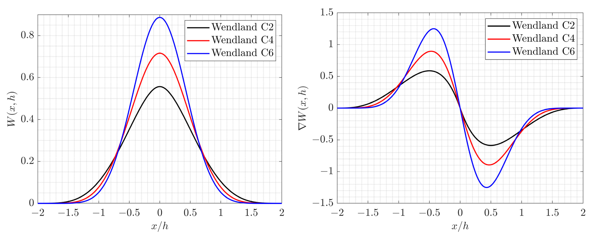
2.3. The Smoothing Kernel Functions

The kernel function, as pointed out before, plays a pivotal role in the formulation of the WCSPH numerical scheme. The use of one kernel for the density estimation and a different kernel for the pressure computation to get better results was suggested by Thomas and Couchman [40], but such an approach results in the violation of energy and entropy conservation. Dehnen and Aly [11] carried out investigations into the stability of kernel functions with respect to particle instability, and it was found out that the Wendland functions were the ideal kernel functions, especially at higher-neighbor numbers. The family of Wendland functions has a number of functions of increasing order, and three of them normalized for use in 2D will be used in the present study for comparisons in different simulation scenarios. Specifically, the kernels used in the present study are the 5th-degree class 2 kernel (WC2 from now on), the 8th-degree class 4 kernel (WC4 from now on) and the 11th-degree class 6 kernel (WC6 from now on). The kernel functions have been formulated to have a domain radius of $2h$, where $h$ is the smoothing radius. For all the simulations carried out in the present study, $h$ has been taken to be equal to 1.5$\Delta x$, where $\Delta x$ is equal to the inter-particle spacing. The kernel functions are given as follows.

$$W_2\left(r,h\right)=\left\{\begin{array}{c}{\alpha }_{d2}\left(2q+1\right){\left(1-\frac{q}{2}\right)}^4 for 0\le q\le 2\\ 0 for q>2 \end{array}\right. \mathrm{where}, {\alpha }_{d2}= \frac{7}{4\pi h^2}$$

(15)

$$W_4\left(r,h\right)=\left\{\begin{array}{c}{\alpha }_{d4}\left(\frac{35}{12}{q}^2+3q+1\right){\left(1-\frac{q}{2}\right)}^6 for 0\le q\le 2\\ 0 for q>2 \end{array}\right. \mathrm{where}, {\alpha }_{d4}= \frac{9}{4\pi h^2}$$

(16)

$$W_6\left(r,h\right)=\left\{\begin{array}{c}{\alpha }_{d6}\left(4q^3+\frac{25}{4}{q}^2+4q+1\right){\left(1-\frac{q}{2}\right)}^8 for 0\le q\le 2\\ 0 for q>2 \end{array}\right. \mathrm{where}, {\alpha }_{d6}= \frac{78}{28\pi h^2}$$

(17)

Here, $q=\frac{\left|r\right|}{h}$. Their derivatives read as

$$\nabla W_2\left(r,h\right)= \left\{\begin{array}{c}{\beta }_{d2}{\left(1-\frac{q}{2}\right)}^{3}q\frac{r}{\left|r\right|} for 0\le q\le 2\\ 0 for q>2\end{array}\right. \mathrm{where}, {\beta }_{d2}=-\frac{35}{4\pi h^3}$$

(18)

$$\nabla W_4\left(r,h\right)= \left\{\begin{array}{c}{\beta }_{d4}\left(70q+28\right){\left(1-\frac{q}{2}\right)}^{5}q\frac{r}{\left|r\right|} for 0\le q\le 2\\ 0 for q>2\end{array}\right. \mathrm{where}, {\beta }_{d4}=-\frac{3}{8\pi h^3}$$

(19)

$$\nabla W_6\left(r,h\right)= \left\{\begin{array}{c}{\beta }_{d6}\left(8q^2+7q+2\right){\left(1-\frac{q}{2}\right)}^{7}q\frac{r}{\left|r\right|} for 0\le q\le 2\\ 0 for q>2\end{array}\right. \mathrm{where}, {\beta }_{d6}=-\frac{858}{112\pi h^3}$$

(20)

Here, $r$ is the distance from the considered particle from its neighboring particles. The plots of the kernel functions and their gradients are provided for the purpose of visualization in Figure 1. As evident from this figure, with the increase in the order of the kernel function, the center peak value keeps increasing for the family of Wendland kernels. Moreover, the domain of influence keeps decreasing sharply for the Wendland kernels with increasing order. Thus, the Wendland C6 kernel has the particle itself significantly influencing the computation of its properties. This influence is found to decrease with the decrease in order of the kernel. Likewise, for the kernel gradient function, much more impetus is given to the nearby particles during the calculation, when kernels of higher orders are used. It can be seen that as the order of the kernel increases, the smoothing becomes less and less gradual.

2.4. Boundary Handling

The boundaries in the present study are based on the dynamic boundary condition [41]. The boundary particles follow the same set of equations as the fluid particles, with the only difference being that they are constrained not to move according to the forces. They either remain fixed or move according to some externally applied forces, exerting repulsive forces on particles that approach the boundary particles. With the absence of any explicit no-penetration boundary condition, the spacing between the boundary particles sometimes needs to be modified during different simulations for convergence. This approach has been chosen for its simple nature, with all of the computations becoming possible only with a single set of equations for all of the particles.

The numerical schemes are implemented by using CUDA 10.1 [42] to take advantage of the massively parallel nature of the computation, thereby saving a huge amount of computational time. Furthermore, the model is run by utilizing high-performance computing (HPC) facilities of the Bluecrab [43] cluster, specifically using the p100 GPU partition, which allowed multiple jobs to be run at the same time, saving much time in the process.

3. Validation Studies

Several numerical experiments were carried out to validate the different numerical dissipation schemes as well as compare the performance of the different Wendland kernels in simulation scenarios, which occur over a small domain for a short period of time involving impact against structures. Specifically, three scenarios were considered. The first is the common two-dimensional dam-break experiment. Pressure readings at a specified location were determined to compare with corresponding experimental readings for different Wendland kernels. The other simulation scenarios include the lateral and the roof sloshing experiments, the details of which are available on the SPHERIC [44,45,46,47] website. Like the dam-break problem, pressure measurements were determined at specific sensor locations used in the simulations, and the results were compared to the experimental findings.

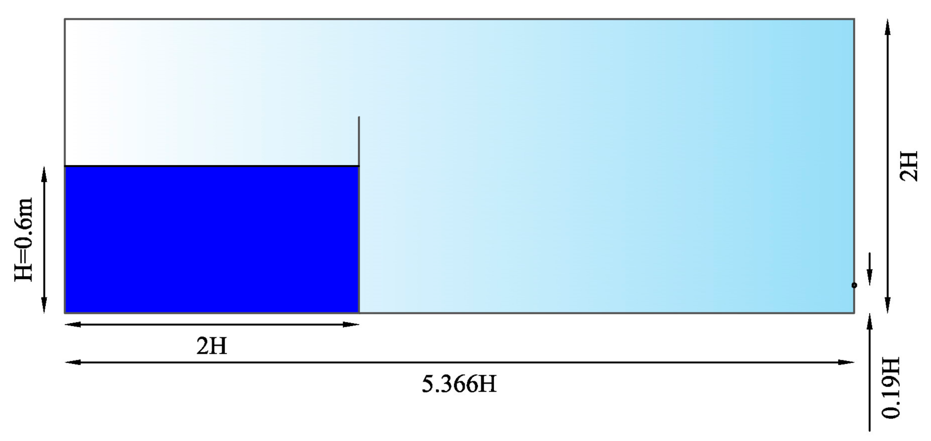
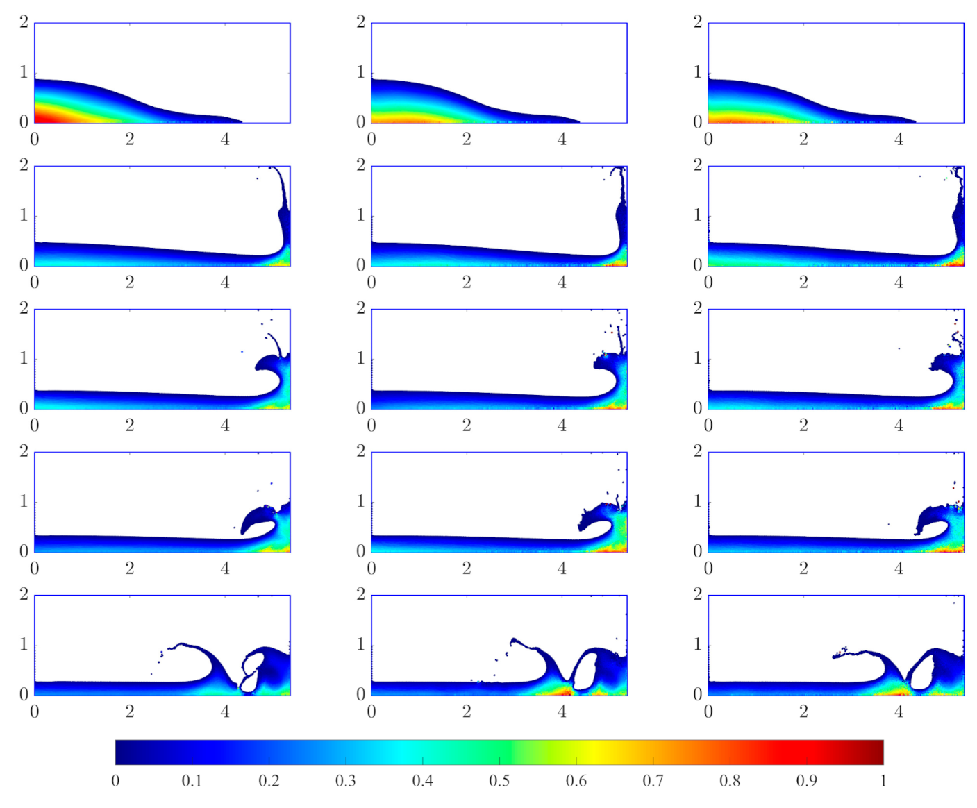
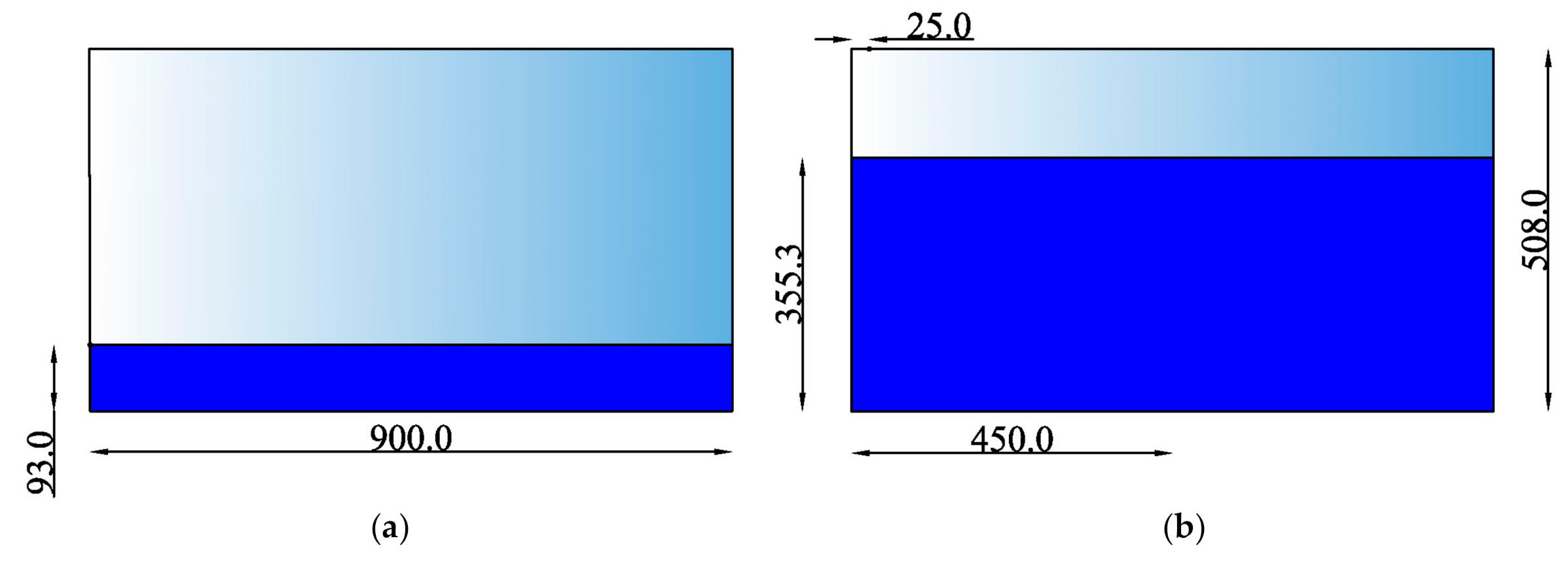
3.1. Dam-Break Simulations

The two-dimensional classic dam-break problem consists of a tank of width $W=5.366H$ with a fluid occupying a domain of width $W_F=2H$ and height $H=600 \mathrm{m}\mathrm{m}$ at the lower left end of the tank. The fluid column undergoes a simple hydrostatic initialization before the breaking of the dam is initiated. As the simulation starts, the fluid column collapses and moves towards the other wall where it undergoes an impact with the wall and settles down finally after crashing down as a plunging wave. An illustration of the set-up of the experiment is provided in Figure 2. The fluid properties and the parameters used during the simulations are summarized in

Table 1. Parameters and numerical setting used for the dam-break simulations.

$\mathbf{Fluid} \mathbf{Particle} \mathbf{Spacing} \left(\mathbf{\Delta }\mathit{x}\right)$	H/100
Boundary particle spacing	0.6$\Delta x$
Smoothing length $h$	1.5$\Delta x$
${\rho }_{ref}$	1000
Artificial viscosity coefficient $\alpha$	$\in \left[0,0.2\right]$
$\beta$ used in momentum equation	$\in \left[0,6.0\right]$
$\delta$—SPH coefficient	$\in \left[0,0.2\right]$
$v_{max}$	$\sqrt{gH}$
$c_0$	$20 v_{max}$
$\nu$ used in Morris viscosity factor	8.97 × 10−7

.

The simulation closely follows the simulation set-up used by Adami et al. [48] in their work about ghost-particle boundary implementation. The tank in the present scenario was kept closed (with a height of $2H$) to prevent particles from moving out of the simulation domain for lower computational costs. The pressure at a point on the far wall at a distance $0.19 H$ from the bottom was measured and compared against the results from an experiment [49]. As pointed out before in other studies [48,50], the wave probe used in the experiment was at a slightly different location, but following earlier validation studies [50], we decided to use the said location for pressure measurements.

The different numerical dissipation schemes were implemented in the simulations with the different kernel functions. With the use of WC4 kernel function, the obtained behavior with the different dissipation schemes is shown in Figure 3. The pressure at the desired location for the numerical simulation was computed using the basic equations of the SPH that read as follows.

$$P_i=\frac{{{\displaystyle \sum }}_j{P}_j{W}_{ij}}{{{\displaystyle \sum }}_j{W}_{ij}}$$

(21)

where $i$ is the particle location where the pressure is to be measured and $j$ is the neighboring particle. The location measurement is considered to be at a distance of 0.01$h$ from the sensor location on the right wall.

It can be seen from Figure 3 that, apart from the behavior with the artificial viscosity scheme, the behaviors with other numerical dissipation schemes are found to be quite similar. Significant pressure oscillations are observed with the artificial viscosity scheme, which is not the case with the other schemes. The density reinitialization scheme works the best as far as the hydrostatic pressure initialization is concerned, and the scheme that the authors ultimately made use of is a combination of the $\delta$-SPH scheme with the density reinitialization scheme along with the artificial viscosity term coefficients α and β for the best results. It needs to be noted here that the parameter β is found to play a significant role in the results obtained for the chosen scheme after sufficient tuning and also proved important for the stability of the scheme. Though the results agree to a significant extent with experimental observations, there are discernible deviations as well. The initial rise of pressure at around $t{\left(\frac{g}{H}\right)}^{0.5}=2.5$ as well as the pressure spike at around $t{\left(\frac{g}{H}\right)}^{0.5}=5.8$ in the experiments are observed to be delayed in the simulation results. This may be due to the modified location of the pressure probe leading to a phase difference. The high-frequency pressure oscillations in the simulations not seen in the experimental results are the result of the weakly compressible nature of the computational model itself; this results in a high amount of noise. Similar results were obtained when the other kernel functions were used with the above dissipation schemes. A grid study was carried out to investigate the convergence of the different dissipation schemes used for the dam break simulations. The results of this grid study are depicted through an L2 error plot in Figure 4, wherein the L2 errors have been computed for three different resolutions for each of the dissipation schemes and interpolated for other values within the range of these resolutions. The different particle resolutions used are $\frac{H}{100},\frac{H}{50}$, and $\frac{H}{25}$. The L2 error for a particular resolution has been computed using the formula

$$L_2=\sqrt{\left(\frac{1}{N}{\displaystyle \sum }_{i=1}^N{\left(P_{comp}\left(t_i\right)-P_{exp}\left(t_i\right)\right)}^2\right)}$$

(22)

where $N$ is the total number of observations at specific time instants over the course of the simulation, $t_i$ represents the time instants, $P_{comp}$ is the pressure computed numerically at our location of interest at a specific time instant using Equation (21), and $P_{exp}$ refers to the experimental results from reference [49]. The interpolation in the plot was carried out using the inbuilt MATLAB “fit” function, with which a smoothing spline model is utilized to fit the data. A smoothing parameter with values lying between 0 and 1.0 can be used in conjunction with this model type to determine the smoothness of the fit data, with a value of 1.0 meaning that the fit data coincide with the original data. A smoothing parameter of 0.995 was used for the present case. For purposes of comparison, the L2 errors were plotted on a logarithmic Y-scale against the inter-particle distance. The errors decrease with increasing resolution, thus showing that the schemes are convergent in nature when used for the dam break simulations. Lines showing the order of increase of the errors with increasing inter-particle distance have also been depicted for ease of visualization. It is evident from Figure 4 that the use of an artificial viscosity scheme results in the largest error throughout the range of the particle resolution used, increasing at a rate of 0.3rd order of the inter-particle distance. For the $\delta$—SPH scheme, the error decreases at a rate of 0.6th order of the inter-particle distance with increasing resolution, which is the highest observed amongst the different schemes used. The least error is observed for the density reinitialization and the chosen scheme, with the convergence rates being 0.18 and 0.02, respectively. Based on this, it can be stated that the chosen dissipation scheme is the most suitable for a wide range of particle resolutions when compared to the other schemes. However, the $\delta$—SPH scheme is expected to perform better at higher particle resolutions, since it has the highest convergence rate.

In Figure 5, the authors compare the pressure data obtained from the simulations by using the different kernels for the chosen dissipation scheme as described above against the experimental findings. In the scheme chosen for the comparison of the kernels, the authors combine the different dissipation schemes as discussed before, and the parameter β was tuned carefully for each of the kernel functions to arrive at a result that has considerable agreement with the experiment results. The time delay in the pressure rise and spike is similar for all the kernels. However, the magnitude of the pressure and the offset from the experimental observations are observed to be lesser for the WC4 and WC6 kernels compared to that with the WC2 kernel. The frequency oscillations are observed to be of less magnitude for the WC2 kernels compared to the other two. This leads to smoother surface profiles of fluid particles for simulations when using WC2 in comparison to WC4 and WC6. The pressure contour plots provided in Figure 5 help visualize these observations.

From the second, third and fourth rows of the pressure snapshots in Figure 6, it can be observed that the pressure at the location of interest remains higher in the case of the WC4 and WC6 kernel simulations compared to that obtained for the WC2 case. On the contrary, the surface profile for the wave crest is much smoother in the case of the WC2 simulation than for the WC4 and WC6 ones, as apparent from comparing the same subplots as above.

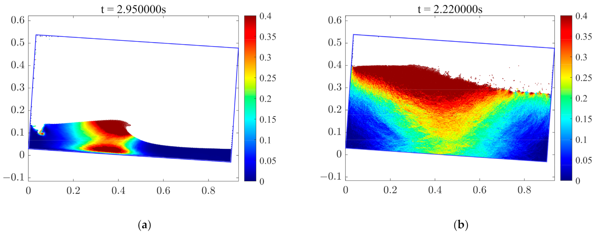
3.2. Sloshing Simulations

Two different scenarios involving lateral and roof impact in a rectangular tank were simulated to validate the results against the findings from experiments conducted by Souto-Iglesias and Botia-Vera. The details of the experiments can be found on the SPHERIC [44,45,46,47] website. The experiment consists of a rectangular tank with a width $W=900 \mathrm{m}\mathrm{m}$ and a height $H=508 \mathrm{m}\mathrm{m}$. For sloshing to take place, the tank is rotated about an axis that is fixed to the center of the bottom line of the tank. Pressure measurements were taken at specific locations with sensors attached to the tank walls. Three different tank widths were used during the actual experiment, but a two-dimensional case was considered for the numerical studies.

Two different tank filling levels were used. The filling level corresponding to 18% of the tank height (i.e., $93 \mathrm{m}\mathrm{m}$) was used for lateral sloshing with pressure to be measured at $93 \mathrm{m}\mathrm{m}$ from the bottom on the left wall of the tank. The period of the sloshing motion for this case was $1.919$ s. For simulation purposes, the real-time angle curves provided on the SPHERIC website were used. The filling level corresponding to 70% of the tank height (i.e., $355.3 \mathrm{m}\mathrm{m}$) was used for the roof sloshing experiment, with the resulting pressure being measured at $25 \mathrm{m}\mathrm{m}$ from the left wall at the top of the tank. A period of 1.167 s was used for the actual experiment, but again, the provided real-time angle curves were used for the simulations. An illustration of the set-up for the two different simulation scenarios is provided in Figure 7.

The two simulation scenarios with the different fluid levels correspond to different types of fluid motions. The lateral sloshing simulation with the low filling level involves irregular fluid motion with overturning waves while the roof sloshing simulation with the high filling level corresponds to fluid with high acceleration without any breaking waves. For better visualization, the obtained snapshots of the velocity profiles for the simulations are provided in Figure 8.

As was done in the dam-break problem, the different dissipation schemes were impleented with the different Wendland kernels to compare the simulation results against the experimental pressure readings. The fluid properties and the parameters used during the simulations for this numerical experiment are tabulated in

Table 2. Parameters and the numerical setting used in the sloshing simulations.

$\mathbf{Fluid} \mathbf{Particle} \mathbf{Spacing} \left(\mathbf{\Delta }\mathit{x}\right)$	W/450
Boundary particle spacing	0.6$\Delta x$
Smoothing length $h$	1.5$\Delta x$
${\rho }_{ref}$	998
Artificial viscosity coefficient $\alpha$	$\in \left[0,0.2\right]$
$\beta$ used in the momentum equation	$\in \left[0,4.5\right]$
$\delta$—SPH coefficient	$\in \left[0,0.3\right]$
$v_{max}$	$1.0$
$c_0$	$20 v_{max}$
$\nu$ used in Morris viscosity factor	8.97 × 10−7

.

As observed during the dam-break simulations, the artificial viscosity scheme when used alone with only the artificial viscosity coefficient α resulted in huge pressure oscillations during the lateral sloshing studies. Discernible differences in the pressure distribution at the measurement location during the time of impact were also observed among the other dissipation schemes. Similar to the dam-break simulations, a numerical dissipation scheme was created by utilizing the density reinitialization, the $\delta$—SPH coefficient and the artificial viscosity coefficients α and β. This scheme was implemented in addition to the other discussed schemes for the different kernels after a proper tuning of the parameters α, β and $\delta .$ The results were found to be in good agreement with the experimental readings. In Figure 9a, a comparison of the different dissipation schemes for the WC2 kernel for the lateral sloshing simulations is provided. In Figure 9b, the authors compare the results obtained with the implementation of the previously mentioned dissipation scheme for the different kernels with the corresponding experimental observations.

The implementation of the artificial viscosity scheme with the artificial viscosity coefficient α only has not been included in Figure 9a due to the high-magnitude pressure oscillations throughout the course of the simulation. These oscillations pose difficulties for the interpretation of the plot. The implementation of the $\delta$—SPH scheme alone results in a high second pressure spike just after the first, which was not observed during the physical experiment. The results obtained with the density reinitialization scheme closely resemble the experiment, with considerably less pressure fluctuations before and after the pressure spike. After using the density reinitialization along with the $\delta$—SPH scheme with properly tuned parameters α and β, the authors obtained a much better result in terms of agreement with the physical experimental readings. Similar to the dam-break simulations, the parameter β was found to play a significant role during the tuning process to arrive at the final results.

The dissipation scheme thus chosen was implemented with the different Wendland kernels. As evident from Figure 9b, the different Wendland kernels yield quite similar results when used with the abovementioned dissipation scheme, albeit with modified parameters within the range given in Table 2. However, some noticeable differences can also be observed. The pressure oscillations were the most frequent and of a higher magnitude with the WC6 implementation compared to the results obtained with the other kernels. The oscillations were the least for the WC2 kernel, as was the case during the dam-break experiments. The magnitude of the pressure spike was best captured with the help of the WC4 kernel, while the other kernels overestimated that by some margin. When compared with the physical experimental readings, a slight delay occurs in the formation of the pressure spike for all of the simulations. Furthermore, the presence of pressure oscillations, can be attributed to the weakly compressible nature of the numerical model.

Similar efforts were pursued for the roof sloshing simulations. The WC6 kernel was initially used for comparison among the different numerical dissipation schemes. This was followed by the comparison of the different kernels and the experimental readings using the finally adopted dissipation scheme. In Figure 10a, the authors give the comparison of the different dissipation schemes, and in Figure 10b, they compare the implementation of the adopted dissipation scheme amongst the different kernels with the experimental observations.

A similar behavior was observed from the implementation of the different numerical dissipation schemes, as was the case for the lateral sloshing simulations. As evident from Figure 10a, the artificial viscosity scheme resulted in large pressure oscillations during the time of impact, while the density reinitialization procedure was found to provide better results in terms of estimating the pressure spike magnitude with less pressure oscillations. The $\delta$—SPH scheme when used alone with the parameter $\delta$ did not converge for the range of $\delta$ mentioned in Table 2. The parameter β had to be added to the scheme for stability; however, a significant amount of pressure oscillations was still seen after the scheme was implemented. The scheme combining the density reinitialization, the $\delta$—SPH scheme with tuned artificial viscosity parameters α and β, showed the most agreement with the physical experiments, as was seen for the lateral sloshing simulations. This scheme was adopted for studying the kernel performance.

A similar trend was observed in the comparisons using the chosen scheme between the kernels and the experimental data. The WC6 and WC4 kernels were found to give very similar results that agreed well with the experimental data, with a stark difference observed towards the end of simulation duration. With the WC4 implementation, there were sudden pressure oscillations not observed in experimental data. The WC2 simulation results were found to resemble the experimental data the most, correctly capturing the pressure spike magnitude, unlike the overestimations observed with the WC4 and WC6 kernels.

4. Numerical Wave Tank Experiments

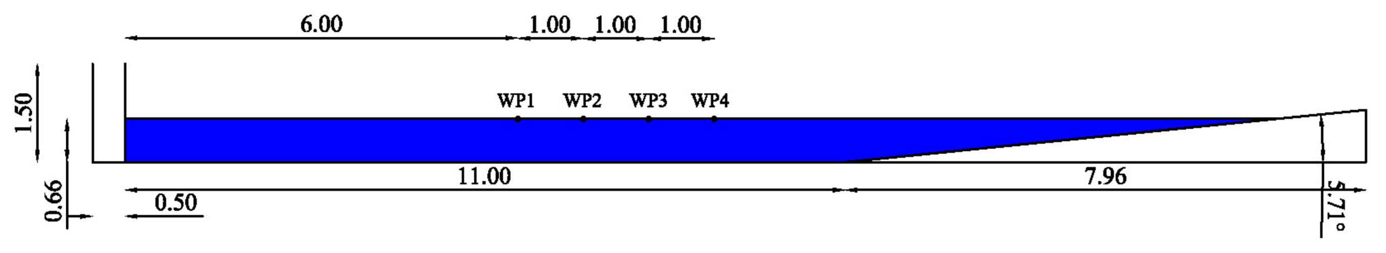
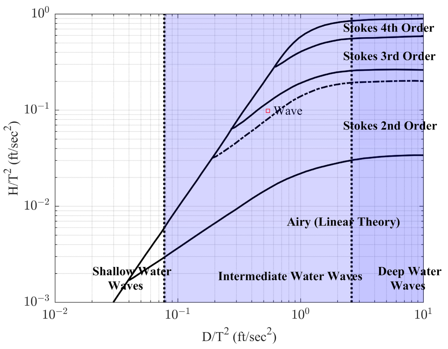
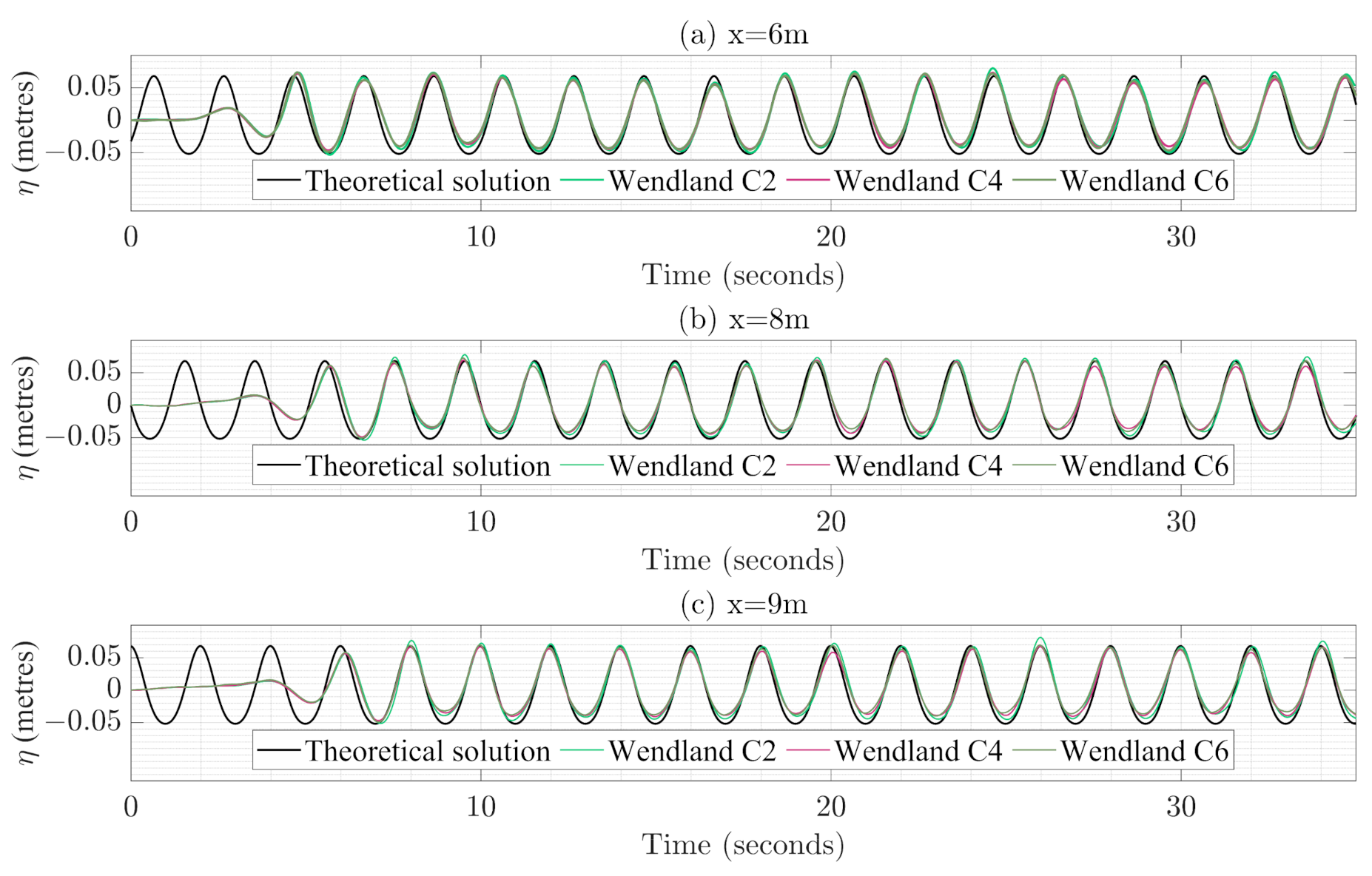
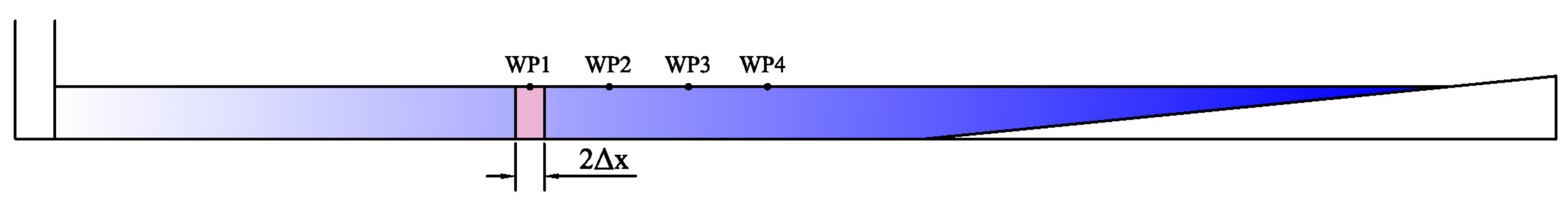
4.1. Wave Generation and Propagation

When one uses first-order wavemaker theory to generate regular waves in physical wave flumes, there is often the generation of unwanted secondary waves that influence the wave profile and height of the resultant waves as pointed out by Gōda [24] in 1967. This influence becomes more prominent with the increase in wave steepness $\left(H/L\right)$ ($H$ is the wave height and $L$ is the wavelength of the wave) or the decrease in relative depth $\left(d/L\right)(d$ is the water depth), with the waves generated not able to reach the predicted amplitudes. Second-order wave theory can be used to mitigate this problem and produce waves without spurious secondary wave components. The numerical simulations in the present study were carried out by implementing a second-order wavemaker theory with a piston-type wavemaker for intermediate water depth, a practical and common scenario in coastal engineering applications. The simple second-order wavemaker theory put forward by Madsen [25] and later improved on by Hughes [51] can be used to compute the displacement for a piston-type wavemaker to generate second-order Stokes waves. The equation for the same is given as follows:

$$s\left(t\right)= \frac{S_0}{2}\sin \left(\omega t+\delta \right)+\left[\left(\frac{H^2}{32d}\right)\left\{\frac{3\cos \mathrm{h}\left(kd\right)}{sin{h}^3\left(kd\right)}- \frac{2}{m_1}\right\}\right]\sin \left(2\omega t+2\delta \right)$$

(23)

where $s\left(t\right)$ is the wavemaker displacement, $S_0$ is the piston stroke length, $\omega =2\pi /T$ is the angular frequency where $T$ is the time period, $\delta$ is the initial phase which can vary from 0 and $2\pi$, $H$ is the wave height, $d$ is the water depth, $k=$ $2\pi /L$ is the wave number where $L$ is the wavelength and $m_1$ is the Biesel transfer function for a piston type wavemaker, which is expressed as follows:

$$m_1=\frac{H}{S_0}=\frac{2 sin{h}^2\left(kd\right)}{\sinh \left(kd\right)\cos \left(kd\right)+kd}$$

(24)

Schaffer [23] introduced a non-linearity parameter $S$, wherein for $S\ge 1$, second-order Stokes theory fails to predict the second-order harmonics correctly in a wave group. For a regular wave with angular frequency $\omega$, wavenumber $k$ and wave height $H$, the non-linearity parameter $S$ is given by:

$$S=2H\left|\frac{\omega H^{+}}{2g^{2}ktanh\left(2kd\right)-4g{\omega }^2}-\frac{1}{4g}\left(\frac{g^2{k}^2}{{\omega }^2}-3{\omega }^2\right)\right|$$

(25)

where $H^{+}$ is given by

$$H^{+}=2\omega \left({\omega }^2-\frac{g^2{k}^2}{{\omega }^2}\right)+{\omega }^3-\frac{g^2{k}^2}{\omega }$$

(26)

The wave conditions described in

Table 3. Wave conditions for the monochromatic wave used in the simulations.

Height H	0.12 m
Depth d	0.66 m
Wavelength L	4.52 m
Time Period T	2 s
Initial phase δ	0
Steepness s	0.026
Relative depth	0.146

correspond to a value of 0.5451 for the non-linearity parameter $S$. Hence, the wavemaker theory describing the 2nd-order Stokes waves is considered to be valid for the above wave conditions.

The simulation setup closely follows that of Altomare et al. [26], where passive absorption is provided at the end of the numerical setup to carry out long-duration wave simulations with much less reflection than for a fully rectangular tank. For the simulations used in the present study, the passive absorption was carried out through the addition of a long dissipative beach at the end of the rectangular part of the wave tank, where the wave energy dissipates due to the breaking of waves. The implementation of such a feature is advantageous as it requires no other modification to the existing code with a moderate increase in the size of the simulation domain. The simulation domain used for the current work consisted of a rectangular tank of width $11.5 \mathrm{m}$ with a dissipative beach having a slope of $5.71°$ at the end of the rectangular part, making the total length of the simulation domain equal to $19.46 \mathrm{m}$. The wavemaker was located at a distance of $0.5 \mathrm{m}$ from the left wall of the tank, and a water bed of depth $0.66 \mathrm{m}$ stretched from the right of the wavemaker to the end of the simulation domain. Four wave probes, denoted as WP1, WP2, WP3 and WP4, were put at distances of $6 \mathrm{m}$, $7 m, 8 \mathrm{m}$ and $9 \mathrm{m}$ from the initial wavemaker position to measure the surface wave elevation at the respective positions. The setup of the numerical wave tank is illustrated in Figure 11.

The wave experiments were carried out using monochromatic waves with the wave properties listed in Table 3. The wave conditions in Table 3 were chosen in a manner such that the monochromatic wave generated from the wavemaker motion corresponding to these conditions represent a second-order Stokes wave in the intermediate depth range, verified using the Le Mehaute abacus, as depicted in Figure 12.

Similar to the validation experiments carried out previously, the different dissipation schemes were implemented for the three Wendland kernels during the numerical wave tank experiments to compare the results. The fluid properties and the simulation parameters used during the course of the experiments are tabulated in

Table 4. Parameters and the numerical setting used for the numerical wave tank conditions.

$\mathbf{Fluid} \mathbf{Particle} \mathbf{Spacing} \left(\mathbf{\Delta }\mathit{x}\right)$	$\in \left\{2\times {10}^{-2} \mathbf{m}, 1.5\times {10}^{-2} \mathbf{m},1\times {10}^{-2} \mathbf{m},5\times {10}^{-3} \mathbf{m}\right\}$
Boundary particle spacing	$\in \left\{0.7\Delta x, 0.5\Delta x\right\}$
Smoothing length $h$	$1.5\Delta x$
${\rho }_{ref}$	1000
Artificial viscosity coefficient $\alpha$	$\in \left[0,0.01\right]$
$\beta$ used in momentum equation	$\in \left[0,2.0\right]$
$\delta$—SPH coefficient	$\in \left[0,0.1\right]$
$v_{max}$	$3.0$
$c_0$	$10 v_{max}$
$\nu$ used in Morris viscosity factor	8.97 × 10−7
Time step (Fixed time integration)	$1\times {10}^{-5} \mathrm{s}$

. As can be seen from Table 4, different values of fluid particle spacing were used to study the behavior of the kernels with decreasing grid spacing by comparing the wave elevations at the locations of the four wave probes. It was found that with a boundary particle spacing of $0.7\Delta x$ for implementations with the WC4 and WC6 kernels, the authors were able to prevent the fluid particles from going out of the simulation domain through the boundaries, but they were unable to do so with the WC2 kernel. Hence, a finer boundary particle spacing of $0.5\Delta x$ had to be used to prevent the penetration of the boundary particles with the WC2 kernel.

4.2. Results and Discussion

4.2.1. Hydrostatic Pressure Initialization

During the numerical wave tank experiments, the wave maker motion was imposed on the fluid particles after $5$ s of stationary time to allow the fluid particles to settle down. The hydrostatic pressure at the bottom of the numerical tank after the end of the initialization was calculated for the three kernel functions and compared with the analytical solution. The particle spacing used for the simulations carried out was $5\times {10}^{-3}\mathrm{m}$. The analytical pressure value at the bottom of the tank was $6.4746\times {10}^3 \mathrm{P}\mathrm{a}$. While the relative error in the computed pressure value and the analytical solution for the WC2 kernel was found to be $21.4\%$, those for the WC4 and WC6 kernels were calculated to be $15.2\%$ and $10.4\%,$ respectively. The higher error for the WC2 kernel could be due to the finer boundary particle spacing used during the simulation. However, the lower error obtained with the WC6 kernel compared to that with the WC4 kernel implies that, with the WC6 kernel, one obtains a better approximation of the hydrostatic pressure profile at the end of hydrostatic initialization in numerical wave tank experiments.

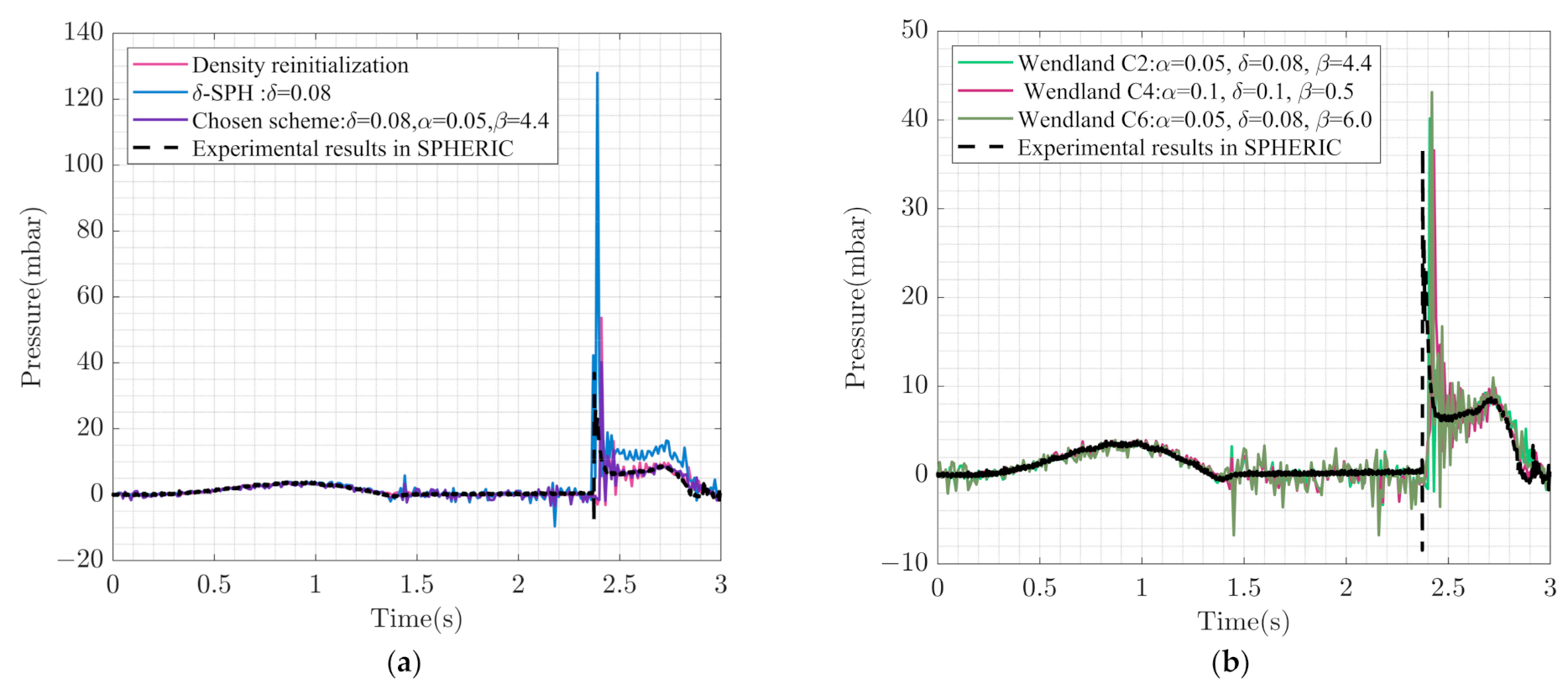
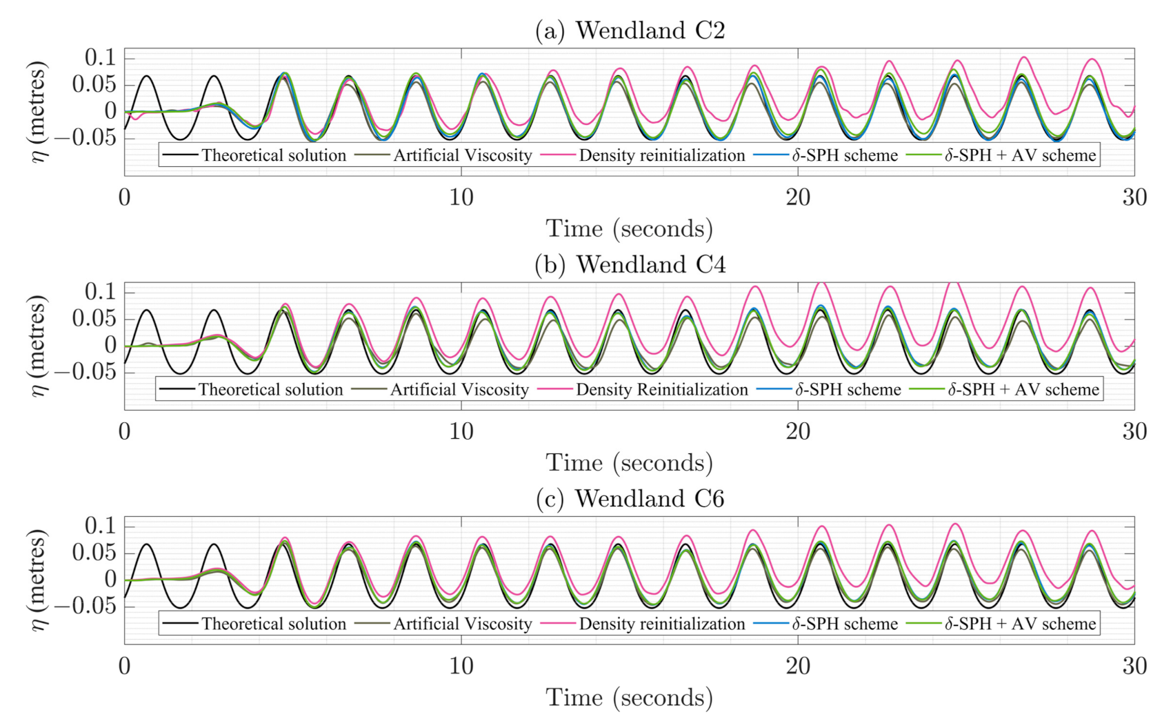
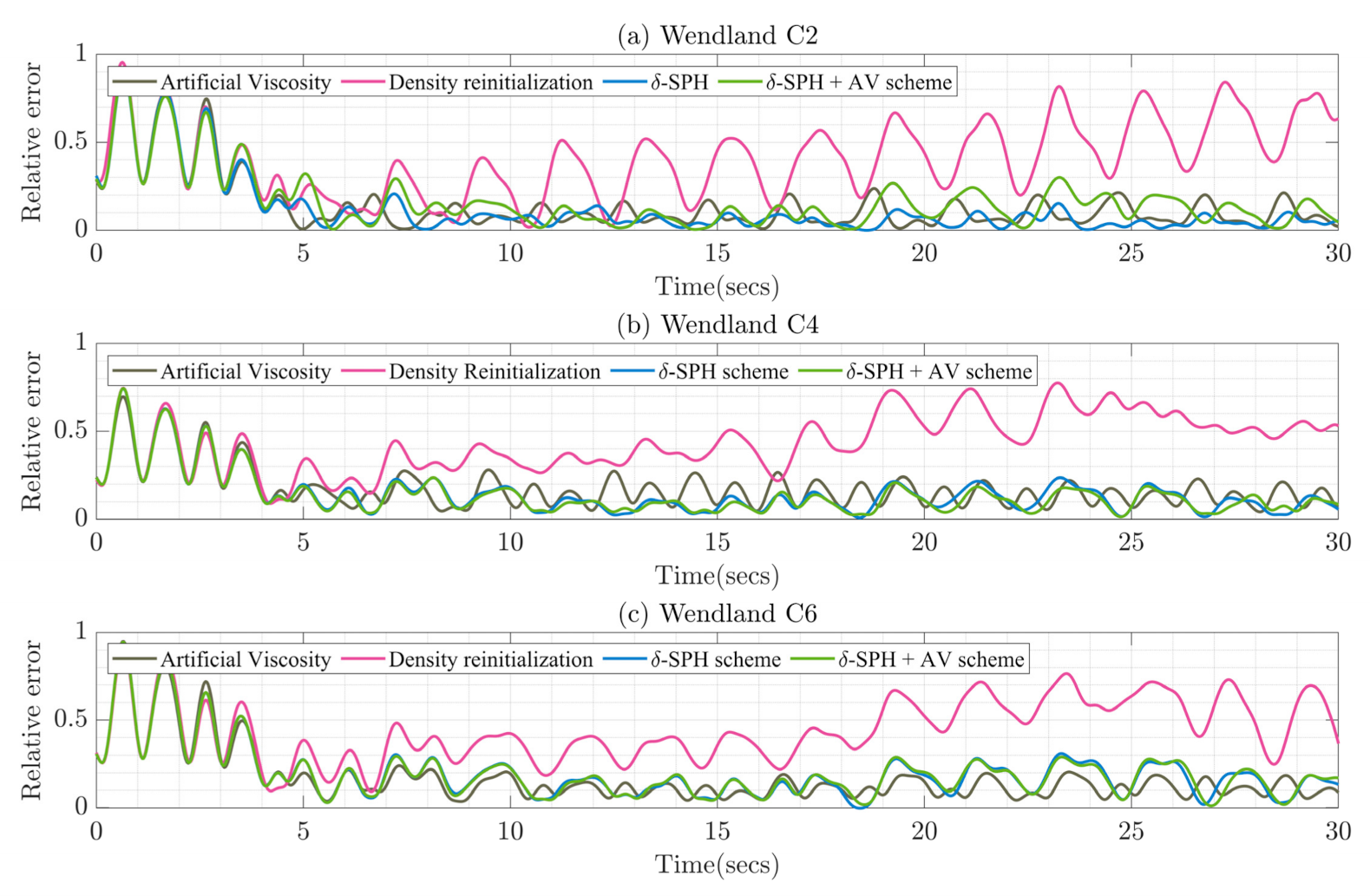
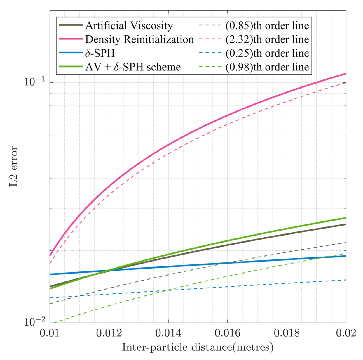
4.2.2. Comparisons with Different Dissipation Schemes

The different numerical dissipation schemes were implemented in the numerical model to see their suitability in capturing the wave surface elevation accurately. The comparisons were carried out between the elevations found out numerically and the wave elevation predicted by Stokes’ second-order wave theory [53] given as follows:

$$\eta \left(x,t\right)=a\left\{\cos \left(kx-\omega t\right)+ka\frac{3-tan{h}^2\left(kd\right)}{4tan{h}^3\left(kd\right)}\cos 2\left(kx-\omega t\right)\right\}$$

(27)

where $a$ is the wave amplitude and all other symbols have their usual meanings. Unless otherwise specified, the $\delta$–SPH coefficient when used in the numerical experiments was assumed to have a value of 0.05. For the WC2 kernel, the simulation became unstable when the density reinitialization procedure was used alone; however, implementing it with $\delta$-SPH yielded acceptable results. For all of the kernels, when implementing the artificial viscosity scheme alone, a minimum value of $\alpha =0.01$ was required for numerical stability. Since $\alpha$ is associated with the addition of dissipation in the simulations, this was always found to result in lower valued approximations than the theoretical predictions according to Equation (27). Lower values of $\alpha$ could have provided better approximations, but it was not possible because of the aforementioned numerical instability. As done previously, numerical experiments were also carried out by combining the above dissipation schemes. The comparisons of the wave elevations at the wave probe located at $x=6 \mathrm{m}$ for the different dissipation schemes obtained with the different kernels are given in Figure 13.

For better visualization of the results obtained, the corresponding errors with the theoretical predictions at $x=6 \mathrm{m}$ over 30 s of the simulation duration are also provided in Figure 14. For a better understanding, the relative errors are used for the plots, wherein the relative errors are computed as the absolute error divided by the maximum error observed for a particular kernel function during the numerical experiments.

The particle spacing used for the simulation results depicted in Figure 13 and Figure 14 is $1\times {10}^{-2} \mathrm{m}$. From Figure 13, it can be clearly seen that the density reinitialization scheme is not suitable for numerical wave tank simulations of large domains over long periods of time. The fluid particle spacing becomes unphysically high towards the surface with the progress of simulation, resulting in an increase in the fluid surface level, thus rendering the surface elevation observations inaccurate. With the other dissipation schemes, one observes similar behavior with respect to the elevation results, with only minor noticeable differences. The artificial viscosity coefficient helps incorporate dissipation into the system as pointed out before, and this induces some extra error as noticeable from Figure 14 for the WC2 simulations, where both the artificial viscosity scheme and the combination of $\delta$-SPH and artificial viscosity with $\alpha$ being 0.00001 results in a larger error margin compared to the $\delta$-SPH scheme implementation alone. A similar result to that obtained with the WC2 kernel was observed when the density reinitialization procedure was implemented for the WC4 kernel function with the surface elevation becoming increasingly unphysical as the simulation unfolded. The simulations returned similar errors for the other dissipation schemes with very little differences in the case of the WC4 kernel. As was noticed for the WC2 kernel, the density reinitialization did not lead to meaningful results for the WC6 kernel, with increasing fluid surface level over time. $\alpha$ was taken as equal to 0.00001 when used in the $\delta$-SPH scheme. The errors obtained for the other implemented schemes were found to be larger than those obtained with the WC2 simulations, with no noticeable differences amongst the error magnitudes for the various dissipation schemes. The WC6 and WC4 kernels thus seem more robust than the WC2 kernel with respect to the implementation of these dissipation schemes, when wave surface elevation measurements are concerned. On the other hand, when accuracy is of interest, the WC2 kernel results are found to be the best when the $\delta$-SPH scheme is implemented. Henceforth, for all future comparisons among the kernels, the results from the implementation of the $\delta$-SPH scheme were considered.

Based on observing similar behavior of the Wendland kernels with regard to the implementation of the different dissipation schemes, a representative grid study was carried out by using one of the kernel functions to investigate the convergence characteristics of the different numerical dissipation schemes. The WC6 kernel was chosen for this purpose, and the grid resolutions used for the purpose of the investigation were $2\times {10}^{-2}m, 1.5\times {10}^{-2}m$ and $1\times {10}^{-2}m$. The wave elevation at $x=6\mathrm{m}$ was extracted for the different cases and compared with the analytical solution. The location was chosen since it is sufficiently away from the ends of the wave tank. Thus, there are negligible effects of wave reflection to be anticipated in the results. The L2 errors for the different resolutions were computed for the different resolutions and then interpolated over the range of the particle resolutions chosen by using the MATLAB “fit” function with a smoothing parameter magnitude of 0.995. The L2 error is computed using the formula

$$L_2=\sqrt{\left(\frac{1}{N}{\displaystyle \sum }_{i=1}^N{\left({\eta }_{comp}\left(6,t_i\right)-{\eta }_{theo}\left(6,t_i\right)\right)}^2\right)}$$

(28)

where $N$ is the total number of observations at specific time instants over the course of the simulation, $t_i$ represents the time instants, ${\eta }_{comp}$ is the wave elevation computed numerically, and ${\eta }_{theo}$ is the wave elevation according to Equation (27). It is evident from Figure 15 that the different numerical dissipation schemes exhibit convergence when used for wave tank experiments, as the errors decrease with increasing grid resolution. It is observed that the implementation of the density reinitialization scheme results in the maximum error over the range of the particle resolutions chosen. However, the convergence rate observed for this is also the maximum, with the errors increasing at the 2.32nd order of resolution with increasing inter-particle distance. The $\delta$-SPH scheme implementation results in the lowest error at lower particle resolutions and associated with it is the lowest convergence rate of 0.25. The artificial viscosity scheme and the combination of artificial viscosity and $\delta$-SPH schemes behave quite similarly with convergence rates of 0.85 and 0.98, respectively, with the lower L2 error observed at the highest resolution than the $\delta$-SPH scheme. From the results depicted in Figure 15, it is expected that a similar trend would be observed for the WC2 and WC4 kernels, with minor differences in the convergence rates of the different numerical dissipation schemes.

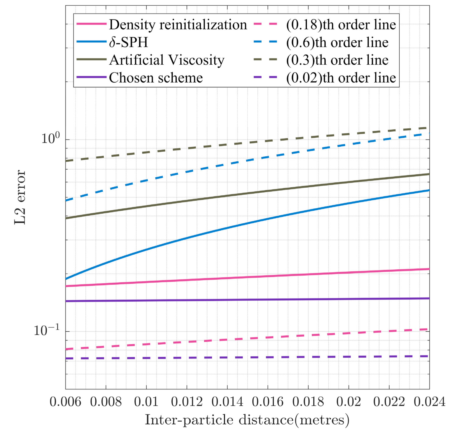
4.2.3. Particle Resolution Study

The $\delta$-SPH scheme chosen for further experiments was implemented for the different kernels using the four values of the particle spacing given in Table 4. The purpose of this was to study the behavior with the different kernel functions with respect to different particle resolutions used in the simulations. Similar to the previous study, the wave elevation at the location of $x=6\mathrm{m}$ was used for comparison with the theoretical solution. The observations at the said location for the simulations run with the three kernels for the time window of 10 to 12 s are provided in Figure 16a. The computed L2 errors for the different kernel function implementations over the different particle resolutions are given in

Table 5. Computed L2 errors for the particle resolution study using the different kernel functions.

$\mathbf{Fluid} \mathbf{Particle} \mathbf{Spacing} (\mathbf{\Delta }\mathit{x}\mathbf{)}$	$\left\{2\times {10}^{-2} \mathbf{m}, 1.5\times {10}^{-2} \mathbf{m},1\times {10}^{-2} \mathbf{m},5\times {10}^{-3} \mathbf{m}\right\}$
Wendland C2 errors	{0.0176, 0.0162, 0.0156, 0.0155}
Wendland C4 errors	{0.0177, 0.0155, 0.0160, 0.0156}
Wendland C6 errors	{0.0195, 0.0165, 0.0164, 0.0159}

.

In Figure 16b, the authors provide a better visualization of the above grid study by computing the L2 errors for the different resolutions for the three kernels and interpolating them over the range of grid resolution used. As observed from both Figure 16a and the observations tabulated in Table 5, the WC2 kernel is found to have the best agreement with the theoretical findings generally over the range of the particle resolution used. The L2 error plot given in Figure 16b aids in the visualization of this finding. The interpolation in this plot was carried out through the MATLAB “fit” function with a smoothing parameter magnitude of 0.995. For purposes of comparison, the logarithm of the errors was plotted against the inter-particle distance. The errors decreased with the increase in resolution for the different kernels, as expected. Lines depicting the order of increase of errors with the increase in resolution have also been provided. As evident from the plot, the error increases most sharply with increasing inter-particle distance for the WC6 kernel, corresponding to a 0.14th order line. The increase in error with a decrease in resolution is the most gradual for the WC4 kernel, corresponding to a 0.08th order line, while for the WC2 kernel, the error increases at a rate of 0.09th order of the inter-particle distance. The error is observed to be the least for the WC2 kernel at the highest resolution, while it is the least for the WC4 kernel at the highest inter-particle distance. An increase in resolution might achieve better results with the WC6 kernel; however, the increase in computational cost outweighs the improvements in results obtained.

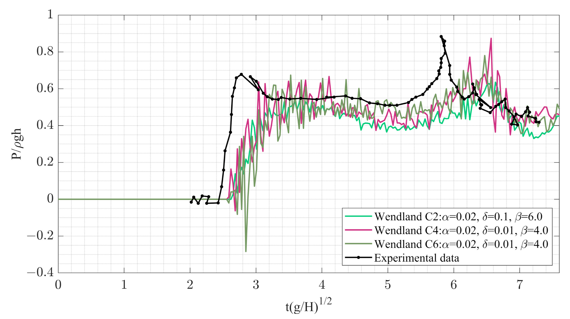
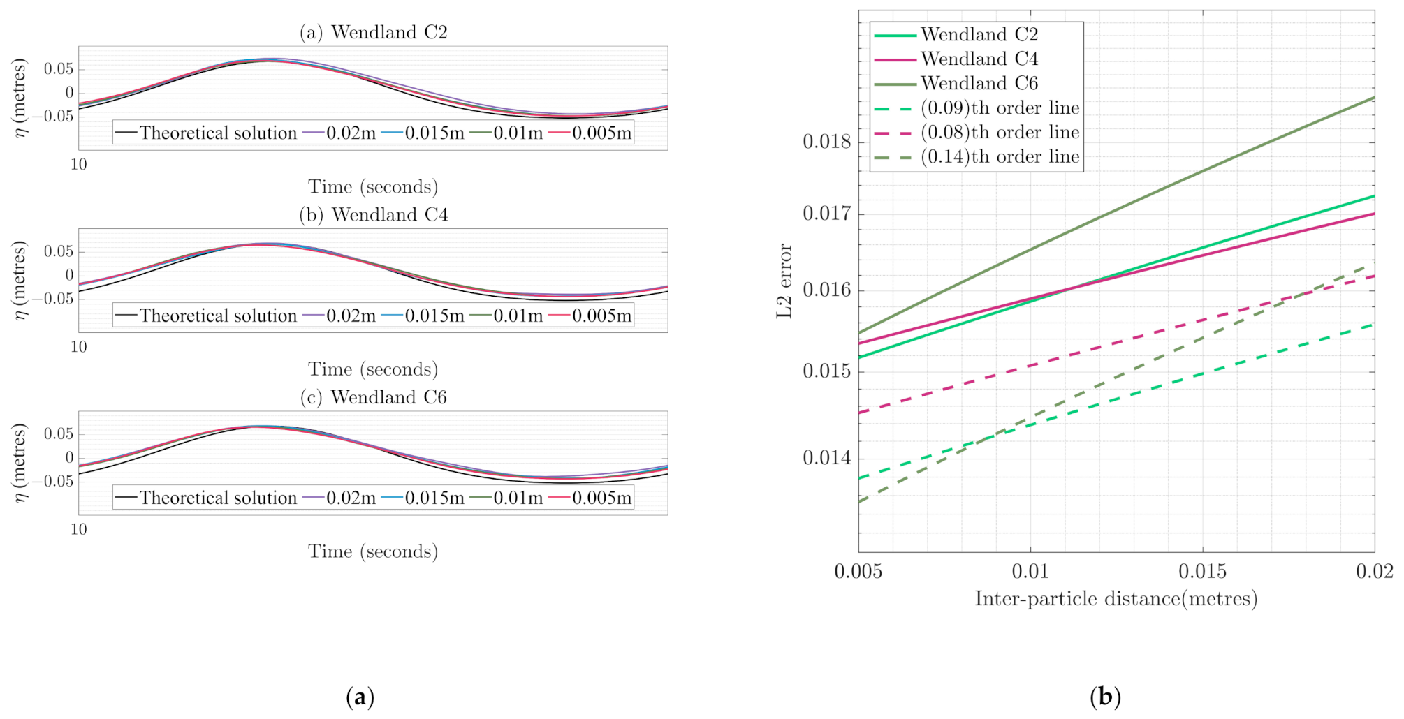
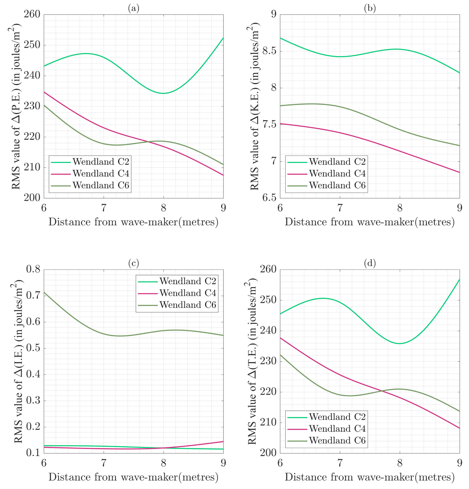
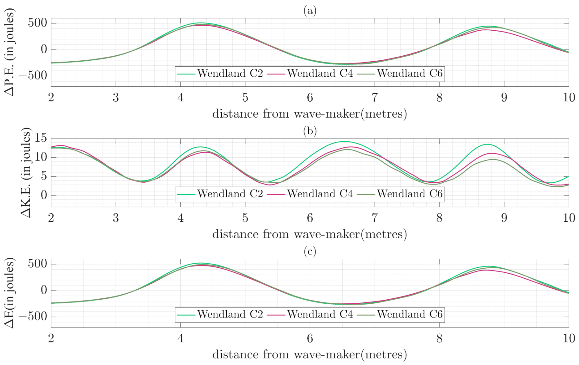
4.2.4. Effect of Kernels on Numerical Dissipation

Numerical dissipation is an intrinsic aspect of the WCSPH model due to the dissipation schemes that are included in the model for numerical stability. However, this becomes a problem for simulations of progressive waves that can travel over a large distance in a numerical wave tank with discernible wave structure throughout. Through the simulations conducted here, it was investigated if the kernel function itself has any discernible effect on being able to resist numerical dissipation in a numerical wave tank. To realize this, wave elevations were determined at the locations of the four wave probes and compared with the theoretical solutions. The comparison of the wave elevations at the three of the probe locations at $x=6 \mathrm{m}, x=8\mathrm{m}$ and $x=9 \mathrm{m}$ are given in Figure 17.

The plots shown in Figure 17 reveal that for all the kernels, the errors between the theoretical predictions and the numerical computations of the wave surface elevation increase gradually with increasing distance from the wavemaker, especially, in being unable to capture the troughs of the surface profile accurately. However, the behaviors with each of the kernels are found to be quite similar, and one cannot differentiate one from the other in these plots.

Since dissipation means loss of energy in a system, post-processing calculations were carried out to aid in better visualization of the numerical dissipation effect for the different kernel functions using the results generated for Figure 17. The particle spacing used for the simulations in this case is $5\times {10}^{-3}\mathrm{m}$. For this, the energy change per unit area at the wave probe locations was calculated by assuming that the total energy comprised potential energy, kinetic energy and the internal energy of the fluid particles. The different energy terms are calculated as follows.

$$E_{int}= \frac{m_p{\rho }_0}{{\rho }_0\left(\gamma -1\right)}\left({\left(\frac{{\rho }_t}{{\rho }_0}\right)}^{\gamma -1}+ \frac{{\rho }_0}{{\rho }_t}\left(\gamma -1\right)-\gamma \right)+ E_{int}\left({\rho }_0\right)$$

(29)

$$E_{kin}= m_p\frac{{v_p}^2}{2}$$

(30)

$$E_{pot}= m_{p}g{y}_p$$

(31)

where $m_p$ is the mass of each particle, ${\rho }_t$ is the density of the particle at time $t$, ${\rho }_0$ is the reference density,$v_p$ is the velocity of particles and $y_p$ is the height of the particle above the tank base.

Equation (29) is used to calculate the change in internal energy of each particle [50], while Equations (30) and (31) are used to calculate the kinetic energy and potential energy of each fluid particle. For computation, a strip of length of $2\Delta x$ around the wave location is used, where $\Delta x$is the particle spacing and the energies of all the particles lying within the strip are calculated and summed up and finally divided by $2\Delta x$ to give the total energy per unit area at the location at a particular time. This was calculated for the entire simulation duration at the wave probe locations for all the experiments carried out to obtain the results shown in Figure 16. An illustration of the working method is provided in Figure 18 for clarification. The wave probe locations from $x=6 \mathrm{m}$ to $x=9 \mathrm{m}$ were chosen for this study as the effect of wave reflection is minimum in this central part of the numerical tank.

Following the computations of the different energies using the process and equations mentioned, a time series is obtained for each of the energy quantities. To gauge the numerical dissipation effect on each kernel function, an average value of each of the quantities at the different locations was found out by using the RMS value of the observations as follows:

$$Q= \sqrt{\frac{1}{N}{\displaystyle \sum }_{i=1}^{N}y{\left(t_i\right)}^2}$$

(32)

where $Q$ is the average value of the energy quantity under consideration, $N$ is the number of time observations, and $y\left(t_i\right)$ are the computed values of the different energy quantities at different time instants. $N$ has been taken equal to 875 for the experiments carried out above. The plots depicting the RMS values of the energy quantities at the wave probe locations are given in Figure 19. The intermediate values between the actual locations have been interpolated using the MATLAB “fit” function with a smoothing parameter magnitude of 0.995 as done before.

It is the evident from the plots in Figure 19 that the potential energy change accounts for the bulk of the total energy, with relatively small contributions from the kinetic energy and internal energy changes during the simulation. From the plots, it is clear that the potential energy continues to decrease gradually for the WC4 and WC6 kernels with the increase in distance from the wavemaker, with no oscillating nature detected. With the RMS average potential energy for the WC2 kernel, one sees an oscillatory pattern for the range of distances with no continuous decay of energy observed. The kinetic energy RMS value for the WC2 kernel also is higher than those obtained with the other two kernels, signifying that the particle velocities remain higher during the WC2 kernel simulations than during the WC4 or WC6 simulations, with the loss of energy also slightly lower at this distance. The internal energy RMS value is found to remain fairly constant throughout the simulations for the WC2 and WC4 kernels, while it drops by a very small amount for the WC6 kernel. Overall, the total energy RMS value is found to follow the trend observed with the potential energy, signifying that the WC2 kernel gives the best option against the effect of numerical dissipation for long-range numerical wave tank simulations. To look at a possible explanation for the observations above, the kernel functions and gradients are investigated closely. The energy calculations involve the velocities and positions of the particles, which are calculated from the particle accelerations. The calculation of the acceleration, as seen from Equation (5), depends on the kernel gradient as well as the function itself. The shape of these function plots is indicative of the behavior of these kernel functions. For the higher-order kernel functions with sharper profiles, there is a greater influence of the particles in the immediate vicinity of the particle under consideration when calculating the velocities and positions. For the lower-order kernels with more flattened profiles, the neighbors far away also have considerable influence on the calculation of a particle’s properties. This helps in achieving better smoothing of the properties, and thus, when averaged over particles within a certain span of distance, the calculation of energy is better smoothed out, with lower fluctuations over time and possibly better conservation.

To better consolidate this observation, the potential energy, kinetic energy and the total energy quantities were computed over a considerable portion of the wave tank at a particular time instant using the procedure discussed above. The internal energy was not included since it only accounted for a negligible amount of the total energy change. The different plots with the comparisons of the energy profiles among the kernels from $x=2 \mathrm{m}$ to $x=10 \mathrm{m}$ of the wave tank are given in Figure 20.

To generate the results of the above plots, the time chosen was $t=20$ s. The potential energy profiles for the three kernel functions were very similar at this particular time instant, but the kinetic energies of particles started decaying towards the end of the tank for the WC4 and WC6 kernels. This results in a loss of the total energy due to numerical dissipation in a more pronounced manner compared to the WC2 kernel.

5. Variation of Parameters in WCSPH Simulations

The weakly compressible nature of the WCSPH numerical scheme results in spurious density fluctuations over the course of a simulation. As pointed out before, numerical dissipation schemes were devised to dissipate these pressure oscillations to help render realistic simulations. These numerical schemes involve a number of parameters, which need to be modified according to the simulation scenario for the required numerical stability and a desired level of accuracy. The dissipation schemes implemented in the different simulations throughout the present work involve a host of parameters that had to be tuned based on the simulation conditions to get realistic results. These include the artificial viscosity coefficient $\alpha$, the coefficient $\beta$ used in the momentum equation, the $\delta$—SPH coefficient and the speed of sound $c_0$, which depends on the maximum fluid velocity $v_{max}$. The smoothing length $h$ was varied between $1.3 \Delta x$ and $1.5 \Delta x$, and finally, a value of $1.5 \Delta x$ was used for the different simulations. A larger value of the smoothing length is often found to lead to a tensile instability, and hence, this was avoided. On the other hand, for a lower value, not enough neighbors are involved for accurate calculations.

The coefficient $\alpha$ depends on the size of the simulation domain and the particle resolution used. The smaller the simulation domain and the number of particles used, the larger the value of $\alpha$ that is required for numerical stability. For the dam break simulations, when used alone, a value of $\alpha$ greater than at least 0.1 is required for numerical stability. However, when used with other parameters like $\beta$ or $\delta$, smaller values like 0.02 can help achieve the required stability. When $\alpha >0.2$ is used, larger viscous forces are generated, leading to excessive dissipation that renders the simulation impractical. For sloshing simulations, a similar trend is observed. For $\alpha$ in the range of 0.08–0.2, stable solutions are realized when implemented separately. However, with higher values of $\alpha$, excessive damping is observed. For the wave tank simulations that involve a larger domain and a much greater number of particles, with a smaller value of $\alpha =0.01,$ one can obtain stable solutions. However, the damping involved does not allow for a desirable degree of accuracy in the results. When implemented with other dissipation schemes, a value of $\alpha =0.00001$ can help achieve more accurate results.

The coefficient $\beta$ plays an important role in achieving numerical stability and accuracy, especially when pressure measurement is concerned. For the dam break simulations, a value of $\beta =2.0$ helps achieve numerical stability, even when values of $\alpha$ lower than 0.1 are used. Values of $\beta$ in the range of 3.0–4.0 can help achieve accurate results for the WC4 and the WC6 kernels as far as the dam break simulations are concerned, while a value in the range of 6.0–7.0 leads to sufficiently accurate results for the WC2 kernel. In general, for larger values of $\beta ,$the result is larger repulsive forces, and this can help prevent particles from penetrating the domain boundaries, aiding in achieving numerical stability. For the sloshing simulations, values of $\beta$ lying between 4.0 and 6.0 help in realizing accurate results. The effect of $\beta$ is less profound in large simulation domains like the wave tank simulations. However, this parameter can still be quite effective in imparting stability to schemes at lower values of $\alpha$ and $\delta$, thus reducing excessive damping, thereby helping to achieve realistic results. A value of $\beta$ in the range 2.0–4.0 can help achieve stability when the density reinitialization scheme is implemented in the wave tank simulations.

The $\delta$—SPH coefficient has been varied between 0.02 and 0.1 for the different simulations carried out as part of the current work. Values of $\delta$ greater than 0.2 result in excessive damping as was observed with the coefficient $\alpha$. Accurate results for the dam break simulations were obtained for $\delta$ values between 0.02 and 0.08 when used with the other artificial viscosity parameters. On the other hand, for the sloshing simulations, the $\delta$ values were observed to be between 0.08 and 0.1. For the wave tank simulations with a large domain size, a value of $\delta =0.05$ helped obtain satisfactory results with respect to the wave surface elevation when used alone or along with the other parameters.

The parameter $v_{max}$ is found to influence the computational speed of sound through the coefficient of the speed of sound. The speed of sound was chosen between 10$v_{max}$ and 20$v_{max}$ for the different simulations carried out in this work. A larger coefficient of the speed of sound was used for simulations with a lower number of particles as the higher repulsive forces helped in numerical stability. Wave tank simulations were carried out with speed of sound of 10$v_{max}$.

6. Conclusions

A numerical wave tank was constructed to validate WCSPH for wave generation and propagation with different Wendland kernel functions and numerical dissipation schemes. A qualitative investigation was carried out with the different kernels and dissipation schemes to compare their suitability for use in medium and long propagation distances for large periods of time. The observations from these numerical experiments can be utilized in the future for devising numerical wave tank experiments to study extreme waves and extreme energy localizations in hydrodynamic environments. Such studies are expected to help better understand the underlying mechanisms behind extreme wave formations in oceanic environments.

For the validation experiments occurring over a short period of time in small simulation domains, the different Wendland kernels were found to provide similar results with the implementation of any chosen dissipation scheme. For the dissipation schemes, it was found out that when the density reinitialization procedure is implemented along with the standard $\delta$-SPH scheme with proper tuning of the viscosity parameters α and β, the numerical results were found to have the best agreement with the theoretical values. The coefficient β was found to play a significant role both in helping achieve numerical stability as well during the tuning process to get better agreement with theoretical pressure observations. The WC2 kernel implementations, in general, provided lower estimates of the pressure values but resulted in more stable fluid surface profiles in comparison to the implementation of the other kernels. For the long-duration numerical wave tank experiments, the density reinitialization scheme was not found to be a suitable choice, as one is not able to conserve volume throughout the simulation, resulting in unphysical surface elevation readings. When the artificial viscosity scheme was implemented alone, the result was high viscous forces leading to underestimated elevation readings. With the $\delta$-SPH scheme, the authors obtained better estimates, and the simulations were found to remain numerically stable throughout a chosen duration. In general, with the WC2 kernel, the authors obtained better results when the surface elevation was measured compared to those obtained with the WC4 and WC6 kernels. However, the pressure distributions determined with the WC4 and WC6 implementations had better agreements with the analytical results. Finally, the effect of numerical dissipation for the different kernel implementations was studied. Through the energy analysis carried out for this purpose, it was found out that the potential energy, as well as the kinetic energy, decreased much more slowly in the case of a WC2 kernel than that for the WC4 and WC6 implementations, thus signifying more dissipation with the higher-order kernels. Hence, compared to the other two kernels, it is ascertained that the choice of the WC2 kernel is better for simulations to be carried over long distances in numerical wave tanks. In addition, a $\delta$-SPH numerical diffusion implementation is found to work well for wave propagation over long distances in a numerical tank.

The numerical wave tank efforts in this work were used to validate the chosen numerical model using different kernels and dissipation schemes. For realistic situations involving much larger scales, like a harbor, the same computational model can still be used by a suitable variation and scaling of the inter-particle distance and the smoothing length, since the simulation itself is independent of the scale of the simulation. However, for more realistic simulations, the simulation domain can be extended to 3D with a greater number of particles. To handle the high computational costs and efforts involved in such scenarios, improved parallelization techniques, utilizing both the GPU and CPU, have to be implemented for practical simulation durations. Utilizing such techniques, numerical wave tank efforts will be pursued further to understand energy localization and mechanisms underlying extreme waves.

References

1. Lucy, L.B. A Numerical Approach to the Testing of the Fission Hypothesis. Astron. J. 1977, 82, 1013–1024. [Google Scholar] [CrossRef]
2. Monaghan, J.J. Smoothed Particle Hydrodynamics. Annu. Rev. Astron. Astrophys. 1992, 110, 543–574. [Google Scholar] [CrossRef]
3. Higuera, P.; Lara, J.L.; Losada, I.J. Realistic Wave Generation and Active Wave Absorption for Navier-Stokes models. Application to OpenFOAM®. Coast. Eng. 2013, 71, 102–118. [Google Scholar] [CrossRef]
4. Liu, P.L.-F.; Lin, P.; Chang, K.-A.; Sakakiyama, T. Numerical Modelling of Wave Interaction with Porous Structures. J. Waterw. Port. Coast. Ocean. Eng. 1999, 125, 322–330. [Google Scholar] [CrossRef]
5. Colagrossi, A.; Antuono, M.; Le Touze, D. Theoretical Considerations on the Free Surface Role in the Smoothed-Particle-Hydrodynamics Model. Phys. Rev. E 2009, 79, 056701. [Google Scholar] [CrossRef]
6. Chabalko, C.; Balachandran, B. GPU based simulation of physical system characterized by mobile discrete interactions. In Developments in Parallel, Distributed, Grid and Cloud Computing for Engineering; Topping, B.H.V., Ivanyi, P., Eds.; Saxe-Cobrug Publications: Stirlingshire, UK, 2013; pp. 95–124. [Google Scholar]
7. Liu, M.B.; Liu, G.R.; Lam, K.Y. Constructing smoothing functions in smoothed particle hydrodynamics with applications. J. Comput. Appl. Math. 2003, 155, 263–284. [Google Scholar] [CrossRef] [Green Version]
8. Yang, X.F.; Peng, S.L.; Liu, M.B. A new kernel function for SPH with applications to free surface flows. Appl. Math. Model. 2014, 38, 3822–3833. [Google Scholar] [CrossRef]
9. Monaghan, J.J.; Lattanzio, J.C. A refined particle method for astrophysical problems. Astron. Astrophys. 1985, 149, 135–143. [Google Scholar]
10. Wendland, H. Piecewise Polynomial, Positive Definite and Compactly Supported Radial Functions of Minimal Degree. Adv. Comput. Math. 1995, 4, 389–396. [Google Scholar] [CrossRef]
11. Dehnen, W.; Aly, H. Improving convergence in smoothed particle hydrodynamics simulations without pairing instability. Mon. Not. R. Astron. Soc. 2012, 425, 1068–1082. [Google Scholar] [CrossRef] [Green Version]
12. Amicarelli, A.; Marongiu, J.-C.; Leboeuf, F.; Leduc, J.; Caro, J. SPH truncation error in estimating a 3D function. Comput. Fluids 2011, 44, 279–296. [Google Scholar] [CrossRef]
13. Jiang, Y.; Fang, L.; Jing, X.; Sun, X.; Leboeuf, F. A second-order numerical method for elliptic equations with singular sources using local filter. Chin. J. Aeronaut. 2013, 26, 1398–1408. [Google Scholar] [CrossRef]
14. Monaghan, J.J. Smoothed particle hydrodynamics and its diverse applications. Annu. Rev. Fluid Mech. 2012, 44, 323–346. [Google Scholar] [CrossRef]
15. Colagrossi, A.; Landrini, M. Numerical simulation of interfacial flows by smoothed particle hydrodynamics. J. Comput. Phys. 2003, 191, 448–475. [Google Scholar] [CrossRef]
16. Ferrari, A.; Dumbser, M.; Toro, E.F.; Armanini, A. A new 3D parallel SPH scheme for free surface flows. Comput. Fluids 2009, 38, 1203–1217. [Google Scholar] [CrossRef]
17. Molteni, D.; Colagrossi, A. A simple procedure to improve the pressure evaluation in hydrodynamic context using the SPH. Comput. Phys. Commun. 2009, 180, 861–872. [Google Scholar] [CrossRef]
18. Antuono, M.; Colagrossi, A.; Marrone, S.; Molteni, D. Free-surface flows solved by means of SPH schemes with numerical diffusive terms. Comput. Phys. Commun. 2010, 181, 532–549. [Google Scholar] [CrossRef]
19. Morris, J.P.; Fox, P.J.; Zhu, Y. Modelling low Reynolds number incompressible flows using SPH. J. Comput. Phys. 1997, 136, 214–226. [Google Scholar] [CrossRef]
20. Krimi, A.; Ramirez, L.; Khelladi, S.; Navarrina, F.; Deligant, M.; Nogueira, X. Improved δ-SPH Scheme with Automatic and Adaptive Numerical Dissipation. Water 2020, 12, 2858. [Google Scholar] [CrossRef]
21. Biesel, F.; Suquet, F. Les Appareils Générateurs De Houle En Laboratoire-Laboratory Wave Generating Apparatus. La Houille Blanche 1951, 6, 147–165. [Google Scholar] [CrossRef] [Green Version]
22. Ursell, Y.S.; Dean, F.; Yu, R.G. Forced small-amplitude water waves: A comparison of theory and experiment. J. Fluid Mech. 1960, 7, 3–52. [Google Scholar] [CrossRef]
23. Schäffer, H.A. Second-order wavemaker theory for irregular waves. Ocean Eng. 1996, 23, 47–88. [Google Scholar] [CrossRef]
24. Gōda, Y. Travelling Secondary Wave Crests in Wave Channels. Port Harb. Res. Inst. Minist. Transp. Jpn. 1967, 13, 32–38. [Google Scholar]
25. Madsen, O.S. On the generation of long waves. J. Geophys. Res. 1971, 76, 8672–8683. [Google Scholar] [CrossRef]
26. Altomare, C.; Domínguez, J.M.; Crespo, A.J.C.; González-Cao, J.; Suzuki, T.; Gómez-Gesteira, M.; Troch, P. Long-crested wave generation and absorption for SPH-based DualSPHysics model. Coast. Eng. 2017, 12, 37–54. [Google Scholar] [CrossRef]
27. Trimulyono, A.; Hashimoto, H. Experimental Validation of Smoothed Particle Hydrodynamics on Generation and Propagation of Water Waves. J. Mar. Sci. Eng. 2019, 7, 17. [Google Scholar] [CrossRef] [Green Version]
28. Crespo, A.J.C.; Domínguez, J.M.; Rogers, B.D.; Gómez-Gesteira, M.; Longshaw, S.; Canelas, R.; Vacondio, R.; Barreiro, A.; García-Feal, O. DualSPHysics: Open-source parallel CFD solver based on Smoothed Particle Hydrodynamics (SPH). Comput. Phys. Commun. 2015, 187, 204–216. [Google Scholar] [CrossRef]
29. Hansom, J.D.; Switzer, A.D.; Pile, J. Extreme Waves: Causes, Characteristics, and Impact on Coastal Environments and Society In Coastal and Marine Hazards, Risks, and Disasters; Shroder, J.F., Ellis, J.T., Sherman, D.J., Eds.; Elsevier: Amsterdam, The Netherlands, 2015; pp. 307–334. ISBN 9780123964830. [Google Scholar] [CrossRef]
30. Manolidis, M.; Orzech, M.; Simeonov, J. Rogue Wave Formation in Adverse Ocean Current Gradients. J. Mar. Sci. Eng. 2019, 7, 26. [Google Scholar] [CrossRef] [Green Version]
31. Slunyaev, A.; Kokorina, A. Numerical Simulation of the Sea Surface Rogue Waves within the Framework of the Potential Euler Equations. Izv. Atmos. Ocean. Phys. 2020, 56, 179–190. [Google Scholar] [CrossRef]
32. Ducrozet, G.; Bonnefoy, F.; Ferrant, P. On the equivalence of unidirectional rogue waves detected in periodic simulations and reproduced in numerical wave tanks. Ocean Eng. 2016, 117, 346–358. [Google Scholar] [CrossRef] [Green Version]
33. Moitra, A.; Chabalko, C.; Balachandran, B. Studies of Extreme Energy Localizations with Smoothed Particle Hydrodynamics. In Proceedings of the ASME 2015 34th International Conference on Ocean, Offshore and Arctic Engineering, St. John’s, NL, Canada, 31 May–5 June 2015. [Google Scholar] [CrossRef]
34. Chabalko, C.; Moitra, A.; Balachandran, B. Rogue Waves: New Forms Enabled by GPU Computing. Phys. Lett. A 2014, 378, 2377–2381. [Google Scholar]
35. Moitra, A.; Chabalko, C.; Balachandran, B. Extreme Wave Solutions: Parametric Studies and Wavelet Analysis. Int. J. Non-Linear Mech. 2016, 83, 39–47. [Google Scholar]
36. Wang, R.; Balachandran, B. Extreme Wave Formation in Unidirectional Sea Due to Stochastic Wave Phase Dynamics. Phys. Lett. A 2018, 382, 1864–1972. [Google Scholar]
37. Shao, S.; Edmond, Y.M.L. Incompressible SPH method for simulating Newtonian and non-Newtonian flows with a free surface. Adv. Water Res. 2003, 26, 787–800. [Google Scholar] [CrossRef]
38. Batchelor, G.K. An Introduction to Fluid Dynamics; Cambridge University Press: Cambridge, UK, 2000; ISBN 0521663962. [Google Scholar]
39. Shephard, D. A Two- dimensional interpolation function for irregularly-spaced data. In Proceedings of the 23rd ACM National Conference, New York, NY, USA, 27–29 August 1968; pp. 517–524. [Google Scholar]
40. Thomas, P.A.; Couchman, H.M.P. Simulating the formation of a cluster of galaxies. Mon. Not. R. Astron. Soc. 1992, 257, 11–31. [Google Scholar] [CrossRef] [Green Version]
41. Crespo, A.J.C.; Gomez-Gesteira, M.; Dalrymple, R.A. Boundary conditions generated by dynamic particles in SPH methods. Comput. Mater. Contin. 2007, 5, 173–184. [Google Scholar] [CrossRef]
42. Nvidia Corp. CUDA 10.1 Toolkit Documentation. Available online: https://docs.nvidia.com/cuda/archive/10.1/cuda-c-programming-guide/index.html (accessed on 26 November 2020).
43. Maryland Advanced Research Computing Center (MARCC). Available online: https://0-www-marcc-jhu-edu.brum.beds.ac.uk/ (accessed on 26 November 2020).
44. Delorme, L.; Colagrossi, A.; Souto-Iglesias, A.; Zamora-Rodríguez, R.; Botia-Vera, E. A set of canonical problems in sloshing. Part I: Pressure field in forced roll. Comparison between experimental results and SPH. Ocean Eng. 2009, 36, 168–178. [Google Scholar] [CrossRef]
45. Souto-Iglesias, A.; Botia-Vera, E.; Martin, A.; Pérez-Arribas, E. A set of canonical problems in Sloshing. Part 0: Experimental setup and data processing. Ocean Eng. 2011, 38, 1823–1830. [Google Scholar] [CrossRef] [Green Version]
46. Souto-Iglesias, A.; Botia-Vera, E.; Bulian, G. Repeatability and Two-Dimensionality of model scale sloshing impacts. In Proceedings of the 22nd International Offshore and Polar Engineering Conference, Rhodes, Greece, 17–22 June 2012. [Google Scholar]
47. Botia-Vera, E.; Souto-Iglesias, A.; Bulian, G.; Lobovský, L. Three SPH Novel Benchmark Test Cases for free surface flows. In Proceedings of the 5th ERCOFTAC SPHERIC Workshop on SPH Applications, Manchester, UK, 23–25 June 2010. [Google Scholar]
48. Adami, S.; Hu, X.Y.; Adams, N.A. A generalized wall boundary condition for smoothed particle hydrodynamics. J. Comput. Phys. 2012, 231, 7057–7075. [Google Scholar] [CrossRef]
49. Buchner, B. Green Water on Ship-Type Offshore Structures. Ph.D. Thesis, Delft University of Technology, Delft, The Netherlands, 2002. [Google Scholar]
50. Green, M.D. Sloshing simulations with the smoothed particle hydrodynamics (SPH) method. Doctoral thesis. Imp. Coll. Lond. 2016. [Google Scholar] [CrossRef]
51. Hughes, S.A. Laboratory wave reflection analysis using co-located gauges. Coast. Eng. 1993, 20, 223–247. [Google Scholar] [CrossRef]
52. Byford, B. Non-Linear Wave Solver Function. MATLAB Central File Exchange. Available online: https://www.mathworks.com/matlabcen-tral/fileexchange/67106-non-linear-wave-solver-function (accessed on 21 November 2020).
53. Stokes, G.G. On the theory of oscillatory waves. Trans. Cambridge Philos. Soc. 1847, 8, 441. [Google Scholar]
Figure 1. (left) Different Wendland kernels used in the study. (right) Derivatives of the kernel functions.
Jmse 09 00233 g001
Figure 2. Schematic of the dam-break simulation tank with the associated dimensions.
Jmse 09 00233 g002
Figure 3. Comparison of the interpolated pressure data at the measurement location against the experimental measurements for different numerical dissipation schemes using WC4 kernel. The pressure and the time values have been non-dimensionalized by using P ρ g H and t g H , respectively.
Jmse 09 00233 g003
Figure 4. The computed L2 error for the grid study interpolated over the range of particle resolution shown for the different numerical dissipation schemes used for the dam break simulation. Different order lines have been provided to aid in the interpretation of the convergence rates for the dissipation schemes.
Jmse 09 00233 g004
Figure 5. Comparison of the interpolated pressure data at the measurement location against the experimental measurements for the chosen numerical scheme for different Wendland kernels.
Jmse 09 00233 g005
Figure 6. Pressure contour plots at different times for the dam-break simulations by using the Wendland kernels. The pressure and time values have been non-dimensionalized using P ρ g H and t g H 0.5 ,   respectively. The times are 1.94, 4.52, 5.49, 5.98 and 7.12 units from top to bottom. The plot columns from left to right are for the WC2, WC4 and WC6 kernels, respectively.
Jmse 09 00233 g006
Figure 7. Schematic of the simulation tank. (a) Lateral sloshing. The pressure is determined at the location depicted on the left wall. (b) Roof sloshing. The pressure is determined at the location depicted on the top of the tank. Sloshing motion is about the axis depicted in red at the bottom of the tank in (a). All dimensions are given in mm.
Jmse 09 00233 g007
Figure 8. (a) Snapshot of the velocity profile for the lateral sloshing simulation at t = 2.95   s showing an overturning wave. (b) Snapshot of the velocity field for the roof sloshing simulation at t = 2.22   s with high fluid particle velocities.
Jmse 09 00233 g008
Figure 9. (a) Comparison of the interpolated pressure data at the measurement location against the experimental measurements for different numerical dissipation schemes with the WC2 kernel. (b) Comparison of the interpolated pressure data using the chosen numerical scheme for different Wendland kernels.
Jmse 09 00233 g009
Figure 10. (a) Comparison of the interpolated pressure data at the measurement location with the experimental measurements for different numerical dissipation schemes using WC6 kernel. (b) Comparison of the interpolated pressure data using the chosen numerical scheme for different Wendland kernels.
Jmse 09 00233 g010
Figure 11. Schematic of the numerical wave tank used for the simulations. The height of the piston type wave maker is 1.5 m.
Jmse 09 00233 g011
Figure 12. The wave conditions for the monochromatic wave used plotted on the Le Mehaute abacus. A MATLAB function designed by Byford [52] has been used to create the plot with the depicted wave condition.
Jmse 09 00233 g012
Figure 13. Comparison of the wave surface elevation at x = 6   m for the different dissipation schemes for the three Wendland kernels with the theoretical second-order Stoke’s solution.
Jmse 09 00233 g013
Figure 14. Comparisons of errors in wave elevations obtained with the different numerical dissipation schemes for the three different Wendland kernels.
Jmse 09 00233 g014
Figure 15. The computed L2 error for the grid study interpolated over the range of particle resolution shown for the different numerical dissipation schemes used for the wave tank experiment using Wendland C6 kernel. Different order lines are provided to aid in the interpretation of the convergence rates for the dissipation schemes.
Jmse 09 00233 g015
Figure 16. (a) Particle grid study with four different values of particle spacing for the three kernels. Δ x 1 = 0.005   m ,   Δ x 2 = 0.01   m , Δ x 3 = 0.015   m ,   and   Δ x 4 = 0.02   m (b) The L2 error for the corresponding grid study interpolated over the range of particle resolution is shown.
Jmse 09 00233 g016
Figure 17. Comparisons of the wave surface elevations for the different kernel functions at three of the wave probe locations used in the numerical experiments.
Jmse 09 00233 g017
Figure 18. Construction of the strip for calculation of energies of the particles. The length of the strip has been exaggerated to aid in visualization.
Jmse 09 00233 g018
Figure 19. Comparisons of the RMS values at the different probe locations with increasing distance from the wave-maker for the different Wendland kernels: (a) potential energy, (b) kinetic energy, (c) internal energy, and (d) total energy.
Jmse 09 00233 g019
Figure 20. Comparisons over x = 2   m to x = 10   m of the wave tank with the implementations of the three Wendland kernels: (a) potential energy, (b) kinetic energy and (c) total energy profiles.
Jmse 09 00233 g020