Article

Multi-Objective Optimization of Jet Pump Based on RBF Neural Network Model

1
College of Mechanical and Electrical Engineering, Harbin Engineering University, Harbin 150001, China
2
College of Shipbuilding Engineering, Harbin Engineering University, Harbin 150001, China
3
Shanghai Marine Diesel Engine Research Institute, Shanghai 200000, China
4
College of Information and Communication Engineering, Harbin Engineering University, Harbin 150001, China
5
College of Mechanical and Electrical Engineering, Heilongjiang Institute of Technology, Harbin 150050, China
*
Author to whom correspondence should be addressed.
J. Mar. Sci. Eng. 2021, 9(2), 236; https://0-doi-org.brum.beds.ac.uk/10.3390/jmse9020236
Submission received: 21 December 2020 / Revised: 16 February 2021 / Accepted: 18 February 2021 / Published: 23 February 2021
(This article belongs to the Special Issue Hydrodynamic Design of Ships)

Abstract

:
In this study, an annular jet pump optimization method is proposed based on an RBF(Radial Basis Function) neural network model and NSGA-II(Non-Dominated Sorting Genetic Algorithm) optimization algorithm to improve the hydraulic performance of the annular jet pump applied in submarine trenching and dredging. Suction angle, diffusion angle, area ratio and flow ratio were selected as design variables. The computational fluid dynamics (CFD) model was used for numerical simulation to obtain the corresponding performance, and an accurate RBF neural network approximate model was established. Finally, the NSGA-II algorithm was selected to carry out multi-objective optimization and obtain the optimal design variable combination. The results show that the determination coefficient R2 of the two objective functions (jet pump efficiency and head ratio) of the approximate model of the RBF neural network were greater than 0.97. Compared with the original model, the optimized model’s suction angle increased, and the diffusion angle, flow ratio and area ratio decreased. In terms of performance, the head ratio increased by 30.46% after the optimization of the jet pump, and efficiency increased slightly. The proposed jet pump performance optimization method provides a reference for improving the performance of other pumps.

1. Introduction

The annular jet pump utilizes a high-speed working fluid to entrain the low-speed fluid and realize the pressurization process. This has the advantage of no moving parts in the suction channel and a simple, reliable, and easily accessible structure that is especially applicable for pumping fluids containing a great quantity of solid particles (mineral, live fish, gravel, etc.). In addition, with the rapid development of offshore oil and natural gas resource exploration, underwater trenchers have become a research focus in the ocean engineering. The jet pump is the key technology of underwater trencher design [1,2,3]. With the development of engineering, higher requirements are being put forward for the performance of jet pumps in various aspects. However, the jet pump’s complex flow field and relatively poor performance restrict its development. Therefore, research into the internal mechanisms, optimization methods and performance improvements of jet pumps are important.
Shimizu [4] carried out experimental research on different annular jet pumps and the cavitation performance of annular jet pumps. Kwon [5] researched the suction angle influence on the flow field characteristic via 2D model simulations and found the efficiency calculated by the RNG k-ε model had a smaller error according to the experimental data. Deng [6] constructed a solid–liquid two-phase flow equation using the RNG k-ε model and concluded that changing the structure of a diffuser to reduce the reverse velocity vector of solid–liquid two-phase flow is a useful method for improving a jet pump’s comprehensive performance. Yang [7] researched the influence of the jet pump’s nozzle shape on critical back pressure and the entrainment rate, concluding that a non-circular nozzle could improve the performance of jet pump. Lyu [8] analyzed a two-factor reciprocal action and single-factor effect on performance along with internal field characteristics of the annular jet pump using to the design of experiments (DOE) method. Deng [9] designed the improved annular jet pump, which had a performance increase of about 10%. Wang [10] proposed a streamlined jet pump to increase pumping efficiency. The results show that the streamlined annular jet pump efficiency could be increased by up to 1.2%. Gao [11] investigated the suction half-angle influence on flow-rate ratio, pressure ratio and gas pumping performance, and the simulated results show that the suction half-angle had a major impact. Xu [12] studied a jet pump’s internal flow field using a large eddy simulation, and systematically analyzed the field with instantaneous and time average aspects. It could be concluded that the potential core increased linearly with increases in the flow ratio; however, the instantaneous velocity distribution was more complicated and unordered. Zou [13] researched the installation mode’s influence on performance through simulation technology. They used two models of vertical installation and horizontal installation based on three turbulence models and simulated jet pump flow field characteristics. The results showed that the jet pump was more efficiently installed vertically. Elger [14] studied the effect of the annular jet pump area ratio on the reflux region and introduced the dimensionless parameter, momentum ratio, to study the generation and disappearance of reflux in an annular jet pump.
These studies mostly used computational fluid dynamics (CFD) techniques and focused on improving the efficiency, ignoring how to improve the efficiency and head ratio of a jet pump at the same time. Multi objective optimization methods were classified into two types. The first type converted the multi-objective function to a single-objective function by using targets, utilities, preferences, or weights. These methods demanded a priori selection of targets, utilities, or weights for each optimization objective [15,16]. Due to the lack of a rigorous weight selection method in practical problems, it was very hard to decide which weight factors to use. Further, the weighted sum method could not get Pareto points in nonconvex regions [17]. The second type could determine some discrete points as an approximate Pareto optimal frontier for designers who did not presuppose preferences. In this type, an evolutionary algorithm was the most widely and successfully used method [18,19,20]. These methods generated lots of Pareto points for designers. Compared with the jet pump, there has been multi-objective research into centrifugal pumps.
In the wake of developments in CFD technology and optimization algorithms, many kinds of research into centrifugal pump multi-objective optimization have determined its optimal performance by constructing an approximate model. The optimization method based on an approximate model and intelligent algorithm has a low calculation cost and can research properties of the response function more comprehensively [21]. Barthelemy [22] reviewed the application of approximate models in terms of structural optimization. Approximate models have been applied in multi-objective optimization, such as the response surface method [23,24], artificial neural networks [25,26] and radial basis function [27,28]. Zhang [29] put forward a centrifugal pump optimization method based on the Kriging model, the optimization result of which was in good agreement with the experimental data. Safikhani [30] put forward a multi-objective optimization method of a centrifugal pump using a genetic algorithm combined with an approximate model to get the Pareto optimal solution of centrifugal pump efficiency and the head ratio. Wang [31] carried out a numerical simulation to obtain performance data and used a neural network to construct a prediction model using the structural parameters of head and efficiency performance. It was used as the fitness evaluation model from a particle swarm optimization algorithm. The optimal value was determined in the sample space to obtain the Pareto solution. Zhao [32] used the NSGA-II algorithm based on the back-propagating neural network model to obtain the pareto optimal front of two conflicting objectives of low specific speed centrifugal pump efficiency and cavitation safety margin.
In this paper, an annular jet pump multi-objective optimization based on CFD simulation, an RBF neural network model and the NSGA-II optimization algorithm improves the efficiency and the head ratio of jet pump, realizing the maximum optimization of jet pump performance.

2. Working Principle and Structure of Jet Pump

The schematic drawing of the annular jet pump is shown in Figure 1. The working principle of the jet pump is the Venturi effect. The primary flow is injected into the throat at high speed from the power source along the pressure pipe. The air is taken away, forming a vacuum near the nozzle due to the viscous interaction. Under the action of external atmospheric pressure, the secondary flow is sucked up through the suction chamber and blended with the high-speed primary flow. When the primary flow transmits a lot of energy to the secondary flow, the primary flow decelerates and the secondary flow speeds up. The mixing process between the two flows is mostly completed as they achieve a uniform velocity in the end of the throat. In the diffuser, the velocity gradually slows down, with the pressure close to the ambient pressure.
The efficiency and head are decided by the turbulent effective mixing of the two flows. Because the fluid is limited by space, the structure parameters of the jet pump have a great influence on the turbulent mixing effect. Compared to other jet pumps, the annular jet pump efficiency is improved because the energy and momentum exchange of fluid in the short throat is relatively faster and the friction loss in the throat is minimized.
Dimensionless parameters, pressure ratio h and efficiency η are introduced as the objectives. The equations [4] are as below:
h = Δ p o Δ p w = ( p o + γ o V o 2 2 g + γ o z o ) ( p s + γ s V s 2 2 g + γ s z s ) ( p w + γ w V w 2 2 g + γ w z w ) ( p o + γ o V o 2 2 g + γ o z o )
η = Q s Q W Δ p o Δ p w Δ p o = q h 1 h
where
q = Q s Q w
In above equations, q is the flow ratio, p is the static pressure, Q is the volume flow rate, γ is the unit weight, g is the gravitational acceleration, z is the positional water head, V is the sectional average velocity and footnotes w, s and o represent the primary flow at the inlet, the secondary flow at the inlet and the mixture at the outlet, respectively.
In addition, the area ratio m is also introduced:
m = A s A w
where A is the nozzle outlet area.

3. Modeling and Numerical Simulation

3.1. Modeling

The main components of annular jet pump include a suction pipe, suction chamber, throat and diffuser, so these parts are selected as the calculation domain. The original model parameters [4] are w = 4 mm, m = 2.27, Lt = 179 mm, r = 21.5 mm, r0 = 27.5 mm, rt = 38 mm, α = 18°, β = 5.8°. This computational domain is shown in Figure 2. A 2D axisymmetric model and a 3D model have been applied to the jet pump simulation and the 2D simulation and 3D results showed a reasonable agreement in terms of efficiency and head ratio relative to the experimental results [33]. Suction angle α, diffusion angle β and area ratio m, plus the flow ratio q, are among the structural parameters chosen as the design parameters (Figure 2).

3.2. CFD modeling and Verification

3.2.1. CFD Model

The mixing process of two fluids in the jet pump is very complex. In order to facilitate the study, the assumptions are as below:
(1)
the fluid medium is steady and incompressible;
(2)
there is no heat transfer between fluid and the environment;
(3)
the influence of the jet pump’s wall roughness is neglected;
(4)
the buoyancy influence is neglected.
The continuity and momentum equations are listed below:
( ρ γ ) x i = 0
( ρ u j u i ) x j = x j [ μ u i x j ρ u i u j ¯ ] p x i
where Reynolds stresses are
( ρ u j u i ) x j = x j [ μ u i x j ρ u i u j ¯ ] p x i
In these equations, ui is the velocity component, xi is the space coordinate, δ is boundary layer thickness, μ is dynamic viscosity, μt is turbulent viscosity, and k is turbulent dynamic energy.
The shear layer between the primary flow and the secondary flow leads to a turbulent flow in the jet pump. Thus, choosing the proper CFD simulation scheme to guarantee the precision of the simulation results is very necessary. By comparing several CFD simulation schemes and experimental data, the standard wall function and realizable k-ε model can accurately simulate the characteristics and calculate the efficiency [33].
The realizable k-ε model put forward by Shih [34] is different from the standard k-ε model in two important aspect: (1) the realizable k-ε model adds an additional turbulent viscosity calculation formula; and (2) a modified transport equation for the dissipation rate, ε, has been deduced. Comparing the realizable k-ε model with the standard k-ε model, the modified transport equation achieves great progress in simulating flow field characteristics such as rotation, vortex and strong streamline curvature. The equation is as follows:
( ρ k ) t + ( ρ k u j ) x j = x j [ ( μ + u i σ k ) ( k ) x j ] + G k + G b ρ ε Y M + S k
( ρ ε ) t + ( ρ ε u j ) x j = x j [ ( μ + u t σ ε ) ε x j ] + ρ C 1 S ε ρ C 2 ε 2 k + v ε + C 1 ε ε k C 3 ε G b + S ε
where
C 1 = max [ 0.43 , η η + 5 ] , η = S k ε , S = 2 S i j S i j
where S represents strain rate magnitude; Gk and Gb are the generation of turbulent kinetic energy due to the mean velocity gradients and buoyancy, respectively; Ym is the contribution of the fluctuating dilatation to the overall dissipation rate in compressible turbulence; C2 and Cε represent constants; σε and σk represent the turbulent Prandtl numbers of ε and k, respectively; and Sk and Sε represent customized source terms.
The eddy viscosity, μt, is
μ t = ρ C μ k 2 ε
Cμ is a variable in the realizable k-ε model as follows:
C μ = 1 A 0 + A S k U * ε
And
U * S i j S i j + Ω ˜ i j Ω ˜ i j Ω ˜ i j = Ω i j 2 ε i j k ω k Ω i j = Ω ¯ i j ε i j k ω k A 0 = 4.04 , A s = 6 cos φ φ = 1 3 cos 1 ( 6 W ) , W = S i j S j k S k i S ˜ 3 , S ˜ = S i j S i j , S i j = 1 2 ( u j x i + u i x j )
where Ω ¯ i j is the mean rate-of-rotation tensor, and Cμ is a function of the mean strain and rotation rates, the angular velocity of the system rotation and the turbulence fields.
The fluid medium used in this simulation is water. The unstructured grids generated by MESH are two-dimensional mixed elements. The element number is about 65,000. The inlets of the two flows are set as velocity inlet boundary conditions, with outflow used for the outlet. Simulations of the CFD program are carried out by the ANSYS Fluent R18.0 using the finite volume method. The convection terms spatial discretization method is set as the second order upwind scheme. The pressure-velocity coupling scheme is SIMPLE.
The number of complete convergence iterations is 3000. In order to guarantee the reliability of the simulation results, the working conditions in the CFD process are regulated to ensure the calculation results have strict consistency. The residuals for momentum equations drop to 10−6, and the continuity equation drops to 10−5. Boundary layer grids are quad and the y+ is below 300, with an average around 200.

3.2.2. Verification of CFD simulation

The feasibility of the selected CFD model and algorithm applied in further research of the annular jet pump can be provided through a comparison of the calculation data with the experimental results [4]. To verify the mesh independence based on experimental case 1 (q = 0.3), the mesh is set to coarse (38,174), medium (60,823) and fine (78,551). The calculation results are shown in Table 1. The maximum error is 1.28% and the mesh independence is verified. In order to give consideration to the calculation speed and accuracy, the mesh is set to medium in the subsequent simulation.
The comparison is as shown in Figure 3. It can be concluded from Figure 3 that the error between the numerical data and the experimental results is very small. The maximum error of efficiency is 0.039, and the maximum error of the head ratio is 0.017. The CFD scheme selected in this paper demonstrates accuracy and reliability in calculating the performance of an annular jet pump, and can be used in subsequent simulations.

4. Hybrid Algorithm and Optimization Process

4.1. Optimization Algorithm Design

The annular jet pump optimization method proposed in this paper consists of several algorithms. A flow chart is shown in Figure 4. This method uses the optimum space filling (OSF) [35] experimental design method to get the global optimal point in the nonlinear optimization space, and adopts a non-dominated sorting genetic algorithm (NSGA-II) to optimize the local detail based on the RBF neural network model. The basic steps are as follows:
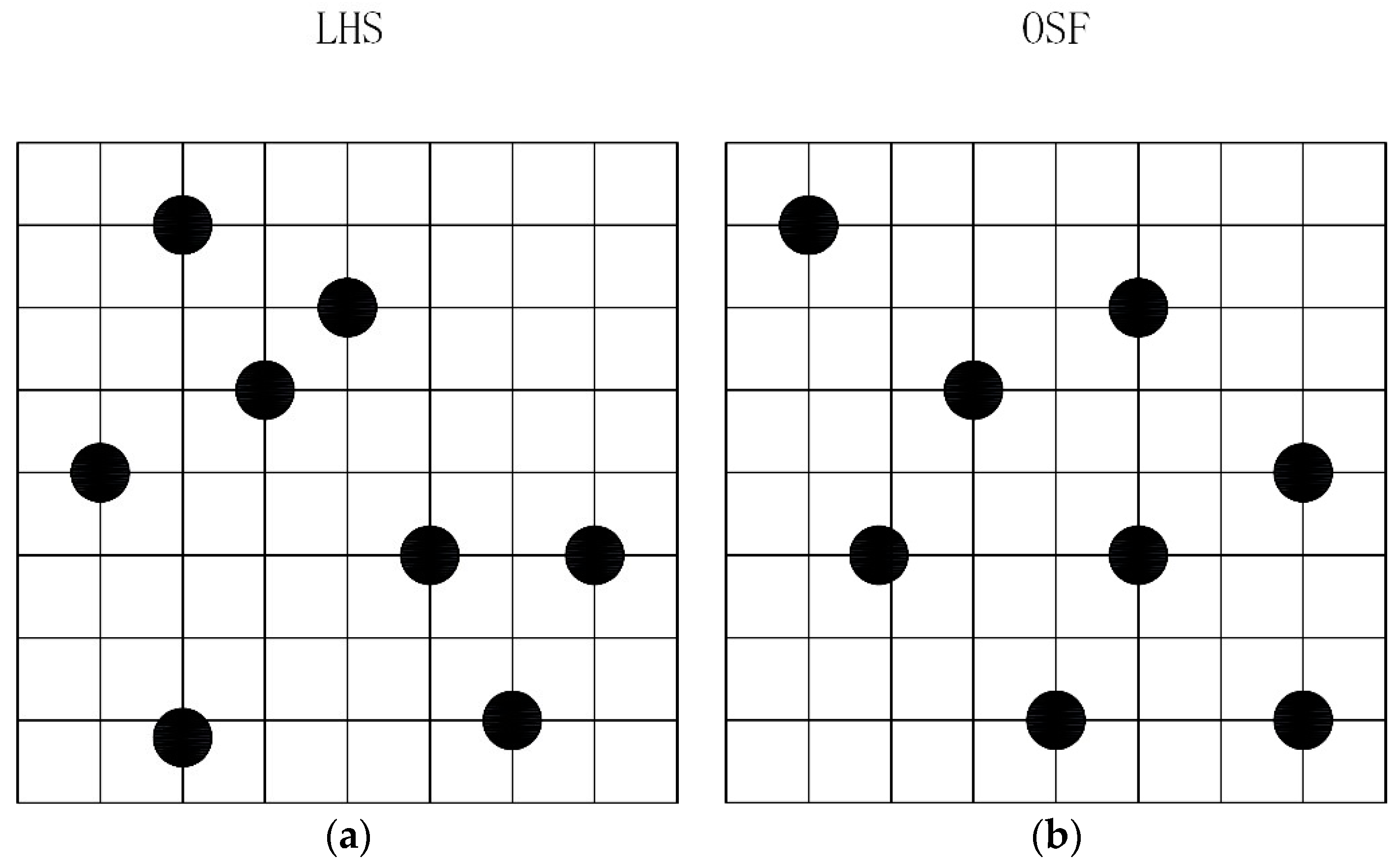
  • Given the space of four design variables, 80 uniformly distributed sample points are generated by the OSF method.
  • According to the sampling point, the CFD software Fluent is used to simulate the annular jet pump with different structural parameters. Through numerical simulation, the efficiency and head ratio of the annular jet pump are calculated.
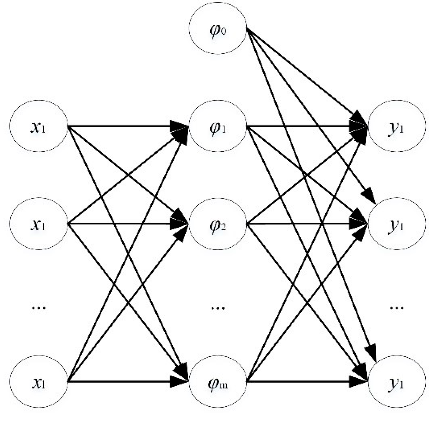
  • The neural network model is constructed via the RBF function. The structural parameters of the annular jet pump obtained at the sampling point in step 1 are the input variables, and the efficiency η and head ratio h of the jet pump obtained in step 2 are the output variables.
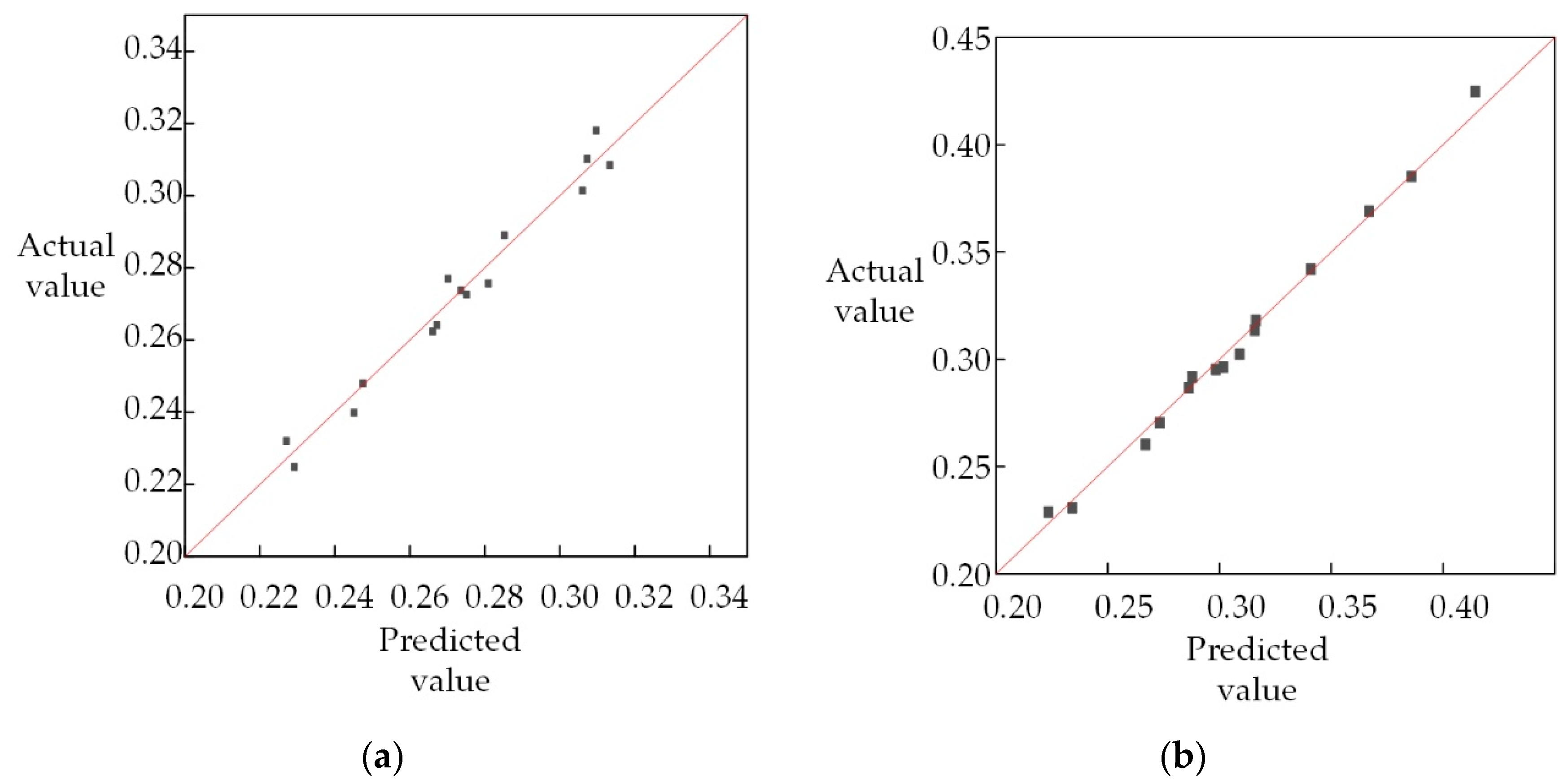
  • The RBF neural network model constructed in step 3 is verified, then the predicted values and simulated values are compared. If the error between the two sets of data is very small, move on to step 5; otherwise, return to step 3 and continue to update the RBF neural network model.
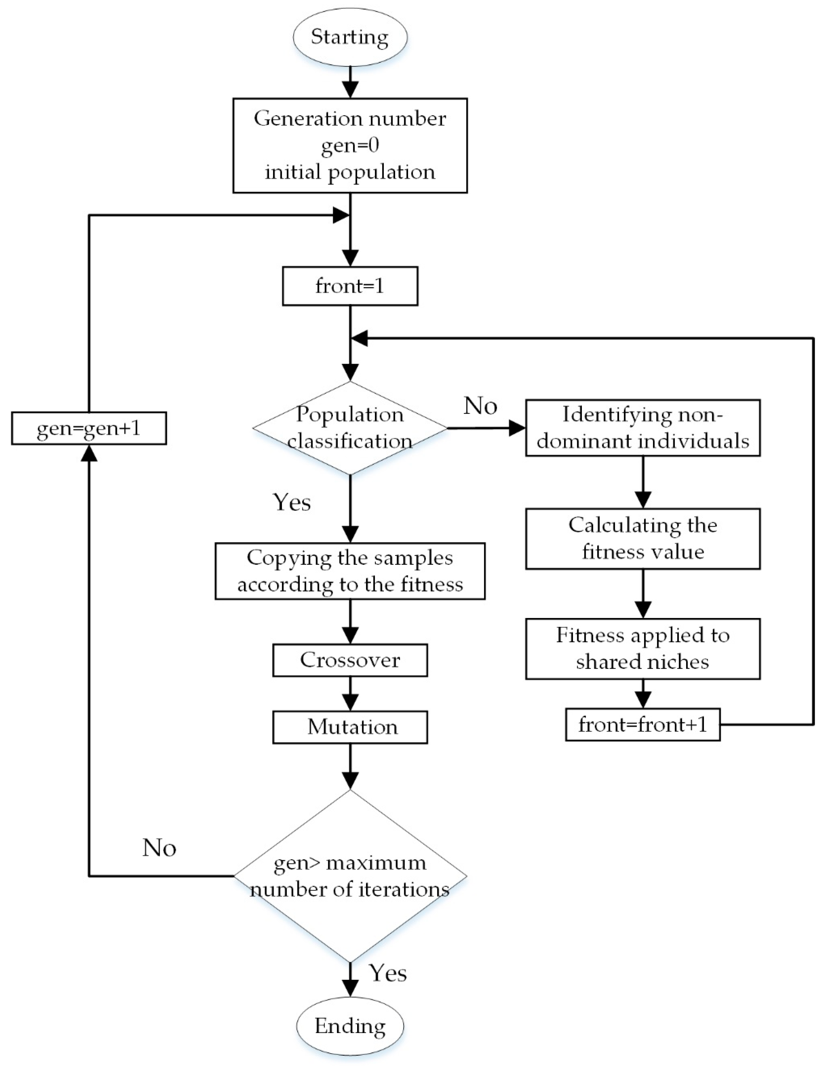
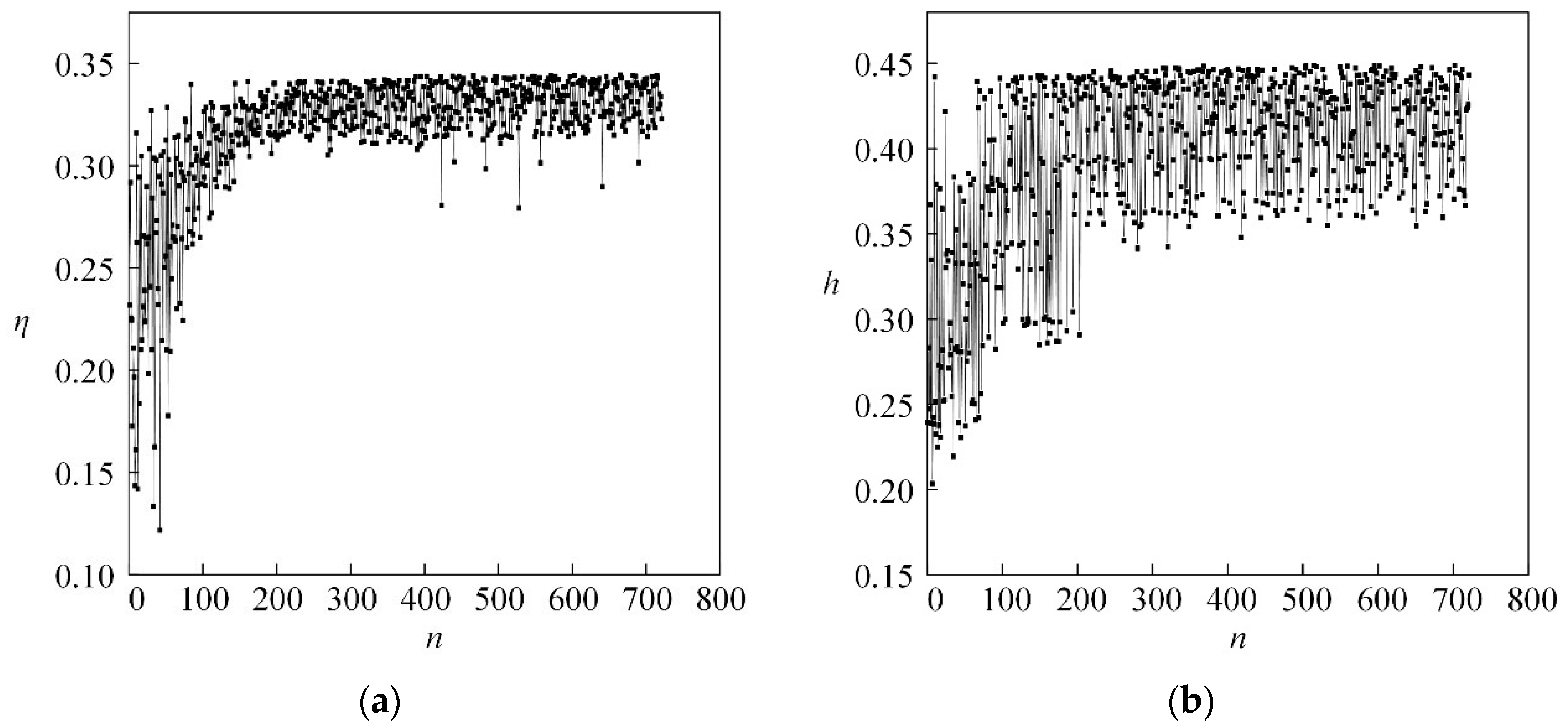
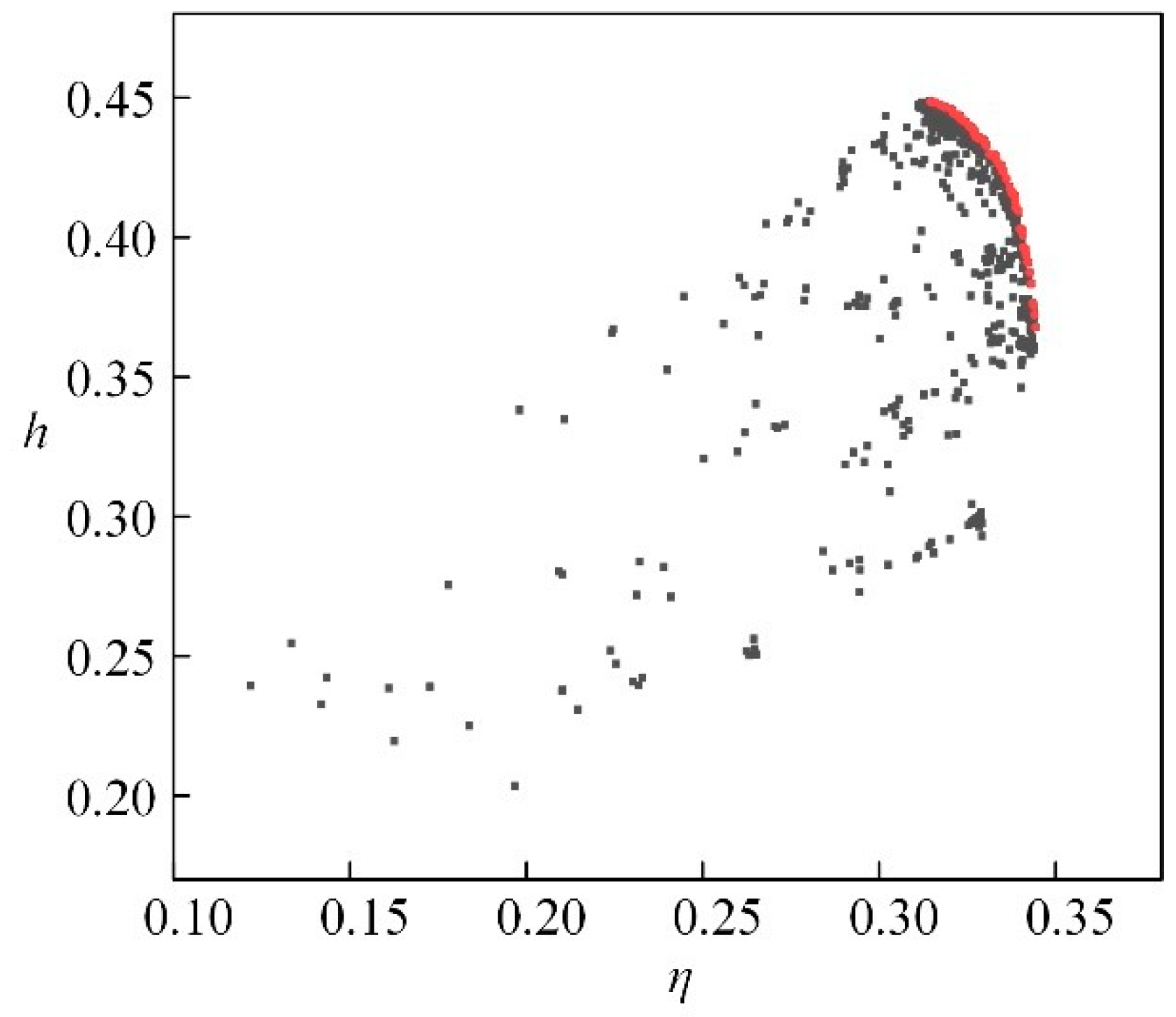
  • Based on the RBF neural network model, the NSGA-II optimization algorithm is used to get the optimal solution of the structural parameters of the annular jet pump.
  • According to the design parameters of the optimal solution, an optimization model is generated. The CFD simulation and optimization results of the optimization model are verified with each other.

4.2. DOE Method

The premise of determining optimization method reliability in this paper is to guarantee the reliability of the approximate model. DOE plays a decisive role in the quality of the approximate model.
Compared with traditional DOE methods, OSF is used in this paper to generate sample points in the design space. OSF is an improvement of the Latin hypercube sampling algorithm (LHS) that develops an efficient global optimal search algorithm, the enhanced stochastic evolutionary algorithm (ESE). The criteria for evaluating optimality is based on an entropy criterion, CL2 criterion, and a Φp criterion. The proposed algorithm is much more efficient compared with existing techniques in terms of the computation time, number of exchanges needed for generating new designs, and the achieved optimality criteria [35]. OSF improves the randomness of LHS and makes all sample points evenly distributed in the design space as much as possible to ensure good space-filling and uniformity. Therefore, OSF can better reflect the mapping relationship between factors and responses, which makes the fitting of factors and responses more accurate with the minimum sample points.
Figure 5a shows that the sampling points generated by LHS are randomly generated, and Figure 5b shows that the sampling points generated by OSF are evenly distributed. It can be seen that LHS lacks sample points in the upper right corner of the design space, which do not reflect the relationship between the factor and the response in this region. The use of OSF makes the sample points in the whole design space more uniform.

4.3. Approximate Model

The RBF model has a strong ability to approximate complex nonlinear functions. Because of its fast learning speed without a mathematical hypothesis or black box characteristics, the model has been extensively applied in function approximation, pattern recognition, financial systems, signal processing, power systems, expert systems, military systems, image processing and computer visions, medical control, and optimization [36,37]. In this paper, an RBF neural network is used to map the approximate function between the parameters of the jet pump and the objectives.
As illustrated in Figure 6, there are usually three layers in this neural network. On the left is the input layer with four neurons, which represent four design parameters. In the middle is the hidden layer with nine neurons; this contains a non-linear radial basis activation function. On the right is an output layer with two neurons that represent two objective parameters.
The radial basis function commonly applied in an RBF neural network is the Gaussian function, so the activation function of the RBF neural network can be described as
R ( x p c i ) = exp ( 1 2 σ 2 x p c i 2 )
where ‖xpci‖ is the Euclidean norm, σ is the variance of the Gaussian function and ci is the center of the Gaussian function.
According to the RBF neural network structure, the output of the RBF neural network is
y i = i = 1 h ω i j exp ( 1 2 σ 2 x p c i 2 ) j = 1 , , n
where x = ( x 1 p ,   x 2 p ,   ,   x n p ) is a p-th input sample, p = 1, 2, …, P; P is the total number of samples; ωij is the connection weight from hidden layer to output layer; i = 1, 2, …, h; h is the number of hidden layer nodes; and yi is the actual output of the j-th output node of the network corresponding to the input sample.

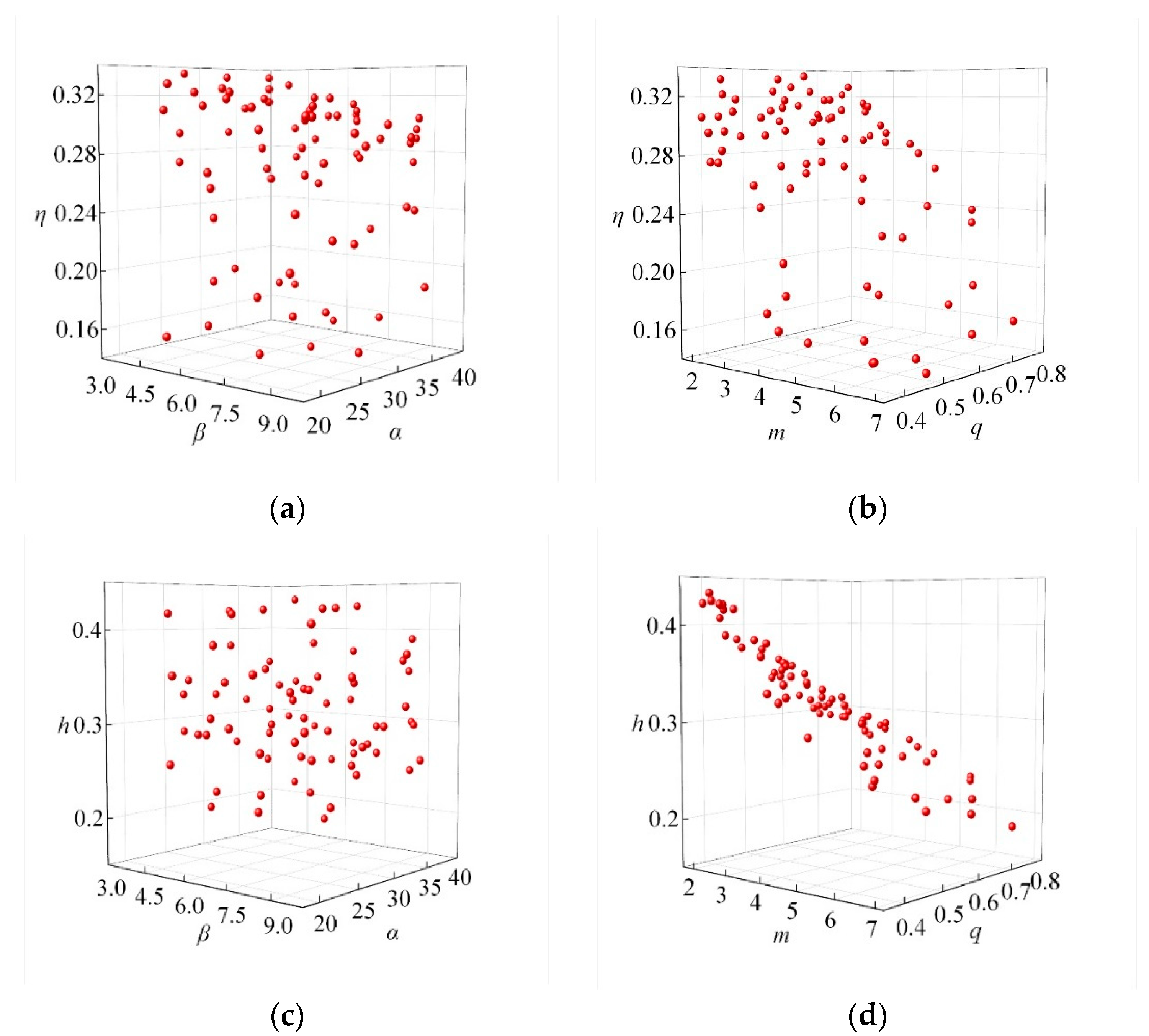
4.4. Establishment of Sample Database

Table A1 shows the design parameters of some sample points generated by OSF, as well as the corresponding jet pump efficiency and head ratio. The number of training samples should be at least 10 times the number of input variables [29]. Together with the number of test samples, a total of 80 samples are used. Figure 7 shows the three-dimensional distribution of 80 samples. It can be seen that the design parameters of sample points are evenly distributed in the parameter space. The best sample point of efficiency is No. 52 (q = 0.4354, m = 1.84, α = 27.74°, β = 4.76°), and the corresponding jet pump efficiency is 0.332. The best sample point for head ratio is No. 27 (q = 0.3728, m = 5.292, α = 34.98° and β = 5.292°), with a corresponding jet pump head ratio of 0.4329.

4.5. Multi Objective Optimization Algorithm

The jet pump objective functions are expressed as
{ M a x i m i z e η = f ( α , β , m , q ) M a x i m i z e h = f ( α , β , m , q )
which are subject to
{ 1.68 m 7.18 0.35 q 0.8 18 α 60 4 β 10
Traditional optimization algorithms contain a common weighting algorithm and constraint method. These methods convert the multi-objective function to a single-objective function by giving weight, then optimizing the single-objective function. This kind of algorithm is too ideal, and the optimization result is not good. Intelligent algorithms include common particle swarm optimizations, annealing algorithms, genetic algorithms and so on. These algorithms can reflect the essence of multi-objective optimization problems, and have been widely applied in recent years.
The NSGA-II [38] algorithm is used to optimize the jet pump in this paper. Compared with the simple GA (Genetic Algorithm), NSGA-II classifies the population according to the dominant relationship between individuals, giving higher-rated individuals a greater opportunity to pass on to the next generation. Compared with NSGA, NSGA-II has the following modifications: (1) A fast non-dominated sorting method to reduce the computational complexity of the algorithm. (2) A crowded comparison operator to replace the fitness sharing strategy that needs to specify the sharing radius. This is used as the criterion when comparing individuals at the same level after quick sorting, so that individuals of the Pareto solution set are extended to the whole Pareto domain and evenly distributed to maintain the diversity of the population. (3) An elite strategy to expand the sampling space. The parent population and its offspring are combined in the selection of the next generation’s population. This strategy helps retain the superior individuals from the parent generation in the subsequent generation. The best individuals will therefore not be lost, and the optimization level will be rapidly improved via the hierarchical storage of all the individuals in the population. This principle is shown in Figure 8.

5. Results and Discussion

5.1. Error Analysis of RBF Model

The design variables of 80 sample points generated by the OSF and the corresponding CFD simulation results are used as inputs and outputs to establish an RBF neural network approximate model. Specifically, the parameters α, β, m and q of the jet pump are input variables, and the corresponding efficiency η and head ratio h are the output variables. In this paper, Isight is used to train the RBF neural network model. Type of Basis Function is set as radial. The remaining parameters use default values. We use cross validation, with 65 sample points used as the training set and 15 sample points as the test set. Figure 9 shows the degree of fitting between the predicted value of the objective function and the simulated value of CFD. On the diagonal, the predicted value is equal to the CFD value. It can be seen that all the points distribute around the diagonal.
The average error of efficiency and head ratio is 4.8% and 1.7%, respectively. The maximum error of efficiency and head ratio are 8.6% and 6.1%, respectively. For further verification of the RBF model’s accuracy, a statistical measure of objective function, correlation coefficient R2, is introduced to estimate the approximate degree [39]. An R2 statistic that close to 1 indicates that a large proportion of the variability in the response is due to the regression. The correlation coefficient is defined as follows:
R 2 = 1 i = 1 n ( y i Y ) 2 i = 1 n ( y i y ¯ ) 2
After calculation, the R2 of efficiency and head ratio are 0.97033 and 0.99286, respectively, which meets the engineering requirement.

5.2. Optimization Results

In this paper, the crossover probability is set as 0.9, the number of generations is 20 and the initial population size is 36. After 721 genetic iterations, global optimization is carried out. Figure 10 shows the changing efficiency and head ratio trends for the annular jet pump, with an increase in iteration numbers during the optimization process. According to the trends observed during the optimization process for the two optimization objectives, it can be seen that the fluctuation range of efficiency has a small iteration number, while the fluctuation range of head ratio has a large iteration number.
Using the NSGA-II algorithm, the non-dominated solutions are obtained and the Pareto optimal frontier is shown after 721 iteration generations (Figure 11). This shows that the Pareto optimal solutions (red dots in the picture) are densely, continuously and smoothly distributed on a convex curve, indicating that NSGA-II has a strong ability to approximate Pareto solutions in the sample space.
It can be seen from the red Pareto optimal solutions in Figure 11 that the head ratio has a monotone decrease with increased efficiency in the Pareto optimal frontier, and there are some conflicts between the two objectives in this paper. The two objectives either cannot be compared, or may not be the optimal solutions for all objectives. The mapping primal points of these non-dominated solutions in the decision space, called Pareto solutions, are non-inferior.
Table 2 shows the comparison of structural parameters between the optimization scheme and the original scheme, and Table 3 shows a comparison of performance optimization objectives between the optimization scheme and the original scheme.
According to the two tables of parameters, it can be seen that, in terms of structure, the suction angle of the optimization model is increased, the diffusion angle is decreased and the flow ratio and area ratio are decreased, while in terms of performance, the head ratio of the optimization model is increased by 30.46%, and the efficiency is increased by 7%.

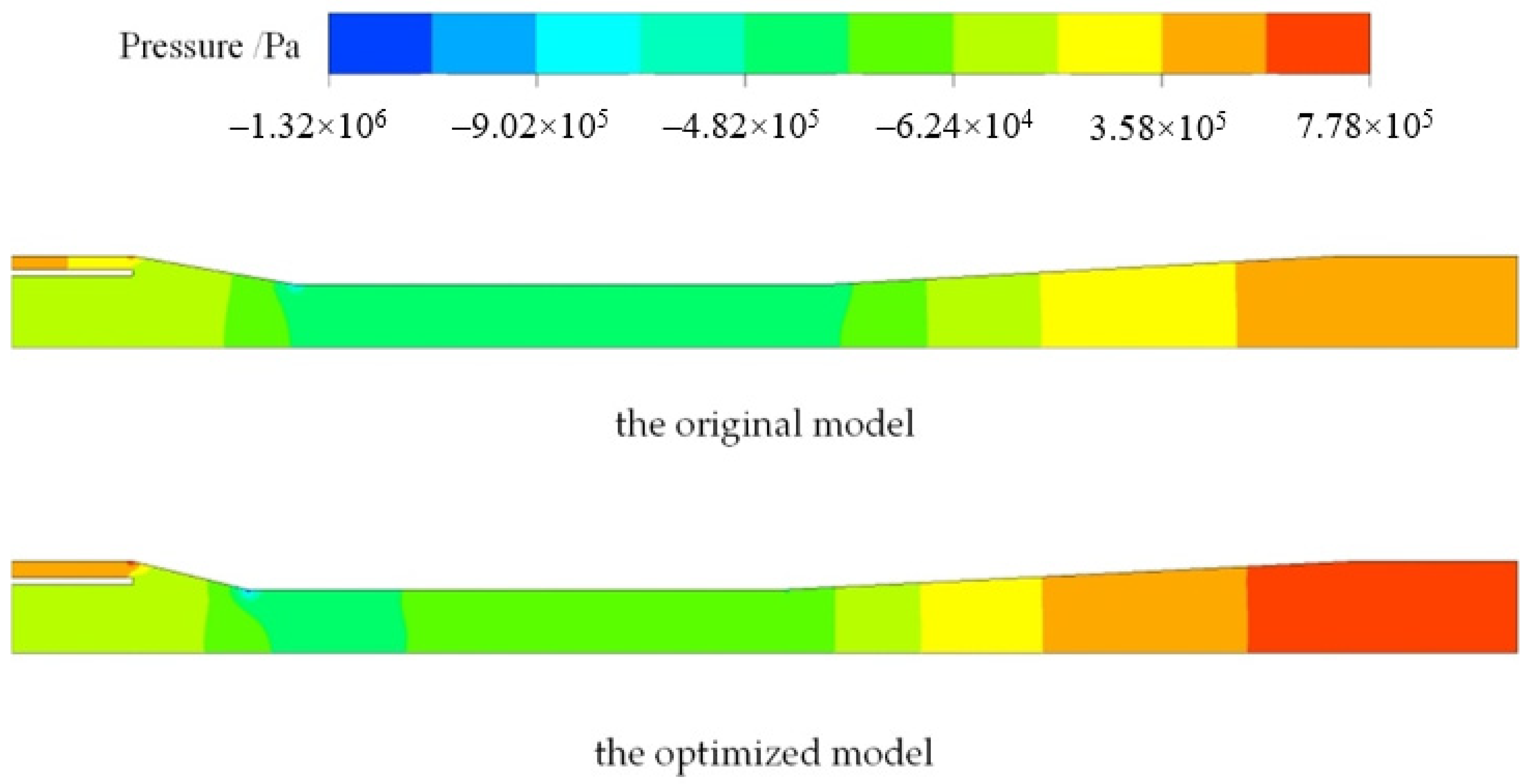
5.3. Analysis of Internal Flow Field Optimization of Jet Pump

Figure 12 shows a pressure field comparison between the original model and the optimized model. The pressure distribution in the suction chamber and throat of the optimized model is similar to that of the original model, but the high pressure region of the optimized model is widely distributed in the diffuser and outlet; that is, kinetic energy is converted into pressure energy earlier in the diffusion. In general, the inlet pressure is similar between the two models. The pressure gradient along the axial direction of the jet pump is more obvious and the outlet pressure is higher in the optimized model, which helps to improve the head ratio of the jet pump.

6. Conclusions

In this study, an annular jet pump optimization method was proposed based on a CFD simulation, RBF neural network model and NSGA-II optimization algorithm. The CFD simulation scheme was created and verified with experiment data, ensuring the reliability of the simulation results. The RBF neural network model was established by the OSF and verified by the CFD simulation results. In the end, the parameters of the annular jet pump were optimized using the NSGA-II algorithm.
According to the results of above, the following conclusions can be presented:
(1)
An RBF neural network approximation model was constructed to analyze the efficiency and head ratio of an annular jet pump. The determination coefficients R2 of the two objectives were greater than 0.97, and the accuracy of the model is reliable.
(2)
The NSGA-II algorithm was used to optimize the annular jet pump. In terms of structure, the suction angle increased, the diffusion angle decreased and the flow ratio and area ratio decreased compared with the original model, while in terms of performance, the head ratio increased by 30.46% and efficiency is increased by 7%.
(3)
The optimization method based on the RBF neural network model and the NSGA-II optimization algorithm was able obtain the optimal design parameter combination in the global design space of an annular jet pump, which can be applied to other kinds of pumps. However, due to the errors of the CFD and RBF models, this method needs the support of experimental data.

Author Contributions

Formal analysis, K.X. and G.W.; Methodology, K.X.; Writing—original draft preparation, K.X. and G.W.; Writing—review and editing, L.Z., L.W., F.Y., W.S. and X.C.; Validation, L.W. and X.W.; Supervision L.W.; Funding acquisition, G.W. and F.Y. All authors have read and agreed to the published version of the manuscript.

Funding

This research was funded by National Key Research and Development Project (Grant No. 2018YFF01012900), National Natural Science Foundation of China (Grant No. 51779059, 52001116, 52001089, 51779064), National Natural Science Foundation of Heilongjiang Province (Grant No. YQ2020E028, YQ2020E033), China Postdoctoral Science Foundation (Grant No. 2020M670889, 2018M630343), Fundamental Research Funds for the Central Universities (Grant No. 3072020CF0702, 3072020CFT0105, 3072020CFT0704), and the School Land Integration Development Project of Yantai (Grant No. 2019XDRHXMPT29).

Institutional Review Board Statement

Not applicable.

Informed Consent Statement

Not applicable.

Data Availability Statement

Not applicable.

Acknowledgments

The authors gratefully acknowledge the financial support from National Key Research and Development Project (Grant No. 2018YFF01012900), National Natural Science Foundation of China (Grant No. 51779059, 52001116, 52001089, 51779064), National Natural Science Foundation of Heilongjiang Province (Grant No. YQ2020E028, YQ2020E033), China Postdoctoral Science Foundation (Grant No. 2020M670889, 2018M630343), Fundamental Research Funds for the Central Universities (Grant No. 3072020CF0702, 3072020CFT0105, 3072020CFT0704), and the School Land Integration Development Project of Yantai (Grant No. 2019XDRHXMPT29).

Conflicts of Interest

The authors declare no conflict of interest.

Appendix A

Table A1. Design parameters and efficiency of DOE sample points.
qmα(°)β(°)
0.58354.25620.229.164
0.72591.78930.547.646
0.5382.45418.848.178
0.40134.07820.58.936
0.38994.87636.18.026
0.64623.01931.924.228
0.42971.95921.346.734
0.38424.34925.244.988
0.36712.64926.088.556
0.36142.49134.447.722
0.7432.18536.664.608
0.70893.68824.124.076
0.68611.88337.59.012
0.46392.82429.984.152
0.6692.872408.406
0.62916.16335.545.14
0.78865.38323.025.67
0.67471.72330.825.444
0.73162.91920.785.974
0.354.54727.187.266
0.69181.98519.687.114
0.6123.99528.586.126
0.75442.52929.145.898
0.76583.83527.467.494
0.78293.91536.947.038
0.63481.81238.326.582
0.37282.2834.985.292
0.55512.15533.047.95
0.68046.34721.97.494
0.65762.01229.429.772
0.60636.95323.35.368
0.50386.73731.086.886
0.77724.44731.365.216
0.47533.41933.66.506
0.59492.96833.329.62
0.57222.31318.285.518
0.76012.69132.768.784
0.50953.48226.647.798
0.44685.99228.589.088
0.48673.01939.168.482
0.54942.38228.026.05
0.46392.06731.6410
0.77155.52423.849.392
0.6122.24824.964
0.41273.29632.489.696
0.74871.93322.745.064
0.4073.1819.46.658
0.58353.7618.566.81
0.53235.24936.389.468
0.52092.73524.689.848
0.43541.83527.744.76
0.4811.70233.886.278
0.79432.18537.226.962
0.70327.17832.27.114
0.62344.99428.868.86
0.60064.65237.787.342
0.54373.54822.184.684
0.35574.16634.444.836
0.45825.82938.885.746
0.73733.23719.128.33
0.69753.12525.89.924
0.57781.68123.565.822
0.39561.76729.78.102
0.42411.90821.629.316
0.56651.74525.528.254
0.52663.29638.064.532
0.65192.56826.367.874
0.37852.60827.186.202
0.49816.53622.467.418
0.51525.11730.264.304
0.56082.0434.74.38
0.72034.7635.829.24
0.44111.85938.68.708
0.66332.09619.949.544
0.82.12424.48.632
0.71463.61639.444.912
0.45255.675185.518
0.64052.77935.266.43
0.49242.34739.726.354
0.41842.41721.064.456

References

  1. Yapıcı, R.; Aldas, K. Optimization of water jet pumps using numerical simulation. Proc. Inst. Mech. Eng. Part A J. Power Energy 2013, 227, 438–449. [Google Scholar] [CrossRef]
  2. Meakhail, T.; Teaima, I. Experimental and numerical studies of the effect of area ratio and driving pressure on the performance of water and slurry jet pumps. Proc. Inst. Mech. Eng. Part C J. Mech. Eng. Sci. 2012, 226, 2250–2266. [Google Scholar] [CrossRef]
  3. Long, X.; Xu, M.; Wang, J.; Zou, J.; Bin, J. An experimental study of cavitation damage on tissue of Carassius auratus in a jet fish pump. Ocean Eng. 2019, 174, 43–50. [Google Scholar] [CrossRef]
  4. Shimizu, Y.; Nakamura, S.; Kuzuhara, S. Studies of the Configuration and Performance of Annular Type Jet Pumps. J. Fluids Eng. 1987, 3, 205–212. [Google Scholar] [CrossRef]
  5. Kwon, O.B.; Kim, M.K.; Kwon, H.C.; Bae, D.S. Two-dimensional Numerical Simulations on the Performance of an Annular Jet Pump. J. Vis. 2002, 5, 21–28. [Google Scholar] [CrossRef]
  6. Deng, H.; Liu, X.; Ma, W. Flow Field Analysis for the Diffuser Outlet of Jet Pump Used in the Drain Sand of Petroleum Well. J. Jilin Univ. 2010, 40, 689–693. [Google Scholar] [CrossRef]
  7. Yang, X.; Long, X.; Yao, X. Numerical investigation on the mixing process in a steam ejector with different nozzle structures. Int. J. Therm. Sci. 2012, 56, 95–106. [Google Scholar] [CrossRef]
  8. Lyu, Q.; Xiao, Z.; Zeng, Q.; Xiao, L.; Long, X. Implementation of design of experiment for structural optimization of annular jet pumps. J. Mech. Sci. Technol. 2016, 30, 585–592. [Google Scholar] [CrossRef]
  9. Deng, X.; Dong, J.; Wang, Z.; Tu, J. Numerical analysis of an annular water–air jet pump with self-induced oscillation mixing chamber. J. Comput. Multiph. Flows 2017, 9, 47–53. [Google Scholar] [CrossRef]
  10. Wang, X.; Chen, Y.; Li, M.; Xu, Y.; Wang, B.; Dang, X. Numerical Study on the Working Performance of a Streamlined Annular Jet Pump. Energies 2020, 13, 4411. [Google Scholar] [CrossRef]
  11. Gao, G.; Xing, Y.; Wang, Y. Effect of Nozzle Throat Geometry on Flow Field in Liquid Gas Jet Pump: A Simulation Study. Chin. J. Vac. Sci. Technol. 2020, 40, 174–179. [Google Scholar] [CrossRef]
  12. Xu, M.; Yang, X.; Long, X.; Lyu, Q. Large eddy simulation of turbulent flow structure and characteristics in an annular jet pump. J. Hydrodyn. 2017, 2, 702–715. [Google Scholar] [CrossRef]
  13. Zou, C.H.; Li, H.; Tang, P.; Xu, D.H. Effect of structural forms on the performance of a jet pump for a deep well jet pump. In Proceedings of the Computational Methods and Experimental Measurements XVII, International Conference on Computational Methods and Experimental Measurements 17th, Opatija, Croatia, 5 May 2015. [Google Scholar] [CrossRef] [Green Version]
  14. Elger, D.; Taylor, S.; Liou, C. Recirculation in an Annular-Type Jet Pump. J. Fluids Eng. 1994, 116, 735–740. [Google Scholar] [CrossRef]
  15. Keeney, R.; Raifa, H. Decisions with Multiple Objectives: Preferences and Value Tradeoffs. Health Serv. Res. 1978, 13, 1093–1094. [Google Scholar] [CrossRef]
  16. Marler, R.; Arora, J. Survey of multi-objective optimization methods for engineering. Struct. Multidiscip. Optim. 2004, 26, 369–395. [Google Scholar] [CrossRef]
  17. Chen, W.; Wiecek, M.; Zhang, J. Quality utility: A compromise programming approach to robust design. ASME J. Mech. Des. 1999, 121, 179–187. [Google Scholar] [CrossRef] [Green Version]
  18. Luh, G.; Chueh, C.; Liu, W. MOIA: Multi-objective immune algorithm. Eng. Optim. 2003, 35, 143–164. [Google Scholar] [CrossRef]
  19. Deb, K.; Jain, S. Multi-Speed Gearbox Design Using Multi-Objective Evolutionary Algorithms. ASME J. Mech. Des. 2003, 125, 609–619. [Google Scholar] [CrossRef] [Green Version]
  20. Saitou, K.; Cetin, O. Decomposition-Based Assembly Synthesis for Structural Modularity. ASME J. Mech. Des. 2004, 126, 234–243. [Google Scholar] [CrossRef]
  21. Ma, X.; Li, Y.; Yan, L. Comparsion review of traditional multi-objective optimization methods and multi-objective genetic algorithm. Electr. Drive Autom. 2010, 3, 48–50. [Google Scholar] [CrossRef]
  22. Barthelemy, J.; Haftka, R. Approximation concepts for optimum structural design—A review. Struct. Multidiscip. Optim. 1993, 5, 129–144. [Google Scholar] [CrossRef]
  23. Alexandras, A. Stochastic subset optimization incorporating moving least squares response surface methodologies for stochastic sampling. Adv. Eng. Softw. 2012, 44, 3–14. [Google Scholar] [CrossRef]
  24. Gholap, A.; Khan, J. Design and multi-objective optimization of heat exchangers for refrigerators. Appl. Energy 2007, 84, 1226–1239. [Google Scholar] [CrossRef]
  25. Verstraete, T.; Alsalihi, Z.; Braembussche, R. Multidisciplinary Optimization of a Radial Compressor for Microgas Turbine Applications. J. Turbomach. 2010, 132, 031004. [Google Scholar] [CrossRef]
  26. Naseri, M.; Othman, F. Determination of the length of hydraulic jumps using artificial neural networks. Adv. Eng. Softw. 2012, 48, 27–31. [Google Scholar] [CrossRef]
  27. Frédéric, M.; Luis, A.; Ichiro, H. Efficient preconditioning for image reconstruction with radial basis functions. Adv. Eng. Softw. 2007, 38, 320–327. [Google Scholar] [CrossRef]
  28. Sun, H.; Schafer, M. Reduced order model assisted evolutionary algorithms for multi-objective flow design optimization. Eng. Optim. 2011, 43, 97–114. [Google Scholar] [CrossRef]
  29. Zhang, Y.; Hu, S.; Wu, J. Multi-objective optimization of double suction centrifugal pump using Kriging metamodels. Adv. Eng. Softw. 2014, 74, 16–26. [Google Scholar] [CrossRef]
  30. Safikhani, H.; Khalkhali, A.; Farajpoor, M. Pareto Based Multi-Objective Optimization of Centrifugal Pumps Using CFD, Neural Networks and Genetic Algorithms. Eng. Appl. Comp. Fluid. Mech. 2011, 5, 37–48. [Google Scholar] [CrossRef] [Green Version]
  31. Wang, C.; Hu, B.; Feng, Y.; Liu, K. Multi-objective optimization of double vane pump based on radial basis neural network and particle swarm. Trans. Chin. Soc. Agric. Eng. 2019, 35, 25–32. [Google Scholar] [CrossRef]
  32. Zhao, A.; Lai, Z.; Wu, P. Multi-objective optimization of a low specific speed centrifugal pump using an evolutionary algorithm. Eng. Optim. 2016, 48, 1251–1274. [Google Scholar] [CrossRef]
  33. Sheha, A.A.A.; Nasr, M.; Hosien, M.A.; Wahba, E.M. Computational and Experimental Study on the Water-Jet Pump Performance. J. Appl. Fluid Mech. 2018, 11, 1013–1020. [Google Scholar] [CrossRef]
  34. Shih, T.; Liou, W.; Shabbir, A.; Yang, Z.; Zhu, J. A new k-ε eddy viscosity model for high reynolds number turbulent flows. Comput. Fluids 1995, 24, 227–238. [Google Scholar] [CrossRef]
  35. Jin, R.; Chen, W.; Sudjianto, A. An efficient algorithm for constructing optimal design of computer experiments. J. Stat. Plan. Infer. 2005, 134, 268–287. [Google Scholar] [CrossRef]
  36. Amini, A.; Taki, M.; Rohani, A. Applied improved RBF neural network model for predicting the broiler output energies. Appl. Soft Comput. 2020, 87, 106006. [Google Scholar] [CrossRef]
  37. Wang, Y.; Chen, Z.; Zu, H.; Zhang, X. An Optimized RBF Neural Network Based on Beetle Antennae Search Algorithm for Modeling the Static Friction in a Robotic Manipulator Joint. Math. Probl. Eng. 2020, 2020, 1024–1034. [Google Scholar] [CrossRef] [Green Version]
  38. Deb, K.; Amrit, P.; Sameer, A.; Meyarivan, T. A fast and elitist multiobjective genetic algorithm: NSGA-II. IEEE Trans. Evol. Comput. 2002, 6, 182–197. [Google Scholar] [CrossRef] [Green Version]
  39. Kajero, O.; Thorpe, R.; Yao, Y.; Hill, W.; David, S.; Chen, T. Meta-model-based calibration and sensitivity studies of computational fluid dynamics simulation of jet pumps. Chem. Eng. Technol. 2017, 40, 1674–1684. [Google Scholar] [CrossRef]
Figure 1. Structural schematic drawing of annular jet pump.
Jmse 09 00236 g001
Figure 2. The computational domain.
Jmse 09 00236 g002
Figure 3. Experiment and simulation data. (a) Efficiency; (b) head ratio.
Jmse 09 00236 g003
Figure 4. The optimization flow.
Jmse 09 00236 g004
Figure 5. Design of experiments (DOE) method. (a) Latin hypercube sampling algorithm (LHS); (b) optimum space filling algorithm (OSF).
Jmse 09 00236 g005
Figure 6. RBF model structure.
Jmse 09 00236 g006
Figure 7. Performance of different sampling points. (a) η corresponding to α and β; (b) η corresponding to m and q; (c) h corresponding to α and β; (d) h corresponding to m and q.
Jmse 09 00236 g007
Figure 8. NSGA-II algorithm schematic.
Jmse 09 00236 g008
Figure 9. Error analysis. (a) Efficiency; (b) head ratio.
Jmse 09 00236 g009
Figure 10. Trends of pump efficiency and head ratio during the searching process. (a) Efficiency; (b) head ratio.
Jmse 09 00236 g010
Figure 11. Optimization results of the NSGA-II algorithm.
Jmse 09 00236 g011
Figure 12. Pressure distribution of annular jet pump.
Jmse 09 00236 g012
Table 1. The results with different numbers of elements.
Number of Elementshe
coarse0.57930.0924
medium0.57980.0926
fine0.58260.0936
Table 2. Comparison of design parameters between original scheme and optimized scheme.
α(°)β(°)mq
Original scheme185.82.270.5789
Optimized scheme25.025.17681.68230.3702
Table 3. Comparison of optimization objectives between the original scheme and optimized scheme.
ηh
Original scheme0.33250.3648
Optimized scheme0.35580.4758
Publisher’s Note: MDPI stays neutral with regard to jurisdictional claims in published maps and institutional affiliations.

