
The Effect of Wave-Induced Current and Coastal Structure on Sediment Transport at the Zengwen River Mouth †

Abstract
:1. Introduction
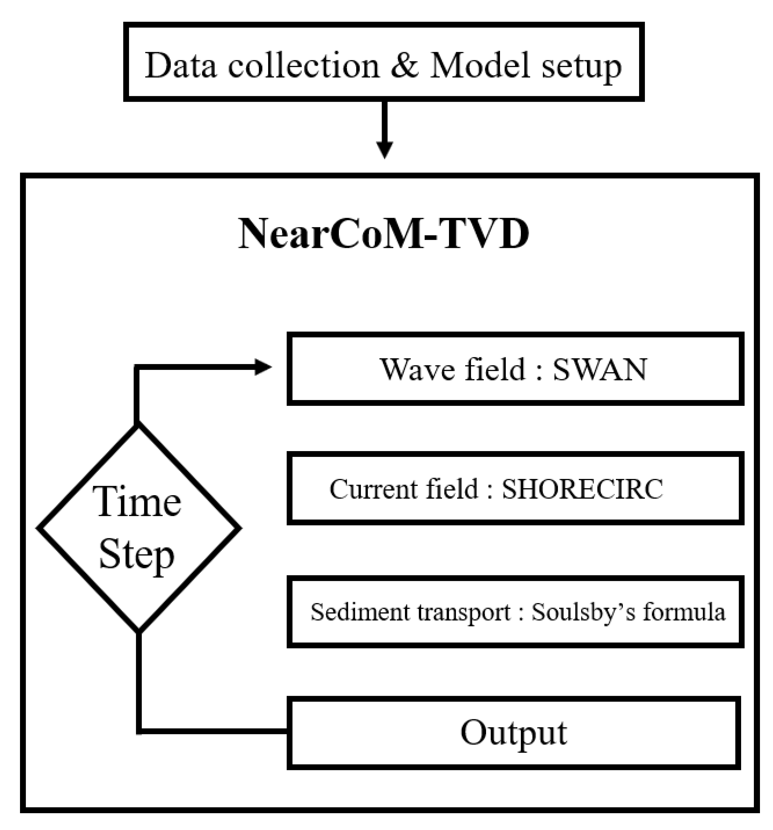
2. Numerical Model
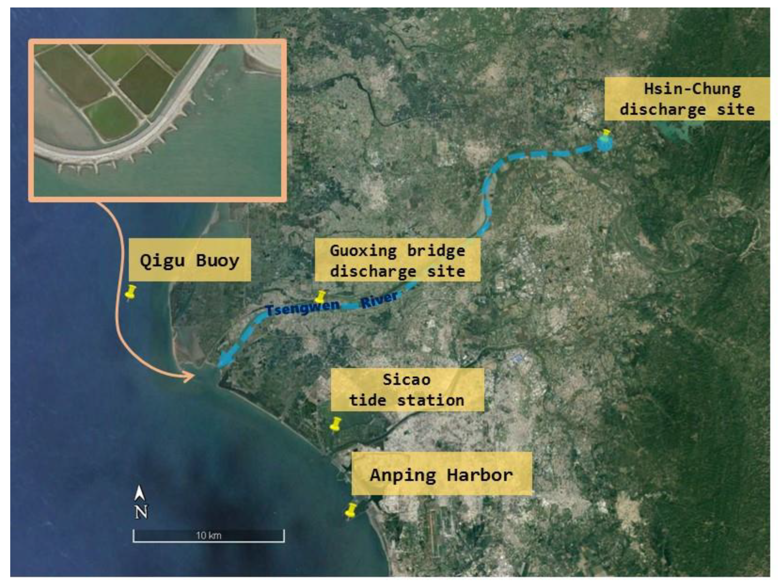
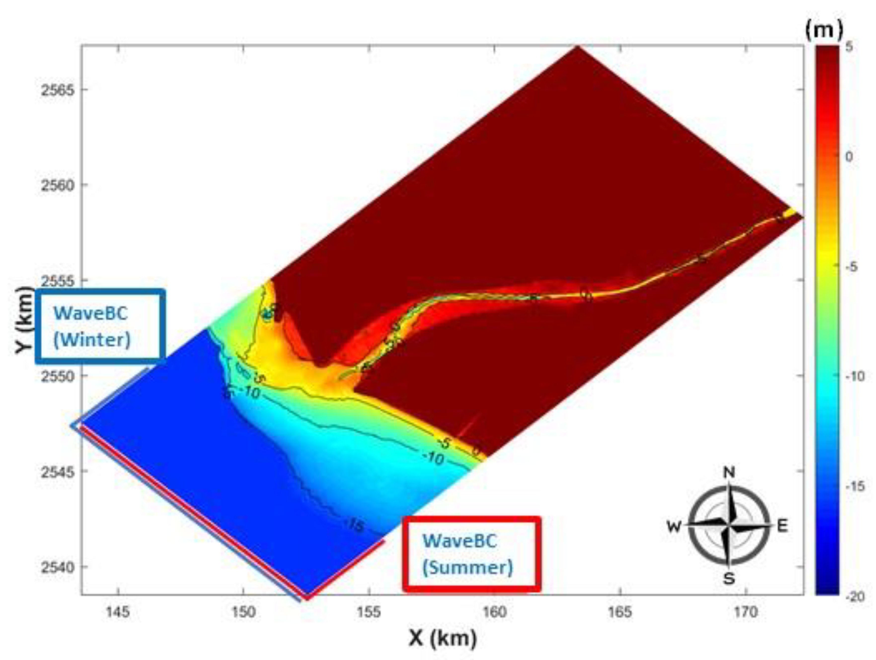
3. Model Configuration
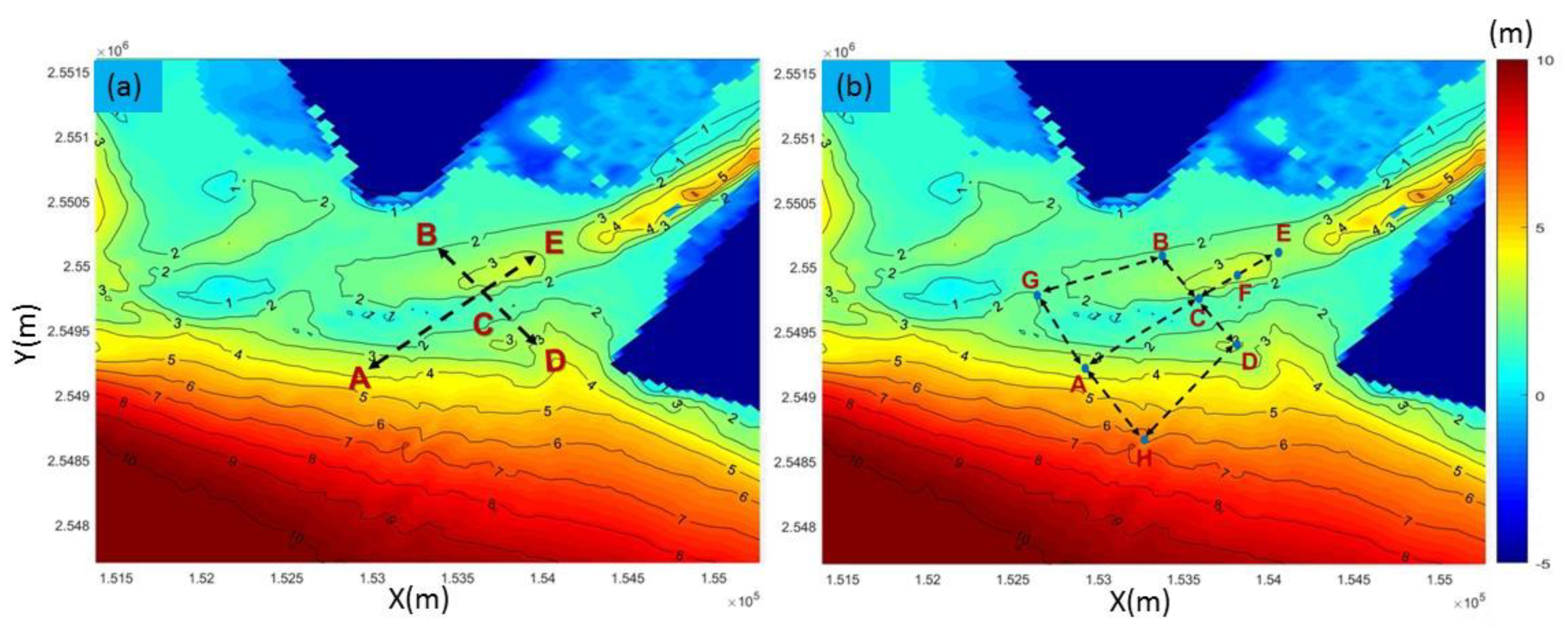
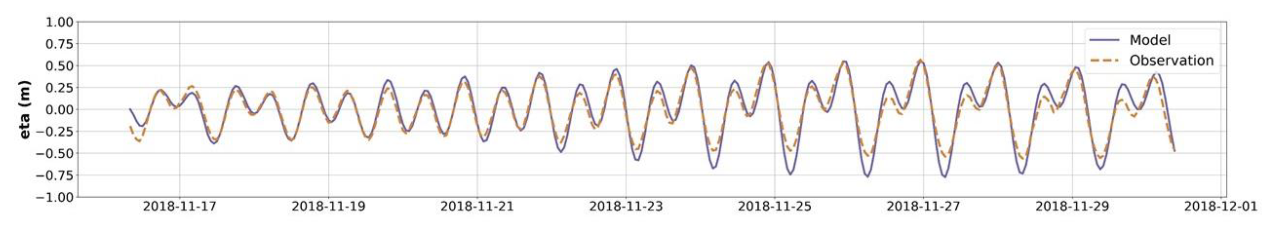
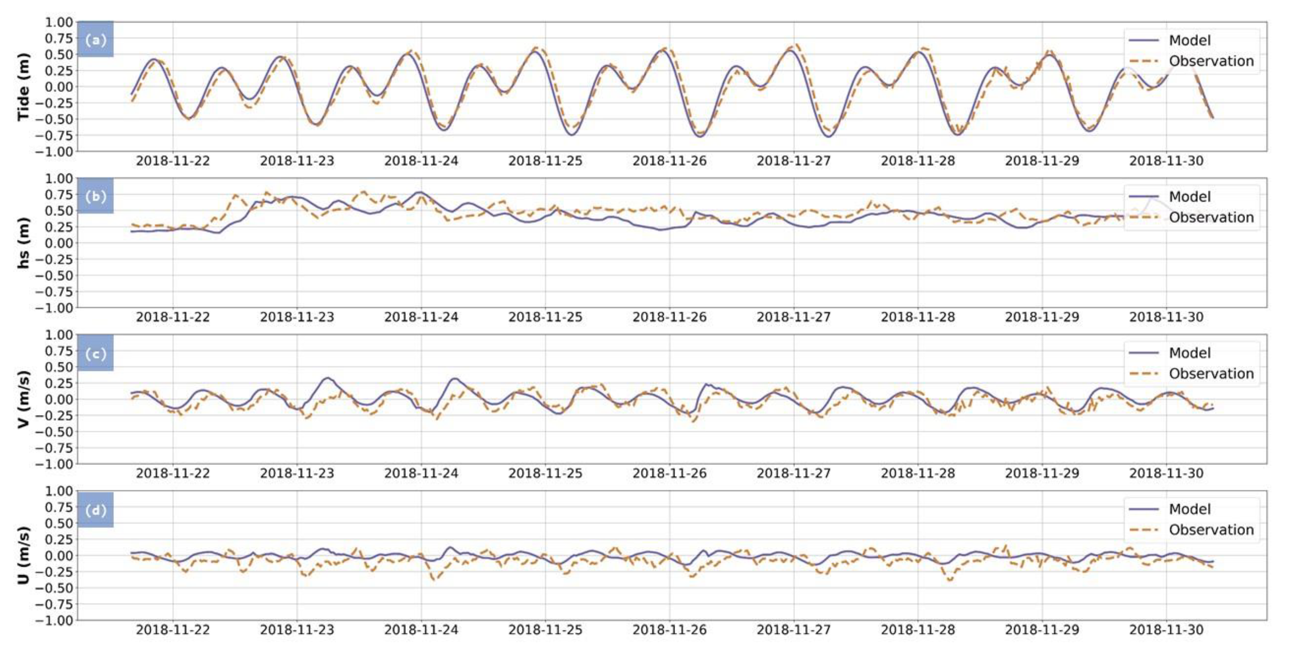
4. Model Validation and Statistic Error Analysis
5. Model Result and Discussion
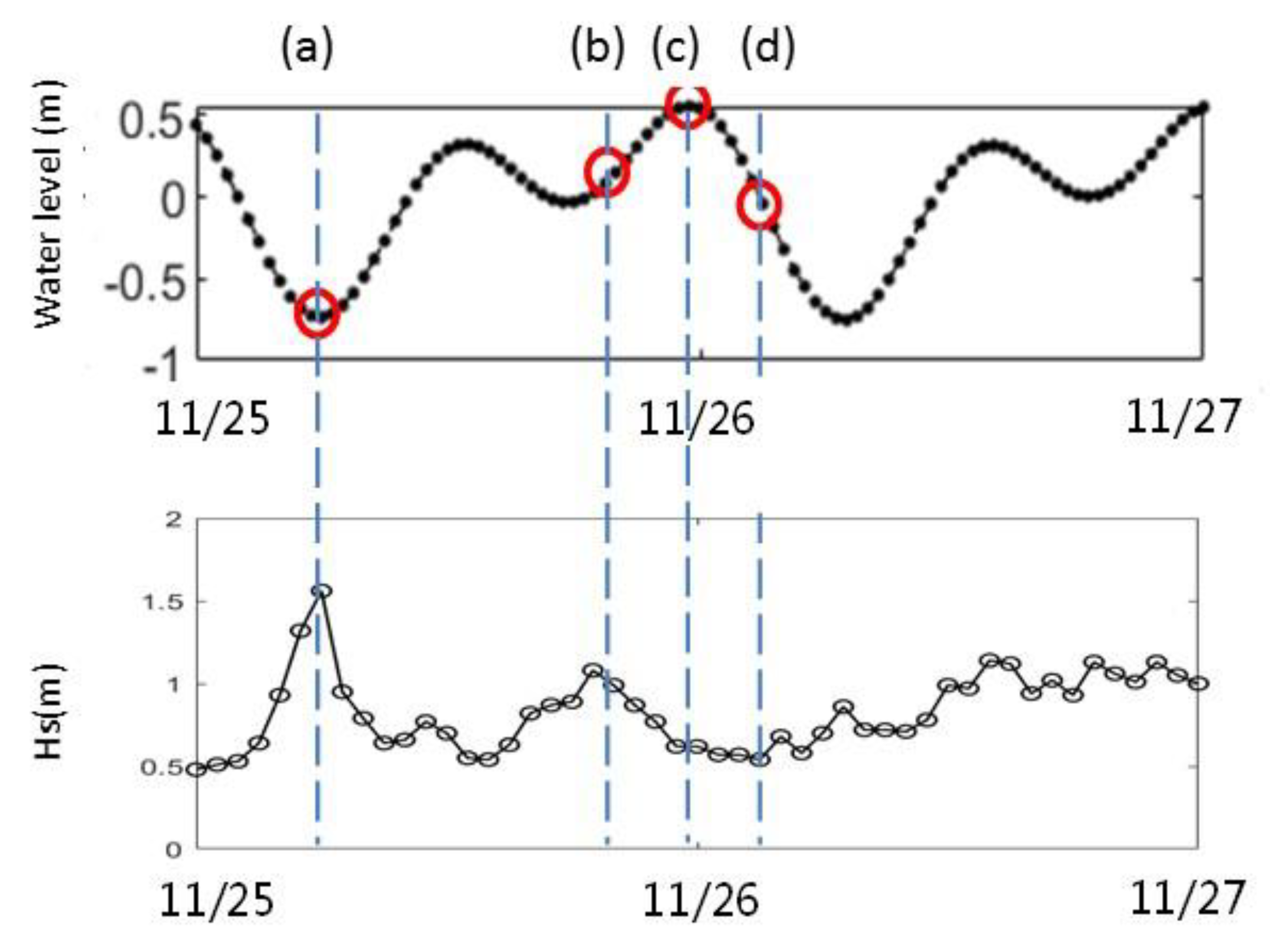
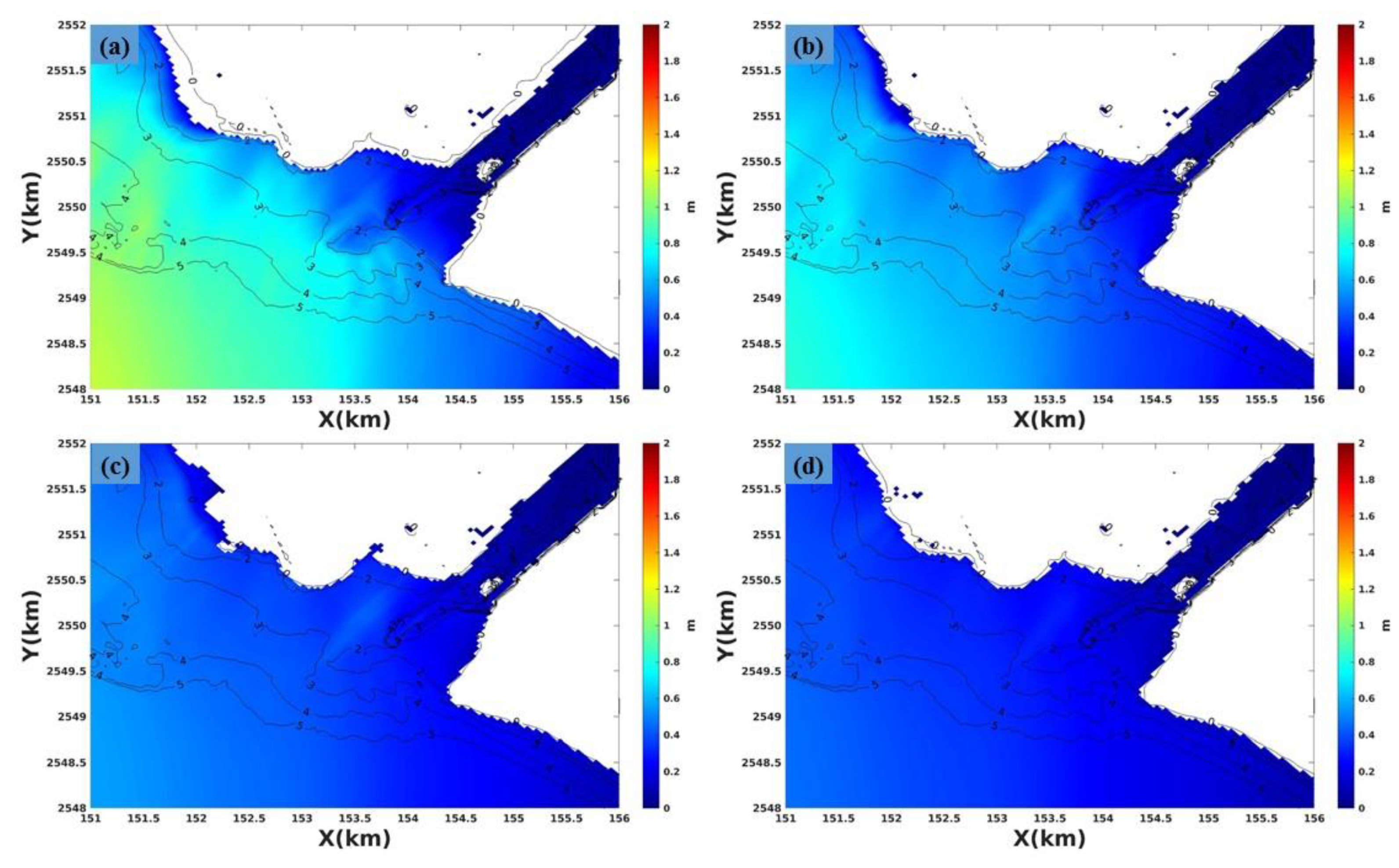
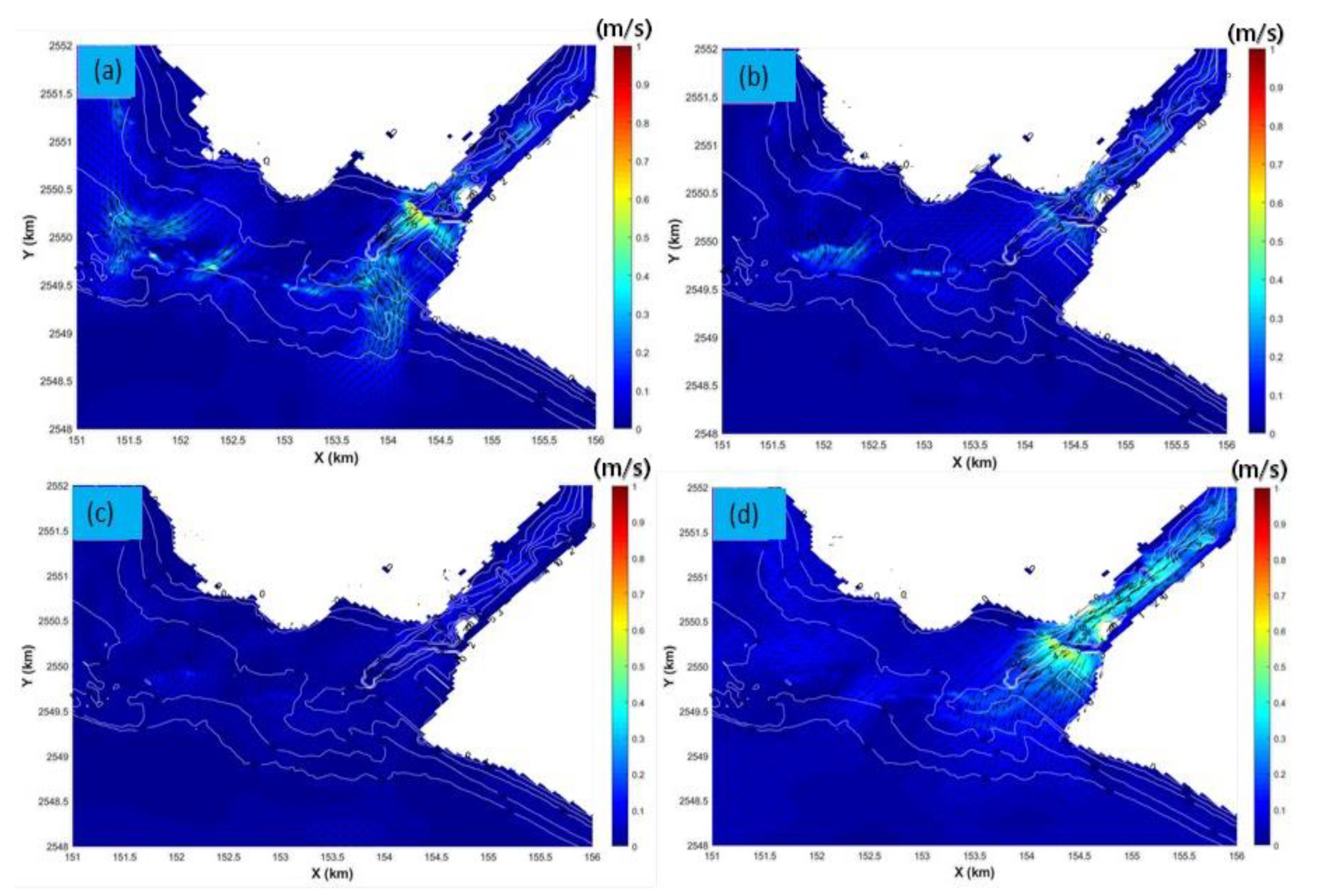
5.1. Wave and Flow Field under Different Tidal Hours
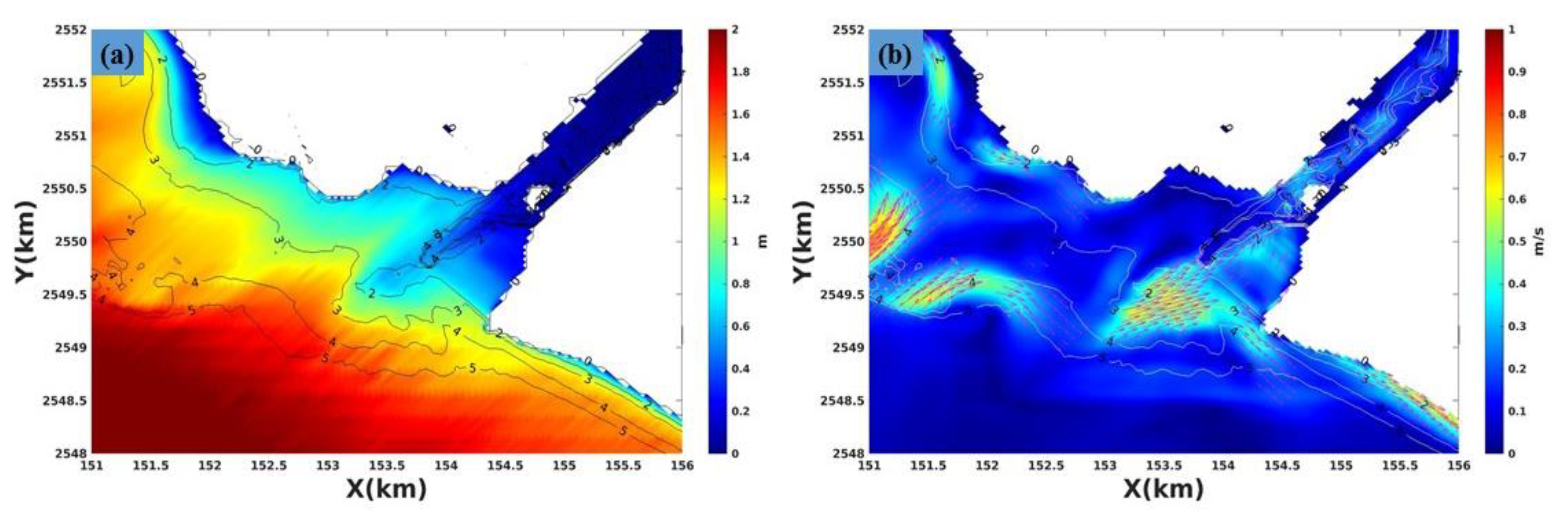
5.2. The Seasonal Variations of Wave and Flow Field
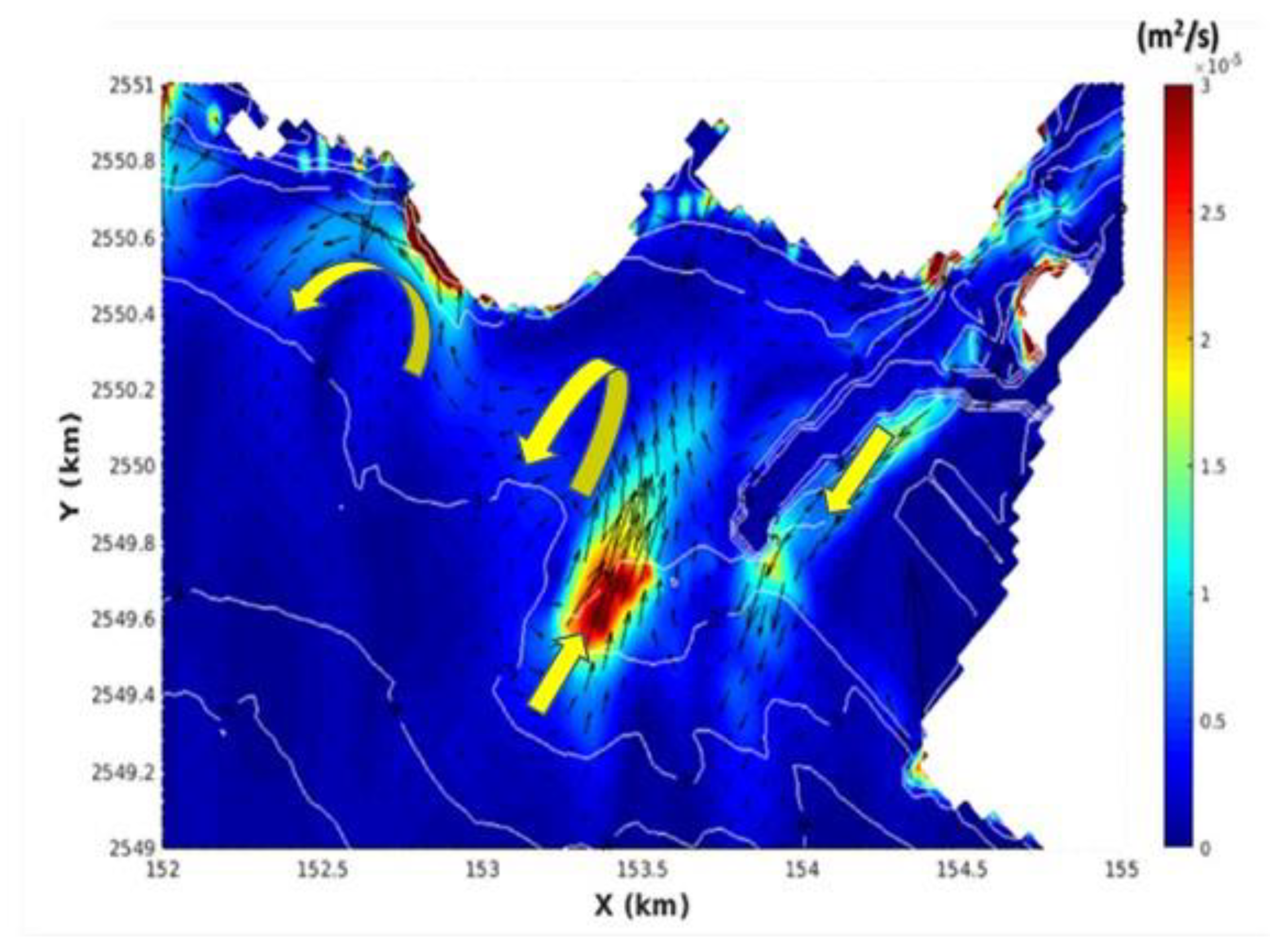
5.3. The Residual Sediment Transport and Morphological Evolution
6. Conclusions
Author Contributions
Funding
Acknowledgments
Conflicts of Interest
References
- Elias, E.; Cleveringa, J.; Buijsman, M.; Roelvink, J.; Stive, M. Field and model data analysis of sand transport patterns in Texel Tidal inlet (the Netherlands). Coast. Eng. 2006, 53, 505–529. [Google Scholar] [CrossRef]
- Malhadas, M.S.; Leitão, P.C.; Silva, A.; Neves, R. Effect of coastal waves on sea level in Óbidos Lagoon, Portugal. Cont. Shelf Res. 2009, 29, 1240–1250. [Google Scholar] [CrossRef]
- Bertin, X.; Fortunato, A.B.; Oliveira, A. A modeling-based analysis of processes driving wave-dominated inlets. Cont. Shelf Res. 2009, 29, 819–834. [Google Scholar] [CrossRef]
- Keshtpoor, M.; Puleo, J.A.; Shi, F.; DiCosmo, N.R. Numerical Simulation of Nearshore Hydrodynamics and Sediment Transport Downdrift of a Tidal Inlet. J. Waterw. Port Coastal Ocean Eng. 2015, 141, 04014035. [Google Scholar] [CrossRef]
- Milliman, J.; Lin, S.; Kao, S.; Liu, J.; Liu, C.; Chiu, J.; Lin, Y. Short-term changes in seafloor character due to flood-derived hyperpycnal discharge: Typhoon Mindulle, Taiwan, July 2004. Geology 2007, 35, 779. [Google Scholar] [CrossRef] [Green Version]
- Chien, H.; Chiang, W.-S.; Kao, S.-J.; Liu, J.; Liu, K.-K.; Liu, P. Sediment Dynamics Observed in the Jhoushuei River and Adjacent Coastal Zone in Taiwan Strait. Oceanography 2011, 24, 122–131. [Google Scholar] [CrossRef] [Green Version]
- Olabarrieta, M.; Geyer, W.R.; Kumar, N. The role of morphology and wave-current interaction at tidal inlets: An idealized modeling analysis. J. Geophys. Res. Ocean. 2014, 119, 8818–8837. [Google Scholar] [CrossRef] [Green Version]
- Chen, J.-L.; Ralston, D.K.; Geyer, W.R.; Sommerfield, C.K.; Chant, R.J. Wave Generation, Dissipation, and Disequilibrium in an Embayment With Complex Bathymetry. J. Geophys. Res. Ocean. 2018, 123, 7856–7876. [Google Scholar] [CrossRef]
- Rogowski, P.; Terrill, E.; Chen, J. Observations of the frontal region of a buoyant river plume using an autonomous underwater vehicle. J. Geophys. Res. Ocean. 2014, 119, 7549–7567. [Google Scholar] [CrossRef]
- Chen, J.L.; Hsu, T.; Shi, F.; Raubenheimer, B.; Elgar, S. Hydrodynamic and sediment transport modeling of New River Inlet (NC) under the interaction of tides and waves. J. Geophys. Res. Ocean. 2015, 120, 4028–4047. [Google Scholar] [CrossRef] [Green Version]
- Jan, S.; Wang, J.; Chern, C.-S.; Chao, S.-Y. Seasonal variation of the circulation in the Taiwan Strait. J. Mar. Syst. 2002, 35, 249–268. [Google Scholar] [CrossRef]
- Yu, H.; Yu, H.; Wang, L.; Kuang, L.; Wang, H.; Ding, Y.; Ito, S.-I.; Lawen, J. Tidal propagation and dissipation in the Taiwan Strait. Cont. Shelf Res. 2017, 136, 57–73. [Google Scholar] [CrossRef]
- Hsu, M.-H.; Kuo, A.Y.; Kuo, J.-T.; Liu, W.-C. Procedure to Calibrate and Verify Numerical Models of Estuarine Hydrodynamics. J. Hydraul. Eng. 1999, 125, 166–182. [Google Scholar] [CrossRef]
- Liu, W.-C.; Hsu, M.-H.; Kuo, A.Y. Investigation of Long-Term Transport in Tanshui River Estuary, Taiwan. J. Waterw. Port Coastal Ocean Eng. 2001, 127, 61–71. [Google Scholar] [CrossRef]
- Hsu, M.-H.; Fu, J.-C.; Liu, W.-C. Flood routing with real-time stage correction method for flash flood forecasting in the Tanshui River, Taiwan. J. Hydrol. 2003, 283, 267–280. [Google Scholar] [CrossRef]
- Liu, W.-C.; Hsu, M.-H.; Wu, C.-R.; Wang, C.-F.; Kuo, A.Y. Modeling Salt Water Intrusion in Tanshui River Estuarine System—Case-Study Contrasting Now and Then. J. Hydraul. Eng. 2004, 130, 849–859. [Google Scholar] [CrossRef]
- Svendsen, I.A.; Haas, K.; Zhao, Q. Quasi-3D Nearshore Circulation Model SHORECIRC; Internal Rep.; CACR-02–01; Center for Applied Coastal Research, University of Delaware: Newark, DE, USA, 2002. [Google Scholar]
- Toro, E.F. Riemann Solvers and Numerical Methods for Fluid Dynamics: A Practical Introduction; Springer Science & Business Media: New York, NY, USA, 2013. [Google Scholar]
- Booij, N.; Ris, R.C.; Holthuijsen, L.H. A third-generation wave model for coastal regions: 1. Model description and validation. J. Geophys. Res. Space Phys. 1999, 104, 7649–7666. [Google Scholar] [CrossRef] [Green Version]
- Putrevu, U.; Svendsen, I.A. Three-dimensional dispersion of momentum in wave-induced nearshore currents. Eur. J. Mech. B/Fluids 1999, 18, 409–427. [Google Scholar] [CrossRef]
- Chen, J.L.; Shi, F.; Hsu, T.-J.; Kirby, J.T. NearCoM-TVD—A quasi-3D nearshore circulation and sediment transport model. Coast. Eng. 2014, 91, 200–212. [Google Scholar] [CrossRef]
- Keulegan, G.H. Tidal Flow in Entrances; Water-Level Fluctuations of Basins in Communication with Seas; Committee on Tidal Hydraulics (Army): Washington, DC, USA, 1967. [Google Scholar]
- MacMahan, J.; Brown, J.; Brown, J.; Thornton, E.; Reniers, A.; Stanton, T.; Henriquez, M.; Gallagher, E.; Morrison, J.; Austin, M.J.; et al. Mean Lagrangian flow behavior on an open coast rip-channeled beach: A new perspective. Mar. Geol. 2010, 268, 1–15. [Google Scholar] [CrossRef]
- Shi, F.; Hanes, D.M.; Kirby, J.T.; Erikson, L.; Barnard, P.; Eshleman, J. Pressure-gradient-driven nearshore circulation on a beach influenced by a large inlet-tidal shoal system. J. Geophys. Res. Space Phys. 2011, 116. [Google Scholar] [CrossRef]
- Chen, J.-L.; Hsu, T.-J.; Shi, F.; Raubenheimer, B.; Elgar, S. HYDRODYNAMIC MODELING OF NEW RIVER INLET, NORTH CAROLINA USING NEARCOM-TVD. Coast. Eng. Proc. 2014, 1, 41. [Google Scholar] [CrossRef] [Green Version]
- Soulsby, R. Dynamics of Marine Sands; Thomas Telford Ltd.: London, UK, 1998; p. 264. [Google Scholar]
- Ris, R.C.; Holthuijsen, L.H.; Booij, N. A third-generation wave model for coastal regions—2. Verification. J. Geophys. Res. Ocean. 1999, 104, 7667–7681. [Google Scholar] [CrossRef]
- Wolf, J.; Prandle, D. Some observations of wave–current interaction. Coast. Eng. 1999, 37, 471–485. [Google Scholar] [CrossRef]
- Elias, E.P.L.; Gelfenbaum, G.; Van der Westhuysen, A.J. Validation of a coupled wave-flow model in a high-energy setting: The mouth of the Columbia River. J. Geophys. Res. 2012, 117, C09011. [Google Scholar] [CrossRef]
- Longuet-Higgins, M.S.; Stewart, R.W. Radiation stress and mass transport in gravity waves, with application to ‘surf beats’. J. Fluid Mech. 1962, 13, 481–504. [Google Scholar] [CrossRef]
- The Wamdi Group. The WAM model—A third generation ocean wave prediction model. J. Phys. Oceanogr. 1988, 18, 1775–1810. [Google Scholar] [CrossRef] [Green Version]
- Jonsson, I.G. Wave Boundary Layers and Friction Factors. In Coastal Engineering 1966; American Society of Civil Engineers (ASCE): Reston, VA, USA, 1967; pp. 127–148. [Google Scholar]
- Svendsen, A.; Putrevu, U. Nearshore Circulation with 3-D Profiles. In Coastal Engineering 1990; American Society of Civil Engineers (ASCE): Reston, VA, USA, 1991; pp. 241–254. [Google Scholar]
- Shi, F.; Vittori, G.; Kirby, J.T. Concurrent correction method for modeling morphological response to dredging an offshore sandpit. Coast. Eng. 2015, 97, 1–10. [Google Scholar] [CrossRef]
- Piedracoba, S.; Souto, C.; Gil Coto, M.; Pardo, P.C. Hydrography and dynamics of the Ría de Ribadeo (NW Spain), a wave driven estuary. Estuar. Coast. Shelf Sci. 2005, 65, 726–738. [Google Scholar] [CrossRef]


| Station | R | RMSE | ||||
|---|---|---|---|---|---|---|
| Hs | Speed | Hs | Speed | |||
| A | 0.96 | 0.489 | NaN | 0.096 | 0.18 | NaN |
| B | 0.96 | 0.441 | 0.39 | 0.098 | 0.13 | 0.157 |
| C | 0.96 | 0.498 | 0.236 | 0.098 | 0.139 | 0.11 |
| D | 0.96 | 0.459 | 0.55 | 0.093 | 0.157 | 0.161 |
| E | 0.96 | 0.501 | 0.275 | 0.098 | 0.084 | 0.195 |
| Station | R | RMSE | ||||
|---|---|---|---|---|---|---|
| Hs | Speed | Hs | Speed | |||
| A | −0.43 | 0.602 | 0.077 | 1.123 | 0.334 | 0.232 |
| B | 0.664 | 0.293 | 0.332 | 0.836 | 0.237 | 0.109 |
| C | 0.874 | 0.265 | 0.039 | 0.553 | 0.191 | 0.102 |
| D | 0.907 | 0.552 | NaN | 0.152 | 0.203 | NaN |
| E | 0.926 | 0.126 | 0.292 | 0.136 | 0.148 | 0.171 |
| F | 0.887 | 0.149 | 0.085 | 1.591 | 0.18 | 0.1 |
| G | 0.89 | 0.416 | 0.262 | 0.239 | 0.389 | 0.131 |
| H | 0.934 | 0.754 | NaN | 0.125 | 0.292 | NaN |
Publisher’s Note: MDPI stays neutral with regard to jurisdictional claims in published maps and institutional affiliations. |
© 2021 by the authors. Licensee MDPI, Basel, Switzerland. This article is an open access article distributed under the terms and conditions of the Creative Commons Attribution (CC BY) license (http://creativecommons.org/licenses/by/4.0/).
Share and Cite
Pao, C.-H.; Chen, J.-L.; Su, S.-F.; Huang, Y.-C.; Huang, W.-H.; Kuo, C.-H. The Effect of Wave-Induced Current and Coastal Structure on Sediment Transport at the Zengwen River Mouth. J. Mar. Sci. Eng. 2021, 9, 333. https://0-doi-org.brum.beds.ac.uk/10.3390/jmse9030333
Pao C-H, Chen J-L, Su S-F, Huang Y-C, Huang W-H, Kuo C-H. The Effect of Wave-Induced Current and Coastal Structure on Sediment Transport at the Zengwen River Mouth. Journal of Marine Science and Engineering. 2021; 9(3):333. https://0-doi-org.brum.beds.ac.uk/10.3390/jmse9030333
Chicago/Turabian StylePao, Chun-Hung, Jia-Lin Chen, Shih-Feng Su, Yu-Ching Huang, Wen-Hsin Huang, and Chien-Hung Kuo. 2021. "The Effect of Wave-Induced Current and Coastal Structure on Sediment Transport at the Zengwen River Mouth" Journal of Marine Science and Engineering 9, no. 3: 333. https://0-doi-org.brum.beds.ac.uk/10.3390/jmse9030333