
The Stochastic Frontier Model for Technical Efficiency Estimation of Interconnected Container Terminals


Abstract
:1. Introduction
2. Literature Review

| Reference | Approach | Testing Area/Sample | Objective |
|---|---|---|---|
| [33] | DEA-CCR | 19 terminals; 12 Middle East Region countries | To measure technical efficiency and to identify potential areas of improvement for inefficient terminals |
| [34] | DEA-CCR Window Analysis | 8 ports; East and West African countries | To measure, analyze and compare the efficiency over time in order to provide port development strategies |
| [35] | Bi-objective multiple-criteria data envelopment analysis (BiO-MCDEA) | 20 ports; Brazil | To examine the correlation between port efficiency and turnaround time, quay length, yard area and cargo throughput |
| [11] | DEA and Free Disposal Hull (FDH) | 38 terminals; Asian countries | To examine whether investing in infrastructure/equipment influences efficiency and service level |
| [36] | DEA-Bootstrapping analysis | 28 port authorities; Spain | To investigate whether operational and financial efficiency is improved by grouping the ports based on their proximity or seafronts |
| [37] | DEA-CCR/BCC; SFA-BC1992 model specification, Cobb-Douglas and trans-logarithmic functional form | 10 ports; European countries | To determine port activity boundaries and ports’ area spatial scope, in order to investigate whether managers’ decisions affect ports’ performance |
| [38] | DEA-CCR/ BCC; SFA-BC1992 model specification, Cobb-Douglas functional form | 7 ports; Tunisia | To measure the efficiency scores |
3. Materials and Methods
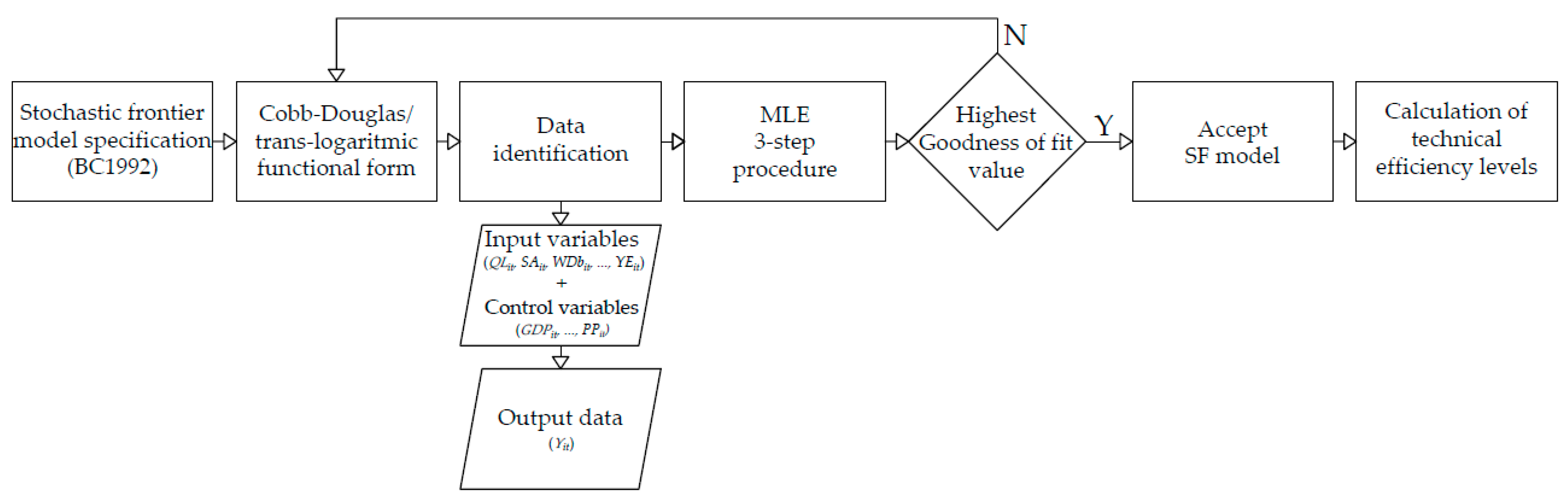
3.1. Theoretical Specification of the Stochastic Frontier Model
3.2. Definition of Output/Input Variables
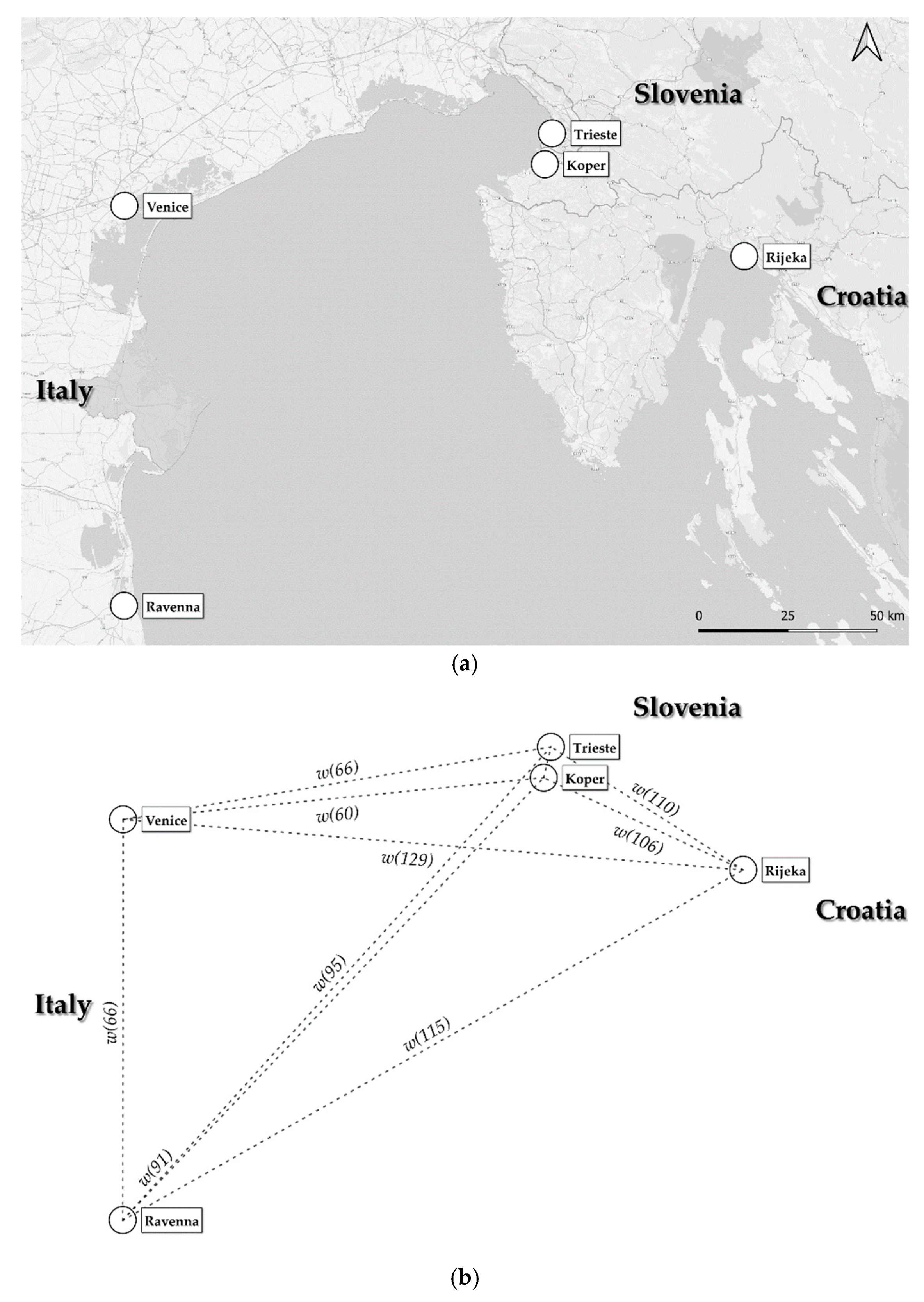
3.3. Testing Area Description and Econometric Models Specification
- : container throughput of the terminal in time period,
- quay length of the terminal in time period,
- stacking area of the terminal in time period,
- water depth of the terminal in time period,
- quay cranes of the terminal in time period,
- yard equipment of the terminal in time period,
- : time trend,
- : country output in time period in which terminal is situated,
- : quantity of traded merchandises (import and export) of the country in period in which terminal is situated,
- : dummy variable which quantifies public/private participation in the ownership structure of the terminal in the time period,
- : vector of unknown parameters,
- each analyzed terminal,
- each analyzed time period,
- : random error term which is identically distributed and independent from ,
- : the technical inefficiency term which is identically distributed as truncations at zero of the .
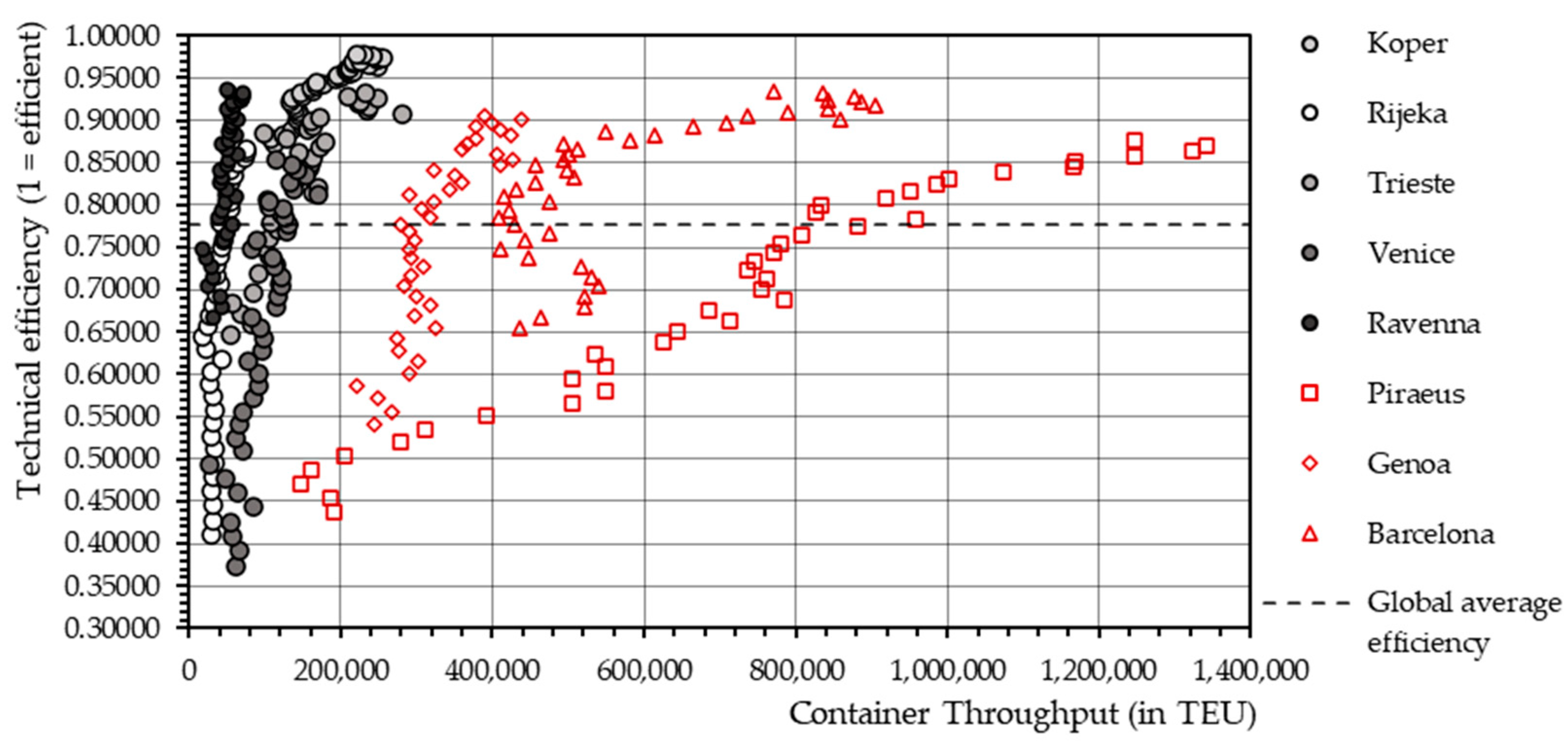
4. Results
5. Discussion
6. Conclusions
Author Contributions
Funding
Data Availability Statement
Conflicts of Interest
References
- Muravev, D.; Rakhmangulov, A.; Hu, H.; Zhou, H. The introduction to system dynamics approach to operational effciency and sustainability of dry port’s main parameters. Sustainability 2019, 11, 2413. [Google Scholar] [CrossRef] [Green Version]
- Merkel, A.; Holmgren, J. Dredging the depths of knowledge: Efficiency analysis in the maritime port sector. Transp. Policy 2017, 60, 63–74. [Google Scholar] [CrossRef]
- Olusegun Onifade, A. New Seaport Development-Prospects and Challenges: Perspectives from Apapa and Calabar Seaports, Nigeria. Logistics 2020, 4, 8. [Google Scholar] [CrossRef] [Green Version]
- Mudronja, G.; Jugović, A.; Škalamera-Alilović, D. Seaports and economic growth: Panel data analysis of EU port regions. J. Mar. Sci. Eng. 2020, 8, 1017. [Google Scholar] [CrossRef]
- Wanke, P.F.; Barbastefano, R.G.; Hijjar, M.F. Determinants of efficiency at major Brazilian port terminals. Transp. Rev. 2011, 31, 653–677. [Google Scholar] [CrossRef]
- Charłampowicz, J.; Mańkowski, C. Economic efficiency evaluation system of maritime container terminals. Ekon. i Prawo 2020, 19, 21. [Google Scholar] [CrossRef] [Green Version]
- Ye, S.; Qi, X.; Xu, Y. Analyzing the relative efficiency of China’s Yangtze River port system. Marit. Econ. Logist. 2020, 22, 640–660. [Google Scholar] [CrossRef] [Green Version]
- Aisha, T.A.; Ouhimmou, M.; Paquet, M. Optimization of container terminal layouts in the seaport-case of Port of Montreal. Sustainability 2020, 12, 1165. [Google Scholar] [CrossRef] [Green Version]
- Tongzon, J.; Heng, W. Port privatization, efficiency and competitiveness: Some empirical evidence from container ports (terminals). Transp. Res. Part A Policy Pract. 2005, 39, 405–424. [Google Scholar] [CrossRef]
- Wilmsmeier, G.; Tovar, B.; Sanchez, R.J. The evolution of container terminal productivity and efficiency under changing economic environments. Res. Transp. Bus. Manag. 2013, 8, 50–66. [Google Scholar] [CrossRef]
- Munim, Z.H. Does higher technical efficiency induce a higher service level? A paradox association in the context of port operations. Asian J. Shipp. Logist. 2020, 36, 157–168. [Google Scholar] [CrossRef]
- Ghiara, H.; Tei, A. Port activity and technical efficiency: Determinants and external factors. Marit. Policy Manag. 2021, 1, 14. [Google Scholar] [CrossRef]
- Pérez, I.; González, M.M.; Trujillo, L. Do specialisation and port size affect port efficiency? Evidence from cargo handling service in Spanish ports. Transp. Res. Part A Policy Pract. 2020, 138, 234–249. [Google Scholar] [CrossRef]
- Pérez, I.; Trujillo, L.; González, M.M. Efficiency determinants of container terminals in Latin American and the Caribbean. Util. Policy 2016, 41, 1–14. [Google Scholar] [CrossRef]
- Siqueira, G.A.; Leal Jr, I.C., Jr.; Cunha, L.C.; Guimarães, V.D.A.; Guabiroba, R.C.D.S. Analysis of technical efficiency and eco-efficiency in container terminals. Int. J. Shipp. Transp. Logist. 2017, 9, 562–579. [Google Scholar] [CrossRef]
- Wiegmans, B.; Witte, P. Efficiency of inland waterway container terminals: Stochastic frontier and data envelopment analysis to analyze the capacity design- and throughput efficiency. Transp. Res. Part A Policy Pract. 2017, 106, 12–21. [Google Scholar] [CrossRef] [Green Version]
- López-Bermúdez, B.; Freire-Seoane, M.J.; Nieves-Martínez, D.J. Port efficiency in Argentina from 2012 to 2017: An ally for sustained economic growth. Util. Policy 2019, 61, 100976. [Google Scholar] [CrossRef]
- Cullinane, K.; Song, D.W.; Gray, R. A stochastic frontier model of the efficiency of major container terminals in Asia: Assessing the influence of administrative and ownership structures. Transp. Res. Part A Policy Pract. 2002, 36, 743–762. [Google Scholar] [CrossRef]
- Notteboom, T.; Coeck, C.; Van Den Broeck, J. Measuring and Explaining the Relative Efficiency of Container Terminals by Means of Bayesian Stochastic Frontier Models. Int. J. Marit. Econ. 2000, 2, 83–106. [Google Scholar] [CrossRef]
- Crisci, A.; Siviero, L.; D’Ambra, L. Technical efficiency with several stochastic frontier analysis models using panel data. Electron. J. Appl. Stat. Anal. 2016, 9, 736–759. [Google Scholar] [CrossRef]
- Cantos, P.; Maudos, J. Regulation and efficiency: The case of European railways. Transp. Res. Part A Policy Pract. 2001, 35, 459–472. [Google Scholar] [CrossRef]
- Yip, T.L.; Sun, X.Y.; Liu, J.J. Group and individual heterogeneity in a stochastic frontier model: Container terminal operators. Eur. J. Oper. Res. 2011, 213, 517–525. [Google Scholar] [CrossRef] [Green Version]
- Suárez-Alemán, A.; Morales Sarriera, J.; Serebrisky, T.; Trujillo, L. When it comes to container port efficiency, are all developing regions equal? Transp. Res. Part A Policy Pract. 2016, 86, 56–77. [Google Scholar] [CrossRef] [Green Version]
- Barros, C.P.; Felício, J.A.; Fernandes, R.L. Productivity analysis of Brazilian seaports. Marit. Policy Manag. 2012, 39, 503–523. [Google Scholar] [CrossRef]
- JimWu, Y.C.; Yuan, C.H.; Goh, M.; Lu, Y.H. Regional Port Productivity in APEC. Sustainability 2016, 8, 689. [Google Scholar] [CrossRef] [Green Version]
- Yang, H.; Lin, K.; Kennedy, O.R.; Ruth, B. Sea-Port Operational Efficiency: An Evaluation of Five Asian Ports Using Stochastic Frontier Production Function Model. J. Serv. Sci. Manag. 2011, 4, 391–399. [Google Scholar] [CrossRef] [Green Version]
- Yang, X.; Yip, T.L. Sources of efficiency changes at Asian container ports. Marit. Bus. Rev. 2019, 4, 71–93. [Google Scholar] [CrossRef]
- Gil-Ropero, A.; Cerban, M.; Turias, I.J. Analysis of the global and technical efficiencies of major Spanish container ports. Int. J. Transp. Econ. 2015, 42, 377–407. [Google Scholar] [CrossRef]
- González, M.M.; Trujillo, L. Efficiency measurement in the port industry: A survey of the empirical evidence. J. Transp. Econ. Policy 2009, 43, 157–192. [Google Scholar]
- Cullinane, K.P.B.; Wang, T.-F. The efficiency of European container ports: A cross-sectional data envelopment analysis. Int. J. Logist. Res. Appl. 2006, 9, 19–31. [Google Scholar] [CrossRef]
- Mortimer, D. Competing Methods for Efficiency Measurement A Systematic Review of Direct DEA vs SFA/DFA Comparisons; Centre for Health Program Evaluation: West Heidelberg, Australia, 2002; Volume 136.
- Serebrisky, T.; Sarriera, J.M.; Suárez-Alemán, A.; Araya, G.; Briceño-Garmendía, C.; Schwartz, J. Exploring the drivers of port efficiency in Latin America and the Caribbean. Transp. Policy 2016, 45, 31–45. [Google Scholar] [CrossRef]
- Almawsheki, E.S.; Shah, M.Z. Technical Efficiency Analysis of Container Terminals in the Middle Eastern Region. Asian J. Shipp. Logist. 2015, 31, 477–486. [Google Scholar] [CrossRef] [Green Version]
- Gamassa, P.K.P.; Chen, Y. Comparison of port efficiency between Eastern and Western African ports using DEA window analysis. In Proceedings of the 14th International Conference on Services Systems and Services Management, ICSSSM 2017, Dalian, China, 16–18 June 2017; pp. 1–6. [Google Scholar]
- Machado de Andrade, R.; Lee, S.; Lee, P.T.W.; Kwon, O.K.; Chung, H.M. Port Efficiency Incorporating Service Measurement Variables by the BiO-MCDEA: Brazilian Case. Sustainability 2019, 11, 4340. [Google Scholar] [CrossRef] [Green Version]
- Santiago, J.I.P.; Orive, A.C.; Cancelas, N.G. DEA-Bootstrapping Analysis for Different Models of Spanish Port Governance. J. Mar. Sci. Eng. 2021, 9, 30. [Google Scholar] [CrossRef]
- Quintano, C.; Mazzocchi, P.; Rocca, A. A competitive analysis of EU ports by fixing spatial and economic dimensions. J. Shipp. Trade 2020, 5, 1–19. [Google Scholar] [CrossRef]
- Kammoun, R. The Technical Efficiency of Tunisian Ports: Comparing Data Envelopment Analysis and Stochastic Frontier Analysis Scores. Logist. Sustain. Transp. 2018, 9, 73–84. [Google Scholar] [CrossRef] [Green Version]
- Nguyen, H.O.; Nghiem, H.S.; Chang, Y.T. A regional perspective of port performance using metafrontier analysis: The case study of Vietnamese ports. Marit. Econ. Logist. 2018, 20, 112–130. [Google Scholar] [CrossRef] [Green Version]
- López-Bermúdez, B.; Freire-Seoane, M.J.; González-Laxe, F. Efficiency and productivity of container terminals in Brazilian ports (2008–2017). Util. Policy 2019, 56, 82–91. [Google Scholar] [CrossRef]
- Farrell, M.J. The Measurement of Productive Efficiency. J. R. Stat. Soc. Ser. A 1957, 120, 253–290. [Google Scholar] [CrossRef]
- Aigner, D.; Lovell, C.A.K.; Schmidt, P. Formation and Estimation of Stochastic Frontier Production Function Models. J. Econom. 1977, 6, 21–37. [Google Scholar] [CrossRef]
- Meeusen, W.; van Den Broeck, J. Efficiency Estimation from Cobb-Douglas Production Functions with Composed Error. Int. Econ. Rev. (Philadelphia) 1977, 18, 435–444. [Google Scholar] [CrossRef]
- Battese, G.E.; Coelli, T.J. Frontier Production Functions, Technical Efficiency and Panel Data: With Application to Paddy Farmers in India. J. Product. Anal. 1992, 3, 153–169. [Google Scholar] [CrossRef]
- Battese, G.E.; Corra, G.S. Estimation of a production frontier model: With application to the pastoral zone of Eastern Australia. Aust. J. Agric. Econ. 1977, 21, 169–179. [Google Scholar] [CrossRef] [Green Version]
- Chang, V.; Tovar, B. Efficiency and productivity changes for Peruvian and Chilean ports terminals: A parametric distance functions approach. Transp. Policy 2014, 31, 83–94. [Google Scholar] [CrossRef]
- Chen, H.K.; Chou, H.W.; Hsieh, C.C. Operational and disaggregate input efficiencies of international container ports: An application of stochastic frontier analysis. Int. J. Shipp. Transp. Logist. 2018, 10, 113–159. [Google Scholar] [CrossRef]
- Jarboui, S.; Forget, P.; Boujelben, Y. Efficiency evaluation in public road transport: A stochastic frontier analysis. Transport 2015, 30, 1–14. [Google Scholar] [CrossRef] [Green Version]
- Karlaftis, M.G.; Tsamboulas, D. Efficiency measurement in public transport: Are findings specification sensitive? Transp. Res. Part A Policy Pract. 2012, 46, 392–402. [Google Scholar] [CrossRef]
- Cobb, C.W.; Douglas, P.H. A Theory of Production. Am. Econ. Rev. 1928, 18, 139–165. [Google Scholar]
- Christensen, L.R.; Jorgenson, D.W.; Lau, L.J. Transcendental Logarithmic Production Frontiers. Econometrics 1973, 55, 28–45. [Google Scholar] [CrossRef]
- Venkadasalam, S.; Mohamad, A.; Sifat, I.M. Operational efficiency of shipping companies: Evidence from Malaysia, Singapore, the Philippines, Thailand and Vietnam. Int. J. Emerg. Mark. 2020, 15, 875–897. [Google Scholar] [CrossRef]
- Bichou, K. An empirical study of the impacts of operating and market conditions on container-port efficiency and benchmarking. Res. Transp. Econ. 2013, 42, 28–37. [Google Scholar] [CrossRef]
- Wan, Y.; Yuen, A.C.L.; Zhang, A. Effects of hinterland accessibility on US container port efficiency. Int. J. Shipp. Transp. Logist. 2014, 6, 422–440. [Google Scholar] [CrossRef]
- Cullinane, K.; Song, D.W. A stochastic frontier model of the productive efficiency of Korean container terminals. Appl. Econ. 2003, 35, 251–267. [Google Scholar] [CrossRef]
- Cullinane, K.; Wang, T. The efficiency analysis of container port production using DEA panel data approaches. OR Spectr. 2010, 32, 717–738. [Google Scholar] [CrossRef]
- Dowd, T.J.; Leschine, T.M. Container terminal productivity: A perspective. Marit. Policy Manag. 1990, 17, 107–112. [Google Scholar] [CrossRef]
- Cheon, S.H. Impact of global terminal operators on port efficiency: A tiered data envelopment analysis approach. Int. J. Logist. Res. Appl. 2009, 12, 85–101. [Google Scholar] [CrossRef]
- Iyer, K.C.; Nanyam, V.P.S.N. Technical efficiency analysis of container terminals in India. Asian J. Shipp. Logist. 2020, 37, 61–72. [Google Scholar] [CrossRef]
- Trujillo, L.; González, M.M.; Jiménez, J.L. An overview on the reform process of African ports. Util. Policy 2013, 25, 12–22. [Google Scholar] [CrossRef]
- Cullinane, K.; Song, D.W. Estimating the Relative Efficiency of European Container Ports: A Stochastic Frontier Analysis. Res. Transp. Econ. 2006, 16, 85–115. [Google Scholar] [CrossRef]
- Cullinane, K.; Song, D.W.; Wang, T. The application of mathematical programming approaches to estimating container port production efficiency. J. Product. Anal. 2005, 24, 73–92. [Google Scholar] [CrossRef]
- Figueiredo De Oliveira, G.; Cariou, P. The impact of competition on container port (in)efficiency. Transp. Res. Part A Policy Pract. 2015, 78, 124–133. [Google Scholar] [CrossRef]
- UNCTAD. Available online: https://unctad.org/ (accessed on 8 April 2021).
- EUROSTAT. Available online: https://ec.europa.eu/eurostat (accessed on 8 April 2021).
- Grubisic, N.; Krljan, T.; Maglić, L.; Vilke, S. The Microsimulation Model for Assessing the Impact of Inbound Traffic Flows for Container Terminals Located near City Centers. Sustainability 2020, 12, 9478. [Google Scholar] [CrossRef]
- Coelli, T. A Guide to FRONTIER Version 4.1: A Computer Program for Stochastic Frontier Production and Cost Function Estimation. In CEPA Working Papers; University of Queensland: St. Lucia, Australia, 2014; Volume 7, pp. 1–33. [Google Scholar]
- Tovar, B.; Wall, A. Specialisation, diversification, size and technical efficiency in ports: An empirical analysis using frontier techniques. Eur. J. Transp. Infrastruct. Res. 2017, 17, 279–303. [Google Scholar] [CrossRef]
- Grubisic, N.; Krljan, T.; Maglic, L. The Optimization Process for Seaside Operations at Medium-Sized Container Terminals with a Multi-Quay Layout. J. Mar. Sci. Eng. 2020, 8, 891. [Google Scholar] [CrossRef]
- Barykin, S.Y.; Kapustina, I.V.; Sergeev, S.M.; Yadykin, V.K. Algorithmic foundations of economic and mathematical modeling of network logistics processes. J. Open Innov. Technol. Mark. Complex. 2020, 6, 189. [Google Scholar] [CrossRef]
- Marmolejo-Saucedo, J.A. Design and Development of Digital Twins: A Case Study in Supply Chains. Mob. Netw. Appl. 2020, 25, 2141–2160. [Google Scholar] [CrossRef]


| NAPA Terminal | Regulator | Landowner | Operator | Value/Function |
|---|---|---|---|---|
| Rijeka | Public | Public | Private | 0.33 |
| Koper | Public | Public | Public | 0.00 |
| Trieste | Public | Public | Private | 0.33 |
| Venice | Public | Private | Private | 0.66 |
| Ravenna | Public | Public | Private | 0.33 |
| Variable Classification | Variables | Unit | Mean | Median | Std. Deviation | Minimum | Maximum |
|---|---|---|---|---|---|---|---|
| Output | Cont. Throughput | TEU | 104,153.51 | 85,254.50 | 66,050.95 | 17,798.00 | 280,637.00 |
| Input | Quay Length | Meters | 722.92 | 649.00 | 203.66 | 300.00 | 1,072.00 |
| Stacking Area | Sq. meters | 120,472.00 | 104,450.00 | 49,730.42 | 60,400.00 | 208,000.00 | |
| Water Depth | Meters | 13.58 | 14.04 | 2.72 | 10.00 | 18.00 | |
| Quay Cranes | No. | 6.12 | 7.00 | 2.20 | 2.00 | 10.00 | |
| Yard Equipment | No. | 74.38 | 64.00 | 28.69 | 37.00 | 131.00 |
| Variable Classification | Variables (Unit) | Unit | Mean | Median | Std. Deviation | Minimum | Maximum |
|---|---|---|---|---|---|---|---|
| Output | Cont. Throughput | TEU | 270,172.95 | 161,644.50 | 276,494.73 | 17,798.00 | 1,342,400.00 |
| Input | Quay Length | Meters | 1063.16 | 921.00 | 523.38 | 300.00 | 2847.00 |
| Stacking Area | Sq. meters | 224,819.41 | 172,000.00 | 148,093.66 | 60,400.00 | 496,100.00 | |
| Water Depth | Meters | 14.40 | 14.94 | 2.66 | 10.00 | 19.50 | |
| Quay Cranes | No. | 9.72 | 8.00 | 6.23 | 2.00 | 31.00 | |
| Yard Equipment | No. | 106.36 | 100.00 | 53.42 | 37.00 | 233.00 |
| Variables | |||
|---|---|---|---|
| Constant | 3.7335 *** (1.2465) | 4.8314 (4.3176) | |
| 0.4240 *** | 0.5823 *** | ||
| (0.1361) | (0.1002) | ||
| 0.7849 *** (0.0829) | 0.8467 *** (0.1267) | ||
| 0.5288 *** (0.1600) | 0.2830 ** (0.1279) | ||
| 0.1506 (0.1045) | 0.3249 * (0.1957) | ||
| 0.6735* * | 0.4713 *** | ||
| (0.2618) | (0.1073) | ||
| 0.1841 *** | 0.2113 * | ||
| (0.0461) | (0.1091) | ||
| 0.2520 *** (0.0579) | |||
| −0.0019 (0.0208) | |||
| 0.1918 *** (0.03386) | |||
| −0.1995* ** (0.03663) | |||
| −0.2971 *** (0.1034) | |||
| 0.1050 * (0.0613) | |||
| −0.6294 *** (0.0554) | |||
| 0.3138 *** (0.0423) | |||
| 0.0758 (0.0767) | |||
| −0.0128 (0.0362) | |||
| −0.0916 ** (0.0363) | |||
| −0.4069 *** (0.0587) | |||
| 0.1003 * (0.0546) | |||
| 0.1217 (0.0797) | |||
| 0.3234 *** (0.0732) | |||
| −0.0077 (0.0312) | −0.0069 (0.0127) | ||
| 0.2763 *** (0.1332) | 0.2981 *** (0.1086) | ||
| 0.3340 *** (0.1400) | 0.3471*** (0.1212) | ||
| 0.4465 ** (0.2199) | 0.4559 ** (0.2271) | ||
| 0.8549 | 0.9463 | ||
| 0.8025 | 0.7411 | ||
| 0.6525 | 0.8699 | ||
| Log-likelihood | 53.3940 | 118.5438 | |
| LR value | 132.3914 | 134.1543 | |
| Time Period (Year) | Time Resolution (Quartal) | Rijeka | Koper | Trieste | Venice | Ravenna | Piraeus | Genova | Barcelona |
|---|---|---|---|---|---|---|---|---|---|
| 2010 | Q1 | 0.4110 | 0.8724 | 0.6459 | 0.3743 | 0.6680 | 0.4372 | 0.5410 | 0.6551 |
| Q2 | 0.4280 | 0.8778 | 0.6589 | 0.3916 | 0.6804 | 0.4541 | 0.5565 | 0.6679 | |
| Q3 | 0.4450 | 0.8830 | 0.6716 | 0.4087 | 0.6925 | 0.4708 | 0.5716 | 0.6804 | |
| Q4 | 0.4618 | 0.8880 | 0.6839 | 0.4258 | 0.7042 | 0.4873 | 0.5864 | 0.6925 | |
| 2011 | Q1 | 0.4784 | 0.8928 | 0.6959 | 0.4428 | 0.7156 | 0.5036 | 0.6009 | 0.7042 |
| Q2 | 0.4949 | 0.8975 | 0.7076 | 0.4596 | 0.7266 | 0.5197 | 0.6151 | 0.7156 | |
| Q3 | 0.5111 | 0.9019 | 0.7188 | 0.4763 | 0.7373 | 0.5355 | 0.6289 | 0.7266 | |
| Q4 | 0.5270 | 0.9062 | 0.7298 | 0.4927 | 0.7477 | 0.5510 | 0.6424 | 0.7373 | |
| 2012 | Q1 | 0.5427 | 0.9102 | 0.7404 | 0.5090 | 0.7577 | 0.5663 | 0.6555 | 0.7477 |
| Q2 | 0.5581 | 0.9141 | 0.7506 | 0.5250 | 0.7674 | 0.5812 | 0.6683 | 0.7577 | |
| Q3 | 0.5732 | 0.9179 | 0.7605 | 0.5407 | 0.7767 | 0.5958 | 0.6808 | 0.7673 | |
| Q4 | 0.5880 | 0.9215 | 0.7701 | 0.5561 | 0.7857 | 0.6101 | 0.6929 | 0.7767 | |
| 2013 | Q1 | 0.6025 | 0.9249 | 0.7794 | 0.5713 | 0.7945 | 0.6241 | 0.7046 | 0.7857 |
| Q2 | 0.6166 | 0.9282 | 0.7883 | 0.5861 | 0.8029 | 0.6377 | 0.7160 | 0.7945 | |
| Q3 | 0.6304 | 0.9314 | 0.7970 | 0.6006 | 0.8110 | 0.6510 | 0.7270 | 0.8029 | |
| Q4 | 0.6439 | 0.9344 | 0.8053 | 0.6148 | 0.8188 | 0.6639 | 0.7377 | 0.8110 | |
| 2014 | Q1 | 0.6570 | 0.9373 | 0.8133 | 0.6287 | 0.8263 | 0.6765 | 0.7481 | 0.8188 |
| Q2 | 0.6698 | 0.9401 | 0.8210 | 0.6422 | 0.8336 | 0.6887 | 0.7581 | 0.8263 | |
| Q3 | 0.6822 | 0.9427 | 0.8285 | 0.6553 | 0.8405 | 0.7006 | 0.7678 | 0.8336 | |
| Q4 | 0.6942 | 0.9453 | 0.8356 | 0.6682 | 0.8472 | 0.7121 | 0.7771 | 0.8405 | |
| 2015 | Q1 | 0.7059 | 0.9477 | 0.8425 | 0.6806 | 0.8537 | 0.7232 | 0.7861 | 0.8472 |
| Q2 | 0.7173 | 0.9500 | 0.8492 | 0.6927 | 0.8599 | 0.7341 | 0.7948 | 0.8537 | |
| Q3 | 0.7283 | 0.9523 | 0.8556 | 0.7045 | 0.8659 | 0.7445 | 0.8032 | 0.8599 | |
| Q4 | 0.7389 | 0.9544 | 0.8617 | 0.7159 | 0.8716 | 0.7547 | 0.8113 | 0.8659 | |
| 2016 | Q1 | 0.7493 | 0.9564 | 0.8676 | 0.7269 | 0.8771 | 0.7644 | 0.8192 | 0.8716 |
| Q2 | 0.7592 | 0.9584 | 0.8732 | 0.7376 | 0.8824 | 0.7739 | 0.8267 | 0.8771 | |
| Q3 | 0.7689 | 0.9603 | 0.8787 | 0.7480 | 0.8875 | 0.7831 | 0.8339 | 0.8824 | |
| Q4 | 0.7782 | 0.9620 | 0.8839 | 0.7580 | 0.8923 | 0.7919 | 0.8409 | 0.8875 | |
| 2017 | Q1 | 0.7872 | 0.9637 | 0.8889 | 0.7677 | 0.8970 | 0.8004 | 0.8476 | 0.8923 |
| Q2 | 0.7959 | 0.9654 | 0.8937 | 0.7770 | 0.9015 | 0.8086 | 0.8540 | 0.8970 | |
| Q3 | 0.8042 | 0.9669 | 0.8983 | 0.7861 | 0.9058 | 0.8165 | 0.8602 | 0.9015 | |
| Q4 | 0.8123 | 0.9684 | 0.9028 | 0.7948 | 0.9099 | 0.8241 | 0.8662 | 0.9058 | |
| 2018 | Q1 | 0.8201 | 0.9698 | 0.9070 | 0.8032 | 0.9138 | 0.8315 | 0.8719 | 0.9099 |
| Q2 | 0.8276 | 0.9712 | 0.9111 | 0.8113 | 0.9176 | 0.8385 | 0.8774 | 0.9138 | |
| Q3 | 0.8348 | 0.9725 | 0.9150 | 0.8191 | 0.9212 | 0.8453 | 0.8827 | 0.9176 | |
| Q4 | 0.8417 | 0.9737 | 0.9187 | 0.8266 | 0.9247 | 0.8518 | 0.8877 | 0.9212 | |
| 2019 | Q1 | 0.8484 | 0.9749 | 0.9223 | 0.8339 | 0.9280 | 0.8581 | 0.8926 | 0.9247 |
| Q2 | 0.8548 | 0.9761 | 0.9257 | 0.8408 | 0.9312 | 0.8642 | 0.8972 | 0.9280 | |
| Q3 | 0.8610 | 0.9771 | 0.9290 | 0.8475 | 0.9342 | 0.8700 | 0.9017 | 0.9312 | |
| Q4 | 0.8669 | 0.9782 | 0.9321 | 0.8540 | 0.9372 | 0.8755 | 0.9060 | 0.9342 |
| Time Resolution (Quartal) | Rijeka | Koper | Trieste | Venice | Ravenna | Piraeus | Genova | Barcelona |
|---|---|---|---|---|---|---|---|---|
| Q1 | 0.6602 | 0.9350 | 0.8103 | 0.6338 | 0.8232 | 0.6785 | 0.7468 | 0.8157 |
| Q2 | 0.6722 | 0.9379 | 0.8179 | 0.6464 | 0.8303 | 0.6901 | 0.7564 | 0.8232 |
| Q3 | 0.6839 | 0.9406 | 0.8253 | 0.6587 | 0.8373 | 0.7013 | 0.7658 | 0.8303 |
| Q4 | 0.6953 | 0.9432 | 0.8324 | 0.6707 | 0.8439 | 0.7122 | 0.7749 | 0.8373 |
Publisher’s Note: MDPI stays neutral with regard to jurisdictional claims in published maps and institutional affiliations. |
© 2021 by the authors. Licensee MDPI, Basel, Switzerland. This article is an open access article distributed under the terms and conditions of the Creative Commons Attribution (CC BY) license (https://creativecommons.org/licenses/by/4.0/).
Share and Cite
Krljan, T.; Grbčić, A.; Hess, S.; Grubisic, N. The Stochastic Frontier Model for Technical Efficiency Estimation of Interconnected Container Terminals. J. Mar. Sci. Eng. 2021, 9, 515. https://0-doi-org.brum.beds.ac.uk/10.3390/jmse9050515
Krljan T, Grbčić A, Hess S, Grubisic N. The Stochastic Frontier Model for Technical Efficiency Estimation of Interconnected Container Terminals. Journal of Marine Science and Engineering. 2021; 9(5):515. https://0-doi-org.brum.beds.ac.uk/10.3390/jmse9050515
Chicago/Turabian StyleKrljan, Tomislav, Ana Grbčić, Svjetlana Hess, and Neven Grubisic. 2021. "The Stochastic Frontier Model for Technical Efficiency Estimation of Interconnected Container Terminals" Journal of Marine Science and Engineering 9, no. 5: 515. https://0-doi-org.brum.beds.ac.uk/10.3390/jmse9050515