
Eco-Friendly Speed Control Algorithm Development for Autonomous Vessel Route Planning


1
Intelligent Mechatronics Engineering Department, College of Software Convergence, Sejong University, Seoul 05006, Korea
2
Korea Research Institute of Ship and Ocean Engineering, Autonomous & Intelligent Maritime Systems Research Division, Daejeon 34103, Korea
3
Fluid Dynamics R&D, Ship and Ocean R&D Institute, Daewoo Shipbuilding and Marine Engineering Group, Siheung-Si 15011, Korea
*
Author to whom correspondence should be addressed.
J. Mar. Sci. Eng. 2021, 9(6), 583; https://0-doi-org.brum.beds.ac.uk/10.3390/jmse9060583
Submission received: 3 April 2021
/
Revised: 14 May 2021
/
Accepted: 17 May 2021
/
Published: 28 May 2021
(This article belongs to the Special Issue Marine Alternative Fuels and Environmental Protection)
Abstract
:The upcoming autonomous vessel voyage is promising future in the maritime sector. However, so far, the contemporary route decision making technologies rely on human intervention. Therefore, this manuscript proposes the two newly developed speed algorithms: the modified fixed speed control and the wave feed forward speed control in the route decision making procedure for the autonomous vessels. These two algorithms can control the vessel’s speed without human intervention in eco-friendly and economic manner. The first algorithm is the wave feed forward speed control that can predict the speed change according to wave loads and compensate it to reduce the fluctuation of speed, power, and fuel consumption. To develop this algorithm, the real time modeling of the wave added resistance and the wave real time effect on propulsion are analyzed. The efficacy of the developed wave feed forward scheme is validated using the in-house route optimization simulation program through comparisons with the results of conventional speed governor control case. The developed schemes are applied to a 173 K LNG (Liquefied Natural Gas) carrier with twin propulsion. The other proposed speed control algorithm is the modified fixed control algorithm. This algorithm improves the conventional fixed power control algorithm by adding a time marching module to satisfy the required time arrival of the voyage. The two proposed methods are analyzed in the various simulations—ideal environmental conditions and real voyage environments: The Pacific and the Atlantic cases. Based on the results, the suggested methods can reduce fuel oil consumption, gas emission, and wear and tear problem of the propulsion devise of ship. In the study, it is clearly demonstrated that the developed wave feed forward speed control and modified fixed power scheme perform much better than the conventional speed governor control case.
1. Introduction
1.1. Motivation
Digitalization, decarbonization, and autonomy are the upcoming technology improvement in a maritime industry. The maritime industry is focused on this efficiency improvement by using these emerging technologies. In the case of decarbonization, these technologies help the international organization and the local country government drive to minimize and regulate the green-house-gas emission. In addition to the Paris and Kyoto convention, the recent IMO 2020 sulfur limitation regulation is among the evidence of environment change agreements. The United States will be back in the protocol then it is one of primary agenda for the global community. The maritime time industry is relatively carbon-efficient in terms of gas emissions compared to the air and road transportation sector. According to IMO GHG (Green House Gas) study [1], a maritime industry contributes to almost 15% of the global gas emission in transportation. IMO has strict non-compliance regulations for the new CO2 reduction regulation. Additional penalties would be imposed to the vanned company. Accordingly, it adds to the operating cost expenditure. Maritime transport generates about one billion ton of CO2 annually. The freight competition in the shipping market has been intensified due to the worsened economic situation due to the COVID-19 pandemic and it is expected to prolong on that account. It is only natural for shipping companies to improve their operation efficiency in terms of navigation, including fuel efficiency and gas emission efficiency.
In 2018, the IMO (International Maritime Organization) adopted the MASS (Maritime Autonomous Surface Ship) that is the autonomous vessel for the ocean-going vessel. Until 2025, the IMO will conduct the regulation change scoping work that the autonomous vessel fits to the regulation. Autonomous vessel voyages by themselves without any human intervention. They plan their own route and avoid collision situation. An autonomous vessel routing algorithm needs to be designed as the controllable form of the autonomous vessel because the current route decision making tech relies on it.
This manuscript aims to improve the deficit of the existing speed control algorithm by proposing a new speed control method for autonomous vessel voyage. The algorithm of the current speed control requires human intervention to satisfy the time constraint of the voyage. Due to environmental loads, the gap between ETA (Estimated Time of Arrival) and RTA (Required Time of Arrival) occurs but the current route decision making cannot satisfy time constraints. The representative ways of the current state of the arts are speed governor control and fixed power scheme. At this moment, the problem is that the current route decision making algorithm does not consider autonomous vessel steering, but it is designed to be controlled by human decision-making. There is a huge gap that the current route decision making algorithm applies to the autonomous vessel. This paper aims to propose the route speed control method that achieves both the efficiency and the robustness at the same time by the attenuation of the unnecessary power fluctuation during a voyage. Moreover, the developed method can be applied to autonomous vessels because it is designed so that it is able to control itself in real-time. Two novel speed control methods for autonomous vessels are developed in this study: the modified fixed power and the wave feed forward speed control method. This paper compares the routing efficiency of the proposed methods to that of the conventional human-based steering route decision making.
1.2. Phenomenon and Contribution
In this section, the research question and the phenomenon of the problem that will be solved in the whole manuscript is explained.
1.2.1. Phenomenon
The conventional routing algorithm assumes that the speed command will be maintained as the route commands during the stage that is the unit segment of the route optimization [2]. This assumption is made when selecting the route candidate evaluation and the final speed command. However, in real-world scenarios, the speed is always stumbled without the speed controller due to the environmental load fluctuations such as wave loads. Therefore, the speed governor control is applied to maintain this speed commands that are determined by the routing decision making algorithm. This speed governor controller, basically, does the bull’s eye control scheme therefore the controller keeps the change of the speed even there is a small difference current speed and the target speed. During this procedure, the speed governor controller continuously variates the speed and the power. In consequence, the additional fuel oil consumption, and tear/wear problem in the propulsion component occurred. The difference between the speed governor control and fixed power control method is explained in Equation (1)
- Speed governor control: regulate power based on Vcommand, power = Phull + Penvironment
- Fixed power control: regulated power based on Pcorresponding then V becomes V = Vcommand – Vspeed loss due to environment
As seen in the Figure 1, the speed governor control continuously causes fluctuations in speed and propeller rpm. You [3] proved this phenomenon by the measuring of the 173 K LNGC (Liquefied Natural Gas Carrier) voyage. Therefore, the most ships adopt the fixed power control rather than the speed governor control. However, the disadvantage of the fixed power is that the fixed power method cannot satisfy the required time arrival constraint of the voyage due to the fluctuation of the speed. Generally, the fixed power control schemed needs the captain catch up in the last few voyage stages. This catching up operation also consumes additional fuel. Therefore, the current navigation route decision making procedure has two main disadvantages. Generally, the captain covers this grey zone. This phenomenon needs to be improved to enhance the efficiency of conventional vessels and the applicability to autonomous vessels. For autonomous vessels, the routing algorithm has the key steering algorithm that controls the vessel’s heading and speed during the navigation. Therefore, it is necessary to investigate the best approach to develop a routing algorithm that controls the vessel’s navigation in an efficient manner and the navigation constraint satisfaction. This study investigates the best way to control speed for autonomous vessel and how much the ship’s key performance change according to the speed control schemes. This research proposed two new speed control methods that target autonomous vessel voyage. The voyage performance of the two proposed speed controls is compared to the state of the arts: speed governor control. In 1.3, the state of arts for the vessel speed control is reviewed and the proposed methods are described.
1.2.2. Contribution
This research contributes in two respects compared to previous route optimization algorithm. First, the two speed control algorithms, i.e., modified fixed speed control and wave feed forward speed control, are proposed. These methods can save more fuel and satisfy the arrival time constraint without human intervention for autonomous vessel operation. Second, this study models and analyzes the time domain effects of the environmental loads on propulsion performance of the ship. In Kim’s [4,5], Paratap’s [6], and Pacheco’s [7] research on conventional routing algorithms, the routing algorithm is based on the assumption that the command speed will be maintained in the unit’s stage of the route. This assumption can be achieved when a speed governor control is employed. However, the speed governor control consumes more fuel, emits more green-house gas, and causes a wear and tear problem in the engine and shaft. Although a fixed power fixed speed control scheme is generally adopted in real-world voyages, it cannot satisfy the time constraint of the routing due to speed reduction by the environmental loads.
Additionally, [4,5,6,7] did not consider the variation of the propulsion performance due to time domain effects of the wave loads. In other words, the previous research threats thrust deduction, wake, thrust, and torque as the averaged value without considering the environmental loads. Conversely, the current research models the time domain variation of the propulsion performance due to the wave loads. This modeling achieves an accurate propulsion performance estimation.
1.3. State of the Arts
1.3.1. Route Decision Making Algorithm
In the last decade, ship route decision making research generated a lot of interest because of high fuel price and the competitive nature of shipping industry. Among the various aspects investigated, researches are categorized in to two main streams, that is, the optimization method and the accurate ship performance prediction in the route decision making procedure [2,4]. The route decision making research presumably gets more intension from researchers’ because the route decision making system of its potential as the navigation algorithm for the impending autonomous vessel.
The mainstream of the route decision making research focuses on the route optimization algorithm development. The state of the arts of routing optimization is three-dimensional dynamic programming that evaluates and simulates the route candidates in three dimensions: latitude, longitude, and speed. The principal of the dynamic programming involves dividing complicated optimization problems into unit small segments and finding the solution of each segment. Accordingly, the combination of each segment gives the solution of whole complicated problem. Kim [5] and Vettor [8] tried to model the ship performance appropriately and improved the 3DDP (Three-Dimensional Dynamic Programming) method. Generally, the route decision making set the single object function as the fuel oil consumption to preserve the efficiency of the voyage while satisfying the safety constraint. Multi-objective route optimization is also researched [9].
The other stream for the routing research is the ship performance modeling research. Generally, almost the whole ship performance is modeled to realize the ship routing problem, such as resistance, propulsion, and environmental loads. Therefore, the route decision making action would be based on the precise ship performance modeling. There are many studies that model the ship performance into route decision making procedures [5]. There are many efforts to consider while evaluating the ship’s routing performance. The research in [7] targets ship’s seakeeping performance. Kwon’s [10] work focused on the ship speed loss due to environmental loads. You [3] proved the difference of the speed estimation prediction based on speed, rpm, and power by using real-measurement data of the voyage [3]. Kim’s work [4] focus on modelling the actual ship performance for routing optimization. Pennino [11] suggests a new method to model weather impact in the route decision making problem. Comparison of the estimation model and the actual measurement by using real-sea operation data is done. Another interesting approach is the ship performance estimation based on the deep learning based by actual measurement data. Yan [12] and Du [13] adopted ANN (Artificial Neural Network) to predict the fuel oil consumption performance based on operation data. These approaches promise the practical way when ship design is hard to get for the analysis.
1.3.2. Speed Control Algorithm in Route Decision Making
The optimal speed for shipping has been studied for many decades. Paraftis [14] present the state of the speed model in maritime shipping, and Venturini [15] propose the speed optimization speed under the multi berth problem. Additionally, Zhang [16] and Zis [17] overview the current routing method in the maritime trade supply chain.
This manuscript focuses how to control the speed of the ship under given speed command of the voyage planning. Conventional control scheme for mechanical propulsion with a fixed pitch propeller involves the control speed as a function of the lever setting. This control scheme sets the speed and the engine generate the power that corresponds to the lever setting however power is always variated due to external disturbances such as environmental loads. Vessel and vessel’s propulsion system would like to maintain a given command speed. The engine’s speed governor generally fulfils this task by using a PID controller. Many studies have conducted speed control that has caused unnecessary engine load disturbances. It is natural that the vessel’s speed remains unstable due to environmental load fluctuations, but the PID-based speed governor continuously works like bull’s eye control. Furthermore, the power and fuel oil consumption endlessly fluctuated when the route decision making algorithm adopts the speed governor control as a result of environmental loads. Faber [18] also argues that the time-varying engine load causes fluctuation in fuel injection leading to changed thermal load, which results in bad fuel efficiency. However, the maritime industry generally uses speed governor control because it guarantees the required time arrival.
Propulsion power steady control is the method that controls power steadily. If the controller keeps the power steady, then the vessel speed is varied due to external disturbances. The advantage of this control scheme is that it reduces unnecessary engine power variation that is the main contributor of additional fuel oil consumption, gas emission, and wear and tear problems in the propulsion system. Especially, the LNGC shaft and propulsion system are not robust in fatigue due to the high frequency operation, thus this control scheme helps to prolong the lifetime of the shaft component. There are many studies that prove this phenomenon. According to Faber’s work [18], the torque and power control can significantly reduce thrust, torque, and power fluctuation in both mechanical and electric drives. Moreover, this power steady control is widely used in the dynamic position control to reduce fuel oil consumption and gas emission. In this study, we selected a steady power control scheme as the one of the possible candidates for the autonomous vessel and smartship routing problem. Accordingly, a comparative analysis with conventional speed governor control method was conducted to explore the applicability of the fixed power control.
2. Materials and Methods
In this section, the theoretical-background, and the overall problem-solving procedure of the proposed speed control scheme for routing is exploited. As a start, the target routing optimization problem is formulated, then the ship performance modeling and the time-varying dynamic effect of the ship are stated. At last, the proposed methods: elucidation of modified fixed power control and wave feed forward control.
2.1. Problem Formulation
In this section, the target problem formulation is described. The target problem is the single objective optimization problem. The objective function is the integral form of the fuel oil consumption, thus this problem attempts to find the solution that leads the time accumulated fuel oil consumption. The target problem is the journey that finds the optimal propulsion command that minimize the unnecessary fuel oil consumption fluctuation. The objective function and design variable of the problem are presented in Equation (2). Fuel oil consumption modeling is illustrated in Figure 2.
- Design Variable
- Speed governor control: vessel speed and vessel heading;
- Power control: power and vessel heading;
- Wave feed forward control: power and vessel heading;
- Hybrid control: power and vessel heading.
- Constraints
- Geographical constraints;
- Maximum power: engine constraints (low and high limit);
- Power fluctuation;
- Water depth.
2.1.1. Object Function Modeling
The norm of route evaluation and decision-making procedure is the fuel oil consumption therefore its estimation needs to be precisely predicted. The route optimization result and comparative analysis tends to be closer to the real-world scenario when the fuel oil consumption modeling precision is precisely predicted. In this research, the ship performance modeling is structured based on the state of art ship performance modeling, which is based on the theoretical, the model tests, and the sea trial result. The resistance, propulsion, and environmental loads of ship need to be included in the modeling of the fuel consumption. Generally, precise and extensive studies of the ship’s performance is essential to accurately estimate the fuel consumption of vessel. According to Kim’s work [19], the ship performances that cause high fuel consumption are well illustrated. Moreover, his work clarified the relation between fuel oil consumption, power, and green-house gas emission. According to his work, the fuel consumption and CO2 emission are directly proportion to each other. The authors attempted to make the hydrodynamic model precise enough to estimate the fuel consumption well the actual sea voyage. In this research, the representative 173,000 m3 LNG carrier’s engine, propulsion, ship response and environmental model test data are referred to in [4,5]. This vessel utilized is a standard LNGC plies all ocean routes. Especially, it would be utilized well in the upcoming the LNG exchange between Asia and United States through the Pacific.
Fuel oil consumption is modeled as in Equation (3). Specific fuel consumption is obtained by the characteristic of the engine.
Fuel Oil Consumption(ton) = Required Power × Specific Fuel Oil Consumption
Figure 2 shows the fuel consumption estimation procedure based on the ISO15016:2015 and Holtrop–Mennen method [19]. The FOC Fuel Oil Consumption prediction modeling is based on the resistance and the propulsion model, not on the maneuvering model. The coefficients in the fuel oil consumption estimation are 173,000 m3 LNG Carrier’s. Propulsion data such as the thrust coefficient (KT), the torque coefficient (KQ), the wake coefficient (w), and thrust deduction coefficient (t) can be calculated from the data of the Section 2.1.4. Wind load coefficients and wave quadratic transfer functions in Equations (6) and (7) can be referred Kim [4] model test data. ηD is calculated from the Holtrop–Mennen method.
The required power is defined by multiplication of the engine efficiency, propulsion, and shaft efficiency with the total resistance. The components of total resistance consist of resistances due to the hull itself, wind, and wave. The efficiency of the propeller and shaft are considered in the power calculation.
The details of the propulsion efficiency are described as in Section 2.1.4. Figure 3 shows the specific oil consumption and gas emission of 173 K LNG Carrier’s engine (Table 1).
2.1.2. Resistance Modeling
The speed variation in route decision making is the prime parameter of the resistance that is the main cause of the fuel oil consumption that is the object function route decision making. Fuel oil consumption is mainly caused by the hull and the environmental loads. This modeling is well described in the Kim’s work [4]. However, the dynamic effect modeling in propulsion and resistance due to wave is rarely investigated in his work. This manuscript expands this research area to the consideration of the dynamic environmental effect in the routing. The way of the consideration is to model the first and second order wave loads which are included in the resistance component first and then consider the dynamic effect in the propulsion is considered.
This manuscript includes the first and second order wave loads into resistance and propulsion modeling. The contribution of this work is mainly that the route decision making can measure the ETA change due to wave load variation in time. Moreover, a new speed controller that can attenuate the wave load variation by modeling real-time estimation is proposed. Using this work, the route decision making can satisfy the RTA and ultimately energy-saving voyage is possible compared to the conventional static wave treated route decision making.
Wave real time contribution in Fuel Oil Consumption can be obtained from the convolution form of the wave quadratic information and the available wave real time height information. It is described in detail as in [20] and the following section. Power and resistance could be modeled as shown in Equations (4)–(7)
where Vactual = Vcalm − Vspeed loss due to environment
Rtotal: total resistance, Rcalm: resistance in calm water, Rwave: wave-added resistance, and Rwind: wind resistance.
Ptotal = Pcalm + Penvironment = (Rcalm + Rwind + Rwave)Vactual
Pcalm + Penvironment = (Rcalm + Rwind + Rwave)Vtarget
- VWR and ψWR: relative wind speed and direction, respectively.
2.1.3. Wave Real Time Dynamics Modeling
The wave second order force is the prime factor that needs to be considered in autonomous RDM (Route Decision Making) speed control because it makes the time difference and additional fuel consumption. If it is possible to estimate the real-time second order slowly varying force, then it can be attenuated by counter acting speed control and vessel ultimately can control ETA and ATA (Actual Time of Arrival) without discrepancies due to wave and measure FOC for better route decision making. The real time second order slowly varying wave force is the prime component that results in additional fuel oil consumption during the voyage because it is not zero mean and steadily pushes the hull opposite with advance, thus the second order slowly time varying wave component modeling is a key part to realizing minimal fuel oil consumption voyage. So far, there is no research that applies this real time domain wave second order slowly varying force to route decision making. First, this paper applies the wave second order force modeling to the speed and the power control module for routing optimization. Conventional method treats the wave second order force as the mean drift force concept. Conventional method wave estimation precision is lower than that of Kim’s method by about 30% total amplitude. Moreover, the conventional method cannot calculate the time-varying real time response wave load that is the most critical factor for the ship’s routing performance. The advantage of Kim’s method is that it can calculate the dynamic real time response of the wave added resistance by using the time domain quadratic impulse function with wave height. Wave second order time varying added resistance can be modeled as Equations (8) and (9).
- where F(1)(t): the first order wave force, F(2)(t): the second order wave force.
- t: the present time, τ: time to calculate memory effect, h(τ): the first order impulse function, and h (τ1, τ2): quadratic impulse function.
The wave QIF (Quadratic Impulse Function) h (τ1, τ2) can be obtained from the double inverse Fourier transform of the wave QTF (Quadratic Transfer Function), as shown in Equation (9) [20].
2.1.4. Fuel Oil Consumption and Propulsion Dynamics Change Due to Environmental Loads
Conventionally, the ship propulsion parameters, such as wake, thrust deduction, thrust, and torque coefficients are regarded as static value that are chronically steady, but the propulsion efficiency is time-varying due to wave. This manuscript aims to include time varying ship propulsion performances effect in the fuel oil consumption. Torque, thrust, and engine acceleration and deceleration are all the time varying value under external disturbances. For achieving this aim, the dynamic modeling of the engine and propulsion performance modeling would be described in this section. Figure 4 presents the ship performances are related to the environment. The fuel oil consumption is the result how the environments affect to the propulsion and the engine dynamics of the ship performances.
In previous work, the relation among the power, the propulsion efficiency, the speed, and the fuel oil consumption are modelled just as the static values and not dynamic values, which are more accurate. Therefore, this manuscript includes the dynamic effect of the propulsion efficiency due to environmental loads. Wave component also affects propulsion parameter, such as wake, thrust, and flow attached in the hull. To consider dynamic effect of FOC in real time, the wave real time variation to propulsion should be included.
First, the engine dynamics is rarely explored for dynamic load variation that causes additional fuel oil consumption during the voyage. During the acceleration and deceleration, more fuel oil is consumed compared to when in steady power state. Generally, this aspect is not considered in the power control. However, the frequent deceleration and acceleration results to consumption of additional fuel; therefore, it is an important parameter to be considered. To consider accumulative value of the time varying engine load change, the integration form of the engine dynamics should be considered as in Equation (10).
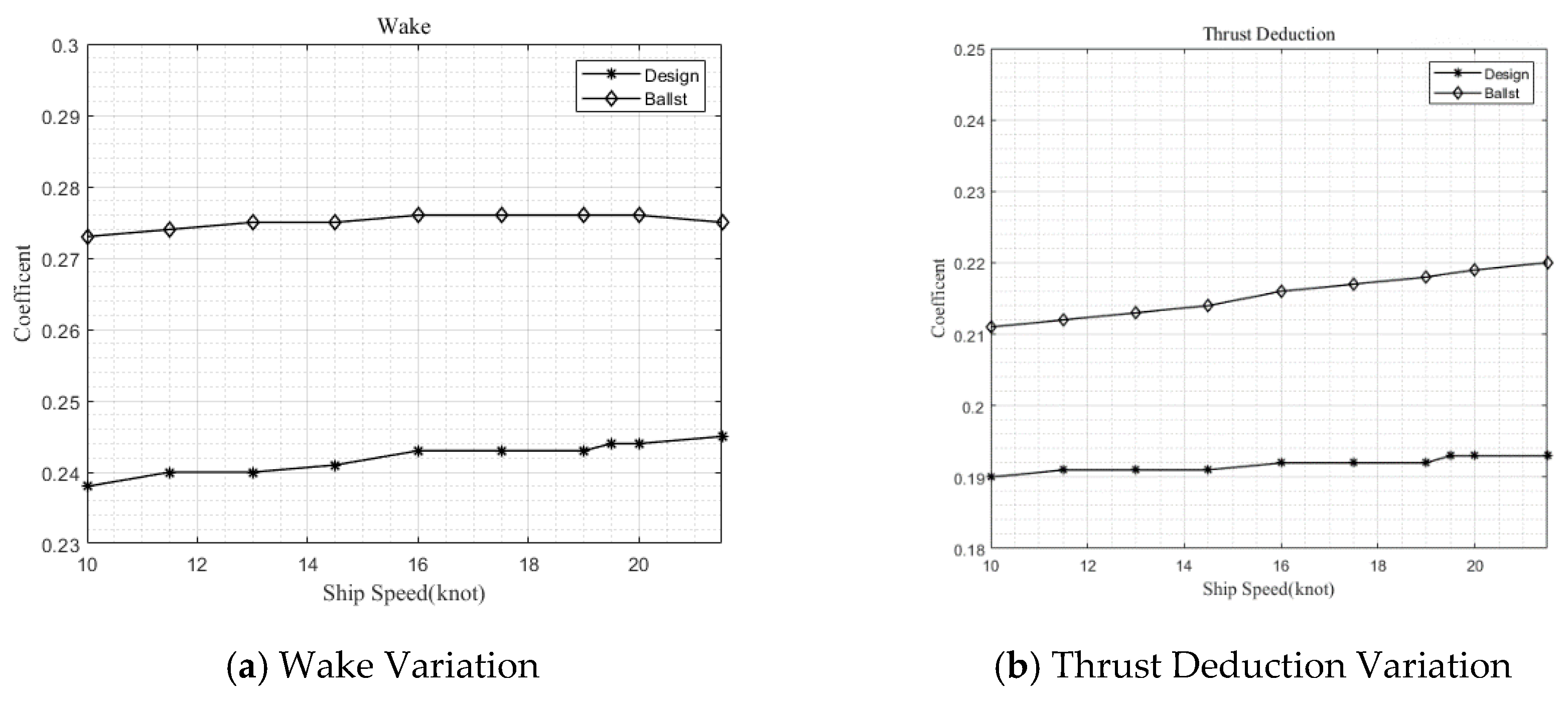
To model the dynamic engine load, thrust and torque coefficient variation due to wave load are included. To include the dynamic term of the wake and thrust are included in the power modeling. Wake and thrust are the time varying parameter that are affected by the vessel’s speed. This paper models the time varying effect due to vessel speed variation as in Figure 5. In Figure 5, design and ballast present the design draft and ballast draft condition of the ship, respectively.
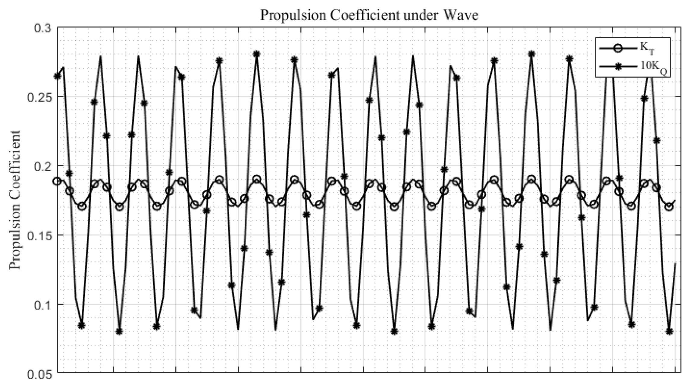
Moreover, the dynamic effect of environmental load on propulsion performance is also another dominant parameter that should be considered. Therefore, among the representative environment parameters: wave is the biggest contributor [21]. The torque and the thrust coefficients fluctuate over various load conditions causing additional fuel oil consumption under waves. According to results [21], the thrust coefficient is fluctuated by 10% and torque coefficient is fluctuated by 33% under wave as in Figure 6.
2.1.5. Routing Decision Making Procedures
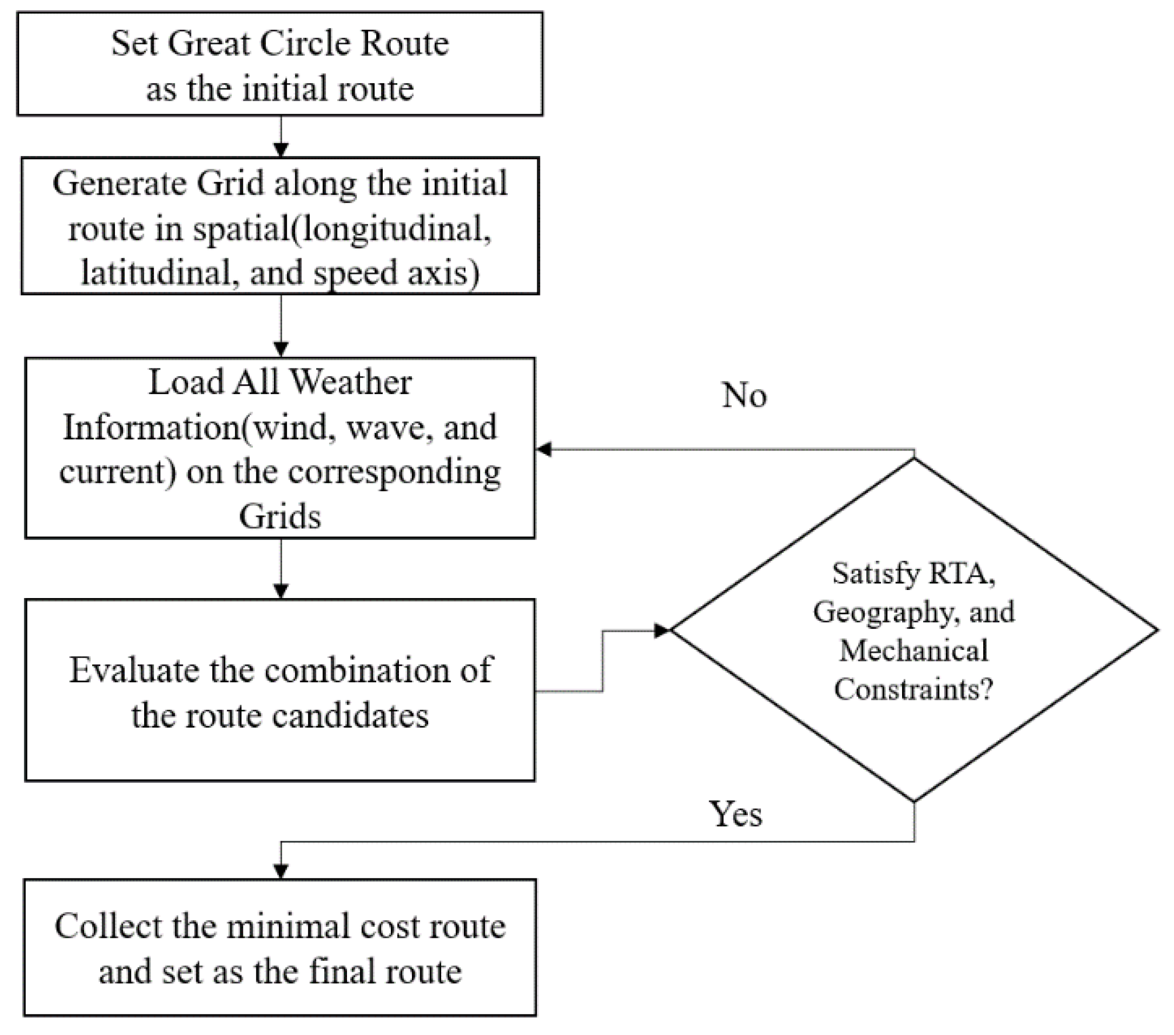
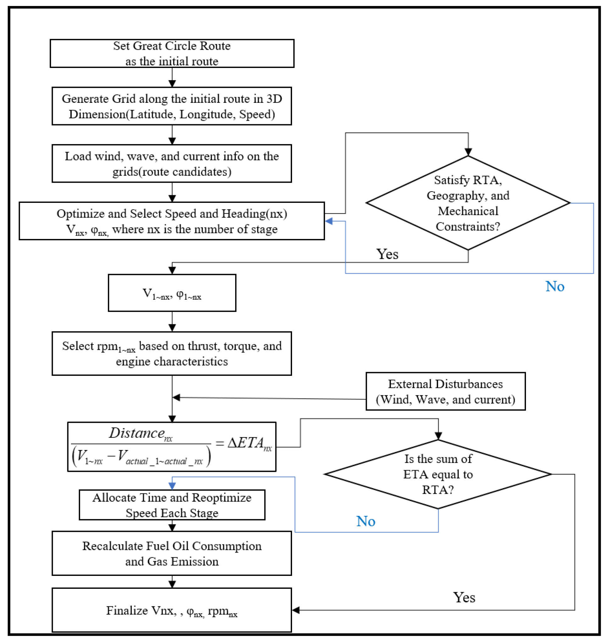
This study improves the speed control algorithm of conventional routing algorithm—3DDP—by satisfying the required time arrival condition and attenuating the fluctuations in power. For this improvement, two methods are proposed—modified fixed power speed control and wave feed forward control. To elaborate on the proposed speed control method, the conventional 3DDP method’s basic procedure is illustrated as in Figure 7.
2.2. Development Speed Control Strategy for Routing Method’s Description
In this section, two newly developed speed control algorithms for the route planning of the autonomous vessel are suggested and their methodologies explained. These two algorithms enhance the accuracy of the route decision making of the autonomous vessel making it more practicable in terms of timely arrival condition and reduced fuel consumption and gas emissions. The newly proposed algorithms are the modified fixed power control and the wave feed-forward speed control. In Section 2.2.1 and Section 2.2.2, the two proposed methods are described in detail.
2.2.1. Modified Fixed Power Speed Control
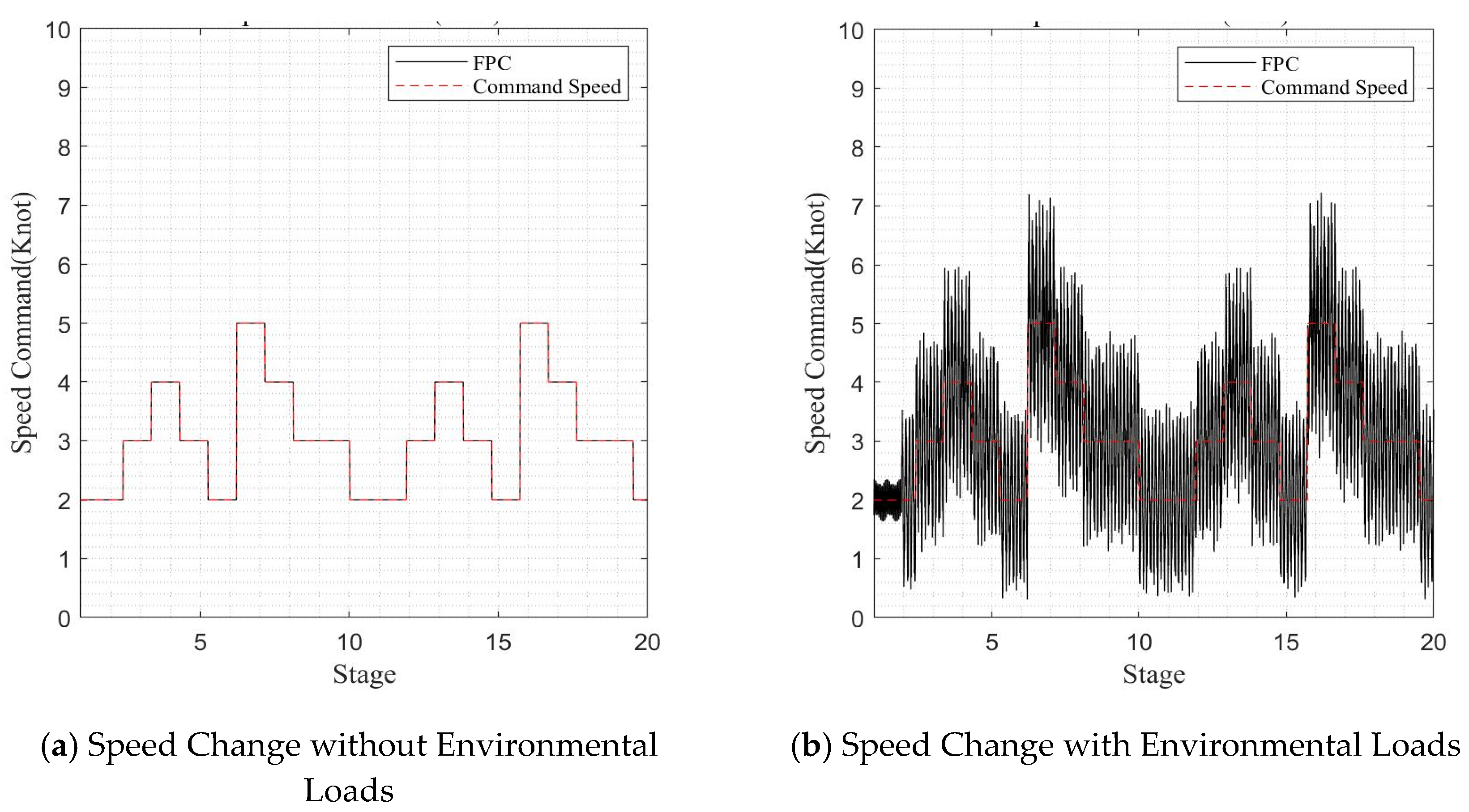
The fixed power speed control scheme issues speed control command to the engine, not as speed but as power that corresponds to command speed. If the environmental load becomes zero, then the control speed is equal to the intended speed of route decision making as in Figure 8.
Fixed power control just maintains the power it can save FOC compared to the speed governor control, but it cannot satisfy RTA because of speed reduction due to environmental loads. The accumulated time arrival discrepancy occurs when the fixed power control is employed. If the captain is on board, then he/she compensates for this discrepancy; thus, an additional compensator is necessary for the smart vessel and the autonomous vessel route decision making.
Moreover, the current route decision making does not consider the fixed power speed control scheme. The current route decision making methodology assumes that the command speed will be maintained during the voyage as the speed control. Therefore, the route decision making does not consider the discrepancy between ETA and RTA.
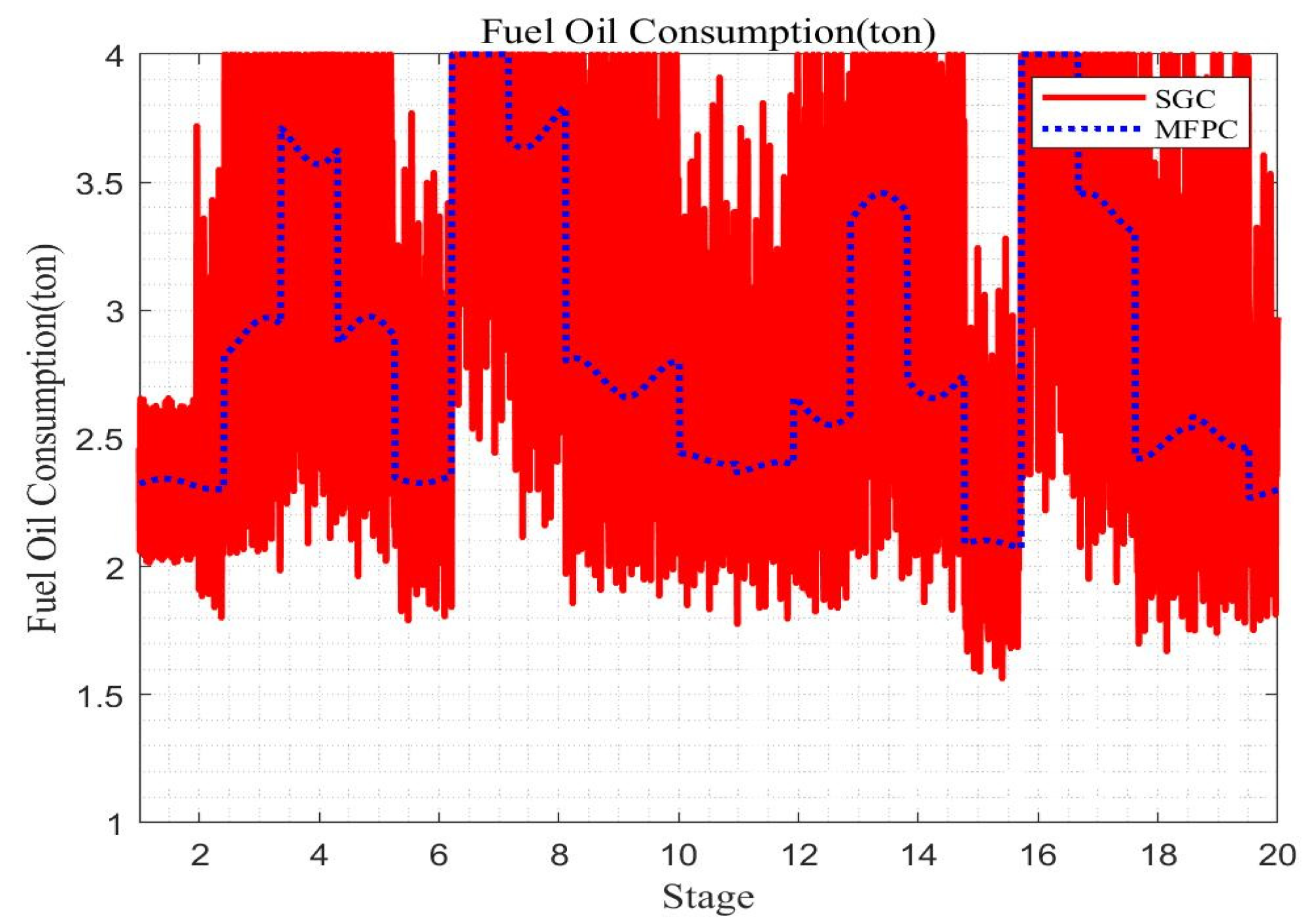
The routing algorithms stabilize the vessel’s speed that naturally fluctuates due to environmental loads. Meanwhile, the fuel oil consumption due to the wave fluctuation are remarkably reduced. Similarly, this steady power control routing cannot satisfy the required time of arrival because the speeds are varied due to environmental loads. This phenomenon results to the difference between the original required time arrival and the required time arrival after the fixed power control is employed. In Figure 9, the red line presents the fuel consumption result due to the adoption of speed governor control and the modified fixed power control. The speed governor control and modified fixed power control are showed by red and blue lines, respectively. In legend, the SGC (Speed Governor Control) denotes speed governor control and the MFPC (Modified Fixed Power Control) denotes modified fixed power control.
The required time arrival difference becomes as seen Equation (11):
The proposed methods add two unique features that calculate the difference between ETA and RTA and allocate this difference into each route stage as like Figure 10. In Figure 10, the required time arrival constraint is evaluated right after the optimal speed is selected. If the required time arrival does not meet, then the routing optimization method selects and optimizes until required time arrival is satisfied. After external disturbances such as wind, wave, and current are calculated, then time marching constraint that judges one more time the agreement of the estimated time arrival and the required time arrival. The calculation of the comparison the optimal routing calculation took 2.7 h by using the author’s computation resources (computation resource: intel i9-10900k CPU, 64 GB RAM).
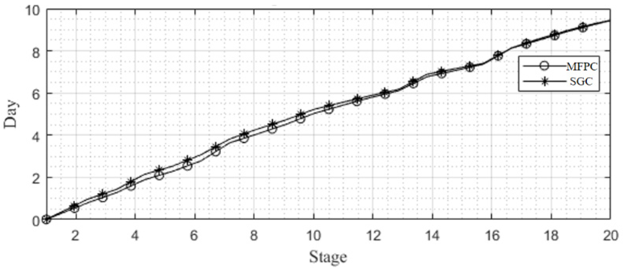
Figure 11 presents the ETA output result of the proposed method. The line with circular marks represents the developed fixed power control and the line with the asterisk mark represents the speed governor control. FPC with time compensator—modified fixed power control—gradually catch up the ETA of speed governor control original fixed power control cannot satisfy the required time arrival, but the developed method finally catches up the required time arrival as in Figure 11.
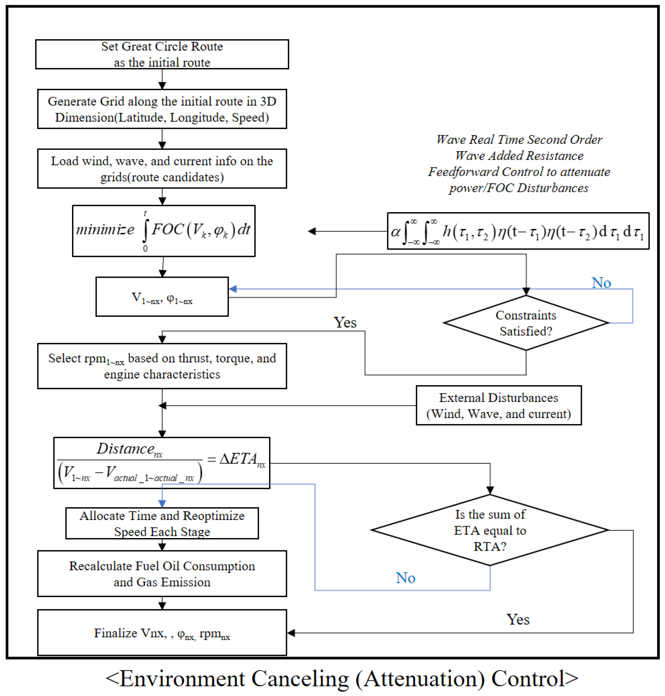
2.2.2. Wave Feed Forward Speed Control
Pre-described fixed power control determines the power through the summation of the hull resistance and the environmental loads. Among the environmental loads, the wave-added resistance is modeled as the mean drift force that lasts longer than 6-h. In other words, it is not accurate whether it caused additional acceleration and deceleration to linearly capture the time constraint.
The proposed method in this section, speed control can attenuate time difference between ETA and RTA due to real-time wave load variation estimation. This can make the result to the optimal operation of the vessel. Namely, it can save fuel oil consumption and GHG compare to fixed power control with a time compensator. In other words, the pre-described fixed power control with compensator can be applied to autonomous vessel route decision making, but wave feed forward attenuation speed control can save more fuel consumption and GHG.
This way cannot capture the dynamic response of the engine load variation due to the wave added resistance fluctuation and causes additional fuel consumption. Consequently, this research proposed a wave feed forward speed control for routing that can compensate for the wave added resistance fluctuation in real-time. The original routing method considered the wave added resistance as the average value during the stage. The conventional method cannot consider the real-time wave added resistance variation, but the proposed wave feed forward method can attenuate this wave added resistance time varying value in a pre-emptively manner, so that the fuel oil consumption is reduced. The key feature of this method includes the cost evaluation of the routing to the wave real time prediction model. The environmental load fluctuation is generally caused by the wave second order slow varying force. In the case of the first order force, it is just a zero mean, thus it does not affect the RTA and fuel consumption. The logical algorithm of the wave feed forward speed control method is presented as in Figure 12.
In cost evaluation, the required power and the fuel oil consumption at stage are modeled as in Equation (3). The wind load is assumed to be in the co-linear direction with wave load. The method can estimate real time wave load are the integral and convolution form of the time-domain wave quadratic and single form of wave impulse function (h). h is varied the wave direction and the vessel speed. h functions could be obtained by the motion analysis as in Equation (8) [20].
3. Results
3.1. Target Vessel
3.2. Ideal Environmental Condition
In this section, the performance of the proposed speed control methods, that is, modified fixed speed control and wave feed forward control are discussed under intentionally designed environmental conditions for the verification of the proposed speed control. Three designed environmental conditions are applied to the route candidate to present the proper performance of the speed control method due to variation of weather. These conditions include mild, medium, and adverse condition. The mild condition is based on the Beaufort 3, the medium condition is the Beaufort 5, and the adverse condition is the Beaufort 7. The simulation results show how the proposed speed control scheme react to various intensities of the environments. The direction of the wind and wave is assumed to be collinear.
The response of the proposed speed control methods are intuitively verified in this section. Table 3 shows the weather scenario of the route and the instances of the corresponding speed commands.
Table 4 shows the example data set for the fuel oil consumption calculation under medium environmental load condition case in stage 2. Figure 2 explains the procedure of the FOC estimation that includes the example data of Table 5. Table 5 illustrates how the reader can reproduce the result of the fuel oil consumption modeling for the target vessel—173,000 m3 LNG Carrier.
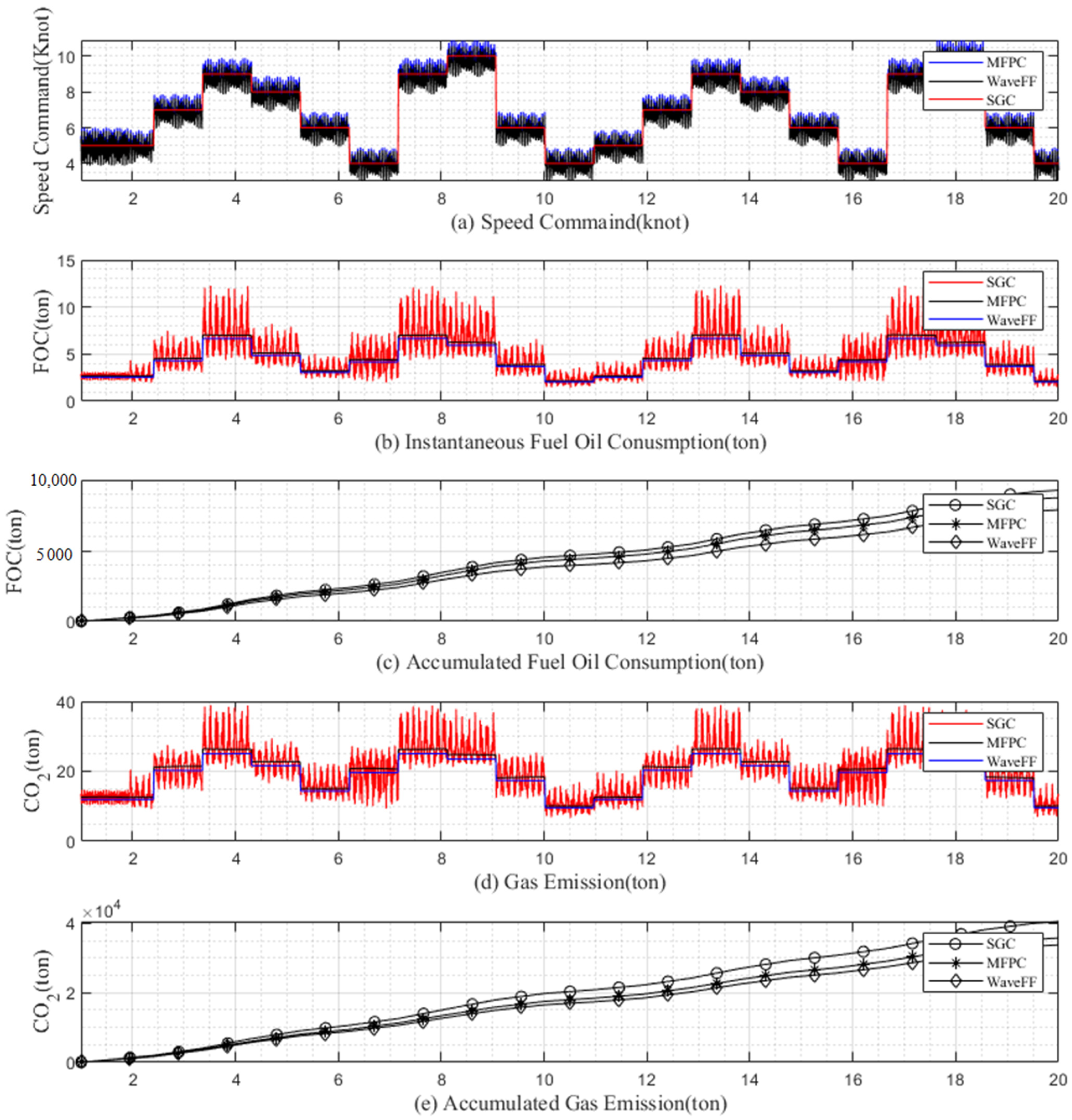
Figure 14 shows the speed, the instantaneous fuel consumption, and cumulative fuel oil consumption time step according to the stage of the voyage. The X axis represents the stage of the voyage. The red line presents speed governor control, blue colored line represents the modified fixed power control, and black lines represent wave feed forward speed control. As seen in Figure 14, the vessel speed fluctuates due to environmental conditions. The speed governor control clearly shows the effect of the environmental load on the vessel voyage speed. The additional perturbation is found when the speed governor control is employed in the instantaneous fuel oil consumption of the voyage. Consequently, these unstable fluctuations consume more fuel compared to the instance of accumulated fuel.
In the case of the fuel oil consumption, the wave feed forward speed control shows the best performance in the instantaneous and the accumulative value. The speed governor control causes the high fluctuation in the instantaneous fuel oil consumption and results the largest fuel oil consumption in time-accumulative regards. In the legends of Figure 14, FPC, SGC, MFPC, and WaveFF denotes the fixed power control method, the speed governor control method, the modified fixed power control, and the modified wave feed control method, respectively.
Table 6 shows the relative fuel oil consumption due to the application of modified fixed power and wave feed forward control method to the conventional speed governor control method. The absolute value of fuel oil consumption cannot be included because the fuel oil consumption data is confidential. Comparing the speed governor control, the modified fixed power, and the wave feed forward, the latter shows the best performance in reducing the instantaneous and accumulated fuel oil consumption. It achieved a noticeable amount of fuel saving compared to the conventional fixed speed control method. The fixed speed control strategy causes a continuous fluctuation in the fuel oil consumption. Consequently, this frequent fluctuation causes wear and tear problem in the engine and propulsion driving system. In worst cases, wear and tear problem can result to down time for the ship.
4. Discussion
4.1. Pacific Case
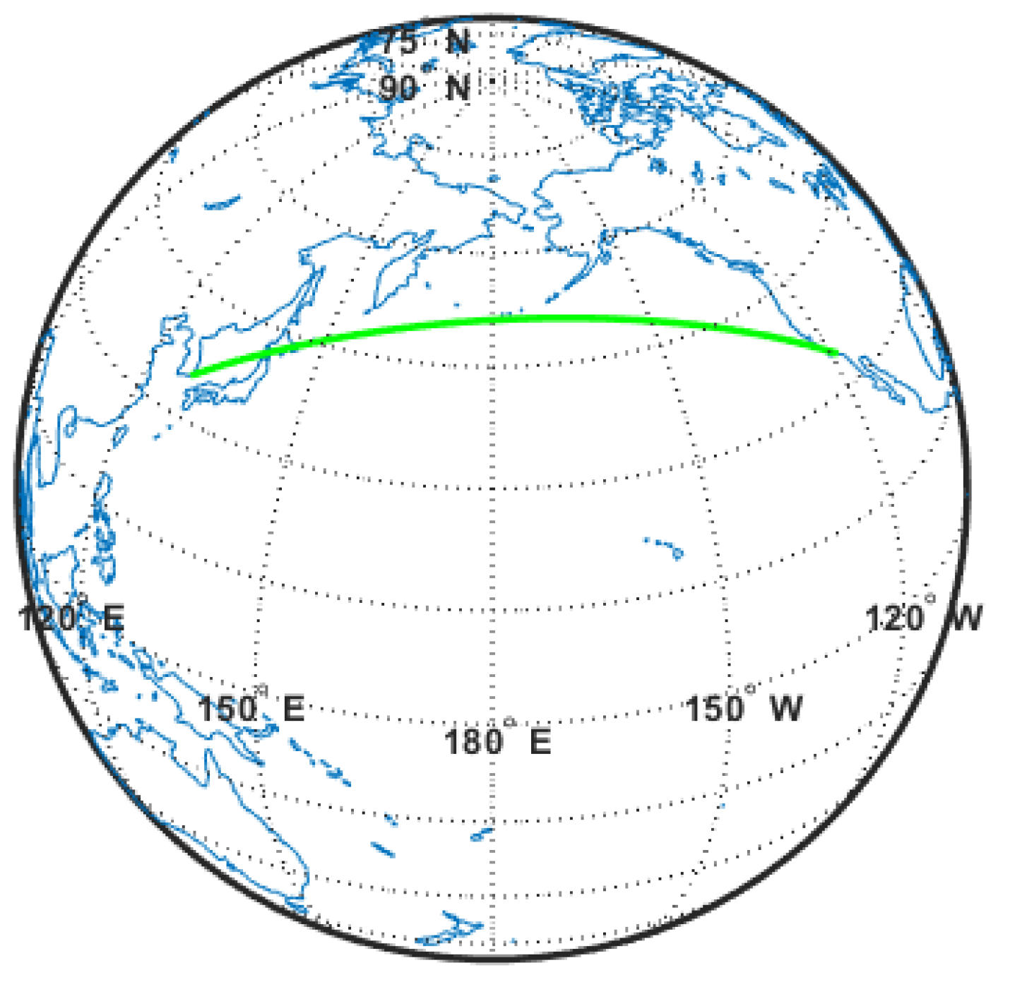
To discuss the speed control method performance for autonomous vessel routing, the real-world voyage cases are employed. The first example is the case of the Pacific voyage. The primary feature of the Pacific voyage is the mild weather as compared to the Atlantic and is also less affected by geographical constraints. Furthermore, it is a highly promising route due to the trade between the United States and Asia in regard to energy products, such as LNG and liquid hydrogen. Therefore, it is a route worthy investigating due to the possibility of application to autonomous vessel.
Generally, the voyage time duration of the Pacific is longer; more than ten days, so it is enough time duration to analyze the superiority of the proposed speed control method. Table 7 and Figure 15 present the great circle route of the Pacific voyage case.
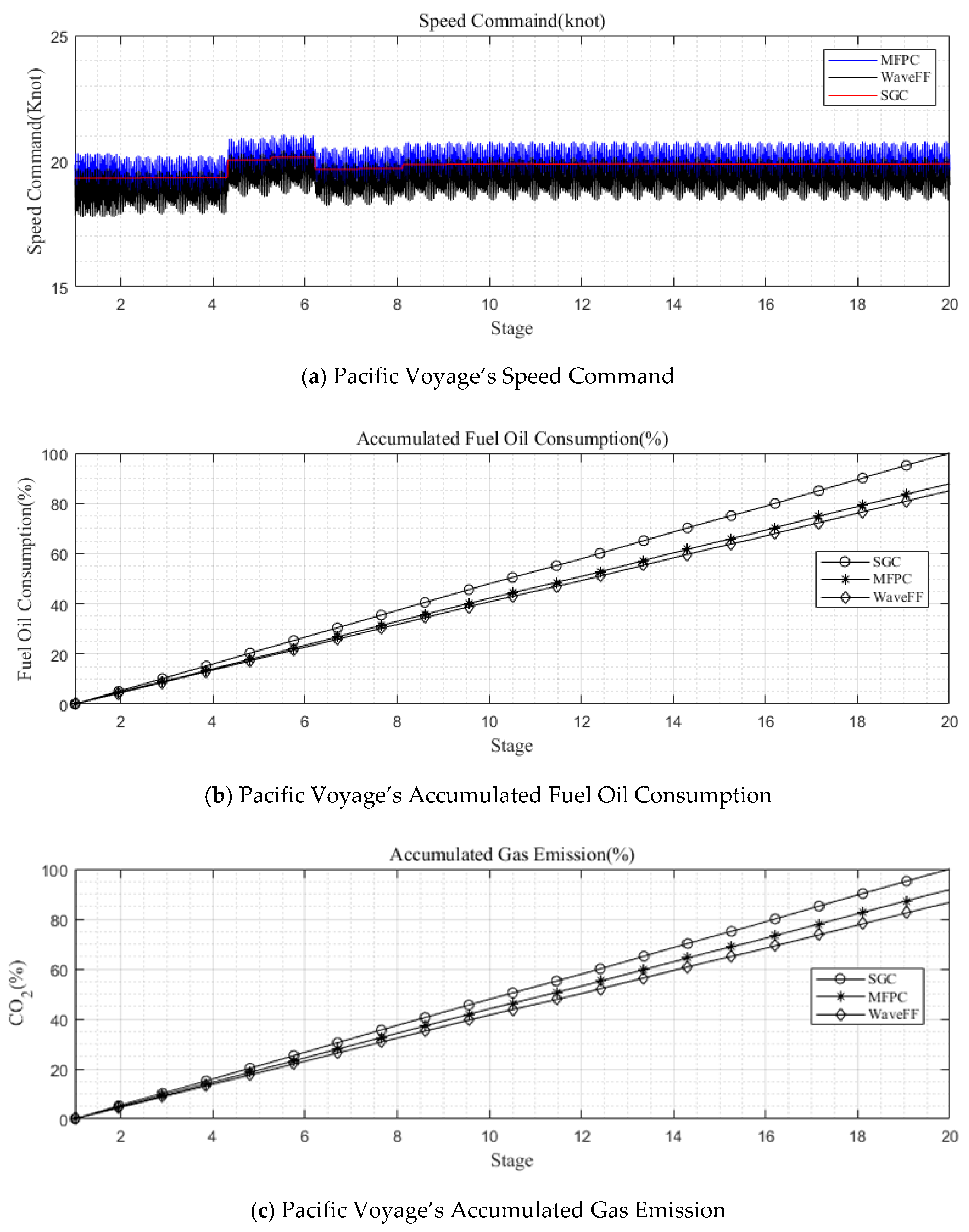
Figure 16 shows the speed command, the accumulative fuel oil consumption, and the gas emission. In Regarding the fuel consumption, the wave feed forward controls the speed well compared to the modified fixed power control. The wave feed forward speed power control is considered superior to the modified fixed power control due to the ability of the wave feed forward to pre-emptively estimate the environmental load compared with the modified fixed power control.
Table 8 shows the voyage planning results due to the speed control methods. The wave feed forward method shows the best performance in terms of fuel oil consumption and gas emission. It saves about 15% of fuel oil consumption and gas emission when a speed governor control is employed. On the other hand, the modified also confirmed its superior performance compared to the conventional speed governor control. It consistently saves about 10% compared to the speed governor control.
4.2. North Atlantic
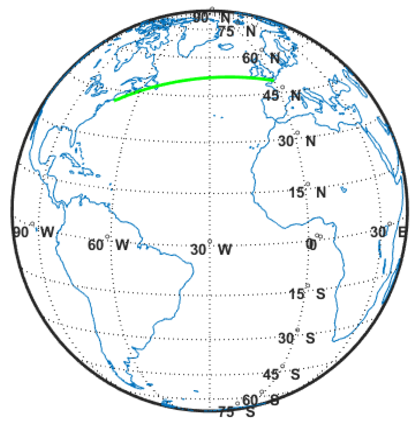
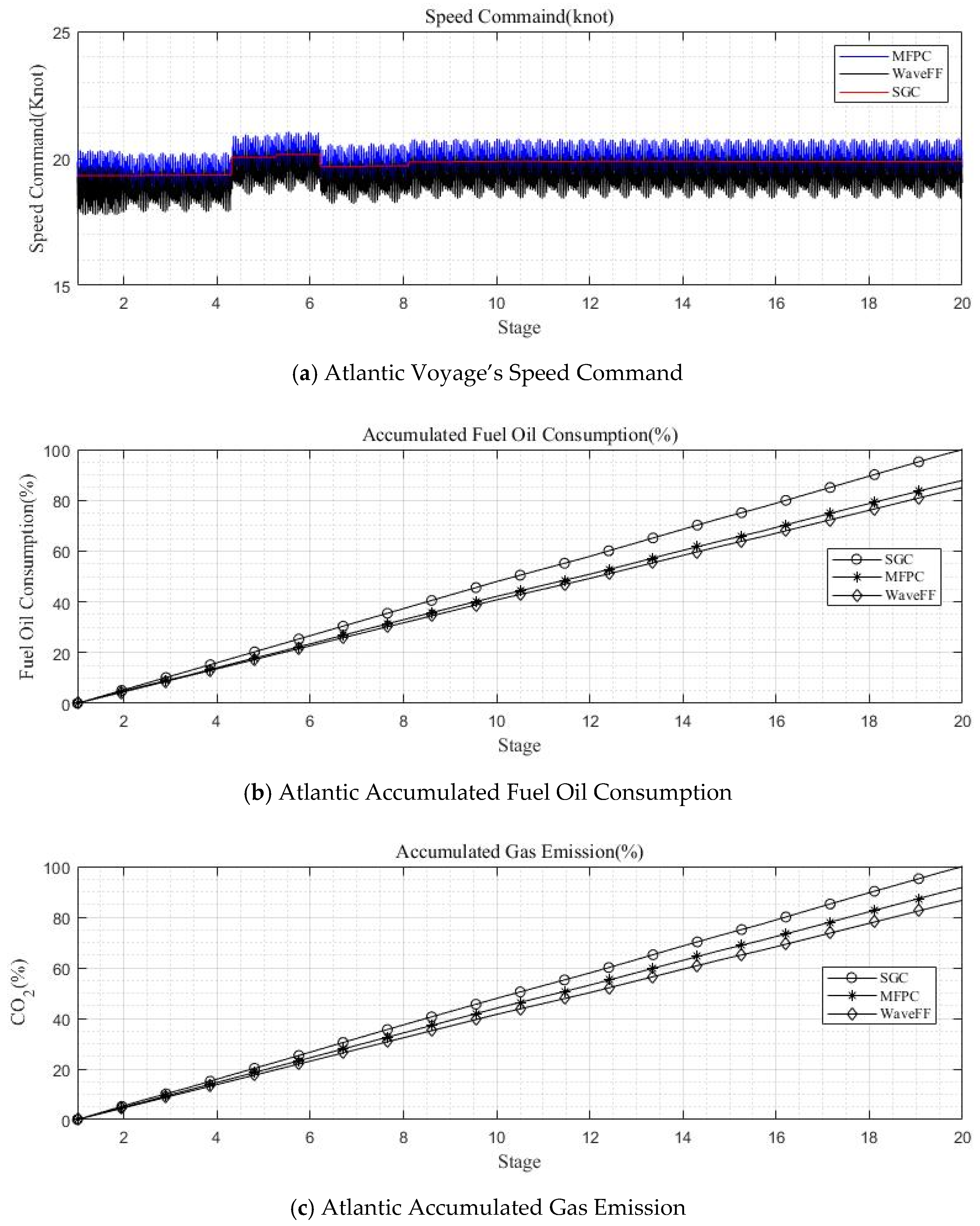
The performance of speed control methods for autonomous vessel routing is presented in the North Atlantic voyage. The case of the North Atlantic Sea is designed to reveal the performance variation of the proposed speed control method according to the adverse weather. Table 9 and Figure 17 present the sample route and the voyage information summary.
Figure 18 and Table 10 shows the speed command, the accumulated fuel oil consumption and gas emission. According to results, the wave feed forward and the modified fixed power control reduce the fuel oil consumption and the gas emission compared to the original speed governor control. As the weather became adverse, the ability of wave feed forward and the modified fixed power control performance to save on fuel oil consumption tended to supersede that of the speed governor control scheme. The reduction in amount of fuel consumption and gas emission become larger compared to the Pacific voyage case. The wave feed forward saves more on fuel oil consumption than in the Pacific case.
5. Conclusions
In this manuscript, two newly developed speed control algorithm for autonomous vessel is proposed. Two speed control algorithms are modified, that is, fixed power control and wave feed forward control method. Both methodologies satisfy the required time of arrival condition and reduce fuel oil consumption and gas emission compared to the existing state of the art speed governor control. The conventional speed governor control is the method that controls the vessel voyage based on the ship speed. It accurately satisfies the required time of arrival. Meanwhile, fuel oil consumption and power of the speed governor control naturally fluctuates due to the environmental disturbances as it tries to maintain its speed in variated environments.
The two proposed methods reduce the fuel oil consumption and the gas emission notably compared to the speed governor control, because the scheme of the proposed method reduces engine acceleration, deceleration, and operates in optimal engine conditions. The proposed methods can save the fuel oil consumption and simultaneously, the engine’s component wear and tear problem. The superiority of the proposed method is also investigated in mild and adverse weather scenarios in real seagoing cases.
Regarding the instantaneous fuel oil consumption and the frequent load variation, they are totally alleviated with the application of the modified fixed power control method and the wave feed forward speed control method. The wave feed forward speed control method shows the best performance and its superiority strengthen in adverse weather conditions. The wave feed forward speed control method shows the best performance in the regards to the fuel oil consumption and gas emission. Situational awareness and local wave height measurement are currently available in the vessel, therefore this technology (proposed method) is also applicable in real voyages.
This paper only considers the marine diesel oil engine operation. There are various engine types, such as dual fuel engine, and a combination of re-liquefaction equipment. This presents a very interesting topic that is worthy to be investigated in the future.
Specifically, fuel gas supply system and partial liquefaction system modeling for ship routing problem will be studied in the future works. There are port berthing optimization studies (Iris et al., [21,22,23]) that consider ship speed as a decision variable and suggest for speeding up. In the future work, port decision making platforms can communicate with ship speed controllers and optimize the overall voyage.
Author Contributions
Conceptualization, S.K.; methodology, S.K.; validation, S.Y. and Y.Y.; formal analysis, S.K.; data curation, S.Y.; writing—original draft preparation, S.K.; writing—review and editing, S.K.; funding acquisition, S.K. All authors have read and agreed to the published version of the manuscript.
Funding
This research was funded by Korea National Information Society Agency, grant project—5G Smart Port Platform Realization.
Institutional Review Board Statement
Not applicable.
Informed Consent Statement
Not applicable.
Data Availability Statement
Not applicable.
Conflicts of Interest
The authors declare no conflict of interest.
Abbreviations
| ATA | Actual Time of Arrival |
| RTA | Required Time of Arrival |
| ETA | Estimated Time of Arrival |
| FOC | Fuel Oil Consumption |
| SFOC | Specific Fuel Oil Consumption |
| QIF | Quadratic Impulse Function |
| QTF | Quadratic Transfer Function |
| SGC | Speed Governor Control |
| FPC | Fixed Power Control |
| MFPC | Modified Fixed Power Speed Control |
| WaveFF | Wave Feed Forward Speed Control |
References
- IMO. Just in Time Arrival Guide—Barriers and Solutions; MEPC 75; IMO: London, UK, 2020. [Google Scholar]
- Wei, S.; Zhou, P. Development of a 3D dynamic programming method for weather routing. TransNav Int. J. Mar. Navig. Saf. Sea Transp. 2012, 6, 79–85. [Google Scholar]
- You, Y.; Choi, J.W.; Lee, D.Y. Development of a framework to estimate the sea margin of an LNGC considering the hydrodynamic characteristics and voyage. Int. J. Nav. Archit. Ocean Eng. 2020, 12, 184–198. [Google Scholar] [CrossRef]
- Kim, S.W. The development of route decision-making method based on tailor-made forecast 2d wave spectra due to the operation profile of the vessel. Ocean Eng. 2020, 197, 106907. [Google Scholar] [CrossRef]
- Kim, S.; Jang, H.; Cha, Y.; Yu, H.; Lee, S.; Yu, D.; Lee, A.; Jin, E. Development of a ship route decision-making algorithm based on a real number grid method. Appl. Ocean Res. 2020, 101, 102230. [Google Scholar] [CrossRef]
- Pratap, S.; Zhang, M.; Shen, C.L.; Huang, G.Q. A multi-objective approach to analyse the effect of fuel consumption on ship routing and scheduling problem. Int. J. Shipp. Transp. Logist. 2019, 11, 161–175. [Google Scholar] [CrossRef]
- Pacheco, M.B.; Soares, C.G. Ship weather routing based on seakeeping performance. In Advancements in Marine Structures; Taylor & Francis Group: London, UK, 2007; pp. 71–78. ISBN 978-0-415-43725-7. [Google Scholar]
- Vettor, R.; Soares, C.G. Development of a ship weather routing system. Ocean Eng. 2016, 123, 1–14. [Google Scholar] [CrossRef]
- De, A.; Choudhary, A.; Tiwari, M.K. Multiobjective Approach for Sustainable Ship Routing and Scheduling with Draft Restrictions. IEEE Trans. Eng. Manag. 2019, 66, 35–51. [Google Scholar] [CrossRef] [Green Version]
- Kwon, Y.J. The Effect of Weather, Particularly Short Sea Waves, on Ship Speed Performance. Ph.D. Thesis, Newcastle University, Newcastle upon Tyne, UK, 1981. [Google Scholar]
- Pennino, S.; Gaglione, S.; Innac, A.; Piscopo, V.; Scamardella, A. Development of a New Ship Adaptive Weather Routing Model Based on Seakeeping Analysis and Optimization. J. Mar. Sci. Eng. 2020, 8, 270. [Google Scholar] [CrossRef]
- Yan, R.; Wang, S.; Du, Y. Development of a two-stage ship fuel consumption prediction and reduction model for a dry bulk ship. Transp. Res. Part E Logist. Transp. Rev. 2020, 138, 101930. [Google Scholar] [CrossRef]
- Du, Y.; Meng, Q.; Wang, S.; Kuang, H. Two-phase optimal solutions for ship speed and trim optimization over a voyage using voyage report data. Transp. Res. Part B Methodol. 2019, 122, 88–114. [Google Scholar] [CrossRef]
- Psaraftis, H.N.; Kontovas, C.A. Speed models for energy-efficient maritime transportation: A taxonomy and survey. Transp. Res. Part C Emerg. Technol. 2013, 26, 331–351. [Google Scholar] [CrossRef]
- Venturini, G.; Iris, Ç.; Kontovas, C.A.; Larsen, A. The multi-port berth allocation problem with speed optimization and emission considerations. Transp. Res. Part D Transp. Environ. 2017, 54, 142–159. [Google Scholar] [CrossRef] [Green Version]
- Zhang, X.; Lam, J.S.L.; Iris, Ç. Cold chain shipping mode choice with environmental and financial perspectives. Transp. Res. Part D Transp. Environ. 2020, 87, 102537. [Google Scholar] [CrossRef]
- Zis, T.P.; Psaraftis, H.N.; Ding, L. Ship weather routing: A taxonomy and survey. Ocean Eng. 2020, 213, 107697. [Google Scholar] [CrossRef]
- Faber, J.; Markowska, A.; Nelissen, D.; Davidson, M.; Eyring, V.; Cionni, I.; Selstad, E.; Kågeson, P.; Lee, D.; Buhaug, Ø.; et al. Technical Support for European Action to Reducing Greenhouse Gas Emissions from International Maritime Transport; CE Delft: Delft, The Netherlands, 2009. [Google Scholar]
- Holtrop, J.; Mennen, G.G.J. An approximate power prediction method. Int. Shipbuild. Prog. 1982, 29, 166–170. [Google Scholar] [CrossRef]
- Kim, S.W. Eco–Friendly Dynamic Positioning Algorithm Development. Ph.D. Thesis, Texas A&M University, College Station, TX, USA, 2016. [Google Scholar]
- Iris, Ç.; Lam, J.S.L. Recoverable robustness in weekly berth and quay crane planning. Transp. Res. Part B Methodol. 2019, 122, 365–389. [Google Scholar] [CrossRef]
- Iris, Ç.; Pacino, D.; Ropke, S. Improved formulations and an adaptive large neighborhood search heuristic for the integrated berth allocation and quay crane assignment problem. Transp. Res. Part E Logist. Transp. Rev. 2017, 105, 123–147. [Google Scholar] [CrossRef]
- Iris, Ç.; Pacino, D.; Ropke, S.; Larsen, A. Integrated berth allocation and quay crane assignment problem: Set partitioning models and computational results. Transp. Res. Part E Logist. Transp. Rev. 2015, 81, 75–97. [Google Scholar] [CrossRef] [Green Version]
Figure 1.
Fuel oil consumption time series due to different speed control methods.

Figure 2.
Fuel Oil Consumption estimation procedure (ISO 15016:2015 and Holtrop–Mennen method).

Figure 3.
Specific fuel oil consumption and gas emission.

Figure 4.
Environmental effects on ship fuel oil consumption modeling.

Figure 5.
Wake and thrust deduction variation.

Figure 6.
Torque and thrust coefficients under waves.

Figure 7.
Conventional state of the art (3DDP) routing algorithm.

Figure 8.
Speed change according to speed control method.

Figure 9.
Fuel oil consumption time history according to speed control methods.

Figure 10.
Schematic diagram of the modified fixed power control.

Figure 11.
Estimated time arrival (modified fixed power control vs. speed governor control).

Figure 12.
Wave feed forward control algorithm.

Figure 13.
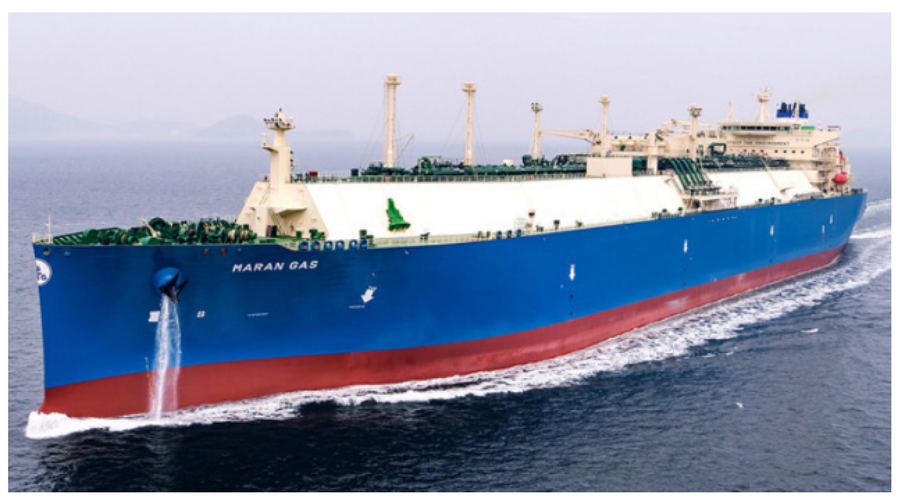
Target vessel—173 K LNG Carrier.

Figure 14.
Speed, fuel oil consumption, and gas emission.

Figure 15.
Pacific route case.

Figure 16.
Pacific voyage planning results.

Figure 17.
The Atlantic Route Case.

Figure 18.
The Atlantic voyage and Pacific voyage planning results.


Table 1.
173 K LNG Carrier engine specification.
| Spec | Type |
|---|---|
| Model | 5G70MEGI |
| Propulsion | Twin |
| Operation Mode | Fuel & Gas |
| Capacity | 12500 kW at MCR |
Table 2.
Principal dimension of 173 K LNG Carrier.
| Item | Unit | Value |
|---|---|---|
| LBP | m | 283.0 |
| Breadth | m | 46.4 |
| Draft | m | 11.5 |
| Propulsion Type | - | Twin |
| Propeller Diameter | m | 8.3 |
Table 3.
Weather condition at voyage stage.
| Stage | Speed Command (K) | Weather |
|---|---|---|
| 1 | 5 | Mild |
| 2 | 7 | Medium |
| 3 | 9 | Adverse |
| 4 | 8 | Adverse |
| 5 | 6 | Mild |
| 6 | 4 | Adverse |
| 7 | 9 | Medium |
| 8 | 10 | Adverse |
| 9 | 6 | Adverse |
| 10 | 4 | Medium |
| 11 | 5 | Mild |
| 12 | 7 | Medium |
| 13 | 9 | Adverse |
| 14 | 8 | adverse |
| 15 | 6 | Mild |
| 16 | 4 | Adverse |
| 17 | 9 | Medium |
| 18 | 10 | Adverse |
| 19 | 6 | Adverse |
| 20 | 4 | Medium |
Table 4.
Example data set for the fuel oil consumption estimation at stage 2.
| Value (Unit) | Value (Unit) | ||
|---|---|---|---|
| Sea State | Medium (-) | t (thrust deduction) | 0.1900 (-) |
| Speed | 7 (Knot) | w (wake) | 0.2500 (-) |
| Rwind | 28 (Kilo Newton) | Powercalm | 273.25 (KW) |
| Rwave | 18 (Kilo Newton) | Powerenvironment | 49.18 (KW) |
| Rcalm | 259 (Kilo Newton) | ηR | 0.973 |
| KT | 0.2827 (-) | ηH | 1.08 |
| KQ | 0.0403 (-) | FOC | 204 ton |
| η0 | 0.4598 (-) | CO2 | 283 ton |
Table 5.
Designed environmental condition (mild, medium, and adverse condition).
| Beaufort | Wind Speed(m/s) | Significant Wave Height (m) |
|---|---|---|
| 3 (Mild) | 4.4 | 0.6 |
| 5 (Medium) | 6.8 | 2.0 |
| 7 (Adverse) | 9.4 | 4.0 |
Table 6.
Voyage results according to speed control methods.
| Speed Governor | Modified Fixed Power | Wave Feedforward | |
|---|---|---|---|
| Fuel Oil Consumption | 100% | 91% | 85% |
Table 7.
The Pacific route conditions.
| Unit | Value | |
|---|---|---|
| Departure Port (Latitude, Longitude) | Degree | 26°12′ N, 127°76′ E |
| Arrival Port (Latitude, Longitude) | Degree | 21°84′ N, 160°24′ W |
| Season | - | Winter |
| Required Time Arrival | Day | 10 |
Table 8.
Pacific case—accumulated FOC and gas emission results.
| Fuel Oil Consumption (%) | Gas Emission (%) | |
|---|---|---|
| Speed Governor | 100.00 | 100.00 |
| Modified Fixed Power | 90.34 | 90.24 |
| Wave Feed Forward | 84.99 | 85.22 |
Table 9.
The Atlantic route conditions.
| Unit | Value | |
|---|---|---|
| Departure Port (Latitude, Longitude) | Degree | 49°49′ N, 0°11′ E |
| Arrival Port (Latitude, Longitude) | Degree | 41°28′ N, 70°10′ W |
| Season | - | Winter |
| Required Time Arrival | Day | 7.5 |
Table 10.
The Atlantic case—accumulated FOC and gas emission results.
| Fuel Oil Consumption (%) | Gas Emission (%) | |
|---|---|---|
| Speed Governor | 100.00 | 100.00 |
| Modified Fixed Power | 87.83 | 91.74 |
| Wave Feed Forward | 84.18 | 85.64 |
Publisher’s Note: MDPI stays neutral with regard to jurisdictional claims in published maps and institutional affiliations. |
© 2021 by the authors. Licensee MDPI, Basel, Switzerland. This article is an open access article distributed under the terms and conditions of the Creative Commons Attribution (CC BY) license (https://creativecommons.org/licenses/by/4.0/).
Share and Cite
MDPI and ACS Style
Kim, S.; Yun, S.; You, Y. Eco-Friendly Speed Control Algorithm Development for Autonomous Vessel Route Planning. J. Mar. Sci. Eng. 2021, 9, 583. https://0-doi-org.brum.beds.ac.uk/10.3390/jmse9060583
AMA Style
Kim S, Yun S, You Y. Eco-Friendly Speed Control Algorithm Development for Autonomous Vessel Route Planning. Journal of Marine Science and Engineering. 2021; 9(6):583. https://0-doi-org.brum.beds.ac.uk/10.3390/jmse9060583
Chicago/Turabian StyleKim, Sewon, Sangwoong Yun, and Youngjun You. 2021. "Eco-Friendly Speed Control Algorithm Development for Autonomous Vessel Route Planning" Journal of Marine Science and Engineering 9, no. 6: 583. https://0-doi-org.brum.beds.ac.uk/10.3390/jmse9060583
Note that from the first issue of 2016, this journal uses article numbers instead of page numbers. See further details here.