Hybrid Scheduling for Multi-Equipment at U-Shape Trafficked Automated Terminal Based on Chaos Particle Swarm Optimization

Abstract

Aimed to improve the efficiency of port operations, Shanghai Zhenhua Heavy Industries Co., Ltd. (ZPMC) proposed a new U-shape trafficked automated terminal. The new U-shape trafficked automated terminal brings a new hybrid scheduling problem. A hybrid scheduling model for yard crane (YC), AGV and ET in the U-shape trafficked automated terminal yard is established to solve the problem. The AGV and ET yard lanes are assumed to be one-way lane. Take the YC, AGV and ET scheduling results (the container transportation sequences) as variables and the minimization of the maximum completion time as the objective function. A scheduling model architecture with hierarchical abstraction of scheduling objects is proposed to refine the problem. The total completion time is solved based on a static and dynamic mixed scheduling strategy. A chaotic particle swarm optimization algorithm with speed control (CCPSO) is proposed, which include a chaotic particle strategy, a particle iterative speed control strategy, and a particle mapping space for hybrid scheduling. The presented model and algorithm were applied to experiments with different numbers of containers and AGVs. The parameters of simulation part refer to Qinzhou Port. The simulation results show that CCPSO can obtain a near-optimal solution in a shorter time and find a better solution when the solution time is sufficient, comparing with the traditional particle swarm optimization algorithm, the adaptive particle swarm optimization algorithm and the random position particle swarm optimization algorithm.

1. Introduction

In the booming global logistics, the container terminals, as important parts of ports, are connected to both land and sea transportation. In the increasingly competitive environment, the requirements for container terminal operations are also getting higher and higher. As shown in Figure 1, in the traditional terminal, the yard’s handover areas are set at the ends of each yard block. External trucks (ETs) and automated guided vehicles’ (AGVs) handover are on the land side and the sea side, respectively, and they cannot enter into the yard. The container is transported from/to the AGV or ET to/from the yard crane at the yard block end. The following situations can easily to happen: (1) YCs are always in the state of carrying containers with heavy loads over long distances; (2) YCs are easy to interfere with each other, and it is difficult to take care of loading and unloading ships; (3) the roads of AGV and ET are not completely separated, which is easy to cause congestion; and (4) when ET enters the handover area of the yard, it needs to reverse parking, which is difficult to operate.

The new U-shape trafficked automated terminal is proposed by Shanghai Zhenhua Heavy Industries Co., Ltd. (ZPMC) [1]. It was applied in the Qinzhou Port of Beibu Gulf Port Co., Ltd. [2]. Figure 2 shows the layout of the new U-shape trafficked automated terminal [3]. It is mainly optimized for the yard. Different from the previous handover mode, the U-shape trafficked automated terminal adopts dual cantilever rail cranes as YCs. There are no handover areas at the ends of the yard. YCs’ handover is with AGVs and ETs on both sides of the block, respectively, avoiding long-distance and heavy-load transporting of containers. The AGV and ET have separate lanes. The AGV and ET come from/to the yard along the U-shaped lanes and hand over containers with YC. After the handover work is completed, ET can leave the port directly. Two adjacent storage yard blocks share AGV or ET lanes, and YC can be directly handed over with AGV and ET at both ends of the cantilever. The U-shape trafficked layout is aimed to avoid the problems of traditional terminal by optimizing the handover mode among YC, AGV and ET: (1) YC adopts a structure with a spreader on both ends, and AGVs and ETs can reach the designated position to hand over with YC, avoiding long-time long-distance, heavy-load container handling of YC; (2) the transportation roads of AGVs and ETs are completely separated, so there is no longer a mixed congestion problem of AGV and ET; and (3) and ET can leave the port directly after its handover is completed, which improves the transportation efficiency of the overall operation.

The scheduling strategy of the traditional terminal yard is no longer applicable to the yard under the new U-shape trafficked layout. In the traditional handover mode, AGV or ET hands over with YC in the handover area at both ends of the yard. In the U-shape trafficked layout, AGV or ET enters the yard for handover with YC. AGV and ET lanes are separated, so there is no interference between AGV and ET, but there is a new path interference occurring in AGVs or ETs. Significant changes take place in the handover mode of YC, AGV and ET. Because YC can hand over separately with AGV and ET at same bay (parallel to the YC cart track), we need to consider the mixed constraint between YC, AGV and ET, not just the route interference problem of ET or AGV. Therefore, the existing scheduling schemes of the traditional terminal yard cannot solve the current new problem, which is more complicated and challenging.

The new U-shape trafficked automated terminal is proposed by ZPMC to improve the efficiency of port operations. The handover mode between YC and AGV or ET has changed, bringing new mixed constraints. A new hybrid scheduling problem has arisen in the new U-shaped trafficked automated terminal, which is more complex and harder. In this study, we propose a static and dynamic mixed scheduling strategy to solve the problem, and we abstract the attributes contained in the scheduling object (such as the task scheduling parameters of YC, AGV and ET; the start time and end time of each task; the total task completion time; and the tasks corresponding to the queue at the yard entrance) to form a module. We connected these modules to build a new model architecture. This architecture makes it more convenient to modify and optimize the hybrid scheduling problem. To improve PSO, a chaos particle swarm optimization with speed control (CCPSO) is proposed. In addition, we propose a mapping space from decision variables to particles to solve the contradiction between algorithm iteration and model solving.

The rest of the paper is organized as follows: Section 2 reviews the relevant literature. Section 3 introduces the multi-equipment scheduling layered model structure and develops the hybrid scheduling problem model. Section 4 provides the details of CCPSO, which includes an improvement of particle mapping space, particle chaos strategy and particle speed control strategy for CCPSO. In Section 5, numerical simulation experiments are carried out to verify the effectiveness of the proposed algorithm, and PSO, APSO and RPPSO are used to compare with CCPSO in different container sizes, AGV numbers. The last section gives the conclusion and future research direction.

2. Literature Review

YC, QC, AGV and ET are all common dispatching machines in container terminals. There has been a lot of research aimed at improving the efficiency of these loading and unloading transportation machines. Iris, C. et al. [4] reviewed some innovative technologies in improving port energy efficiency and pointed out that there is a great potential for ports to achieve further energy efficiency, and researchers have many impactful research opportunities. Most of the scheduling research is aimed at the scheduling of a single equipment. Some researchers have studied the QC scheduling, and they mainly solve the container loading and unloading sequence of the QC [5,6] A large number of researchers have studied the YC scheduling. The non-interference constraint of double YCs and the consideration of multiple environmental variables are the research focus of these problems [7,8,9,10,11,12,13]. For AGV scheduling problem, most researchers focus on finding the optimal vehicle allocation and path planning [14,15].

In general, container transportation tasks require the cooperation of multiple resources (such as cranes and vehicles). Separate scheduling of various equipment resources may lead to suboptimal solutions. If there is no proper and efficient schedule (result of container transportation sequences for equipment), waiting time increases, resulting in lost productivity and increased costs. At present, there are still only a few papers on the study of terminal multi-equipment scheduling, especially when three or more kinds of equipment are involved. Iris, C. et al. [16] researched the ship loading problem with transfer vehicle considered. For AGV and YC scheduling problems, Chen, X. et al. [17] designed a task assignment mode under multiple AGVs and YCs scheduling, in which the YC handover area is at the side of the container yard. The AGV path constraint and YC no-crossings interference are considered. To solve these problems effectively, they drew on some research results in the field of multi-robot task assignment problem (MRTA). Based on the construction of AGV space-time network diagram, they used the Alternating Directional MultiPLication (ADMM) algorithm to make the solution approach to the optimal solution better through linear direction coefficient. In QC and AGV scheduling, Houming, F. et al. [18] considered time- and energy-consumption optimization. The energy consumption objectives include the energy consumption of QC operation and the waiting energy consumption caused by disturbance. Due to the interaction between the two objective functions of energy and time consumption, the near optimal solution could only be achieved in accordance with the actual situation. Iris, C. et al. [19] used a robust method for QC scheduling, considering ship loading problem. At present, researches mainly focus on one or two kinds of terminal equipment dispatching, while researches involving more than three kinds of equipment dispatching are relatively few. He, J. et al. [20] established a solving model by integer programming, in which the energy consumption is taken as objective function. They established the fitness function by classifying the energy consumption of QC, terminal truck (TC) and AGV in different motion states. Then the genetic algorithm and PSO algorithm were used to solve the problem. However, their solving model ignored the AGV, TC path interference constraints and the difference between time-consuming of QC and YC. Moreover, the local optimal problem was not resolved well.

To sum up, the current research on terminal multi-equipment scheduling generally focuses on the scheduling between two kinds of equipment at most, such as AGV and YC, AGV and QC, YC and internal truck (IT), etc. However, the interaction among YC, AGV and ET at the U-shape trafficked automated terminal is much closer than that at traditional automated container terminals. Constraints among three kinds of equipment, such as the path constraint of AGV and ET, and the no-crossing constraint of QC or YC, should be considered. This paper studies the hybrid scheduling for YC, AGV and ET at the U-shape trafficked automated terminal, considering the quantity allocation of AGV and path constraint of AGV and ET. CCPSO which combines both advantages of chaos search and particle swarm optimization is proposed for the hybrid scheduling. The algorithm not only converges quickly, but also can effectively avoid the precocity problem.

3. Mathematical Model

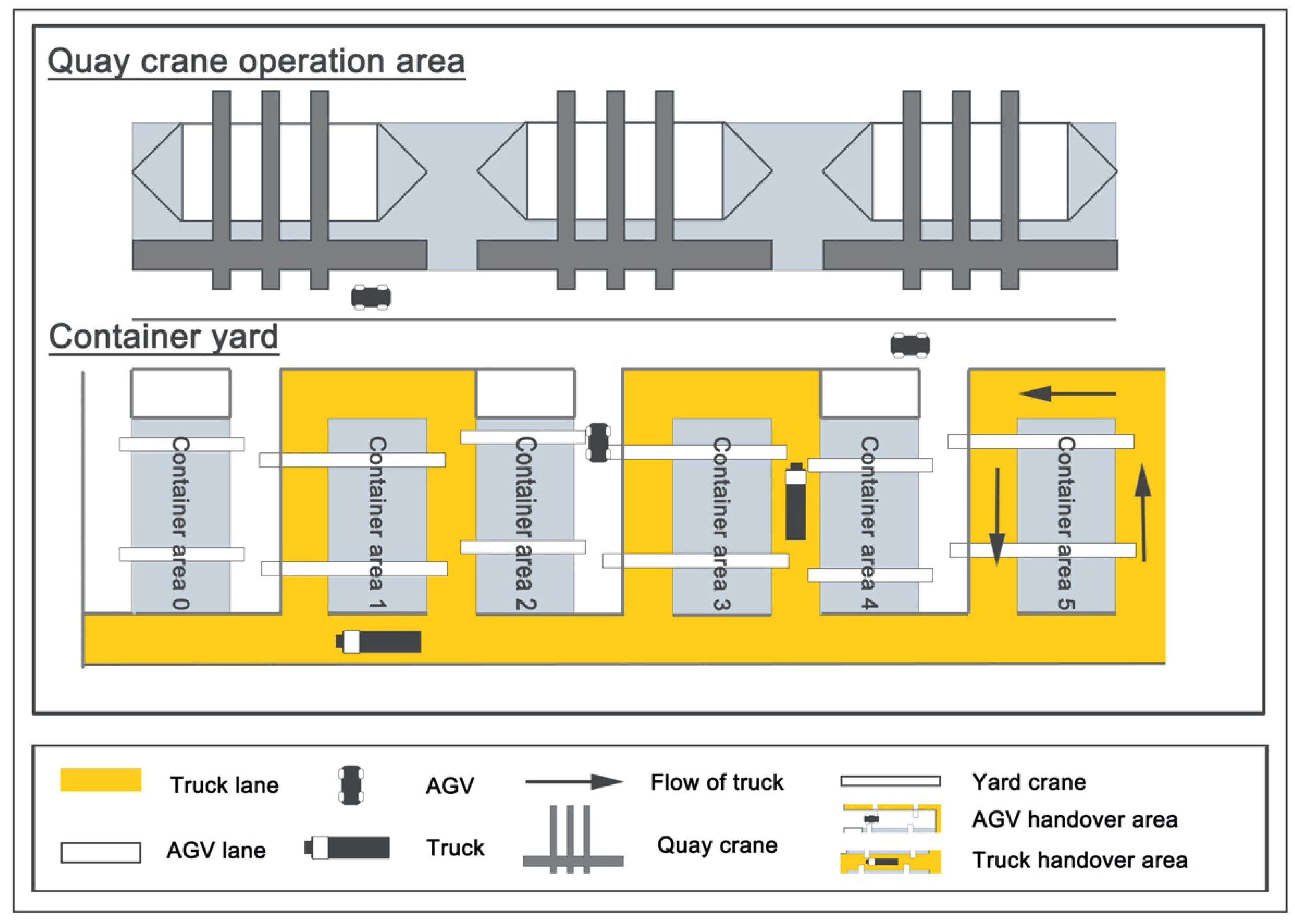
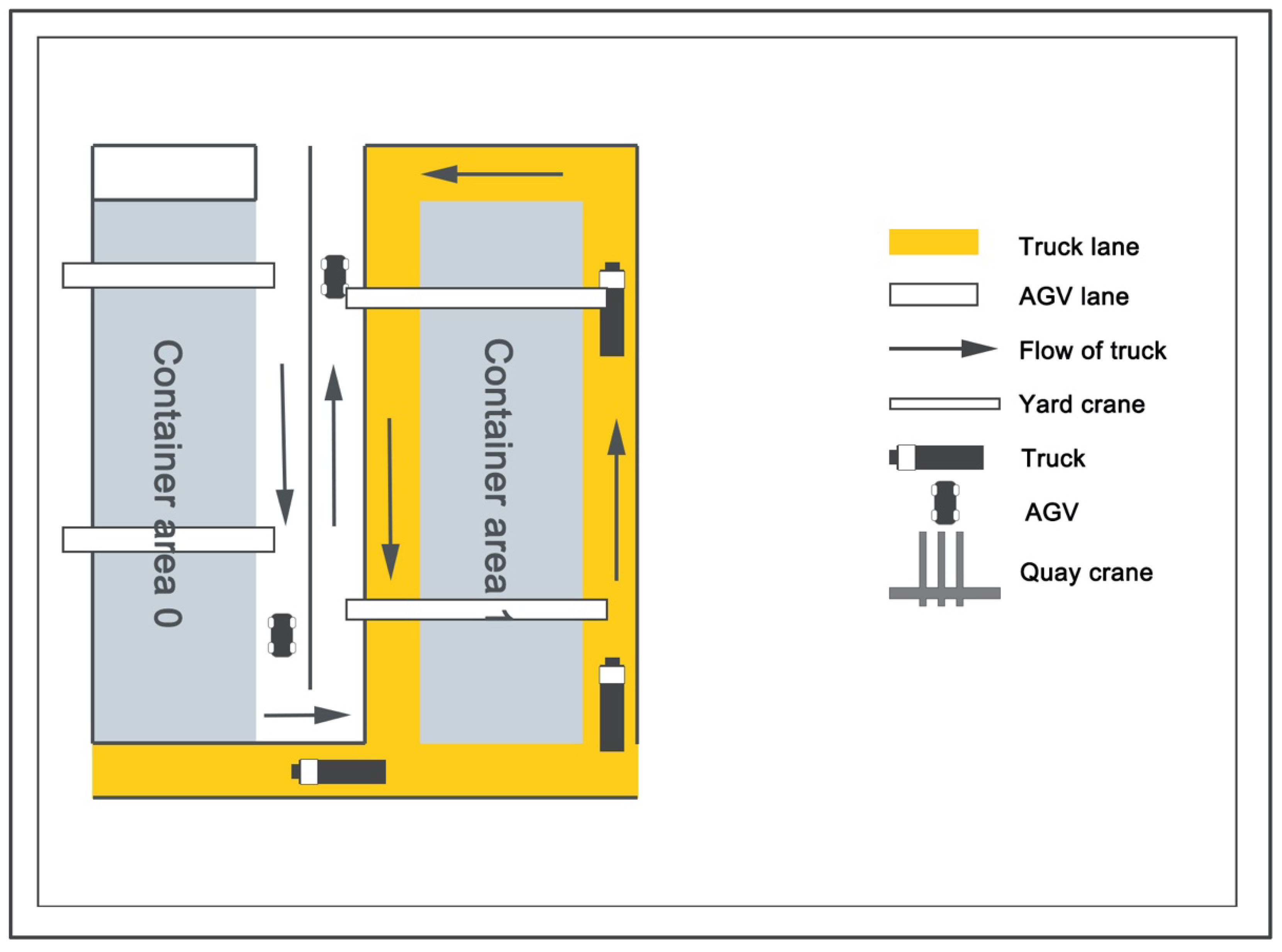
3.1. Problem Description

Figure 3 shows one yard unit of the U-shape trafficked terminal. Each unit contains two blocks. Each block is equipped with 2 YC with spreader on both ends structure, which is responsible for handover with AGV and ET passing by the side of the yard. Before the AGV or ET enters the yard, it needs to queue up and wait in turn at the yard lane entrance. Each AGV or ET enters and exits the yard along the U-shape trafficked route marked in Figure 3. We also have the following assumptions:

• AGV and ET lanes are one-way roads.
• The YC cart running 1 bay consumes one time unit.
• The speed ratio of the YC spreader empty running, the YC spreader full-load running, the YC trolley running, the YC cart empty running and the YC cart full-load running is 1:0.5:0.3:1:0.25 (the speed parameters reference those at Qinzhou Port).
• This study mainly focused on the loading and unloading operations of terminal yard.
• We assume that ET is abundant and one ET is only responsible for one container.

Decision variable can be represented as follows, where two AGVs, two ETs and four YCs are allocated to transport five containers; and 0 and 0* represent the virtual start and end tasks, respectively:

AGV1: 0→1→0*.

AGV2: 0→3→2→0*.

YC1: 0→2→0*.

YC2: 0→3→0*.

YC3: 0→5→4→0*.

YC4: 0→1→0*.

ET1~2: 0→5→4→0*.

3.2. Notations

We introduce the following notations as

Table 1. Parameter notations.

$\mathrm{Parameters}$	Notations
U	YC, AGV and ET, indexed by $u\in \left\{0, 1,2\right\}$.
${\mathrm{YC}}_{i_0}$	Set of YC, indexed by $i_0\in \left\{1,2,3,\dots ,Yc\right\}$.
${\mathrm{ET}}_{i_1}$	Set of ET, indexed by $i_1\in \left\{1,2,3,\dots ,Et\right\}$.
${\mathrm{AGV}}_{i_2}$	Set of AGV, indexed by $i_2\in \left\{1,2,3,\dots ,Agv\right\}$.
${\mathrm{J}}_{i_{\mathrm{u}}}$	Set of equipment task number, indexed by $i_u$, $j\in \left\{{\mathrm{J}}_{i_u}^0, 1, 2, 3, \dots ,{\mathrm{J}}_{i_u}, {\mathrm{J}}_{i_u}^e\right\}$. ${\mathrm{J}}_{i_u}^0$: the virtual initial task; ${\mathrm{J}}_{i_u}^e$: the virtual final task.
$b_n$	Bay where container n should be located.
$r_n$	Row where container n should be located.
${\mathrm{r}}_{agv}$	Handover row of AGV.
${\mathrm{r}}_{et}$	Handover row of ET.
${\mathrm{f}}_n$	The descent distance of the YC spreader when transporting container n.
${\mathrm{f}}_0$	The descent distance of YC spreader during handover.
$d_n$	Task type of container n.
$\mathrm{B}$	Set of yard lane, indexed by $\beta \in \left\{-1, 0,1, \dots ,B\right\}$. −1: entrance of yard lane
${\mathrm{y}}_n$	Block number of container n; 0, block with AGV lane on right hand; 1, block with ET lane on right hand.
sort(x, y)	The function is to adjust the size order of the elements in x to correspond to the size order of the elements in y. For example: x = (0, 1, 2), y = (5, 4, 3), according to the order of the element size in y, x is adjusted to (2, 1, 0).
max(x, y)	The maximum value of x and y.

and

Table 2. Variable notations.

Variables	Notations
F	Maximum completion time.
$y_{ij}$	Container number of YC i, task j.
$a_{ij}$	Container number of AGV i, task j.
$e_{ij}$	Container number of ET i, task j.
$N$	Set of containers, indexed by $n\in \left\{1,2, 3, \dots ,N_{max}\right\}$.
$y{t}_{ij}$	Start time of YC i, task j. $y{t}_{i0}$, start time of the virtual initial task; $y{t}_{ie}$, start time of the virtual final task.
$a{t}_{ij}$	Start time of AGV i, task j. $a{t}_{i0}$, start time of the virtual initial task; $a{t}_{ie}$, start time of the virtual final task.
$e{t}_{ij}$	Start time of ET i, task j. $e{t}_{i0}$, start time of the virtual initial task; $e{t}_{ie}$, start time of the virtual final task.
$S_i^t$	Current handover time of YC i.
$S_i^n$	Current container number of YC i.
$Y_{\beta }^0$	Release time of location $\beta$ on AGV lane. It means that the current AGV lane β at the current moment that AGVs can pass.
$Y_{\beta }^1$	Release time of location$\beta$ on ET lane. It means that ET can pass location$\beta$ on the current ET lane at the current moment that ETs can pass.
$A$	The container number sequence to be performed by the AGVs queued at the entrance of the AGV lane. ${\mathsf{A}}_0$, the first container number; ${\mathsf{A}}_e$, the last container number. 0: a placeholder.
$At$	The arrival time of the AGV in the AGV queue at the entrance of the yard.
${\rm E}$	At the entrance of the ET lane, the container number of the task to be performed by the queued ET.
${\rm E}t$	The arrival time of the ET in the ET queue at the entrance of the yard.

:

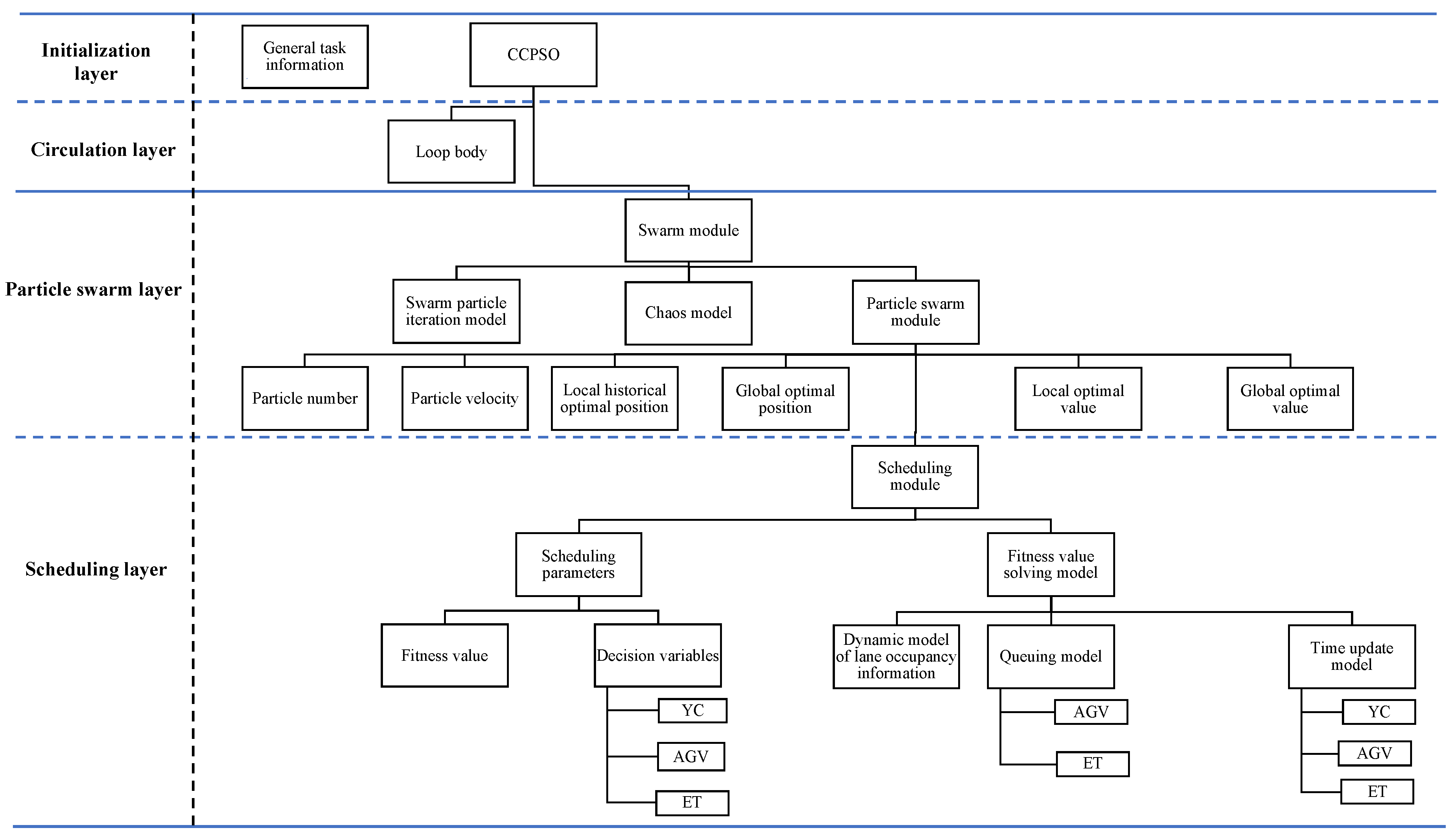
3.3. Layered Architecture

The container terminal scheduling model becomes more and more complex with the increase of container transportation and it is harder to read and understand the scheduling model with constraints increasing. When the considered dynamic variables increase, the scheduling model needs to be re-established, which brings workload. In addition, it brings difficulty in combination of the model and the algorithm. A layered architecture is proposed to optimize the hybrid scheduling model. Each layer of the architecture consists of several modules, and each module consists of several abstract sub-blocks. The abstract sub-blocks become an entity object by setting real value. The logical relationships between modules are determined by the topmost architecture content, so local changes within modules do not affect the whole. The new architecture can capture the key features of problem, and improve the research efficiency.

As shown in Figure 4, the model is firstly divided into four levels: initialization layer, circulation layer, particle layer and scheduling layer. In the initialization layer, the general task information is used to initialize the particle swarm in the loop body. In the circulation layer the loop body contains the algorithm iteration logic. Both the initialize layer and the circulation layer belong to the outer framework of the model. The outer framework is mainly responsible for the initialization of the abstract module, as well as the algorithm cycle for iteration and calculation. The inner architecture includes the particle swarm layer and the scheduling layer. The particle swarm layer includes the algorithm method (particle iteration model and chaos model in Figure 4), and the swarm module is an abstraction of the particle swarm, the abstract particle module can be objectified through this part. The particle swarm parameters generally include the total number of particles, the velocity of each particle, the local historical optimal position, the global optimal position, the global optimal value and the local historical optimal value. In the scheduling layer, scheduling module belongs to the abstraction of the single decision variable of scheduling problem, and it includes the scheduling parameters and fitness value solving model. In this paper, the scheduling parameters include the fitness value and the decision variables (scheduling arrangements of YC, AGV and ET). After the model initialized, the scheduling parameters of the scheduling module become real objects. When the fitness value solving model is called by the outer structure, the dynamic tracking model of the lane occupancy information, the queuing model and the time update model are used to solve the completion time of current decision variables. The solving value is then assigned to the fitness value.

3.4. Model

3.4.1. Objective Function

$$\min F=\max \left(y{t}_{i_{0}e},e{t}_{i_{1}e},a{t}_{i_{2}e}\right)$$

(1)

Objective Function (1) is used to minimize the overall maximum completion time, F, which depends on the final completion time of the transportation equipment (YCs, AGVs and ETs).

3.4.2. Static and Dynamic Mixed Scheduling Strategy

Shyalika et al. [21] mentioned that the scheduling strategies in current research are mainly divided into static scheduling and dynamic scheduling. In static scheduling, the decision variables (task assignment) are assumed to be known in the computation. In dynamic scheduling, the decision variables are unknown in the computation, and many parallel strategies are generated in the computation project until the last task is assigned.

As shown in Figure 5, in the U-shape trafficked terminal, one YC task’s completion time depends on the arrival time of AGV or ET at the handover area. Meanwhile, to satisfy the path interference constraint, there is a waiting time as AGV or ET is waiting until other AGVs or ETs on its path are leaving. Thus, the arrival time of AGV or ET to the handover area is affected by other AGVs or ETs. When arriving at the handover area, AGV or ET waits for YC to complete its handover work. YC, AGV and ET are mutually restrictive when transporting containers in the yard. Therefore, the coupling relationship between YC, AGV and ET in the U-shape trafficked terminal yard is described as a mixed constraint problem. Since the previous static strategy is not able to solve the problem, static strategy is combined with dynamic strategy in this study. This strategy tracks road occupancy information by assuming that the decision variables are known, and it uses a dynamic solution to solve the fitness value, that is, the maximum completion time.

(a) Static Scheduling

The algorithm loop is based on known decision variables. The tasks information including the container number, the task type corresponding to the container, the target location of the container in yard is input to initialize the computation. Each container has a unique numerical number. The corresponding tasks of each container are divided into four types as shown in

Table 3. Task type.

Task Type	Equipment 1	Equipment 2
1	YC	AGV
2	AGV	YC
3	YC	ET
4	ET	YC

below. Type 1 indicates that export containers are transported out of the yard through YC and AGV in turn. Type 2 indicates that containers are transported from AGV to the yard, and then from YC to the target location of the corresponding yard. The transportation modes of types 3 and 4 are similar to types 1 and 2, respectively. For types 1 and 3, YC moves to the target location of the yard to get the container first, and then it waits until AGV or ET arrives at the handover area. The current task is completed after YC finishes the handover. For task type 2 and 4, the YC trolley first moves to the handover row of target bay and then waits for the handover with AGV or ET. Then YC only needs the movement of the trolley and spreader to transport the container to the target location at the current yard location.

AGVs or ETs need to line up at the entrance of the yard first, and enter or leave when there are no other AGVs or ETs on path. The AGV that first hands over with YC at the yard has priority. At the handover area, YC, AGV or ET need to wait until the corresponding handover equipment arrives. The completion time of the current task is impacted by the transportation and handover time of the transportation equipment, and the completion time of the previous task. Thus, there is a coupling relationship between the above problems. In addition to solving the hybrid scheduling problem of YC, AGV and ET, it is necessary to access their status in real time.

(b) Dynamic Scheduling

Since the bay is parallel to the lane at the yard, the bay position can be corresponded to the lane coordinates one to one. Through the occupancy status of each location in yard lanes, the information of AGV or ET entering the yard can be tracked in real time. As shown in

Table 4. Lane tracking.

Lane Coordinates	Release Time (AGV Lane)	Release Time (ET Lane)
−1	0	0
0	2	15
1	10	3
2	5	9
…	…	…

whether AGV or ET can move is decided by the lane occupancy information. If the lane coordinates are released, the location can be passed. When one AGV or ET waits on the lane, the release time of the corresponding coordinate position is renewed.

When the value of decision variable is initialized, the dynamic scheduling starts until the solving the fitness value and update the decision variable to satisfy all the constraints. When the current container is transported by AGV or ET, the dynamic process and the information updated in process are shown in Figure 6. At each iteration of the dynamic scheduling, all YC tasks are traversed one by one. When all the tasks of a YC are performed, the YC is skipped, and the dynamic process stops until all the YC tasks are traversed. As one YC task is traversed, the AGV or ET transporting the same container is lined up at entrance of queue, and the container numbers and arrival times of AGVs or ETs in queue are updated. Then the AGV or ET at the top of the queue enters the yard at the time the entrance lane released. Through the road occupancy information, we can know whether there are other AGVs or ETs on path. Moreover, the road occupancy information is updated once an AGV or ET arrives, waits or leaves. At the handover process, the start time of the YC task may be updated if the AGV or ET arrives at the handover position later than the YC. After the AGV or ET leaves, the designed task pointer for the current YC continues to track the subsequent YC tasks until all YC tasks are completed.

Constraint (2) defines the initialization of $y{t}_{ij}$ where AGV and ET interference is not taken into account. In the following dynamic scheduling, $y{t}_{ij}$ is updated continuously, until all the constraints are met.

Constraint (3) defines the update of the container number of the current YC task $S_i^n$. When all of the YC tasks are traversed, $S_i^n$ is set to 0 as a placeholder. Constraint (4) defines the update of $S_i^t$ when YC i arrives at the handover area.

$$y{t}_{ij+1}=\{\begin{array}{c}y{t}_{ij+1}+\max \left(\frac{\left|b_{y_{ij}}-b_{y_{ij-1}}\right|}{0.25}+\frac{\left|r_{agv}-r_{y_{ij-1}}\right|}{0.3}\right)+\frac{\left|r_{agv}-r_{y_{ij}}\right|}{0.3}+3(f_{y_{ij}}+f_0),d_{y_{ij}}\in \left\{1,2\right\}\\ y{t}_{ij+1}+\max \left(\frac{\left|b_{y_{ij}}-b_{y_{ij-1}}\right|}{0.25}+\frac{\left|r_{y_{ij}}-r_{y_{ij-1}}\right|}{0.3}\right)+\frac{\left|r_{et}-r_{y_{ij}}\right|}{0.3}+3(f_{y_{ij}}+f_0),d_{y_{ij}}\in \left\{3,4\right\}\end{array}$$

(2)

$$S_i^n=\{\begin{array}{c}0, j\ge {\mathrm{J}}_{i_0}\\ y_{ij}, other\end{array}$$

(3)

$$S_i^t=\{\begin{array}{c}y{t}_{ij}+\max \left(\frac{\left|b_{y_{ij}}-b_{y_{ij-1}}\right|}{0.25}+\frac{\left|r_{y_{ij}}-r_{y_{ij-1}}\right|}{0.3}\right)+3f_{y_{ij}}+\frac{\left|r_{agv}-r_{y_{ij}}\right|}{0.3},d_{y_{ij}}=1\\ y{t}_{ij}+\max \left(\frac{\left|b_{y_{ij}}-b_{y_{ij-1}}\right|}{0.25}+\frac{\left|r_{y_{ij}}-r_{y_{ij-1}}\right|}{0.3}\right)+3f_{y_{ij}}+\frac{\left|r_{et}-r_{y_{ij}}\right|}{0.3},d_{y_{ij}}=3\\ y{t}_{ij}+\max \left(\frac{\left|b_{y_{ij}}-b_{y_{ij-1}}\right|}{0.25}+\frac{\left|r_{agv}-r_{y_{ij-1}}\right|}{0.3}\right),d_{y_{ij}}=2\\ y{t}_{ij}+\max \left(\frac{\left|b_{y_{ij}}-b_{y_{ij-1}}\right|}{0.25}+\frac{\left|r_{et}-r_{y_{ij-1}}\right|}{0.3}\right),d_{y_{ij}}=4\end{array}$$

(4)

$$\mathrm{A}=\mathrm{A}+\left\{y_{i_0^{\prime }{j}_0^{\prime }}\right\}$$

(5)

$$\mathsf{A}t=\mathsf{A}t+\left\{a{t}_{ij}\right\},\forall a_{ij}=y_{i_0^{\prime }{j}_0^{\prime }}$$

(6)

$$a=sort\left(\mathrm{a},\max \left(At,S_i^t\right)\right),\forall i\in \left\{1,2,3,\dots ,Yc\right\}$$

(7)

$$i_1=i,j_1^{\prime }=j,\forall a_{ij}={\mathsf{A}}_0$$

(8)

$$j_1=j,\forall a{t}_{i_{1}j-1}\ne 0,a{t}_{i_{1}j}=0$$

(9)

$$a_{i_{1}j}=\{\begin{array}{c}{\mathsf{A}}_0, j=j_1\\ a_{i_{1}j-1}, j\in \left(j_1,j_1^{\prime }\right]\\ a_{i_{1}j}, j\in \left(j_1^{\prime },{\mathrm{J}}_{i_1}\right]\end{array}$$

(10)

$$t_{enter}=\max \left(a{t}_{i_1{j}_1},Y_{-1}^0+0.1\right)$$

(11)

$$t_{handover}=\max \left(t_{enter},Y_{\beta }^0+∆{\mathrm{t}}_0\right),\forall \beta \le b_{{\mathsf{A}}_0}\ast \left(y_{{\mathsf{A}}_0}+1\right)$$

(12)

$$Y_{-1}^0=t_{handover}$$

(13)

$$i_0=i,j_0=j,\forall y_{ij}={\mathsf{A}}_0$$

(14)

$$y{t}_{i_0{j}_0}=y{t}_{i_0{j}_0}+t_{handover}-S_{i_0}^t,\forall t_{handover}>S_{i_0}^t$$

(15)

$$t_{wait}=\max \left(t_{handover},S_{i_0}^t\right)+3f_0$$

(16)

$$t_{leave}=\max \left(t_{wait},Y_{\beta }^0+∆{\mathrm{t}}_0\right),\forall \beta \le B$$

(17)

$$Y_{\beta }^0=t_{leave},\forall \beta =b_{{\mathsf{A}}_0}\ast \left(y_{{\mathsf{A}}_0}+1\right)$$

(18)

$$a{t}_{i_1{j}_1+1}=t_{leave}+∆{\mathrm{t}}_1$$

(19)

$$\mathsf{A}=\mathsf{A}-\left\{{\mathsf{A}}_0\right\}$$

(20)

Constraints (5) to (20) define the dynamic update process when $y_{{i^{\prime }}_0{j^{\prime }}_0}$ is transported by AGV. When there is an YC for a new task and this task’s container is also transported by the AGV, the task information of AGV queue at entrance is updated. The new arrival is put at the end of the AGV queue. Constraints (5) and (6) define the update of AGV queue’s information at the yard entrance, which includes A and At. Constraints (7) define the queuing priority. The earlier the AGV and its corresponding YC arrive at the entrance and handover area, the higher priority the AGV has. Each time an AGV enters the queue, the AGV queue at the yard entrance is rearranged according to the above priority. Constraint (8) and (9) defines AGV number $i_1$ and task number $j_1$ of the top AGV at the current AGV queue. Since the AGV container task sequence changes after the re-queuing, the AGV scheduling order also needs to be updated according to constraint (10). Constraints (11) to (19) define the update of $a{t}_{i_{1}j}$, $y{t}_{ij}$ and the release time of the position $Y_{\beta }^0$ on handover lane. Constraints (11), (12) and (17) define the entry, handover and departure time of AGV with task $a_{i_1{j}_1}$, considering that the path interference (AGV or ET can move when there is no AGV or ET on its path). Constraint (11) defines the entry time of AGV $i_1$, which is decided by the release time of AGV lane’ entrance and the arrival time of AGV $i_1$. Constraint (12) defines the time AGV $i_1$ arriving at the handover area, $∆{\mathrm{t}}_0$ is a constant coefficient used for collision avoidance. Constraint (13) defines the update of release time of AGV lane’s entrance. Constraint (14) defines the YC number $i_0$ and task number $j_0$ responsible for the transportation. As mentioned above,$y{t}_{i_{0}j}$ is initialized first, as AGV and ET constraints are not taken into account. Constraint (15) defines the update of $y{t}_{i_{0}j}$ when YC $i_0$ need to wait AGV $i_1$ at the handover area. Constraint (16) defines the waiting time of AGV $i_1$ at the handover area. Constraint (17) defines the departure time of AGV $i_1$. Constraint (18) defines the update of the lane release time after AGV $i_1$ leaves. Constraint (19) defines the update of the completion time of AGV $i_1$ task $j_1$ (the completion time of the task is defined as the start time of the next task). $∆{\mathrm{t}}_1$ is a constant coefficient which describes how long the AGV spends until it reaches the entrance of the yard next time. Constraint (20) defines the update of the AGV queue at the entrance.

$${\rm E}={\rm E}+\left\{y_{i_0^{\prime }{j}_0^{\prime }}\right\}$$

(21)

$${\rm E}t={\rm E}t+\left\{e{t}_{ij}\right\},\forall e_{ij}=y_{i_0^{\prime }{j}_0^{\prime }}$$

(22)

$$e=sort\left(e,\max \left(Et,S_i^t\right)\right),i\in \left\{1,2,3,\dots ,Yc\right\}$$

(23)

$$i_2=i,j_2^{\prime }=j,\forall e_{ij}={{\rm E}}_0$$

(24)

$$j_2=j,\forall e{t}_{i_{2}j-1}\ne 0,e{t}_{i_{2}j}=0$$

(25)

$$e_{i_{2}j}=\{\begin{array}{c}{{\rm E}}_0, j=j_2\\ e_{i_{2}j-1}, j\in \left(j_2,j_2^{\prime }\right]\\ e_{i_{2}j}, j\in \left(j_2^{\prime },{\mathrm{J}}_{i_2}\right]\end{array}$$

(26)

$$t_{enter}=\max \left(e{t}_{i_2{j}_2},Y_{-1}^1+0.1\right)$$

(27)

$$t_{handover}=\max \left(t_{enter},Y_{\beta }^1+∆{\mathrm{t}}_0\right),\forall \beta \le b_{{{\rm E}}_0}$$

(28)

$$Y_{-1}^1=t_{handover}$$

(29)

$$i_0=i,j_0=j,\forall y_{ij}={\mathsf{{\rm E}}}_0$$

(30)

$$y{t}_{i_0{j}_0}=y{t}_{i_0{j}_0}+t_{handover}-S_{i_0}^t,\forall t_{handover}>S_{i_0}^t$$

(31)

$$t_{wait}=\max \left(t_{handover},S_{i_0}^t\right)+3f_0$$

(32)

$$t_{leave}=\max \left(t_{wait},Y_{\beta }^1+∆{\mathrm{t}}_0\right),\forall \beta \le B$$

(33)

$$Y_{\beta }^1=t_{leave},\forall \beta =b_{{{\rm E}}_0}$$

(34)

$$e{t}_{i_2{j}_2+1}=t_{leave}+∆{\mathrm{t}}_1$$

(35)

$$E=E-\left\{{{\rm E}}_0\right\}$$

(36)

Constraints (21) to (36) define the dynamic update process when container is transported by ET. The update process of ET is similar to that of AGV. It should be noted that ET can only hand over with YC in the first half of the U-shape trafficked lane, while AGV can hand over with the YCs of different blocks in the first half and the second half of the AGV lane.

4. The Algorithm

4.1. Particle Mapping Space

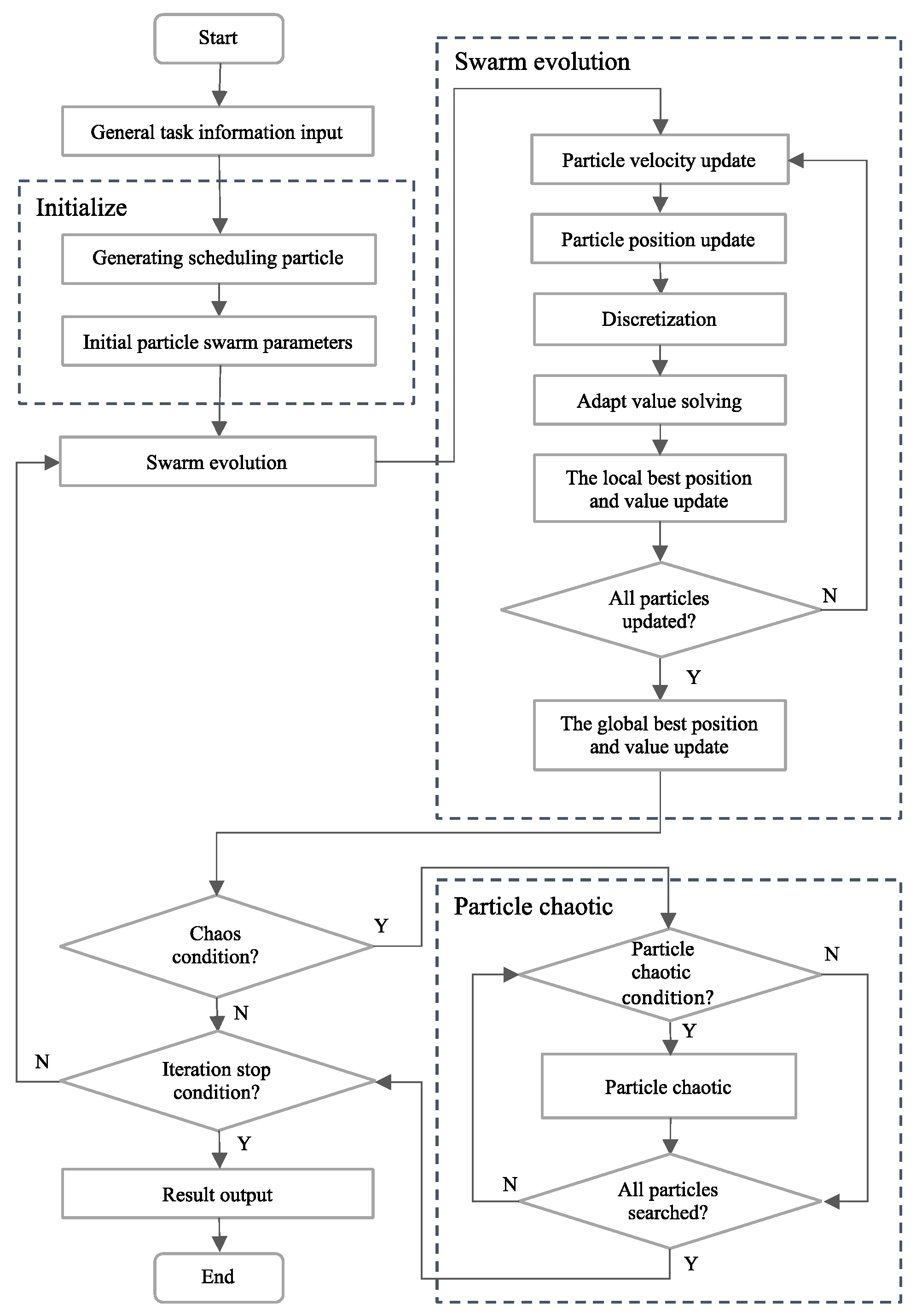
Scheduling decision variables are generally represented by integers, but integer particles are not conducive to iteration. Therefore, continuous mapping of decision particles is required in algorithm iteration. Most researchers simply map the elements in decision variables directly to the 0 to 1 space [22,23]. On this basis, some researchers used the roulette method to improve [20]. In the iteration, the decision variables in the form of integer are used in the fitness function of the scheduling problem. Therefore, the particles in the real number domain need to be discretized. To ensure the consistency between the decision variables and the particles, researchers often arrange the order of the size of the elements in the particles according to a fixed order of decision values. However, this brings some problems. Figure 7 shows a group of two-element particles. The particle distribution space is divided by the dotted line x0 = x1. It can be seen that x0 < x1 below the dotted line, while x0 > x1 the elements above the dotted line. When the particles are mapped to decision variables in the order of element size, the upper and lower parts of the dashed line are only mapped to two decision variable values. After algorithm iteration, the value of the decision variable corresponding to the particle is only related to the arrangement of the element size in the particle. That is, the value of the decision variable is only related to the angle between the particle and each axis, and has nothing to do with the actual element value of the particle. When the above particles are used for iteration, the distribution of the optimal solution diverges along the line. When the dimensionality of the decision variable increases, this feature interferes with the iterative direction correction in the iteration process and affect the final solution result. Therefore, this paper uses the angle between the decision variable and each axis as the particle to avoid the above problems. The relevant formulas are (37) and (38).

$${\theta }_i=arcos\frac{X·E_i}{\left|X\right|}$$

(37)

$$X=sort\left(\mathrm{M},cos \theta \right)$$

(38)

where X is the decision variable, $\theta$ is the algorithm particle, ${\theta }_i$ is the i-th dimension element of $\theta$, $E$ is the identity matrix with the same dimension as X, $\mathrm{M}$ is the reference decision value and $E_i$ is the i-dimensional vector of E.

Equation (37) represents the i-th dimension element of the particle mapped to the decision variable. The element of θ is composed of the angle between X and its axes (the number of axes is determined by the number of elements contained in X). Equation (38) represents the process of mapping continuous particles into discrete decision variables. According to the order of the cos θ and the decision value M referenced by the size ordering, the decision variable X corresponding to the particle θ is finally obtained.

An example is shown in

Table 5. The angle mapping.

M	X	$\mathit{\theta }$ (Radian)	$\mathit{c}\mathit{o}\mathit{s} \mathit{\theta }$
1	13	1.058	0.491
9	9	1.224	0.340
13	14	0.923	0.603
14	16	1.015	0.528
16	1	1.533	0.038

M is the initial mapping rule, and X is the decision particle. It can be seen that X contains 5 elements, and elements in particle θ are angles between X and [1, 0, 0, 0, 0], [0, 1, 0, 0, 0], [0, 0, 1, 0, 0], [0, 0, 0, 1, 0], [0, 0, 0, 0, 1]. The index number of cos θ sorted from small to large becomes [5, 2, 1, 4, 3]. According to the reference decision value M, X becomes [13, 9, 14, 16, 1] after mapping.

4.2. Algorithm

4.2.1. Particle Velocity Control Strategy

Traditional particle swarm optimization (PSO) simulates the social behavior of birds in the foraging process. In each iteration, the current iteration velocity of each particle is determined by local optimal position and global optimal position. The velocity and position are normally updated by the following formulae:

$$v_{i+1}=\omega v_i+c_1{r}_1\left(pbes{t}_i-p_i\right)+c_2{r}_2\left(gbest-p_i\right)$$

(39)

$$p_{i+1}=p_i+v_{i+1}$$

(40)

where $v_i$ is the velocity of particle at i-th iteration; $\omega$ is the inertia weight; $c_1$ is the cognitive coefficient; $c_2$ is the social coefficient; $r_1$ and $r_2$ random numbers in (0, 1), regenerated in each iteration; $pbes{t}_i$ is the local best position of particle; and$gbest$ is the global best position of swarm,$p_i$ is the position of particle.

In CCPSO, a sort of chaos optimization is added to prevent particles from falling into local optimum, and the search performance of the algorithm is improved by increasing the iterative convergence velocity of particles. The velocity is controlled according to (41)–(43):

$$\alpha =\frac{v_{i+1}·\left(p-gbest\right)}{\left|v_{i+1}\right|\ast \left|p-gbest\right|}$$

(41)

$$v_{i+1}{}^{\prime }=\frac{v_{i+1}}{\left|v_{i+1}\right|}\ast \left|p-gbest\right|\ast \alpha$$

(42)

$$p_{i+1}{}^{\prime }=p+v_{i+1}{}^{\prime }$$

(43)

where $v_{i+1}{}^{\prime }$ is the updated velocity of $v_{i+1}$ after velocity control, $\alpha$ is the angle between $v_{i+1}$ and the direction from $p_{i+1}$ to $gbest$ and $p_{i+1}{}^{\prime }$ is the updated local best position of $p_{i+1}$ after velocity control.

At the i-th iteration, particle velocity and position are updated by (48) and (49), and then the final particle position and velocity are updated by the velocity control strategy.

The iteration procedure of CCPSO is as follows:

• Begin.
• Step 1. Input particle position and velocity.
• Step 2. Update the particle position and velocity based on (39) and (40).
• Step 3. The position of particles is limited in (0, $\frac{\pi }{2}$).
• Step 4. If $\alpha >0$, turn to Step 5; otherwise, turn to Step 6; $\alpha$ is calculated based on (41).
• Step 5. Update particle position and velocity based on (42) and (43).
• Step 6. Call fitness solving module.
• Step 7. Update the local best and the global best.
• Step 8. Turn to Step 1 until all the particles are traversed.
• End.

4.2.2. Particle Chaos Method

Chaos is a general nonlinear phenomenon; its behavior is complex and similar to random, but it has exquisite internal laws. Because of the ergodicity of chaos, the optimal search using chaotic variables is more advantageous than the random search with blind disorder, and it can avoid the algorithm falling into local optimum. The chaotic mapping method is one of the core contents of chaos search. There are many researches on one-dimensional or two-dimensional chaotic mapping [24,25,26,27].These studies mainly aimed at improving the ergodicity of particles in chaotic mapping space and other related features. The studies about chaotic mapping for higher dimensional space are few in number. In general scheduling problems, multiple tasks and scheduling objects are involved, so applying chaotic search methods to scheduling problems requires reconsideration of the applicable chaotic strategies.

Equation (44) is a commonly used one-dimensional chaotic mapping method. This mapping space is simple to use, and the mapped particles have good randomness and convenience.

$$map\left(x\right)=4x\left(1-x\right),x\in \left(0,1\right)$$

(44)

where $map\left(x\right)$ is chaotic mapping function, and x is the input value.

The particle chaos procedure is as follows:

• Begin.
• Step 1. Input particle position and velocity.
• Step 2. Set $p_c$ (the probability of chaos), and generate a random number x in (0, 1). If x <$p_c$, turn to Step 3; otherwise, turn to Step 4.
• Step 3. Chaos starts from the second element of the particle, and the mapping value is calculated based on the following formula:

  $$P_{ijk}=\min \left(\frac{P_{ijk-1}}{0.5\pi }+0.01,0.9\right)$$

  (45)

  where $P_{ijk}$: The position of the k-th element of the j-th dimension in the i-th particle.
• Step 4. Turn to Step 1 until all the particles are traversed.
• End.

4.2.3. The Algorithm Steps

CCPSO is used to solve the hybrid scheduling for multi-equipment at the U-shape trafficked automated terminal. As mentioned in Section 3, in the hierarchical architecture model, the loop body, the algorithm module and the scheduling module are independent as a whole, and the changes in one module do not affect other parts. Figure 8 shows the loop body (the flowchart of CCPSO) of the hierarchical architecture model in this paper. The whole process is divided into three parts: particle initialization, particle swarm iteration and particle chaos. The input general task information contains the task type and the container locations in the yard. The container location information includes yard, bay and row, which represent the number of the yard block, bay and row locations. Since the hybrid scheduling in this paper involves three kinds of scheduling machines, there are three subgroups in particle swarm.

The iteration procedure of CCPSO for hybrid scheduling optimization of YC, AGV and ET at the U-shape trafficked automatic terminal is as follows:

• Begin.
• Step 1. Input the general tasks information.
• Step 2. Initialize scheduling decision variable YC, AGV and ET.
• Step 3. Initialize particle swarm parameters.
• Step 4. Call the particle swarm iteration module and input the particle swarm.
• Step 5. Call the particle chaos module and input the particle swarm.
• Step 6. Turn to Step 1 until the iteration or the computation time reaches the limit value.
• End.

Figure 9 shows the overall cycle flow of the circulation layer and how each layer relates to the others. Figure 9 summarizes the basic layers of the scheduling problem. They are interconnected through the loop body given by the circulation layer and do not affect each other. This makes the layered structure of this article applicable to different scheduling problems. For example, in other scheduling research, more scheduling equipment needs to be considered, and then it is necessary to build a problem model from scratch and perform algorithm design. The new structure reduces the workload. Under the new structure, only the scheduling module of the scheduling layer needs to be designed at this time.

Section “Dynamic scheduling” has explained the use of dynamic idea to solve the fitness value and container transportation sequence of each equipment. The static solution strategy used in the existing literature cannot be applied to the mixed constraint in the hybrid scheduling problem with multiple equipment types, because, under this type of constraint, the equipment transportation is affected by same type of equipment and different types of equipment. Solving the status of each equipment at each moment is time-consuming and inefficient. When the transportation equipment is doing the task, it is not necessary to pay attention to the status of other equipment at each moment; only when YC, AGV or ET arrives at the designated handover location, it needs to access whether the docking equipment is in place. When the AGV or ET is ready to move, it needs to access whether other equipment is on its current lane to prevent collisions.

The interaction of dynamic information flow was explained in Section “Dynamic scheduling”, and Figure 10 shows the solution process for fitness value and equipment task scheduling sequence based on the dynamic scheduling strategy. For a static scheduling result (YC, AGV and ET container transportation sequence), set YC task pointers for all YCs to traverse. For the task pointed by each YC pointer, the corresponding AGV or ET is queued at the yard block entrance. The sooner the YC arrives at the designated bay, the sooner the AGV or ET arrives at the entrance, and the earlier the container is transported; the AGV or ET transporting the container is closer to the forefront of the queue. Next, the container at the front of the queue is processed. As shown in Figure 10, the AGV or ET acts by accessing the yard block lane occupation information (waiting to reach the target location). The yard block lane is divided according to the bay position, and the lane occupation information records the latest release time of each lane position, after the release time the lane position can be occupied. When the task pointer traverses all tasks, the solving process ends and outputs the scheduling result, which includes the YC, AGV and ET container transportation sequences; each YC, AGV and ET container task’s completion time; and total completion time (fitness value).

5. Validation and Result Analysis

5.1. Parameter Settings

Here, two blocks are considered in the U-shape trafficked automated terminal. The size of each yard is set as bay ∈ [0, 7], row ∈ [0, 5] and fall ∈ [0, 5] (the yard parameters refers to the Qinzhou Port). Two YCs, four AGVs and enough ETs are arranged for each block. In CCPSO, the particle swarm size is 20; the inertia weight ω is 0.729; the cognitive and social coefficients, $c_1$ and $c_2$, are both 1.494$; r_1$ and $r_2$ are random numbers in (0, 1); and the chaos probability, $p_c$, is 30%.

The computer equipped with 2.3 GHz quad-core Intel Core i5, 8 GB 2133 MHz LPDDR3 and Python 3.8 was used in following scheduling experiments.

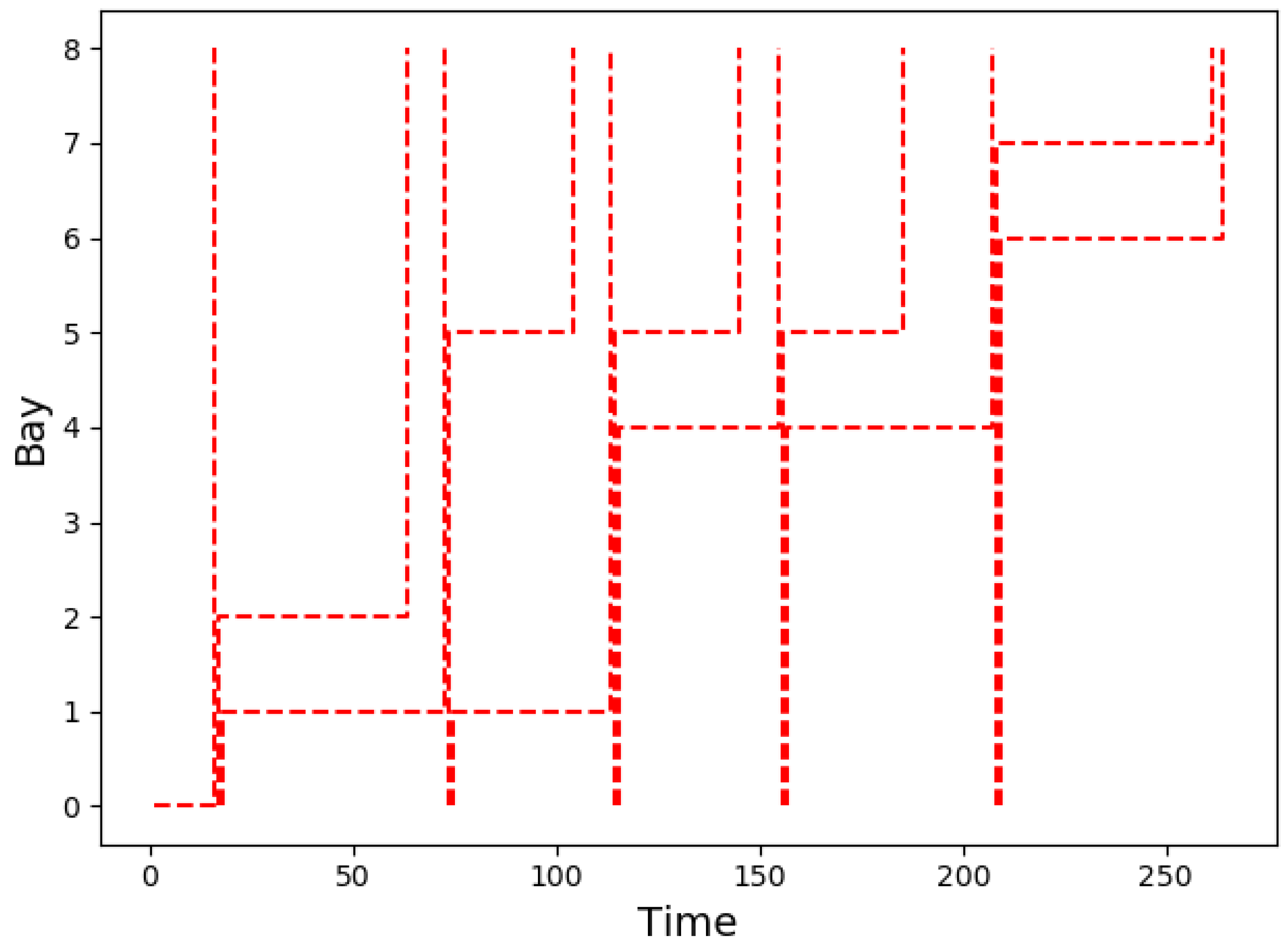
5.2. Numerical Example

This study is the first to discuss the hybrid scheduling of three types of equipment: AGV, YC and ET at the U-shape trafficked automated terminal. A feasible solution should not only satisfy the path constraint of AGV and ET, but also applies to the coupling relationship among AGV, ET and YC.

Table 6. Solving speed.

n	Size	Completion Time (Seconds)	CPU Time (Seconds)
	NC × NAGV
1	20 × 4	390	0.00
2	100 × 8	1948	0.00
3	200 × 8	3529	0.25
4	500 × 16	9344	0.26
5	1000 × 16	18,108	0.27
6	2000 × 32	36,624	0.40
7	10,000 × 48	185,879	0.55

shows the solving speed of feasible solutions under different number of containers and AGVs, where N_C denotes the number of containers, N_AGV denotes AGV quantity, “Completion Time” denotes the completion time of the transportation and “CPU Time” denotes the calculation time required for the solution, and the result is rounded to two decimal places. It can be seen that the actual calculation time for solving the model in this paper is still controlled within 1 s after the container reaches 10,000. Due to the fast solving speed of feasible solutions in this paper, the following mainly verifies the superiority of CCPSO by comparing the optimal solutions obtained by different algorithms in different container numbers, different AGV numbers and different iterations.

The feasibility of the model and algorithm were verified in this paper. Appendix

Table A1. Numerical example: general tasks information.

NC	Type	Block	Bay	Row	Fall
1	4	1	4	2	5
2	1	0	3	1	5
3	4	1	1	2	5
4	1	1	4	2	2
5	2	0	7	2	3
6	1	0	6	2	1
7	3	1	6	2	5
8	4	1	1	2	2
9	1	0	1	2	1
10	2	0	1	3	1
11	3	1	4	4	5
12	3	1	2	1	2
13	2	0	2	2	5
14	1	1	5	2	3
15	3	1	5	2	1
16	2	1	2	2	4
17	3	1	5	2	4
18	3	1	5	3	3
19	3	1	0	4	3
20	3	1	7	2	5

contains the task information that YC, AGV and ET need to perform in a small-scale calculation example containing 20 containers, where the number denotes the container number; the type denotes the task type of the current container; the block denotes the yard block number where the container is located; and the Bay, Row and Fall respectively denote the specific three-dimensional coordinate position of the container in the yard. The direction of Bay is parallel to YC carts. Appendix Table A1 shows the optimal scheduling arrangements of YC, AGV and ET after the solution is solved within 50 iterations. From the left-most column to the right-most column, the scheduling arrangement is two YCs at the No. 0 yard block, two YCs at No. 1 yard block, 4 AGVs and the queuing sequence of ET transporting corresponding containers at the entrance. Each column of Appendix

Table A2. Numerical experiment: allocation result of each equipment.

YC0	YC1	YC2	YC3	AGV0	AGV1	AGV2	AGV3	$\mathrm{ET}$
5	2	16	19	4	14	5	9	11
6	9	12	8	10	13	16	6	19
13	10	3	15	2				20
		17	1					18
		18	4					7
		14	11					12
		20	7					3
								8
								1
								15
								17

respectively indicates the order in which YC and AGV transport containers. The ET column indicates the order in which ET transporting the corresponding container enters the yard block, and the scheduling sequence is from top to bottom.

AppendixFigure A1, Figure A2, Figure A3 and Figure A4 show the positions and time relationships of AGV, ET, and YC at various times. The horizontal axis denotes time, and the vertical axis uses bay bits to denote the current position of each equipment along the track of YC cart. The layout of the yard is shown in Figure 3. The lanes of No. 1 block and No. 2 block are 0–7 and 8–14, respectively. In Appendix Figure A1, lines with four colors represent four different AGVs, respectively. Since ET does not belong to port internal equipment, the lines representing ET are all red in Appendix Figure A2. If the line crossing occurs at the same bay at the same time in Appendix Figure A1 and Figure A2, it means that there is a transport vehicle interference here. The entrance is assumed to be located at the 0-th bay. Due to the situation where the AGVs queue at the yard entrance, parallel lines appear at the 0 bay position in Appendix Figure A1, which means that the AGV of the corresponding color is waiting in the queue. There is no line crossing in Appendix Figure A1 and Figure A2, so it can be verified that the constraint model meets the requirements. Appendix Figure A4 shows the convergence of the optimal value of the algorithm in iterations. It can be seen that the optimal solution initially obtained is above 320 and then approaches to 285 after update iterations. In fact, the final solution result tends to be better as iteration increases, because CCPSO has the characteristic of not falling into local optimum. This characteristic will be further verified in subsequent experiments.

5.3. Simulation Comparison

To further verify the performance of CCPSO, different algorithms are calculated for comparison under different number of containers and AGVs. They include the traditional particle swarm optimization algorithm (PSO), the adaptive particle swarm optimization algorithm (APSO) developed by Cong et al. [22] and the random point particle swarm optimization algorithm (RPPSO) developed by Dawei et al. [28]. The particle processing method and fitness value solution models are based on the model in this study. All algorithms are calculated in the same iteration. Since the calculation time required in a single iteration of each algorithm is different, for each algorithm, we take the result at the same time point before the end of the calculation, rather than at the end of the iteration.

The velocity and position iteration method of PSO is based on (40) and (41). The percentage difference between PSO and CCPSO is represented by $GA{P}_{PSO-CCPSO}$ in (46). A positive result indicates that CCPSO is better, and a negative result indicates that PSO is better.

$$GA{P}_{PSO-CCPSO}=\frac{T_{PSO}-T_{CCPSO}}{T_{CCPSO}}\times 100(\%)$$

(46)

where $T_{PSO}$is the completion time of PSO, and $T_{CCPSO}$ is the completion time of CCPSO.

Similar to (46), the calculation formula for percentage deference between APSO, RPPSO and CCPSO is as follows:

$$GA{P}_{APSO-CCPSO}=\frac{T_{APSO}-T_{CCPSO}}{T_{CCPSO}}\times 100(\%)$$

(47)

$$GA{P}_{RPPSO-CCPSO}=\frac{T_{RPPSO}-T_{CCPSO}}{T_{CCPSO}}\times 100(\%)$$

(48)

where $T_{APSO}$ is the completion time of APSO, and $T_{RPPSO}$ is the completion time of RPPSO.

Appendix

Table A3. Comparison experiment of PSO, APSO, RPPSO and CCPSO.

n	Size	Completion Time (Unit Time)				GAP (%)
	${\mathit{N}}_{\mathit{c}}$$\times {\mathit{N}}_{\mathit{A}\mathit{G}\mathit{V}}$$\times {\mathit{N}}_{\mathit{I}}$	PSO	APSO	RPPSO	CCPSO	PSO	APSO	RPPSO
1	50 × 2 × 50	-	805	-	802	-	0.374	-
2	50 × 2 × 100	-	801	-	786	-	1.908	-
3	50 × 2 × 150	-	801	-	786	-	1.908	-
4	50 × 2 × 200	-	800	-	784	-	2.041	-
5	50 × 4 × 50	805	809	-	770	-	5.065	-
6	50 × 4 × 100	803	797	-	763	-	4.456	-
7	50 × 4 × 150	793	784	-	763	-	2.752	-
8	50 × 4 × 200	773	784	-	763	-	2.752	-
9	100 × 8 × 50	-	1808	1846	1795	-	0.724	2.841
10	100 × 8 × 100	-	1792	1826	1776	-	0.901	2.815
11	100 × 8 × 150	-	1781	1825	1773	-	0.451	2.933
12	100 × 8 × 200	-	1781	1825	1763	-	1.021	3.517
13	100 × 16 × 100	1795	1829	1831	1793	0.112	2.008	2.119
14	100 × 16 × 150	1805	1814	1812	1764	2.324	2.834	2.721
15	100 × 16 × 200	1773	1779	1811	1761	0.681	1.022	2.839
16	100 × 16 × 250	1763	1779	1800	1760	0.170	1.080	2.273
17	100 × 16 × 300	1763	1779	1800	1766	−0.170	0.736	1.925
18	100 × 16 × 350	1763	1779	1800	1755	0.456	1.368	2.564
19	200 × 8 × 50	3683	3680	3662	3658	0.683	0.601	0.109
20	200 × 8 × 150	3669	3626	3646	3581	2.457	1.257	1.815
21	200 × 8 × 250	3644	3578	3638	3560	2.360	0.506	2.191
22	200 × 8 × 550	3631	3574	3636	3555	2.138	0.534	2.278
23	200 × 8 × 650	3629	3574	3636	3555	2.082	0.534	2.278
24	200 × 8 × 750	3629	3574	3624	3578	1.425	−0.112	1.286
25	200 × 16 × 50	-	3652	3644	3585	-	1.869	1.646
26	200 × 16 × 150	-	3622	3637	3603	-	0.527	0.944
27	200 × 16 × 250	-	3585	3612	3563	-	0.617	1.375
28	200 × 16 × 550	-	3569	3607	3536	-	0.933	2.008
29	200 × 16 × 650	-	3569	3607	3536	-	0.933	2.008
30	200 × 16 × 750	-	3569	3607	3536	-	0.933	2.008
31	300 × 4 × 50	5746	-	5757	5709	0.648	-	0.841
32	300 × 4 × 150	5735	-	5736	5695	0.702	-	0.720
33	300 × 4 × 250	5732	-	5735	5662	1.236	-	1.289
34	300 × 4 × 550	5722	-	5713	5639	1.472	-	1.312
35	300 × 4 × 650	5689	-	5713	5627	1.102	-	1.528
36	300 × 4 × 750	5685	-	5713	5627	1.031	-	1.528
37	300 × 8 × 50	-	-	5727	5663	-	-	1.130
38	300 × 8 × 150	-	-	5679	5656	-	-	0.407
39	300 × 8 × 250	-	-	5679	5642	-	-	0.656
40	300 × 8 × 550	-	-	5679	5633	-	-	0.817
41	300 × 8 × 650	-	-	5651	5633	-	-	0.320
42	300 × 8 × 750	-	-	5651	5618	-	-	0.587
Average						1.162	1.418	1.695

gives the final task completion time of PSO, APSO, RPPSO and CCPSO under different container quantity, AGV numbers and iteration. In Appendix Table A3, each size ($N_c$×$N_{AGV}$×$N_I$) represents a group of experiments, and each group of experimental data is the average result of three independent experiments. In size ($N_c$×$N_{AGV}$×$N_I$), $N_I$ represents the maximum number of iterations. From Appendix Table A3, in the comparison simulation, the average gap of completion time can show the ability between CCPSO, PSO, APSO and RPPSO. It can find that CCSPO can save yard operation time about 1.162%, 1.418% and 1.695% more than others. Therefore, the searching ability of CCPSO is indeed better than other algorithms.

Figure 11 shows the comparison of the solution obtained by four algorithms under the same number of containers (N), different AGV number and maximum number of iteration. In each subgraph, the solid and dashed lines correspond to different AGV quantity, respectively. Different colors are used to indicate different algorithms respectively, and the corresponding relationship is as marked. Gray, orange, green and blue indicate PSO, APSO, RPPSO and CCPSO, respectively. It can be seen that the completion times obtained by CCPSO are basically below other lines in each subgraph, thus indicating that CCPSO’s solution results are better in most cases. When the number of containers increases, the solution of other algorithms gradually becomes flat, while the solution of CCPSO still maintains a downward trend, which means that CCPSO is more adaptable in complex situations and different allowed solution times. The experimental results show that CCPSO does not only find a near optimal solution in a short time, but also has a better ability to perform a global search.

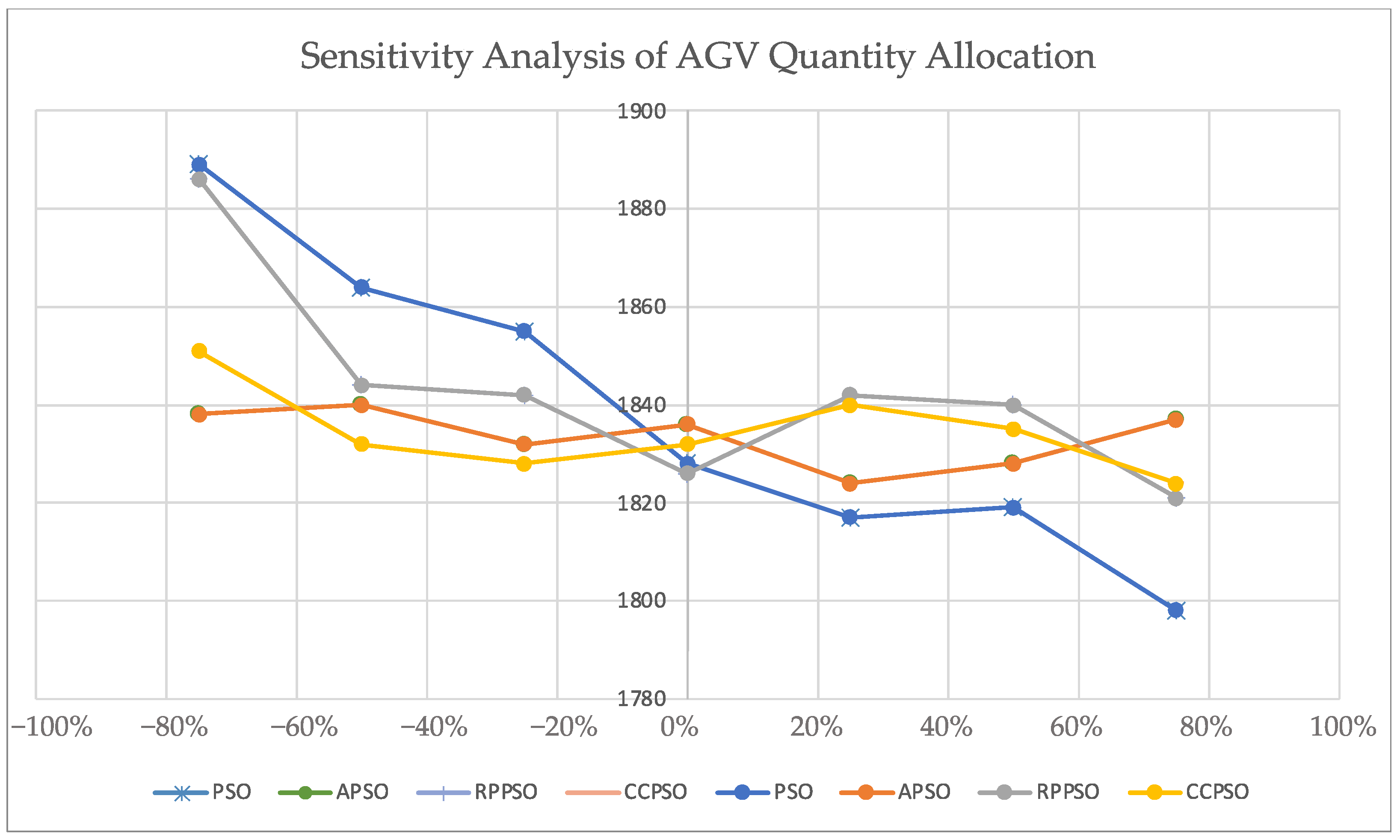
5.4. Sensitivity Analysis

The AGV quantity ($N_{AGV}$) and the iteration number ($N_I$) are considered separately as the sensitive sources, and the fitness values (completion times) of comparison algorithms are output.

In the sensitivity test of AGV quantity allocation, the total number of tasks is set to 100, the iteration number is set to 50 and the AGV allocation quantity 8′s change rate is set to 0%. The AGV detection rate (AGV quantity’s change rate) is −75%, −50%, −25%, 0%, 25%, 50% and 75%. The data obtained are shown in

Table 7. Sensitivity test data of AGV quantity allocation.

Size	$\mathbf{Detection}\mathbf{Rate}\left({\mathit{N}}_{\mathit{A}\mathit{G}\mathit{V}}\right)$	Completion Time (Unit Time)
${\mathit{N}}_{\mathit{c}}$$\times {\mathit{N}}_{\mathit{A}\mathit{G}\mathit{V}}$$\times {\mathit{N}}_{\mathit{I}}$		PSO	APSO	RPPSO	CCPSO
100 × 2 × 50	−75%	1889	1838	1886	1851
100 × 4 × 50	−50%	1864	1840	1844	1832
100 × 6 × 50	−25%	1855	1832	1842	1828
100 × 8 × 50	0%	1828	1836	1826	1832
100 × 10 × 50	25%	1817	1824	1842	1840
100 × 12 × 50	50%	1819	1828	1840	1835
100 × 16 × 50	75%	1798	1837	1821	1824

. Figure 12 shows the sensitivity of each algorithm when detecting results in different configurations of AGVs. It can be seen from Figure 12 that PSO’s results are sensitive to changes in the number of AGV. When the number of AGV quantity is small, the PSO’s results obtained are poor. When the AGV number increases, the PSO’s solution results are better than those of other algorithms. On the whole, the solution results of CCPSO are relatively stable, and at the same time, they are relatively close to the optimal results in the control group.

In the sensitivity test of the iteration number, the total number of tasks is set to 100, the AGV allocation quantity is set to 16 and the iteration number 200′s change rate is set to 0%. The iteration number’s detection rate (iteration number’s change rate) is −75%, −50%, −25%, 0%, 25%, 50% and 75%. The results obtained are shown in

Table 8. Sensitivity test data of iteration number.

Size	$\mathbf{Detection}\mathbf{Rate}\left({\mathit{N}}_{\mathit{A}\mathit{G}\mathit{V}}\right)$	Completion Time (Unit Time)
${\mathit{N}}_{\mathit{c}}$$\times {\mathit{N}}_{\mathit{A}\mathit{G}\mathit{V}}$$\times {\mathit{N}}_{\mathit{I}}$		PSO	APSO	RPPSO	CCPSO
100 × 16 × 50	−75%	1798	1837	1821	1824
100 × 16 × 100	−50%	1798	1812	1821	1824
100 × 16 × 150	−25%	1798	1807	1821	1822
100 × 16 × 200	0	1798	1801	1821	1787
100 × 16 × 250	25%	1798	1801	1821	1782
100 × 16 × 300	50%	1798	1801	1821	1779
100 × 16 × 350	75%	1798	1801	1821	1779

. As shown in Figure 13, CCPSO is most sensitive to the iteration number. When the iteration number increases, the result of CCPSO is better, while other algorithms do not appear to be insensitive. When the number of iterations increases, there are no further optimizations of these algorithms.

In summary, CCPSO has better adaptability in practical applications: when the allocation quantity of AGV is small, it can obtain a near-optimal solution in a shorter time; at the same time, CCPSO is sensitive to the iteration number. It can be seen that CCPSO has a better ability to search solutions and can adapt to different resource allocation and production requirements (it takes a shorter time to solve the near-optimal solution, or finds a better solution when the solution time is sufficient).

6. Conclusions

ZPMC proposed the U-shape trafficked terminal to improve the terminal efficiency. Meanwhile, it brought a new problem: mixed constraints between YC, AGV and ET in yard scheduling. A hybrid scheduling problem of YC AGV and ET at the U-shape trafficked terminal was studied. First, the scheduling objects involved in multi-equipment scheduling, such as YC, AGV and ET, were abstracted and formed into modules. Then each module was divided into four levels, according to its internal logical relationship: initialization layer, loop layer, particle module layer and scheduling module layers. Finally, a multi-equipment scheduling layered model architecture was established. The architecture, which has good scalability, is suitable for various multi-equipment hybrid scheduling problems. It can effectively avoid the duplication of work and improve research efficiency. A static and dynamic mixed scheduling method was put forward to solve the fitness value, which is suitable for the multi-equipment mixed constraint problem. The mapping space of decision variables to particles was optimized, and the CCPSO algorithm with particle chaos strategy and particle iterative speed control strategy was presented for the hybrid scheduling problem. The simulation experiment verifies the speed and effectiveness of the algorithm by using PSO, APSO, RPPSO and CCPSO for comparison. The comparative simulations are carried out under a different number of containers, different number of AGV and different maximum number of iterations. As the simulation showed, the CCSPO saves yard operation time about 1.162%, 1.418% and 1.695% better than PSO, APSO and RPPSO respectively, on average. The sensitivity test of AGV quantity and iteration number further shared the performance of CCPSO. The results show that, when the number of the container and AGV increases, the advantages of CCPSO are more obvious.

In the current work, we only considered the scheduling of one type of yard lane layout. In the future, the layout of multiple yard lanes will be considered. The scheduling of QCs will be considered, together with those of YCs, AGVs and ETs. This will involve more mixed constraints, such as AGV constraints from QCs to yards, YC non-crossing constraints, ET delays, etc. In addition, considering the inevitable uncertainty in terminal operations, the robust optimization [19] will also be considered.

References

1. Sun, Z.W. The world’s First! Zhenhua Heavy Industry Releases New Technology for Container Terminal Loading and Unloading, China Water Transport Network 2019. Available online: http://app.zgsyb.com/news.html?aid=530549 (accessed on 1 October 2021).
2. Beibu Gulf Port. Qinzhou Port Automated Container Terminal Completed Renovation. 2021. Available online: https://www.bbwport.cn/a/xinwenzixun/gongsixinwen/938.html (accessed on 1 October 2021).
3. Bowei, X.; Depei, J.; Junjun, L.; Yongsheng, Y.; Furong, W.; Haitao, S. A hybrid dynamic method for conflict-free integrated scheduling optimization in U-shaped automated container terminals. Comput. Ind. Eng. 2021, 162, 107695. [Google Scholar] [CrossRef]
4. Iris, C.; Lam, J.S.L. A review of energy efficiency in ports: Operational strategies, technologies and energy management systems. Renew. Sustain. Energy Rev. 2019, 112, 170–182. [Google Scholar] [CrossRef]
5. Bish, E.K.; Leong, T.Y.; Li, C.L.; Ng, J.W.C.; Simchi-Levi, D. Analysis of a new vehicle scheduling and location problem. John Wiley Sons Ltd. 2001, 48, 363–385. [Google Scholar] [CrossRef]
6. Bish, E.K. A multiple-crane-constrained scheduling problem in a container terminal. Eur. J. Oper. Res. 2003, 144, 83–107. [Google Scholar] [CrossRef]
7. Heuermann, A.; Duin, H.; Gorldt, C.; Thoben, K.-D. A Concept for Predictability and Adaptability in Maritime Container Supply Chains. In Dynamics in Logistics, LDIC 2018; Freitag, M., Kotzab, H., Pannek, J., Eds.; Springer: Cham, Switzerland, 2018. [Google Scholar] [CrossRef]
8. Boysen, N.; Briskorn, D.; Meisel, F. A generalized classification scheme for crane scheduling with interference. Eur. J. Oper. Res. 2017, 258, 343–357. [Google Scholar] [CrossRef]
9. Ehleiter, A.; Jaehn, F. Scheduling crossover cranes at container terminals during seaside peak times. J. Heuristics 2018, 24, 899–932. [Google Scholar] [CrossRef]
10. Eilken, A. A decomposition-based approach to the scheduling of identical automated yard cranes at container terminals. J. Sched. 2019, 22, 517–541. [Google Scholar] [CrossRef]
11. Briskorn, D.; Zey, L. Interference aware scheduling of triple-crossover-cranes. J. Sched. 2020, 23, 465–485. [Google Scholar] [CrossRef]
12. Zheng, F.; Man, X.; Chu, F.; Liu, M.; Chu, C. Two Yard Crane Scheduling With Dynamic Processing Time and Interference. IEEE Trans. Intell. Transp. Syst. 2018, 19, 3775–3784. [Google Scholar] [CrossRef]
13. Dik, G.; Kozan, E. A flexible crane scheduling methodology for container terminals. Flex. Serv. Manuf. J. 2017, 29, 64–96. [Google Scholar] [CrossRef]
14. Zhong, M.; Yang, Y.; Dessouky, Y.; Postolache, O. Multi-AGV scheduling for conflict-free path planning in automated container terminals. Comput. Ind. Eng. 2020, 142, 106371. [Google Scholar] [CrossRef]
15. Hu, H.; Jia, X.; He, Q.; Fu, S.; Liu, K. Deep reinforcement learning based AGVs real-time scheduling with mixed rule for flexible shop floor in industry 4.0. Comput. Ind. Eng. 2020, 149, 106749. [Google Scholar] [CrossRef]
16. Iris, C.; Christensen, J.; Pacino, D.; Ropke, S. Flexible ship loading problem with transfer vehicle assignment and scheduling. Transp. Res. Part B-Methodol. 2018, 111, 113–134. [Google Scholar] [CrossRef] [Green Version]
17. Chen, X.; He, S.; Zhang, Y.; Tong, L.; Shang, P.; Zhou, X. Yard crane and AGV scheduling in automated container terminal: A multi-robot task allocation framework. Transp. Res. Part C 2020, 114, 241–271. [Google Scholar] [CrossRef]
18. Houming, F.; Zhenfeng, G.; Lijun, Y.; Mengzhi, M. Combined configuration and scheduling optimization of dual trolley quayside crane and AGV in container terminal considering energy saving. Acta Autom. Sin. 2021, 45, 1–16. [Google Scholar]
19. Iris, C.; Lam, J.S.L. Recoverable robustness in weekly berth and quay crane planning. Transp. Res. Part B-Methodol. 2019, 122, 365–389. [Google Scholar] [CrossRef]
20. He, J.; Huang, Y.; Yan, W.; Wang, S. Integrated internal truck, yard crane and quay crane scheduling in a container terminal considering energy consumption. Expert Syst. Appl. 2015, 42, 2464–2487. [Google Scholar] [CrossRef]
21. Shyalika, C.; Silva, T.; Karunananda, A. Reinforcement Learning in Dynamic Task Scheduling: A Review. SN Comput. Sci. 2020, 1, 306. [Google Scholar] [CrossRef]
22. Cong, H.D.; Hop, V.N.; Anh, T.T.M. Adaptive particle swarm optimization for integrated quay crane and yard truck scheduling problem. Comput. Ind. Eng. 2020, 153, 107075. [Google Scholar]
23. Tang, L.X.; Zhao, J.; Liu, J.Y. Modeling and solution of the joint quay crane and truck scheduling problem. Eur. J. Oper. Res. 2014, 236, 978–990. [Google Scholar] [CrossRef]
24. Wei, J.; Li, Z.; You, L.; Guo, Y.; Tang, Z.; Hu, Z. Consider elite chaotic search strategy of indoor pedestrian evacuation model. J. Syst. Simul. 2021, 33, 1609–1616. [Google Scholar]
25. Yang, K.; Nomura, H. Quantum-Behaved Particle Swarm Optimization with Chaotic Search. IEICE Trans. Inf. Syst. 2008, E91-D, 1963–1970. [Google Scholar]
26. Chai, Z.J.; Ouyang, Z.H.; Li, Z. Improved analysis of multi-objective particle swarm optimization based on Henon chaotic mapping. Ordnance Ind. Autom. 2020, 39, 48–52. [Google Scholar]
27. Feng, J.; Zhang, J.; Zhu, X.; Lian, W. A novel chaos optimization algorithm. Multimed. Tools Appl. 2017, 76, 17405–17436. [Google Scholar] [CrossRef]
28. Zhou, D.; Gao, X.; Liu, G.; Liu, Y. Randomization in particle swarm optimization for global search ability. Expert Syst. Appl. 2011, 38, 15356–15364. [Google Scholar] [CrossRef]
Figure 1. Traditional automated terminal.
Jmse 09 01080 g001
Figure 2. U-shape trafficked automated terminal.
Jmse 09 01080 g002
Figure 3. U-shape trafficked container yard layout.
Jmse 09 01080 g003
Figure 4. Layered architecture.
Jmse 09 01080 g004
Figure 5. Constraint relationship of YC, AGV and ET.
Jmse 09 01080 g005
Figure 6. Dynamic process.
Jmse 09 01080 g006
Figure 7. A set of algorithm particles.
Jmse 09 01080 g007
Figure 8. CCPSO flowchart.
Jmse 09 01080 g008
Figure 9. Module layer process.
Jmse 09 01080 g009
Figure 10. Dynamic solving process.
Jmse 09 01080 g010
Figure 11. Comparison chart for PSO, APSO, RPPSO and CCPSO.
Jmse 09 01080 g011
Figure 12. Sensitivity analysis of AGV quantity allocation.
Jmse 09 01080 g012
Figure 13. Sensitivity analysis of iteration number.
Jmse 09 01080 g013