
Greenhouse Gas Emission Model for Tidal Flats in the Republic of Korea


1
Research Centre for Climate Change and Energy, Department of Environmental Sciences and Biotechnology, Hallym University, Chuncheon 24252, Korea
2
Research and Development Program Department, Korea Institute of Ocean Science and Technology, Busan 49111, Korea
3
Global Change Impact Studies Centre, Ministry of Climate Change, Government of Pakistan, Islamabad 44000, Pakistan
4
Center for Bio-Resource, Institute for Advanced Engineering, Yongin-si 17180, Korea
*
Author to whom correspondence should be addressed.
J. Mar. Sci. Eng. 2021, 9(11), 1181; https://0-doi-org.brum.beds.ac.uk/10.3390/jmse9111181
Submission received: 31 August 2021
/
Revised: 22 October 2021
/
Accepted: 23 October 2021
/
Published: 27 October 2021
(This article belongs to the Special Issue Coastal Wetlands)
Abstract
:Since coastal wetlands have been severely degraded and polluted by human activities, they have increasingly become a significant source of greenhouse gases (GHGs), so understanding the characteristics of their emissions is critical for devising future climate change mitigation strategies. This study modified a model based on carbon balance to forecast carbon stored and CO2, CH4 emissions in four types of typical tidal flats—Phragmites australis (PA), Spartina alterniflora (SA), Suaeda japonica (SJ), and Bare Tidal Flat (BTF) in Korea’s Ganghwa province from 2017 to 2047. The model was built using biomass data from salt plant species collected in different locations. The results indicate that the total annual simulated flow of CH4 increased over time in all four areas, most notably in SA, while CO2 remained relatively stable. The mean CO2 and CH4 fluxes in the four types of representative tidal flats were in the range of 0.03 to 19.1 mg m−2 d−1 and 0.007 to 5.23 mg m−2 d−1, respectively, across all seasons. Besides, the results indicate that the amount of carbon accumulated in the top soil increases linearly over time in nearly all areas studied, ranging from 0.01 to 0.13 (kgC m−2 yr−1). In general, the study provides a model for Korean tidal flats that incorporates carbon storage and GHG emissions in the intertidal zone in order to develop potential GHG reduction scenarios.
1. Introduction
A tidal flat acts both as a carbon sink, by storing carbon in sediment and vegetation, and as a carbon source, by releasing major greenhouse gases such as CO2 and CH4 into the atmosphere [1]. CO2 is fixed by plants and autotrophs through photosynthesis to form long-time storage organic compounds in plants and soil, a process known as carbon sequestration [2]. Recent studies have shown that the decomposition of soil organic matter is slow in the coastal wetland system because of anaerobic conditions in saturated sediments and salinity of the soil and water [3,4,5], however, decomposition still takes place through aerobic and anaerobic processes that produce CO2 and CH4 [6].
The median organic carbon stock sequestrated in the Korean tidal flats is 65.98 t C ha−1 in vegetated areas, and 53.91 t C ha−1 in barren areas [7], and the total amount of carbon stored in soil in the intertidal flats is approximately 6373.4 Gg [8]. Besides, statistics on GHG emissions from the tidal flats in Korea are also receiving great concern from researchers. According to a study carried out in 2016, the potential tidal flats emission corresponds to around 55.53 × 10⁶ t CO2e [6]. Chen et al. reported CO2 and CH4 emissions at tidal flat types of the Yellow River Delta wetlands with mean fluxes of −20.98 to 68.12 mg m−2 h−1 and −0.12 to 0.44 mg m−2 h−1 [9]. Thus, the investigation of carbon dynamics in the tidal flat area plays an important role in management, however, Korean tidal flats are a dynamic environment in which various processes such as tides, waves and precipitation interact to control the sedimentation in a complicated manner [10]. The large variation in space and time makes it difficult to determine the amount of carbon stored in the sediment and the emission quantities from the tidal flat. Direct measurement of CO2 and CH4 emissions using chamber or sediment sampling at defined areas provide essential information on a location basis over a period of time and defined space. However, due to the diversity of variables, such as soil, climate, and vegetation, it is difficult to generalize this information on a larger scale [11]. Therefore, the development of a model based on the interactive reactions of the biochemical processes in the carbon cycle is necessary to calculate the amount of CO2 and CH4 released from tidal flats.
Currently, soil carbon dynamics are simulated using a variety of models, including RothC, Century, and ICBM (Introductory Carbon Balance Model) [12,13,14]. In the majority of treatments, these models confidently predicted long-term trends. All of these models have been validated in a variety of climate zones around the world, and the results indicate that the more complex models employ between four (RothC) and six (Century) (more or less) dynamic soil carbon pools, and have sufficient complexity to at least attempt to model short-term dynamics (on the order of weeks and months). The simplest models (such as ICBM) that are capable of simulating long-term dynamics over several decades make use of a single dynamic pool [15]. Admittedly, models for predicting carbon dynamics in tidal flat areas are limited and are attracting considerable attention from scientists.
This study modified the ICBM (Introductory Carbon Balance Model) and applied it to provide simulation results of GHG emitted from Tidal Flat over the period of 2017 and 2047. Since ICBM has been regarded as one of the excellent models to simulate carbon dynamics in soil, it has been extensively applied to estimate the amount of carbon stored in agricultural soils over a long period to establish the efficient and effective soil management plans [16,17,18]. The main objectives of this study were to improve the ICBM, to optimize the model parameters in accordance with a tidal flat area, and to evaluate the applicability of the model to predict the amount of carbon stored in the sediment and GHG emissions (CO2 and CH4) over 30 years from 2017 to 2047, using data from the vegetated tidal flat and BTF areas in Ganghwa, Korea. The main advantage of developing such a process-based model is to forecast GHG emissions quantitatively, offering suitable management practices.
2. Materials and Methods
2.1. Model Description
This model named as Greenhouse Emission Model for Blue Carbon (GEM_BC) is based on the carbon mass balance to simulate the carbon dynamics in tidal flat layers. The model assumes that the tidal flat layer is composed of two layers: young layer (YL), defined as the layer where organic carbons are decomposed biologically to generate CO2 only under aerobic conditions, and old layer (OL), defined as the layer where those emit CO2 and CH4 under anaerobic conditions.
To develop this model, it is essential to understand the variation of layer environment with time as well as organic carbon flows through the layers. Organic carbons originating from organic debris in the water layer would continuously be deposited on the YL. As already mentioned, CO2, one of the major GHG, is likely to be produced from the YL. Some organic carbons in the YL are resistant to biological decompositions that they may undergo humification process to accumulate carbon, leading to a gradual growth of the YL and eventually shifting to the OL. As the thickness of the YL increases, the air penetration would be limited below a certain depth, forming anaerobic conditions and thus turning the lowest part of the YL to the OL where anaerobic biological decomposition would be initiated to release CO2 and CH4 (Figure 1).
The conceptual model is expressed mathematically based on the following assumptions:
- ▪
- ▪
- External influence coefficient is relatively constant with time, assuming a steady external input [21].
- ▪
- Annual amount of carbon sequestration is accounted for by that in the total biomass of the one-year plants.
- ▪
- Lateral C flux: Currently, there are no specific research results on the lateral C flux in the tidal flat areas of Korea. Besides, the west coast of South Korea receives large amounts of sediment from rivers, it is considered a carbon sink [1]. This amount of carbon is mainly deposited in the tidal flat areas [8]. Therefore, the model assumed that the amount of carbon transported by the lateral C flux in the study areas is negligible.
2.1.1. Kinetic Equations
Kinetic equations are denoted for organic carbon dynamics in YL and OL as follows:
where C represents the areal amount of organic carbon (kgC m−2), i denotes the input rate of organic carbon to the YL (kgC m−2 yr−1), k21 denotes the decomposition rate constant in YL (yr−1), is the external influence coefficient, h is humification coefficient, k22 is decomposition rate constant in OL (yr−1). Subscripts 1 and 2 represent YL and OL, respectively.
Integration of Equations (1) and (2) allow the following expression for organic carbon content with time in YL and OL:
where C10 and C20 are initial values for C1 and C2, respectively.
In YL, soil carbon decomposes aerobically through microbial respiration, releasing CO2 into the atmosphere. The humification coefficient (h) controls the fraction of YL that enters OL and (1−h) then represents the fraction of the outflow from YL that directly becomes CO2-C (Figure 1). The CO2 emissions from YL is calculated using Equation (5):
where is CO2 emission from YL.
In OL, organic carbons are anaerobically decomposed to release CO2 and CH4. The study assumed a ratio of carbon sequestration (Cs) to carbon in CH4 (CH4_C) for PA, SA, SJ, and BTF areas in OL (see Table 1), based on the correlation between annual Cs and CH4 emissions investigated in tidal flat areas [7,22,23,24]. The CO2 and CH4 emissions from OL are calculated using Equations (6) and (7):
where is CO2 emission from OL. is CH4 emission from OL. 1/a is the ratio of CH4_C: Cs from OL.
2.1.2. Determination of Model Parameters
Five parameters (, k21, k22, i, and h) are needed to calculate the kinetic equation described in Section 2.1.1.
, denoting the eternal influences on soil organic matter decompositions rates of the tidal flat, depends on three main factors: (i) soil temperature factor (t), (ii) soil moisture factor (m), and (iii) soil salinity factor (s) of the tidal flat. The daily values for were calculated using the following equation: = t · m · s. In this equation, t and m were calculated from daily meteorological data and soil data following the approach in Andrén et al. [21] and Fortin et al. [25]. The s factor depends on the osmotic potential at the actual soil water content and electrical conductivity. The exponential relationship between microbial activity and salinity is determined by the formula given in Yuan et al. [26].
where (osmotic potential) was calculated by using: Os = -(EC1:5 × bulk density × 54)/soil water content.
Where EC1:5 is the electrical conductivity (dS.m−1) of 1:5 soil/water extract. The EC1:5 was converted from ECe using the equation proposed by Shaw et al. [27].
This study assumed the value of k21 and k22 as 0.8 yr−1 and 0.006 yr−1 following Andrén et al. [16].
The fourth parameter i in vegetated area is calculated following the formula provided in Howard et al. [1], where, Mi is the biomass of vegetation (kg m−2), CFi is carbon conversion factor for grasses, and At is the area occupied by vegetation community (m−2). In BTF area, the carbon source is mainly provided from the deposition of terrestrial sediments and suspended particles from seawater [8]. Thus, the annual carbon input was determined based on the mean C sequestration rate per year (kgC m−2 yr−1).
Lastly, h, denoting the proportion of young soil carbon that becomes sediment carbon (humus), is estimated following the formula: h = (hs · is + hr · ir)/i [16]. Where hs and hr are humification coefficient of stem and roots, while is and ir are carbon amount of stem and roots, respectively. In BTF area, the carbon can be considered as sewage sludge, so humification coefficient was set 0.41 [28].
2.2. Model Validation
The model’s simulation of topsoil carbon mass, CO2 and CH4 emissions were validated against observed data available from a study conducted by the Korea Marine Environment Management Corporation as part of the “Development of Blue Carbon Information System and its Assessment for management” project from Ganghwa-do (37.7° N, 126.5° E) [29], which encompasses the southern portion of the tidal flat. The study area is sandwiched between the Sukmo and Yeomha channels to the west and east, respectively, and thus receives a significant amount of carbon sediment annually. A layer of mud and salt plants covers most of its surface area. Numerous salt plants are found in the area, with three dominant species: Phragmites australis (PA), Spartina alterniflora (SA), and Suaeda japonica (SJ). The sampling areas, Yeochari, Dongmakri, and Donggeomdo which are homes to PA, SA, and SJ species, respectively, are located south of Ganghwado along the coastline. At Dongmakri, bare tidal flat soil carbon data were also collected (Figure 2).
2.3. Experimental Data
During the growing season (May to November) from 2017 to 2019, this study collected PA, SA, and SJ biomass data. The above-ground biomass estimation method makes use of a quadrat to represent sampling areas within plots following Howard et al. [1]. In this experiment, quadrats measured 50 cm × 50 cm in size. Stems were collected in each quadrat to determine the wet and dry weights. In the laboratory, wet weight stem biomass was oven-dried for approximately 72 h at 60 degrees Celsius to obtain a constant dry weight stem biomass.
This study used direct sampling to determine the biomass of the roots (below-ground biomass) and the samples were taken by extracting a core as described in Howard et al. [1]. Further, following methodology in Saunders et al. (2006), 10 cm diameter cores for sampling 2.5 cm wide segments cut at various depths of 2.5, 5, 7.5, 12.5, 15, 22.5, and 25 cm, and another sampling 5 cm wide segments cut at depths of 35, 45, 55, and 65 cm were used [30]. The segments were then visually separated into root, rhizome, and dead litter components after washing them over a 1 mm screen. The living and dead things were distinguished based on color [30]. Following that, living root and rhizome materials were oven-dried to a constant dry weight at 60 degrees Celsius. The below-ground biomass was then determined in the manner described by Howard et al. [1].
3. Results and Discussion
3.1. Input Data and Parameter Values in Ganghwa-do, Korea
Table 1 shows the data input for the model. Total biomass was calculated in vegetated areas using stem, roots, and rhizodeposition (the amount of biomass allocated to the soil during the growing season as root change and exudates). This study used Pausch et al. estimate of 68.75% root turnover for rhizodeposition, which is calculated by multiplying the estimated root biomass C by 0.6875 and adding that as C input from root turnover [31]. The halophytes that inhabit in Ganghwa are highly dependent on the weather conditions during the winter months. Despite minor differences, most juveniles emerge in early spring and grow until autumn. In the winter, they turn brown and cease to grow. Therefore, this study assumed that the entire C amount in biomass would be converted into annual carbon input to soil. SJ and PA are two common native plants in the Ganghwa area. Meanwhile, SA was first discovered near Dongmak Beach in 2012 [32], however, it has expanded, and the density of individuals is high (334 no. stem/m2), so the amount of carbon stored in this plant is greater than that of the other two species—SJ and PA. Optimization of the parameter h was done in accordance with the relative contribution of root versus shoot material to the formation of soil organic matter. The relative contribution of root versus stem material to soil was estimated using Kätterer et al. results [28]. According to the findings of Kätterer et al., root-derived material humifies 2.3 times faster than above-ground plant material [29]. The estimation factors for hs and hr are 0.15 and 0.35, respectively.
Among the most important factors influencing decomposition rates in soil are soil temperature and water content. Also, various studies show that increased salinity slows microbial degradation [26,33,34]. After having gathered the raw input data (see Table 1), this study analyzed the raw data to obtain the external factors parameter ϵ. For example, to calculate the effect of ϵm, evaporation (ETo) was calculated using equation 6 of Allen et al. and has an annual mean value of 2380 (mm) [35]; Pedotransfer functions were used to estimate the soil’s field capacity and wilting point [36], which were determined as 35% and 22%, respectively. Furthermore, the ECe data was gathered from the literature to determine the impact of soil salinity on the rate of decomposition [37]. Due to the study areas proximity and similar climatic conditions, the difference in mean value of ϵ is very close, and almost equal. In general, the value of ϵ represents the peak during the summer months, which is attributable to soil temperature and soil water content, and is usually low during the cold and dry winter months (see Figure A1).
3.2. Simulation of Topsoil Carbon Mass
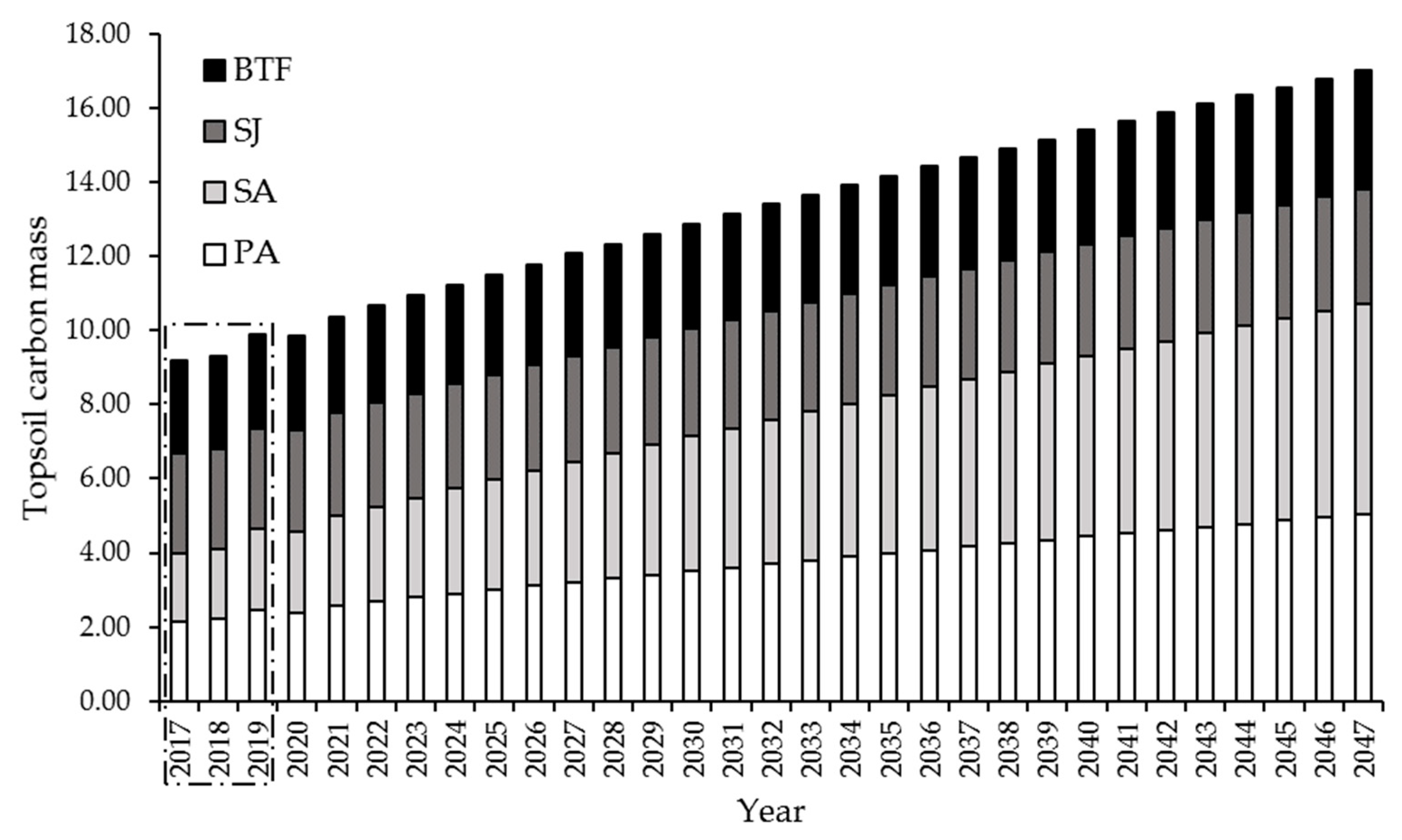
Figure 3 illustrates the model’s prediction results for the carbon content of the topsoil (0–25 cm depth) corresponding to halophyte types and BTF in the Ganghwa area from 2017 to 2047. As shown, the amount of carbon accumulated in the soil increases linearly over time in almost all of the areas studied. However, PA and SA predicted a significant increase in the amount of carbon accumulated in the soil. Specifically, the amount of carbon in the topsoil increased by an annual average of 0.1, 0.13, 0.01, and 0.02 (kgC m−2 yr−1), in the PA, SA, SJ, and BTF study areas, respectively. This depends largely on the amount of carbon that enters the ecosystem each year. According to the Blue Carbon Manual published by the IUCN (International Union for Conservation of Nature), the composition and density of vegetation in coastal wetlands have an impact on the total carbon stock [39]. Studies regarding the vegetated tidal flat area indicate that high sedimentary organic carbon content in salt marshes is primarily due to increased carbon input via plant litter and roots, as well as their location in saturated and, presumably, more anaerobic environments as opposed to other types of marshes [40]. For the BTF region, the increase in carbon in topsoil sediments was primarily due to organic carbon deposition from marine and terrestrial sources. The Ganghwa tidal flat, which is influenced by terrestrial inputs such as freshwater discharge, municipal sewage, and discharge, contributes to the burial of organic carbon in sediments [22]. All the relevant data related to Figure 3 is provided in Appendix A, Table A1.
For the purpose of validating the simulation results of the model, Figure 4 shows a comparison of the simulated and measured carbon stored in sediments at a depth of 25 cm in Ganghwa from 2017 to 2020, which was conducted at four different locations throughout the year. As illustrated in Figure 4, the annual carbon stored in the simulated sediment is generally consistent with the data collected from field sites at various points in time. Also, at some points the simulated magnitude is slightly different from the observed data, with observed carbon in sediments being higher or lower. This could be because tidal energy in a variety of topographical and morphological settings could be a critical factor in increasing not only the supply of waterborne sediment particles, but also organic carbon burial in intertidal sediments. Lee et al. demonstrated that the amount of sedimentary carbon varies over time and space due to a variety of factors such as wave, tidal, and erosion and coastal environments [22].
Thus, the unique parameter affecting the carbon mass in soil prediction results is i. Besides that, ϵ is a parameter that has a direct effect on the decomposition process. It is worth noting that this study did not account for carbon deposits from terrestrial inputs caused by riparian discharge into salt marshes, which could have a significant impact. Additionally, because of the scarcity of data, the model’s test results do not account for wave, tidal, or erosion effects, all of which contribute to annual carbon uncertainty.
3.3. Simulation of GHG Emissions
The simulation results for CO2 and CH4 emissions in all four test sites from 2017 to 2047 were as shown in Figure 5. Litter decomposition is the primary source of CO2, which is influenced by temperature and humidity. The results demonstrate that the annual carbon input and the external coefficient have a strong influence on the simulation results of CO2 emitted. The comparison of monthly simulated and observed soil CO2 emissions for the years 2019 at all four sites were as shown in Figure 6. Both prediction and measurement of CO2 emissions in the fields followed a similar pattern, with the highest levels of emissions being recorded during the May to August growing season. This could be because during the summer temperatures are high, resulting in increased respiration rates for roots and soil microorganisms. Although the data are only for seasonally specific months, the CO2 emissions predictions are comparable to the measured. However, the observed and simulated daily fluxes differ in terms of peak timing and magnitude. The model’s CO2 emission peak occurs in May for all regions as follows; 7.61 mg m−2 day−1 for PA, 7.92 mg m−2 day−1 for SA, 6.03 mg m−2 day−1 for SJ, and 0.83 mg m−2 day−1 for BTF. This is because the applicable sites are in close proximity to one another, implying that the natural conditions are similar. Meanwhile, the areas PA and BTF have emission peaks of 12 mgCO2-C m−2 day−1, and 11 mgCO2-C m−2 day−1 in August, while the SA and BTF areas have emission peaks of 11 mgCO2-C m−2 day−1 in May.
CH4 is produced during the degradation of organic matter in anaerobic (OL) conditions. The major factors affecting the amount of CH4 released are dissolved organic carbon (DOC) and soil moisture. Carbon input and methanogenic activity are correlated positively, i.e., increase in carbon input from biomass and exudates results to increase in methane production [41]. Thus, the more DOC sediment present, the more CH4 is released. According to Figure 5, the amount of CH4 released in the PA and SA areas increases over time, owing to the increase in carbon accumulated in the sediment. In comparison, CH4 emissions decreased in the BTF and SJ regions, owing to the region’s low annual carbon input, which is insufficient to compensate for the amount of sediment degraded by microbial decomposition activities. Figure 6 illustrates the comparison of simulated and observed values in various vegetative areas in 2019. Although the DOC has a significant positive correlation with CH4 emissions, Kim et al. assert that it has no direct effect on CH4 emissions [41]. The dependence on DOC and soil moisture results in a proportional increase in bacteria that reduce sulfate, thereby affecting CH4 emissions [41]. Sulfate-reducing bacteria competitively inhibits methanogenic activities which are the primary source of CH4 [42]. The composition and quality of carbon sources have a significant effect on the structure of the methanogen-generating community [43], and thus the amount of CH4 released varies based on salt plant regions. Recent studies report that the potential for methane production is greater in SA regions than in PA, SJ, and BTF regions, owing to the influence of microbiological content, water table, and depth [23,40,41]. In comparison to the observed values, the simulated CH4 concentration in winter months was highly consistent, whereas the simulated results for the growing season in the PA, SJ, and BTF areas were generally higher.
In general, the simulation results of the model show a significant increase in CH4 emissions in the future, while CO2 emissions will remain relatively stable. The main reason is due to increased sequestration of carbon in the sediments. The difference between simulation and observed results is due to cross factors that contribute to the uncertainty of the model such as tides, changes in salinity, content of microbial enzymes, etc. as well as factors affecting the change in carbon content in sediments.
4. Conclusions
This study developed the GHG Emissions Model for tidal flat areas to make estimates of CO2 and CH4 emissions based on the carbon balance of the carbon sink. The model of Tidal Flat GHG emissions has been verified using annual carbon accumulation in sediment from 2017 to 2020 and daily CO2 and CH4 emissions in 2019 from four different locations in Ganghwa, Korea. The results indicate that, in comparison to 2017, CH4 emissions in the PA and SA areas have increased over time due to increased carbon accumulation in the sediment. In comparison, the results of the simulations in the SJ and BTF regions remained relatively stable over time. CO2 emissions from sites also remained relatively stable over time. The study demonstrated that the model is capable of capturing significant trends in soil CO2 and CH4 emissions under natural conditions in Ganghwa, Korea. According to the results of the simulated and observed comparisons, CO2 and CH4 emissions occur primarily during the growing season, while are near zero in most areas during the winter. Following an examination of the relationship between carbon sequestration and GHG emissions, the tidal flat ecosystem is critical for carbon sequestration.
The simulation results were generally consistent with the corresponding experimental data under the model application conditions. However, when peak time and magnitude differences between observed and daily flux simulations were compared, the modeling simulation did not completely match the measured values. This is because the model’s experimental results did not account for the amount of carbon deposited by terrestrial currents that accumulate in salt marshes areas, the effects of tides, erosion on soil carbon content, and salinity variation (limitations of study). This causes uncertainty in the annual carbon input and also affect the model’s simulation results. Therefore, a detailed study of lateral C flow and carbon deposition in the experimental areas is required to determine the amount of carbon added or eroded in the topsoil layer, from which the model’s simulations can be run more precisely. To obtain more accurate predictions of CO2 and CH4 emissions, the model must be refined further by incorporating wave energy, water tide, and the correlation between gas volume emission and the enzyme content of the microorganisms involved. Also, salinity is a dynamic property of the soil that changes in response to environmental factors, however, this study assumed it as a constant. Due to the complexity of the processes involved in the development of salinity and the scarcity of data, it is impossible to calculate the uncertainty associated with electrical conductivity (EC) measurements.
In conclusion, the model forecasted carbon dynamics until 2047 for Korea’s tidal flats, including carbon storage and GHG emissions in the intertidal zone, for future management scenarios. Further research is recommended to consider additional methods (such as DMI, GLUE etc.) for reducing the model’s uncertainty, and it can also be extended by applying it to other areas of the Korean coastal ecosystem (salt marshes and BTF). To continue developing the model, it could be extended in the future to fully establish the processes involved in the carbon cycle in the blue carbon field.
Author Contributions
Conceptualization, N.Y.T.D. and S.K.; Methodology, N.Y.T.D. and H.-S.P.; Formal analysis, N.Y.T.D. and K.A.M.; Data Curation, H.-S.P. and C.-G.K.; Writing—Original Draft, N.Y.T.D.; Writing—Review and Editing, H.-S.P., K.A.M., C.-G.K. and S.K.; Visualization, N.Y.T.D. and K.A.M.; Supervision, S.K.; Project administration, S.K.; Funding acquisition, S.K. All authors have read and agreed to the published version of the manuscript.
Funding
This research was funded by the Korea Ministry of Oceans and Fisheries under the project Development of Blue Carbon Information System and its Assessment for Management (grant number 20170318) and the Korea Ministry of Environment as Waste to Energy-Recycling Human Resource Development Project (grant number YL-WE-21-001).
Institutional Review Board Statement
Not applicable.
Informed Consent Statement
Not applicable.
Data Availability Statement
All the raw data used in this study was obtained from Korea Marine Environment Management Corporation (https://www.koem.or.kr/site/eng/main.do, accessed on 6 Janurary 2021). All the remaining data is provided in the tables and figures of the main article and appendix. Further inquiries can be directed to the corresponding author.
Acknowledgments
We would like to express our gratitude to Korea Marine Environment Management Corporation for providing the data used to validate the model as part of the Development of Blue Carbon Information System and its Assessment for Management program. The authors would also like to thank the reviewers and the journal’s editor for their valuable comments, which have greatly improved the study.
Conflicts of Interest
The authors declare no conflict of interest. The funders had no role in the design of the study; in the collection, analyses, or interpretation of data; in the writing of the manuscript, or in the decision to publish the results.
Appendix A
Table A1. Model projections (2017–2047) of soil carbon mass (kgC m−2 yr−1) at 25 cm depth at the four experimental sites in Ganghwa province of Korea. Table A2. Simulation of CO2 emissions (kg ha−1 yr−1) over years at the four experimental sites in Ganghwa province of Korea. Table A3. Simulation of CH4 emissions (kg ha−1 yr−1) over years at the four experimental sites in Ganghwa province of Korea. Figure A1. Mean within 4 years (2017–2020) dynamics of ϵ in Ganghwa, Korea.

Table A1.
Model projections (2017–2047) of soil carbon mass (kgC m−2 yr−1) at 25 cm depth at the four experimental sites in Ganghwa province of Korea.
Table A1.
Model projections (2017–2047) of soil carbon mass (kgC m−2 yr−1) at 25 cm depth at the four experimental sites in Ganghwa province of Korea.
| Sites | 2017 | 2018 | 2019 | 2020 | 2021 | 2022 | 2023 | 2024 | 2025 | 2026 | 2027 |
| PA | 2.14 | 2.23 | 2.47 | 2.39 | 2.58 | 2.68 | 2.79 | 2.89 | 3.00 | 3.10 | 3.20 |
| SA | 1.84 | 1.88 | 2.16 | 2.19 | 2.42 | 2.56 | 2.70 | 2.84 | 2.97 | 3.11 | 3.25 |
| SJ | 2.73 | 2.69 | 2.71 | 2.73 | 2.78 | 2.80 | 2.81 | 2.83 | 2.84 | 2.85 | 2.87 |
| BTF | 2.49 | 2.52 | 2.56 | 2.56 | 2.60 | 2.63 | 2.65 | 2.68 | 2.71 | 2.73 | 2.76 |
| 2028 | 2029 | 2030 | 2031 | 2032 | 2033 | 2034 | 2035 | 2036 | 2037 | 2038 | |
| PA | 3.30 | 3.40 | 3.50 | 3.60 | 3.69 | 3.79 | 3.89 | 3.98 | 4.07 | 4.16 | 4.25 |
| SA | 3.38 | 3.51 | 3.64 | 3.77 | 3.90 | 4.02 | 4.15 | 4.27 | 4.40 | 4.52 | 4.64 |
| SJ | 2.88 | 2.89 | 2.91 | 2.92 | 2.93 | 2.94 | 2.96 | 2.97 | 2.98 | 2.99 | 3.00 |
| BTF | 2.78 | 2.81 | 2.83 | 2.85 | 2.88 | 2.90 | 2.93 | 2.95 | 2.97 | 2.99 | 3.02 |
| 2039 | 2040 | 2041 | 2042 | 2043 | 2044 | 2045 | 2046 | 2047 | |||
| PA | 4.34 | 4.43 | 4.52 | 4.61 | 4.70 | 4.78 | 4.87 | 4.95 | 5.03 | ||
| SA | 4.76 | 4.88 | 4.99 | 5.11 | 5.22 | 5.34 | 5.45 | 5.56 | 5.67 | ||
| SJ | 3.02 | 3.03 | 3.04 | 3.05 | 3.06 | 3.07 | 3.09 | 3.10 | 3.11 | ||
| BTF | 3.04 | 3.06 | 3.08 | 3.11 | 3.13 | 3.15 | 3.17 | 3.19 | 3.21 |
Table A2.
Simulation of CO2 emissions (kg ha−1 yr−1) over years at the four experimental sites in Ganghwa province of Korea.
Table A2.
Simulation of CO2 emissions (kg ha−1 yr−1) over years at the four experimental sites in Ganghwa province of Korea.
| Sites | 2017 | 2018 | 2019 | 2020 | 2021 | 2022 | 2023 | 2024 | 2025 | 2026 | 2027 |
| PA | 16.82 | 16.86 | 16.90 | 16.94 | 16.98 | 17.02 | 17.05 | 17.09 | 17.13 | 17.17 | 17.20 |
| SA | 19.84 | 19.90 | 19.95 | 20.00 | 20.05 | 20.10 | 20.15 | 20.20 | 20.25 | 20.30 | 20.35 |
| SJ | 6.14 | 6.15 | 6.16 | 6.16 | 6.17 | 6.17 | 6.18 | 6.18 | 6.19 | 6.19 | 6.20 |
| BTF | 0.90 | 0.91 | 0.92 | 0.93 | 0.94 | 0.94 | 0.95 | 0.96 | 0.97 | 0.98 | 0.99 |
| 2028 | 2029 | 2030 | 2031 | 2032 | 2033 | 2034 | 2035 | 2036 | 2037 | 2038 | |
| PA | 17.24 | 17.28 | 17.31 | 17.35 | 17.38 | 17.42 | 17.45 | 17.49 | 17.52 | 17.55 | 17.59 |
| SA | 20.40 | 20.45 | 20.49 | 20.54 | 20.58 | 20.63 | 20.68 | 20.72 | 20.76 | 20.81 | 20.85 |
| SJ | 6.20 | 6.21 | 6.21 | 6.21 | 6.22 | 6.22 | 6.23 | 6.23 | 6.24 | 6.24 | 6.25 |
| BTF | 0.99 | 1.00 | 1.01 | 1.02 | 1.02 | 1.03 | 1.04 | 1.05 | 1.05 | 1.06 | 1.07 |
| 2039 | 2040 | 2041 | 2042 | 2043 | 2044 | 2045 | 2046 | 2047 | |||
| PA | 17.62 | 17.65 | 17.69 | 17.72 | 17.75 | 17.78 | 17.81 | 17.84 | 17.87 | ||
| SA | 20.89 | 20.94 | 20.98 | 21.02 | 21.06 | 21.10 | 21.14 | 21.18 | 21.22 | ||
| SJ | 6.25 | 6.26 | 6.26 | 6.26 | 6.27 | 6.27 | 6.28 | 6.28 | 6.28 | ||
| BTF | 1.08 | 1.08 | 1.09 | 1.10 | 1.10 | 1.11 | 1.12 | 1.12 | 1.13 |
Table A3.
Simulation of CH4 emissions (kg ha−1 yr−1) over years at the four experimental sites in Ganghwa province of Korea.
Table A3.
Simulation of CH4 emissions (kg ha−1 yr−1) over years at the four experimental sites in Ganghwa province of Korea.
| Sites | 2017 | 2018 | 2019 | 2020 | 2021 | 2022 | 2023 | 2024 | 2025 | 2026 | 2027 |
| PA | 1.747 | 1.861 | 1.973 | 2.084 | 2.194 | 2.303 | 2.410 | 2.517 | 2.623 | 2.727 | 2.831 |
| SA | 4.012 | 4.459 | 4.902 | 5.340 | 5.774 | 6.203 | 6.628 | 7.050 | 7.466 | 7.879 | 8.288 |
| SJ | 2.190 | 2.202 | 2.214 | 2.226 | 2.238 | 2.250 | 2.262 | 2.274 | 2.285 | 2.297 | 2.308 |
| BTF | 1.176 | 1.188 | 1.199 | 1.211 | 1.222 | 1.233 | 1.244 | 1.255 | 1.266 | 1.277 | 1.287 |
| 2028 | 2029 | 2030 | 2031 | 2032 | 2033 | 2034 | 2035 | 2036 | 2037 | 2038 | |
| PA | 2.933 | 3.035 | 3.135 | 3.235 | 3.333 | 3.431 | 3.527 | 3.623 | 3.717 | 3.811 | 3.904 |
| SA | 8.692 | 9.092 | 9.489 | 9.881 | 10.27 | 10.65 | 11.04 | 11.41 | 11.79 | 12.16 | 12.52 |
| SJ | 2.319 | 2.330 | 2.341 | 2.352 | 2.363 | 2.373 | 2.384 | 2.394 | 2.405 | 2.415 | 2.425 |
| BTF | 1.298 | 1.308 | 1.319 | 1.329 | 1.339 | 1.349 | 1.359 | 1.369 | 1.378 | 1.388 | 1.397 |
| 2039 | 2040 | 2041 | 2042 | 2043 | 2044 | 2045 | 2046 | 2047 | |||
| PA | 3.996 | 4.086 | 4.176 | 4.266 | 4.354 | 4.441 | 4.527 | 4.613 | 4.698 | ||
| SA | 12.88 | 13.24 | 13.60 | 13.95 | 14.30 | 14.64 | 14.98 | 15.32 | 15.65 | ||
| SJ | 2.435 | 2.445 | 2.455 | 2.465 | 2.474 | 2.484 | 2.493 | 2.503 | 2.512 | ||
| BTF | 1.407 | 1.416 | 1.425 | 1.434 | 1.444 | 1.452 | 1.461 | 1.470 | 1.479 |
Figure A1.
Mean within 4 years (2017–2020) dynamics of ϵ in Ganghwa province, Korea.

References
- Howard, J.; Hoyt, S.; Isensee, K.; Telszewski, M.; Pidgeon, E. (Eds.) Coastal Blue Carbon: Methods For Assessing Carbon Stocks And Emissions Factors In Mangroves, Tidal Salt Marshes, And Seagrasses; Conservation International, Intergovernmental Oceanographic Commission of UNESCO, International Union for Conservation of Nature: Arlington, VA, USA, 2014. [Google Scholar]
- Kayranli, B.; Scholz, M.; Mustafa, A.; Hedmark, Å. Carbon storage and fluxes within freshwater wetlands: A critical review. Wetlands 2010, 30, 111–124. [Google Scholar] [CrossRef]
- Moodley, L.; Middelburg, J.J.; Herman, P.M.; Soetaert, K.; De Lange, G.J. Oxygenation and organic-matter preservation in marine sediments: Direct experimental evidence from ancient organic carbon–rich deposits. Geology 2005, 33, 889. [Google Scholar] [CrossRef] [Green Version]
- Poffenbarger, H.J.; Needelman, B.A.; Megonigal, J.P. Salinity Influence on Methane Emissions from Tidal Marshes. Wetlands 2011, 31, 831–842. [Google Scholar] [CrossRef]
- Mitsch, W.J.; Bernal, B.; Nahlik, A.; Mander, Ü.; Zhang, L.; Anderson, C.J.; Jørgensen, S.E.; Brix, H. Wetlands, carbon, and climate change. Landsc. Ecol. 2013, 28, 583–597. [Google Scholar] [CrossRef]
- Oertel, C.; Matschullat, J.; Zurba, K.; Zimmermann, F.; Erasmi, S. Greenhouse gas emissions from soils—A review. Geochemistry 2016, 76, 327–352. [Google Scholar] [CrossRef] [Green Version]
- Mok, J. Creating Added Value for Korea’s Tidal Flats: Using Blue Carbon as an Incentive for Coastal Conservation 2019. Available online: https://escholarship.org/uc/item/9c9581xj (accessed on 27 October 2019).
- Byun, C.; Lee, S.-H.; Kang, H. Estimation of carbon storage in coastal wetlands and comparison of different management schemes in South Korea. J. Ecol. Environ. 2019, 43, 8. [Google Scholar] [CrossRef]
- Chen, Q.; Guo, B.; Zhao, C.; Xing, B. Characteristics of CH4 and CO2 emissions and influence of water and salinity in the Yellow River delta wetland, China. Environ. Pollut. 2018, 239, 289–299. [Google Scholar] [CrossRef] [PubMed]
- Choi, K. Morphology, sedimentology and stratigraphy of Korean tidal flats – Implications for future coastal managements. Ocean Coast. Manag. 2014, 102, 437–448. [Google Scholar] [CrossRef]
- Norman, J.M.; Kucharik, C.; Gower, S.T.; Baldocchi, D.; Crill, P.; Rayment, M.; Savage, K.; Striegl, R.G. A comparison of six methods for measuring soil-surface carbon dioxide fluxes. J. Geophys. Res. Space Phys. 1997, 102, 28771–28777. [Google Scholar] [CrossRef]
- Setia, R.; Gottschalk, P.; Smith, P.; Marschner, P.; Baldock, J.; Setia, D.; Smith, J. Soil salinity decreases global soil organic car-bon stocks. Sci. Total. Environ. 2013, 465, 267–272. [Google Scholar] [CrossRef]
- Kamoni, P.; Gicheru, P.; Wokabi, S.; Easter, M.; Milne, E.; Coleman, K.; Falloon, P.; Paustian, K.; Killian, K.; Kihanda, F. Evaluation of two soil carbon models using two Kenyan long term experimental datasets. Agric. Ecosyst. Environ. 2007, 122, 95–104. [Google Scholar] [CrossRef]
- Chukwudi, C.; Ken, C.J.; Rees, V.; Richard, E. Greenhouse gas mitigation potential of shelterbelts: Estimating farm-scale emis-sion reductions using the Holos model 1. Can. J. Soil Sci. 2016, 97, 353–367. [Google Scholar]
- Milne, E.; Al Adamat, R.; Batjes, N.H.; Bernoux, M.; Bhattacharyya, T.; Cerri, C.C.; Cerri, C.E.P.; Coleman, K.; Easter, M.; Falloon, P.; et al. National and sub-national assessments of soil organic carbon stocks and changes: The GEFSOC model-ling system. Agric. Ecosyst. Environ. 2007, 122, 3–12. [Google Scholar] [CrossRef]
- Andrén, O.; Kätterer, T. ICBM: The introductory carbon balance model for exploration of soil carbon balances. Ecol. Ap-Plications 1997, 7, 1226–1236. [Google Scholar] [CrossRef]
- Bolinder, M.A.; Andrén, O.; Kätterer, T.; Parent, L.-E. Soil organic carbon sequestration potential for Canadian Agricultural Ecoregions calculated using the Introductory Carbon Balance Model. Can. J. Soil Sci. 2008, 88, 451–460. [Google Scholar] [CrossRef]
- Andrén, O.; Kätterer, T.; Juston, J.; Waswa, B.; De Nowina, K.R. Soil carbon dynamics, climate, crops and soil type–calculations using introductory carbon balance model (ICBM) and agricultural field trial data from sub-Saharan Africa. Afr. J. Agric. Res. 2012, 7, 5800–5809. [Google Scholar]
- Lopes, A.; Spokas, K.; Archer, D.W.; Reicosky, D. First-order decay models to describe soil C-CO2 Loss after rotary tillage. Sci. Agric. 2009, 66, 650–657. [Google Scholar] [CrossRef] [Green Version]
- Menichetti, L.; Ågren, G.I.; Barré, P.; Moyano, F.; Kätterer, T. Generic parameters of first-order kinetics accurately describe soil organic matter decay in bare fallow soils over a wide edaphic and climatic range. Sci. Rep. 2019, 9, 1–12. [Google Scholar] [CrossRef] [Green Version]
- Andrén, O.; Kihara, J.; Bationo, A.; Vanlauwe, B.; Kätterer, T. Soil Climate and Decomposer Activity in Sub-Saharan Africa Estimated from Standard Weather Station Data: A Simple Climate Index for Soil Carbon Balance Calculations. Ambio 2007, 36, 379–386. [Google Scholar] [CrossRef]
- Lee, J.; Kwon, B.-O.; Kim, B.; Noh, J.; Hwang, K.; Ryu, J.; Park, J.; Hong, S.; Khim, J.S. Natural and anthropogenic signatures on sedimentary organic matters across varying intertidal habitats in the Korean waters. Environ. Int. 2019, 133, 105166. [Google Scholar] [CrossRef]
- Kim, J.; Lee, J.; Yun, J.; Yang, Y.; Ding, W.; Yuan, J.; Kang, H. Mechanisms of enhanced methane emission due to introduc-tion of Spartina anglica and Phragmites australis in a temperate tidal salt marsh. Ecol. Eng. 2020, 153, 105905. [Google Scholar] [CrossRef]
- Lee, J.; Kim, B.; Noh, J.; Lee, C.; Kwon, I.; Kwon, B.-O.; Ryu, J.; Park, J.; Hong, S.; Lee, S.; et al. The first national scale evaluation of organic carbon stocks and sequestration rates of coastal sediments along the west, south, and east coasts of South Korea. Sci. Total Environ. 2021, 793, 148568. [Google Scholar] [CrossRef] [PubMed]
- Fortin, J.; Bolinder, M.; Anctil, F.; Kätterer, T.; Andrén, O.; Parent, L. Effects of climatic data low-pass filtering on the ICBM temperature- and moisture-based soil biological activity factors in a cool and humid climate. Ecol. Model. 2011, 222, 3050–3060. [Google Scholar] [CrossRef]
- Yuan, B.C.; Li, Z.Z.; Liu, H.; Gao, M.; Zhang, Y.Y. Microbial biomass and activity in salt affected soils under arid condi-tions. Appl. Soil Ecol. 2007, 35, 319–328. [Google Scholar] [CrossRef]
- Shaw, R.; Hughes, K.; Thorburn, P.; Dowling, A. Principles of landscape, soil and water salinity—Processes and management options. Part A. In Landscape, Soil and Water Salinity, Proceedings of the Brisbane Regional Salinity Workshop, Brisbane, Australia, May 1987; Conference and Workshop Series QC87003; Department of Primary Industries: Brisbane, QLD, Australia, 1987. [Google Scholar]
- Kätterer, T.; Bolinder, M.A.; Andrén, O.; Kirchmann, H.; Menichetti, L. Roots contribute more to refractory soil organic mat-ter than above-ground crop residues, as revealed by a long-term field experiment. Agric. Ecosyst. Environ. 2011, 141, 184–192. [Google Scholar] [CrossRef] [Green Version]
- KOEM (Korea Marine Environment Corporation). Annual Performance Plan for Domestic Blue Carbon Information System Construction and Evaluation Management Technology Development, 2018–2020. Available online: https://www.koem.or.kr/site/eng/main.do (accessed on 6 January 2021).
- Saunders, C.J.; Megonigal, J.P.; Reynolds, J.F. Comparison of belowground biomass in C3 and C4 dominated mixed communi-ties in a Chesapeakebay brackish marsh. Plant Soil 2006, 280, 305–322. [Google Scholar] [CrossRef]
- Pausch, J.; Kuzyakov, Y. Carbon input by roots into the soil: Quantification of rhizodeposition from root to ecosystem scale. Glob. Chang. Biol. 2018, 24, 1–12. [Google Scholar] [CrossRef]
- Kim, E.-K.; Kil, J.; Joo, Y.-K.; Jung, Y.-S. Distribution and Botanical Characteristics of Unrecorded Alien Weed Spartina anglica in Korea. Weed Turfgrass Sci. 2015, 4, 65–70. [Google Scholar] [CrossRef]
- Morrissey, E.M.; Gillespie, J.; Morina, J.C.; Franklin, R.B. Salinity affects microbial activity and soil organic matter content in tidal wetlands. Glob. Chang. Biol. 2014, 20, 1351–1362. [Google Scholar] [CrossRef]
- Qu, W.; Li, J.; Han, G.; Wu, H.; Song, W.; Zhang, X. Effect of salinity on the decomposition of soil organic carbon in a tidal wetland. J. Soils Sediments 2019, 19, 609–617. [Google Scholar] [CrossRef]
- Allen, R.G.; Pereira, L.S.; Raes, D.; Smith, M. Crop Evapotranspiration—Guidelines for Computing Crop Water Requirements, FAO Irrigation and Drainge Paper 56. 1998. Available online: https://www.fao.org/3/x0490E/x0490e00.htm (accessed on 20 December 2019).
- Kätterer, T.; Andrén, O.; Jansson, P.E. Pedotransfer functions for estimating plant available water and bulk density in Swe-dish agricultural soils. Acta Agric. Scand. Sect. B-Soil Plant Sci. 2006, 56, 263–276. [Google Scholar]
- Lee, S.H.; Lee, J.-S.; Kim, J.-W. Relationship between halophyte distribution and soil environmental factors in the west coast of South Korea. J. Ecol. Environ. 2018, 42, 2. [Google Scholar] [CrossRef] [Green Version]
- Meteorological Agency. Available online: https://data.kma.go.kr (accessed on 7 October 2020).
- Herr, D.; Pidgeon, E.; Laffoley, D.D.A. Blue Carbon Policy Framework 2.0: Based on the Discussion of the International Blue Carbon Policy Working Group. IUCN 2012. Available online: https://oceanfdn.org/sites/default/files/Herr.%20Blue%20Carbon%20Policy%20Framework%202.0-.pdf (accessed on 25 May 2019).
- Yuan, J.; Ding, W.; Liu, D.; Kang, H.; Freeman, C.; Xiang, J.; Lin, Y. Exotic Spartina alterniflora invasion alters ecosystem–atmosphere exchange of CH4 and N2O and carbon sequestration in a coastal salt marsh in China. Glob. Chang. Biol. 2015, 21, 1567–1580. [Google Scholar] [CrossRef]
- Kim, J.; Chaudhary, D.R.; Lee, J.; Byun, C.; Ding, W.; Kwon, B.-O.; Khim, J.S.; Kang, H. Microbial mechanism for enhanced methane emission in deep soil layer of Phragmites-introduced tidal marsh. Environ. Int. 2020, 134, 105251. [Google Scholar] [CrossRef]
- Yuan, J.; Ding, W.; Liu, D.; Kang, H.; Xiang, J.; Lin, Y. Shifts in methanogen community structure and function across a coastal marsh transect: Effects of exotic Spartina alterniflora invasion. Sci. Rep. 2016, 6, 18777. [Google Scholar] [CrossRef] [PubMed]
- Lin, Y.; Liu, D.; Ding, W.; Kang, H.; Freeman, C.; Yuan, J.; Xiang, J. Substrate sources regulate spatial variation of metaboli-cally active methanogens from two contrasting freshwater wetlands. Appl. Microbiol. Biotechnol. 2015, 99, 10779–10791. [Google Scholar] [CrossRef] [PubMed]
Figure 1.
Concept model of GHG emissions from tidal flats. Flux equations are positioned close to their respective arrows, and equations describing steady-state conditions are inside the boxes (i.e., when the pools are constant and the inputs and outputs balance out). Where, C1ss = total organic carbon (kgC m−2) of YL in a steady state, C2ss = total amount of organic carbon in OL in the steady-state (kgC m−2).

Figure 2.
Study areas, Ganghwa-do tidal flat (image source: https://earth.google.com, accessed on 14 July 2021).
Figure 2.
Study areas, Ganghwa-do tidal flat (image source: https://earth.google.com, accessed on 14 July 2021).

Figure 3.
Model simulations (2017–2047) of topsoil carbon mass (in kgC m−2 yr−1) at 25 cm depth at the four experimental sites–Phragmites australis (PA), Spartina alterniflora (SA), Suaeda japonica (SJ), and Bare Tidal Flat (BTF) in Ganghwa province of Korea. The years (2017, 2018, and 2019) identified within the rectangle confirms the method.

Figure 4.
Model fit to topsoil carbon data (kgC m−2 yr−1) measured in Ganghwa for four sites.

Figure 5.
Simulation of CO2 and CH4 emission (25 cm depth) over years at the four experimental sites in Ganghwa (in kg ha−1 yr−1).
Figure 5.
Simulation of CO2 and CH4 emission (25 cm depth) over years at the four experimental sites in Ganghwa (in kg ha−1 yr−1).

Figure 6.
Comparison of simulated and observed CO2 and CH4 emissions (25 cm depth) during 2019 at four sites: (a) PA, (b) SA, (c) SJ and (d) BTF.
Figure 6.
Comparison of simulated and observed CO2 and CH4 emissions (25 cm depth) during 2019 at four sites: (a) PA, (b) SA, (c) SJ and (d) BTF.

Table 1.
The input data and parameter values used in the GHG emissions model from tidal flats–Phragmites australis (PA), Spartina alterniflora (SA), Suaeda japonica (SJ), and Bare Tidal Flat (BTF) in Ganghwa, Korea.
Table 1.
The input data and parameter values used in the GHG emissions model from tidal flats–Phragmites australis (PA), Spartina alterniflora (SA), Suaeda japonica (SJ), and Bare Tidal Flat (BTF) in Ganghwa, Korea.
| Data | Unit | Observation Period/Year | Tidal Flats | References | |||
|---|---|---|---|---|---|---|---|
| PA | SA | SJ | BTF | ||||
| Input raw data | |||||||
| Average biomass | kg m−2 yr−1 | 2017–2019 | 1.140 | 1.269 | 0.372 | - | This study |
| C sequestration rate | kg m−2 yr−1 | - | - | - | - | 0.049 | [29] |
| Bulk density | g cm−3 | 2017 | 1.190 | 1.060 | 1.192 | 1.300 | [29] |
| Soil texture | - | 2017 | Mud | Mud | Mud | Mud | [29] |
| Mean temperature | °C | 2017–2020 | 11.90 | 11.90 | 11.90 | 11.90 | [38] |
| Precip. (annual mean) | mm | 2017–2020 | 1060 | 1060 | 1060 | 1060 | [38] |
| Initial C in topsoil | kgC m−2 | 2017 | 2.140 | 1.837 | 2.730 | 2.493 | [29] |
| Csequestration: CH4_C | - | - | 131:1 | 44:1 | 153:1 | 279:1 | This study |
| Model parameterization | |||||||
| imean | kg m−2 yr−1 | - | 0.570 | 0.689 | 0.180 | 0.049 | This study |
| h | - | - | 0.226 | 0.234 | 0.220 | 0.410 | This study |
| mean | - | - | 1.667 | 1.666 | 1.665 | 1.666 | This study |
| k21 | yr−1 | - | 0.800 | 0.800 | 0.800 | 0.800 | [16] |
| k22 | yr−1 | - | 0.006 | 0.006 | 0.006 | 0.006 | [16] |
Publisher’s Note: MDPI stays neutral with regard to jurisdictional claims in published maps and institutional affiliations. |
© 2021 by the authors. Licensee MDPI, Basel, Switzerland. This article is an open access article distributed under the terms and conditions of the Creative Commons Attribution (CC BY) license (https://creativecommons.org/licenses/by/4.0/).
Share and Cite
MDPI and ACS Style
Dang, N.Y.T.; Park, H.-S.; Mir, K.A.; Kim, C.-G.; Kim, S. Greenhouse Gas Emission Model for Tidal Flats in the Republic of Korea. J. Mar. Sci. Eng. 2021, 9, 1181. https://0-doi-org.brum.beds.ac.uk/10.3390/jmse9111181
AMA Style
Dang NYT, Park H-S, Mir KA, Kim C-G, Kim S. Greenhouse Gas Emission Model for Tidal Flats in the Republic of Korea. Journal of Marine Science and Engineering. 2021; 9(11):1181. https://0-doi-org.brum.beds.ac.uk/10.3390/jmse9111181
Chicago/Turabian StyleDang, Nhi Yen Thi, Heung-Sik Park, Kaleem Anwar Mir, Choong-Gon Kim, and Seungdo Kim. 2021. "Greenhouse Gas Emission Model for Tidal Flats in the Republic of Korea" Journal of Marine Science and Engineering 9, no. 11: 1181. https://0-doi-org.brum.beds.ac.uk/10.3390/jmse9111181
Note that from the first issue of 2016, this journal uses article numbers instead of page numbers. See further details here.