1. Introduction
With the navigation of the Arctic waterways and the development and utilization of polar oil and gas resources, the demand of ice class ships is increasing. For ships in ice areas, sea ice is an important hazard that endangers the safety of ships’ navigation. Ice load and hydrodynamic load are the two main loads on the propeller when the propeller interacts with ice. Normally, the hydrodynamic load on the propeller is much smaller than the ice load. The strength of the blade depends mainly on the ice load. Therefore, studying the strength of the ship’s propeller under the influence of sea ice is an important area of current research to ensure the ship’s safe navigation in ice area [
1]. This paper is based on the requirements of IACS Polar UR, the hydrodynamic performance is studied under the condition of meeting the strength of the propeller ice class. Researchers have carried out extensive work on the interaction between ice and propellers. Searle et al. [
2] conducted a model test with artificially frozen EG/AD/S model ice in the Canadian Institute of Ocean Technology (IOT) ice pool, and measured the thrust and torque of the propeller. Moores et al. [
3] conducted a large tilt propeller model test with EG/AD/S model ice in the IOT ice pool, measured the thrust and torque of the propeller model, and discussed the influence of the change of the advance speed coefficient on the thrust coefficient and the torque coefficient. The influence of the propeller–ice interaction on the shape of the propeller was also studied. Regarding the pod propeller–ice interaction, Wang et al. [
4] conducted a series of experiments in the IOT ice pool and introduced a numerical method to analyze the propeller–ice interaction to improve the numerical model [
5]. The results obtained agree very well with the test results. Both the experimental measurement results and the numerical prediction results indicate that the propeller–ice interaction load mainly depends on the shape and operating conditions of the propeller, including the speed coefficient, the angle of attack, and the cutting depth of the propeller. He [
6] calculated the propulsion performance of an inland river icebreaker using ducted propellers and azimuth propellers. Hu et al. [
7] conducted a dynamic analysis and calculation on the strength of the propeller under the ice–propeller collision condition, and studied the influence factors of the propeller stress under the ice–propeller contact condition. Guo et al. [
8] collected and reviewed the existing experimental and numerical research methods and the corresponding progress on the hydrodynamic performance of ice-class propellers.
There are few studies on the optimization of the hydrodynamic performance of ice-class propellers. Therefore, this paper investigates the hydrodynamic performance of the propeller under the condition of satisfying the ice strength of the propeller. A parametric propeller optimization design procedure was established in which the thrust coefficient and open water efficiency solved by CFD method were defined as the objective function and optimization target, the maximum ice torque was used as the optimization constraint under the condition that the ship’s shafting equipment remains unchanged during the optimization process, the propeller pitch, thickness, and camber at each radial direction are taken as the optimization design variables, and the optimization algorithm of SOBOL and NSGA-II is adopted. The interaction mode of propeller and ice is simulated by the method of explicit dynamics. The equivalent stress and displacement response of the blade during the cutting process of the ice propeller are calculated, monitoring the ice destruction process and obtaining the analysis and calculation results.
2. Verification Method of Propeller Strength in Ice Area
IACS Polar UR [
9] has provided the formulas to verify the propeller strength under ice condition for different ice classes. The load given in the IACS Polar UR [
9] is only applicable to the stern propeller of the ship. It is the maximum single-occurrence load that the propeller of the ship can withstand during its life cycle, and the given load should be regarded as the total load of the propeller. For the blades of conventional open propellers, the design load calculation method given by the IACS specification is given by Equations (1)–(4).
The maximum backward bending load of the blade during the life cycle of the ship
Fb:
The maximum forward bending load of the blade during the life of the ship
Ff:
where
n is the rated speed of the controllable pitch propeller or 85% of the rated speed (rps) of the fixed pitch propeller under the maximum continuous power of the main engine,
d is the diameter of the hub (m),
D is the diameter of the propeller (m), and
REA is the disk surface ratio,
Z is the number of blades, and the ice class coefficients including
Hice,
Sice, and
Sqice are shown in
Table 1Maximum propeller ice torque applied on the propeller
Qmax:
Sqice is the ice strength index of the maximum torque of the propeller shaft,
P0.7 is the pitch (m) of the propeller at 0.7 R, and
t0.7 is the maximum thickness of the blade at 0.7 R.
n is the speed (rps) of the propeller bollard.
During the optimization process described in the following sections, the IACS Polar UR formulas listed above (Equations (5) and (6)) was used as constraint assuming the shafting is not changed. The strength of the ice propeller has been verified against the requirements from the IACS Polar UR.
3. Optimization Methodology
3.1. SOBOL Optimization Algorithm
Basically, the SOBOL is a deterministic algorithm that imitates the behavior of a random sequence. This kind of algorithm is also known as a quasi-random or low discrepancy sequence. Similar to random number sequences, the aim is a uniform sampling of the design space, but in this case the clustering effects of random sequences are reduced. SOBOL-type algorithms are known to have superior convergence over random sequences.
A SOBOL sequence (also known as
LPt sequence or 2 as the base (
t, s) sequence) is a kind of quasi-random sequence. A SOBOL sequence uses two bases to form a uniform interval of continuous unit intervals and then rearranges the coordinates. Defining
IS = [0, 1]
S as an S-dimensional unit hypercube,
f is the real integrable function on the
IS. SOBOL’s original motivation was to build a sequence
xn in
IS, making the equation [
10] converge as quickly as possible.
In the formula, the sum of the terms on the right side of the equation can be converted into a convergent integral form and the value in the domain can make the integral reach the extreme point.
3.2. NSGA-II Multi-Objective Genetic Algorithm
NSGA-II is currently one of the most popular multi-objective genetic algorithms [
11]. It reduces the complexity of non-inferior ranking genetic algorithms, has the advantages of fast running speed and good solution set convergence, and has become a benchmark for the performance of other multi-objective optimization algorithms. NSGA-II was improved based on the first-generation non-dominated sorting genetic algorithm. A fast non-dominated sorting algorithm was proposed, It reduce the complexity of the calculation and merging the parent population with the offspring population, so that the next generation population is selected from a double space, thus retaining all the best individuals. An elite strategy is introduced to ensure that some excellent population individuals will not be discarded during the evolution process, thereby improving the accuracy of the optimization results. The congestion degree and congestion degree comparison operator are used which not only overcomes the shortcomings of the need to manually specify shared parameters in NSGA, but also uses it as a comparison standard between individuals in the population, so that individuals in the quasi-Pareto domain can be evenly extended to the entire Pareto domain, to ensure the diversity of the population.
Pareto optimal solution is also called non-dominated solution.
Figure 1 shows the final pareto front (pareto front) distribution diagram of the minimized two-objective optimization problem. The smaller the target values of
f1 and
f2, the better, the solid line and the dashed line are the feasible region, and the solid line represents the pareto front, which is A surface composed of target vectors corresponding to all pareto optimal solutions. A multi-objective optimization problem corresponds to a pareto front surface. The three points A, B, and C are located on the front surface of the pareto. The solution of the three points is the optimal solution of the pareto. There is no dominance or dominance relationship among the three of them. The three-point solution of D, E, F is a feasible solution, not a pareto optimal solution. The solution at point A dominates the solution at point F, or the solution at point A is pareto dominant compared to the solution at point F. Similarly, there is a dominant relationship between points B and C and points D, E, and F.
4. Propeller Hydrodynamic Optimal Design Based on Fully Parametric Modeling
4.1. Propeller Parametric Model Establishment
The propeller used in this paper is a new type of ice-class propeller based on PP0000C0 [
12] as the prototype. The ice class is PC7, that is, the icebreaking thickness of the icebreaker is 1.5 m (
Table 1). The main parameters of the propeller are as follows in
Table 2.
This paper adopts the method of fully parametric modeling [
13], and the six parameters of the propeller were fitted to the six parametric curves that control the deformation of the propeller. The model is as shown in
Figure 2. On the left is the six parametric curves representing the pitch curve and the chord length: curve, camber curve, thickness curve, pitch curve, and side slope curve. A fully parametric model of the propeller was established based on these six curves.
4.2. CFD Numerical Simulation
In this paper, the Realizable k-ε turbulence model was selected. It has good performance in simulating the boundary layer flow of the strong inverse pressure gradient of the rotating flow, the flow separation, and the complexity of the secondary flow. Therefore, this model is suitable for numerical simulation of propeller hydrodynamic performance [
14]. In order to simulate the working environment of the propeller, a simulation calculation domain was established. The established calculation domain consisted of two parts: one part needs to rotate synchronously with the propeller to simulate the rotation of the propeller, that is, the rotation domain; the other part needs to be large enough, that is, the outer domain. Both domains adopt a cylindrical watershed coaxial with the propeller as shown in
Figure 3.
The X = 0 and Y = 0 grid sections are shown in
Figure 4. In the figure, X and Y are the scale values in the coordinate axis direction. The grid is divided by the software’s own grid generator, the boundary layer grid is divided by prismatic layer grid, and the rotation domain and fluid domain are hexahedral grid generated by the cut volume grid generator.
4.3. Verification and Validation
Since there are no test data for the target propeller, 4 different grid set were used for numerical validation using the 4119 propeller [
15] since it has available experimental data for comparison and validation. The number of grids for this validation process were 1.36 million, 2.23 million, 3.20 million, and 5.19 million grids. The calculation results of the torque coefficient 10
KQ, the open water efficiency
η, and the propulsion coefficient
KT of the propeller with different grid numbers under the advancement coefficient J = 0.6 using these 4 grid sets are as shown in
Table 3.
As shown in
Table 3, all these grid set have reached grid convergence. In this study, the number of grids used in the simulation for calculations was 3.20 million grids. The results using 3.20 million grid set is listed in
Table 4 under different advancement coefficient
J value (0.5–0.7). It can be seen from the table that the errors of thrust coefficient, torque coefficient, open water efficiency, and test value were all within 5%, indicating that the result of calculation with this set of grids is credible.
5. Propeller Optimization Design Procedure
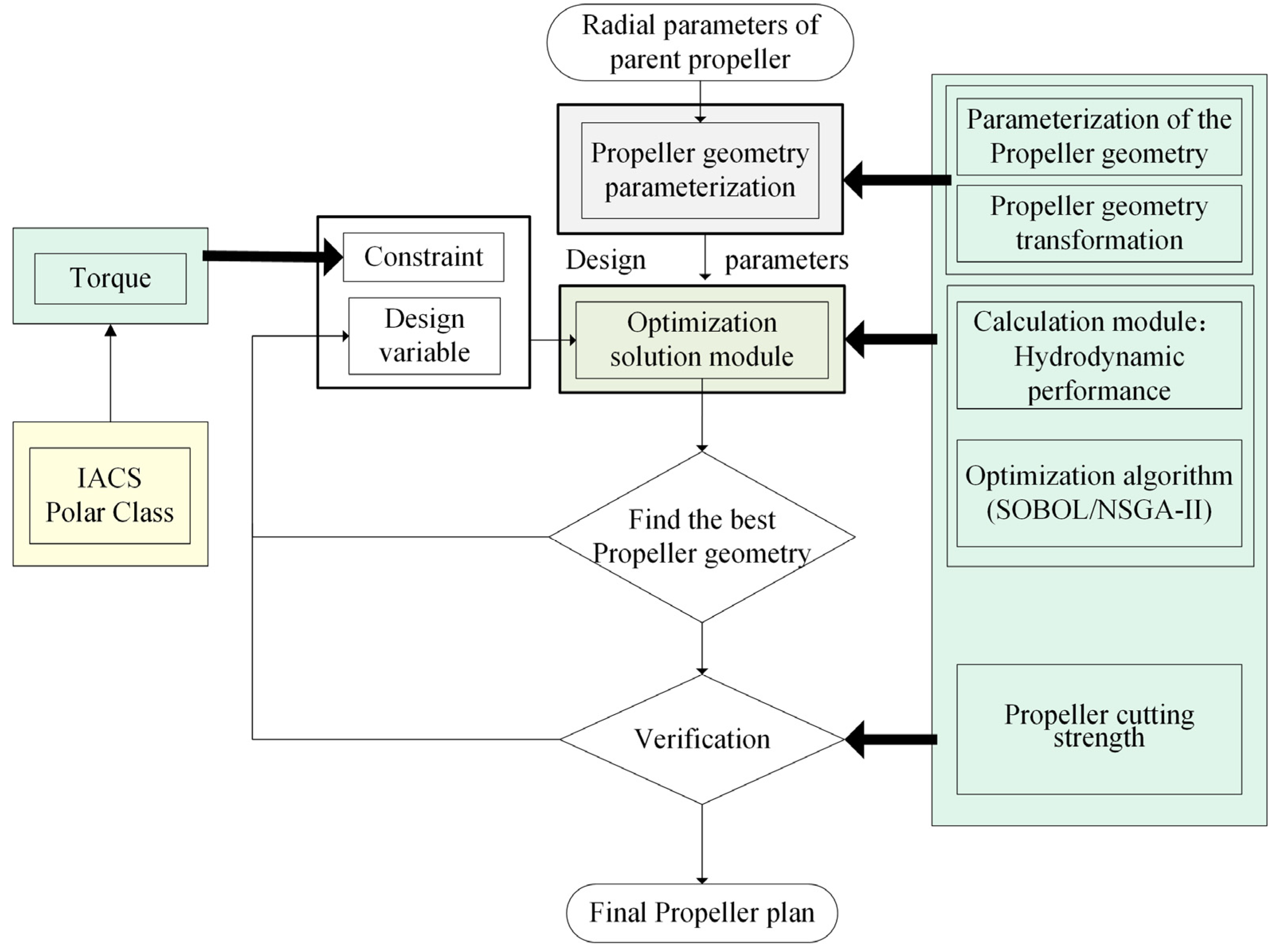
In this study, the ice propeller shape is to be optimized so that the hydrodynamic performance of the propeller can be improved, with the maximum ice torque as the optimization constraint under the condition that the ship’s shafting equipment remains unchanged during the optimization process. The propeller pitch, thickness, and camber at each radial direction are taken as the optimization design variables, and the optimization algorithm of SOBOL and NSGA-II is used.
Figure 5 is a flow chart of the propeller optimization design procedure. First, using the radial parameters of the propeller, the propeller geometric parameterization was modelled. Second, the CFD numerical calculation was performed to obtain the hydrodynamic performance, the thrust of the propeller coefficients and open water efficiency were taken as the design optimization goals. Third, the propeller shape is changed following the SOBOL algorithm and to perform a global uniform search, and then the NSGA-II algorithm was used to perform multi-objective optimization. The maximum torque
Qmax calculated by IACS Polar UR serves as the optimization constraint to make sure the toque from the deformed propeller cannot exceed the original propeller.
The pitch, thickness, and camber were used as design optimization variables, and the geometric model of the propeller was changed through the change of the pitch curve and the thickness curve. In this way, iteration was carried out to get the optimal propeller type scheme which can have best hydrodynamic performance.
6. Simulation of Ice–Propeller Interaction
This paper adopts a method based on explicit dynamics and uses SPH particles to simulate the phenomenon of ice being cut by propeller. Explicit dynamics applies explicit algorithms to dynamic equations. The biggest advantage of explicit algorithms is that they have better stability. The explicit dynamic equations use the central difference method, instead of solving the large-scale stiffness matrix like the implicit method, but include the nonlinear problem in the internal force vector of the equation. Generally, there is no need to perform balance iteration and the time step should be sufficient. Generally, there is no convergence problem. Compared with the implicit algorithm, the computational cost of the explicit algorithm is less than that of the implicit algorithm.
Anghileri et al. [
16] used three different methods (Lagrange (Lagrange), ALE (Arbitrary Langrangian-Euler), and SPH (Smooth Particle Hydrodynamics)) to numerically simulate the impact of hail on aluminum plates. For comparison, Pernas [
17] used the experimental model of Carney et al. [
18] to compare with the numerical results by the 3 methods in [
16]. The above studies have found that the simulation results based on the SPH method are more accurate to the experimental results than the Lagrange and ALE methods, and the calculation efficiency is higher, while the extreme large deformation of the structure can be more realistically simulated. The SPH method is a prominent mesh-free numerical method. Its advantage is that it is a pure Lagrange method, which can avoid the problems of mesh winding, distortion, and negative volume in the high-dimensional mesh method. It also avoids the shortcomings of the ALE method of constantly reconstructing the grid and increasing the calculation time, so it is suitable for the simulation of large dynamic deformation of ice in the ice–propeller collision problem.
6.1. Explicit Dynamics
Explicit dynamics is based on dynamic equations and is mainly used to calculate and solve the collision of three-dimensional inelastic structures and the dynamic response of deformation under impact. It is widely used in the engineering field. Impact is the process in which a projectile strikes a target at a certain speed, and at the same time, the energy is rapidly transformed in a relatively short period of time. The impact action can impose a high-intensity load on the target in a very short time, which in turn causes the movement of the target structure and even the destruction of the material. Explicit dynamics is a commonly used method to solve the impact and collision problem and its solution method uses the central difference method for calculation. The acceleration at time
t is:
Formula:
is the combined force vector of the external force applied;
is the internal force vector. The calculation formula is as follows:
,
,
are the equivalent nodes of the element stress field at the current moment, the hourglass resistance, and the contact force vector.
The speed and displacement of the node are obtained by the following formula:
The new geometric configuration is obtained by superimposing the initial position and the displacement increment:
In order to ensure the convergence of the entire calculation, when setting the time step, smaller time steps are often used, and the step length is set as follows:
is the highest natural frequency of the system, which is obtained from the eigenvalue equation of the smallest unit of the system:
6.2. SPH Particle Simulation
The SPH method is a meshless method based on the principle of interpolation, that is, a continuous object is discretized into movable particles with the same physical properties as the object, and each particle interacts through an interpolation function. The macro variables in SPH, such as temperature and density, can be calculated by converting the disordered point value into an integral interpolation form [
19]. The estimated value of each particle can be obtained through the interpolation function, and then the differential form is converted to the integral form through the dynamics of continuum, and then the mechanical behavior of the entire system can be obtained [
20]. The particle approximation function is:
W is the smooth function (or kernel function),
x is the position vector of any point,
y is the position vector of the approximate calculation point,
h is the smooth length, and
f is the function of the three-dimensional coordinate vector
x.
Smooth function
W is represented by auxiliary function
θ:
d is the spatial function.
Auxiliary function
θ is a cubic B-spline function, and its function is defined as:
C is the normalization constant, which is determined by the dimension of the space.
6.3. Material Model of Ice
In the simulation process of ice blade cutting, the accurate selection of the ice material model directly affects the accuracy of the results. Comparing with water, the inherent properties of sea ice are very complex, so a typical isotropic elastic fracture material is often used in numerical simulations. The relevant parameters of ice extraction in this paper are as in
Table 5 and
Table 6 [
21]:
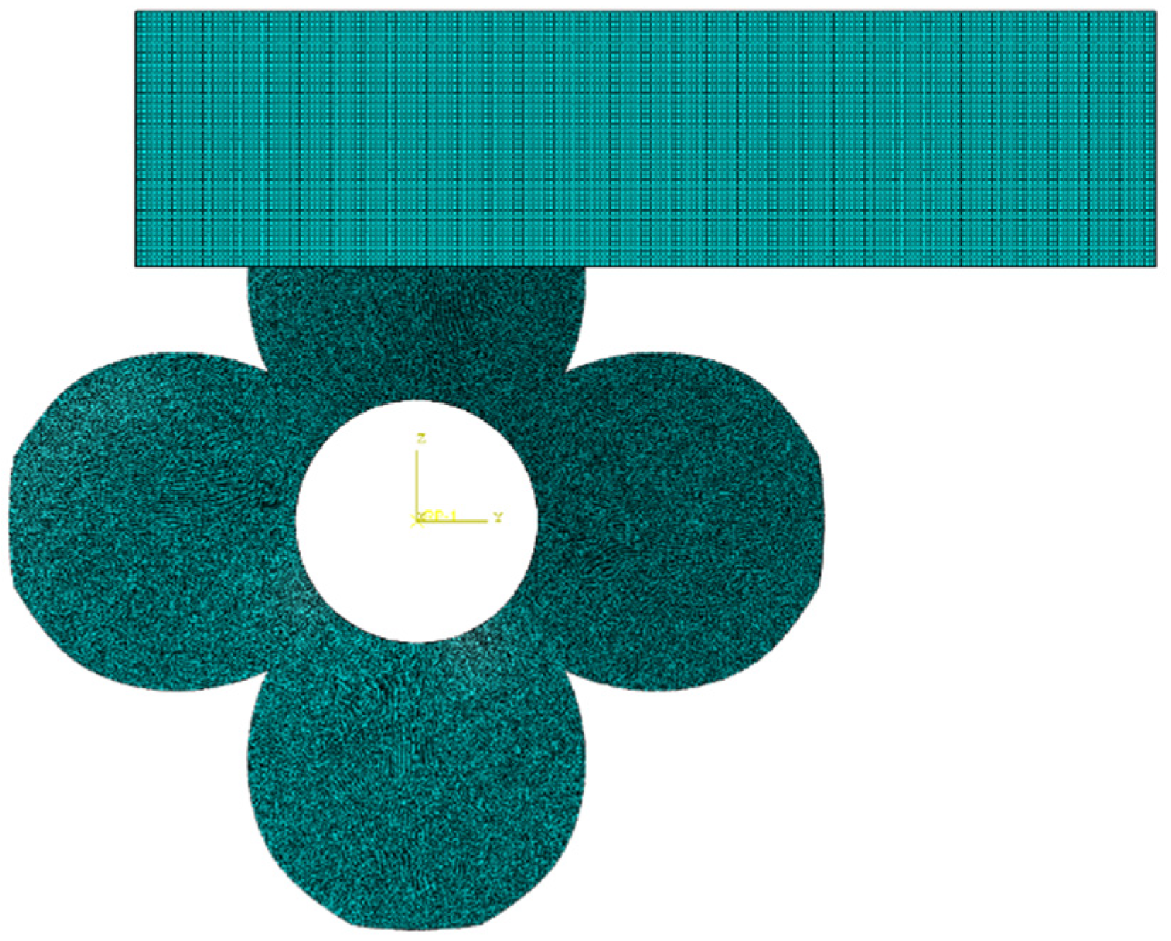
The ice cube model is a cuboid, L = 2 m, W = 2 m, D = 0.5 m. The relative position of the ice propeller is shown in
Figure 6:
7. Results
A sample ice propeller (PP0000C0) was selected as parent propeller for optimization following the procedure described in
Section 5 (
Figure 5). The optimized propeller with the best hydrodynamic performance was achieved while maintaining the maximum ice torque requirement based on IACS Polar UR (Equations (5) and (6)).
7.1. Propeller Hydrodynamic Performance
Using the above-mentioned pitch curve, thickness curve, and camber curve as design optimization variables, the propeller was globally optimized with multiple objectives at the design advance speed J = 0.4. The optimization goal was the open water efficiency and thrust coefficient of the propeller. The constraint condition was that the maximum torque caused by the optimized propeller to the shafting was less than that by the parent propeller. The NSGA-II algorithm was used for multi-objective optimization. Iteration was used to get the optimal propeller type scheme.
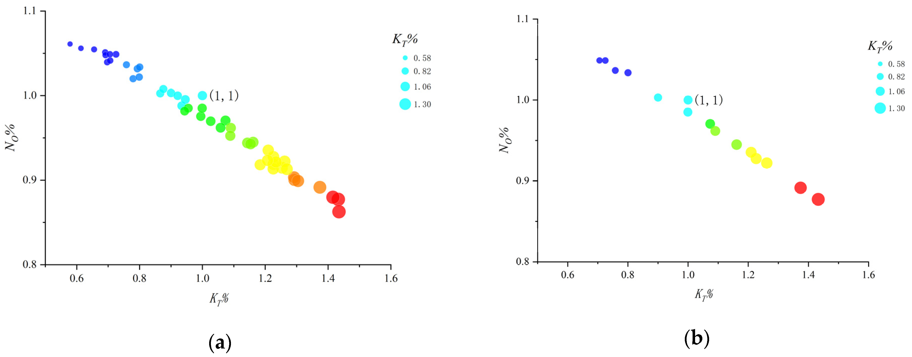
Figure 7 are the comparison of hydrodynamic performance of deformed propellers comparing to those of the parent propeller, in which, the
y-axis represents the ratio of open-water efficiency of deformed propeller to that of the parent propeller, the
x-axis represents the ratio of thrust coefficients of the deformed propellers to that of the parent propellers, and the coordinate point (1,1) in
Figure 7 is the parent propeller data point. The color of the bubble represents the open water efficiency and the diameter represents the thrust coefficient.
SOBOL was used to randomly search 50 individuals as shown in
Figure 7a, among which the best individuals were selected as shown in
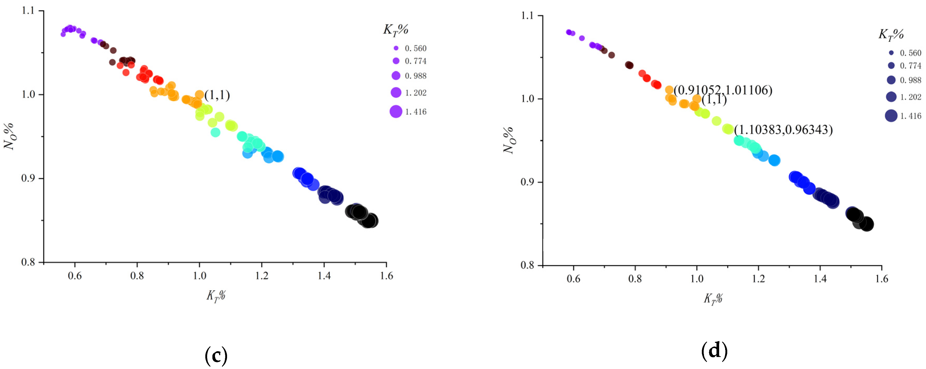
Figure 7b, and then NSGA-II algorithm optimization was performed based on the best individuals from SOBOL search. The population size during the optimization process was 10, a total of 20 iterations were performed, and 200 individuals were generated as shown in
Figure 7c. Then, we selected the better individuals from them for analysis as shown in
Figure 7d. It can be seen from the figure that the Pareto solution set is evenly distributed on the Pareto frontier.
Figure 7d are the ones selected through optimization. The torque from these optimized propellers are calculated according to IACS Polar UR and is smaller than that of the parent propeller. The propellers with higher efficiency and higher thrust coefficient (2 data points shown in
Figure 7d) were selected from them for the CFD calculation of full advancement speed.
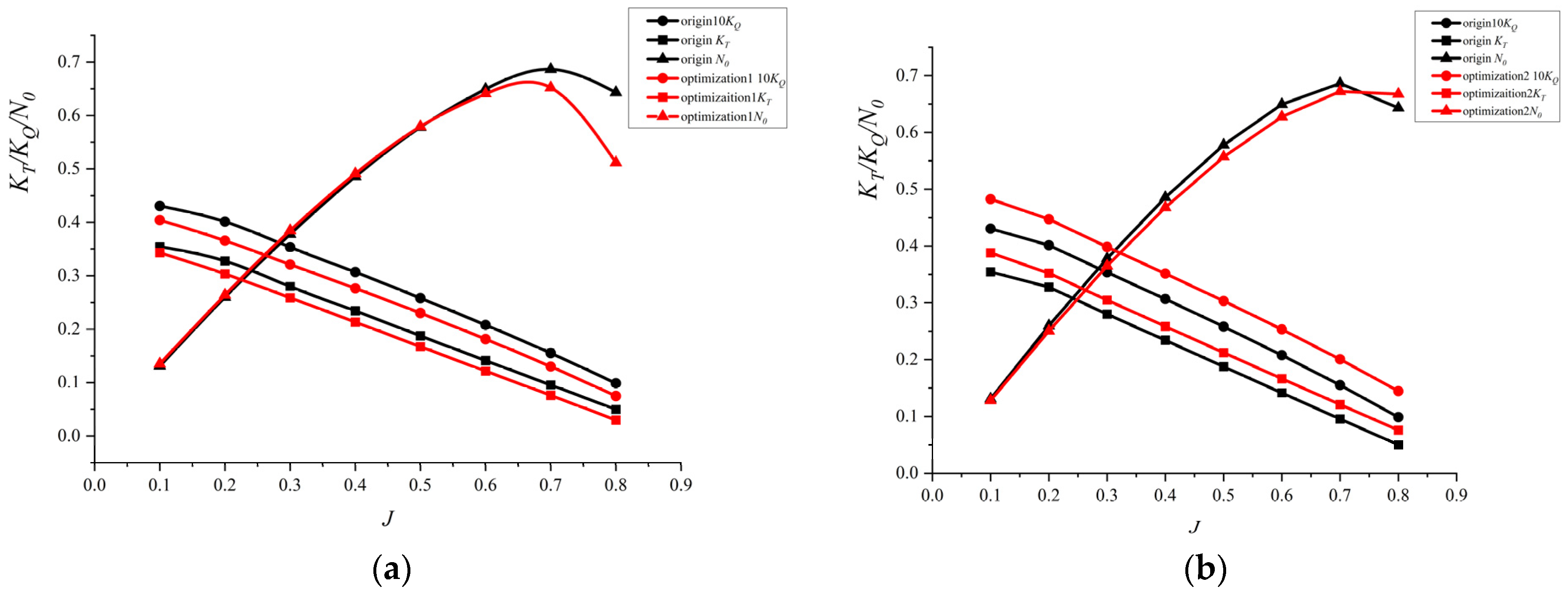
Through the CFD calculation of the optimized propeller, the open water curve comparison of the optimized propeller 1, the optimized propeller 2, and the parent ship is shown in
Figure 8a,b, and it is verified that the optimized propeller 1 and 2 meet the torque requirements by the IACS Polar UR specifications as shown in
Table 7. It can be seen from the comparison chart that the open water efficiency of the optimized propeller 1 is higher than that of the parent propeller at most advance speeds, and the torque is reduced by 25.69%, but the
KT and
KQ are lower than the parent propeller. The
KT and
KQ of the optimized propeller 2 are larger than those of the parent propeller, and the torque is reduced by 23.81%, but its open water efficiency is lower than that of the mother propeller.
CFD analysis are performed under the condition of
J = 0.4 for the selected optimized propellers and compared with the results of the parent propeller. As shown in
Table 8, the optimized 1 propeller has higher efficiency. It can be seen that
KT and
KQ are slightly reduced and the efficiency is improved. Optimized 2 propeller is the one with better thrust coefficient,
KT and
KQ are improved, and the efficiency is slightly reduced.
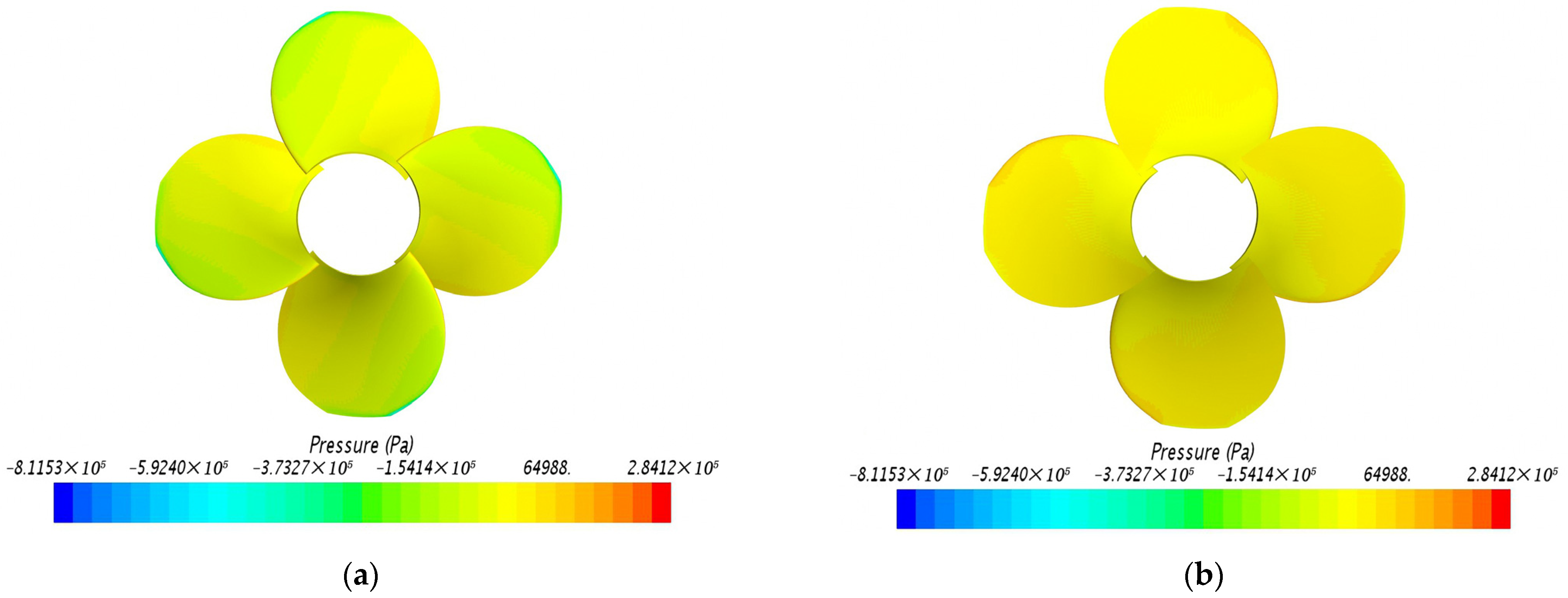
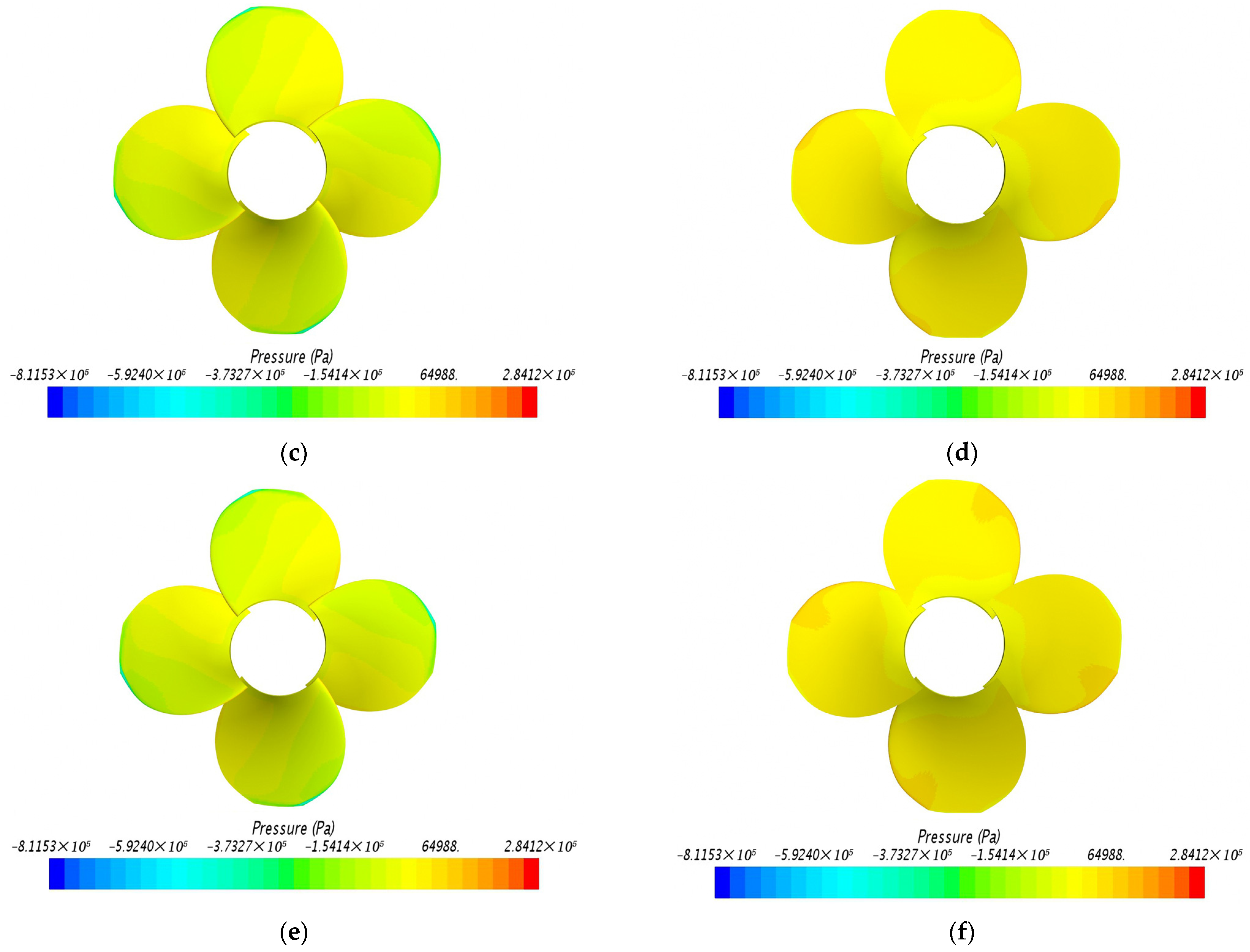
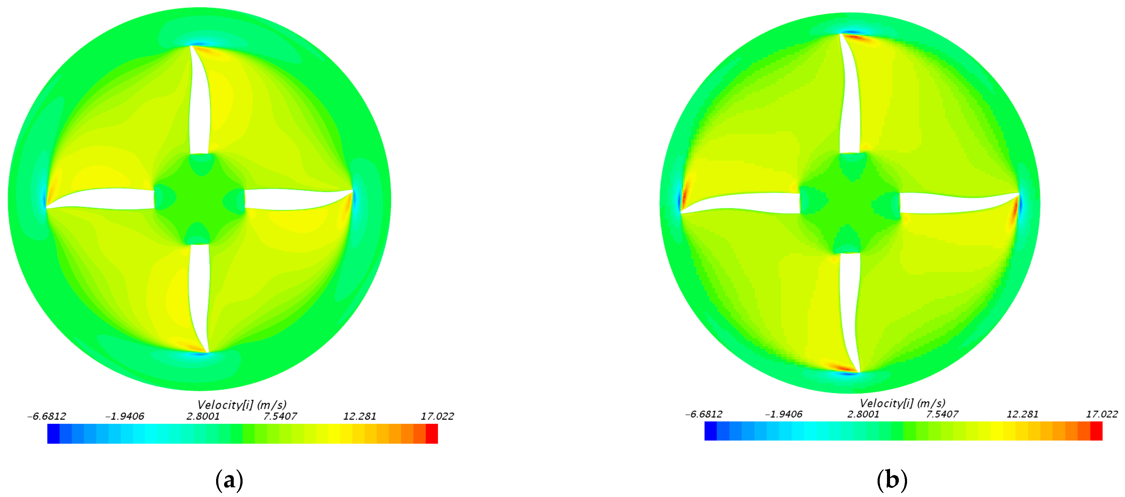
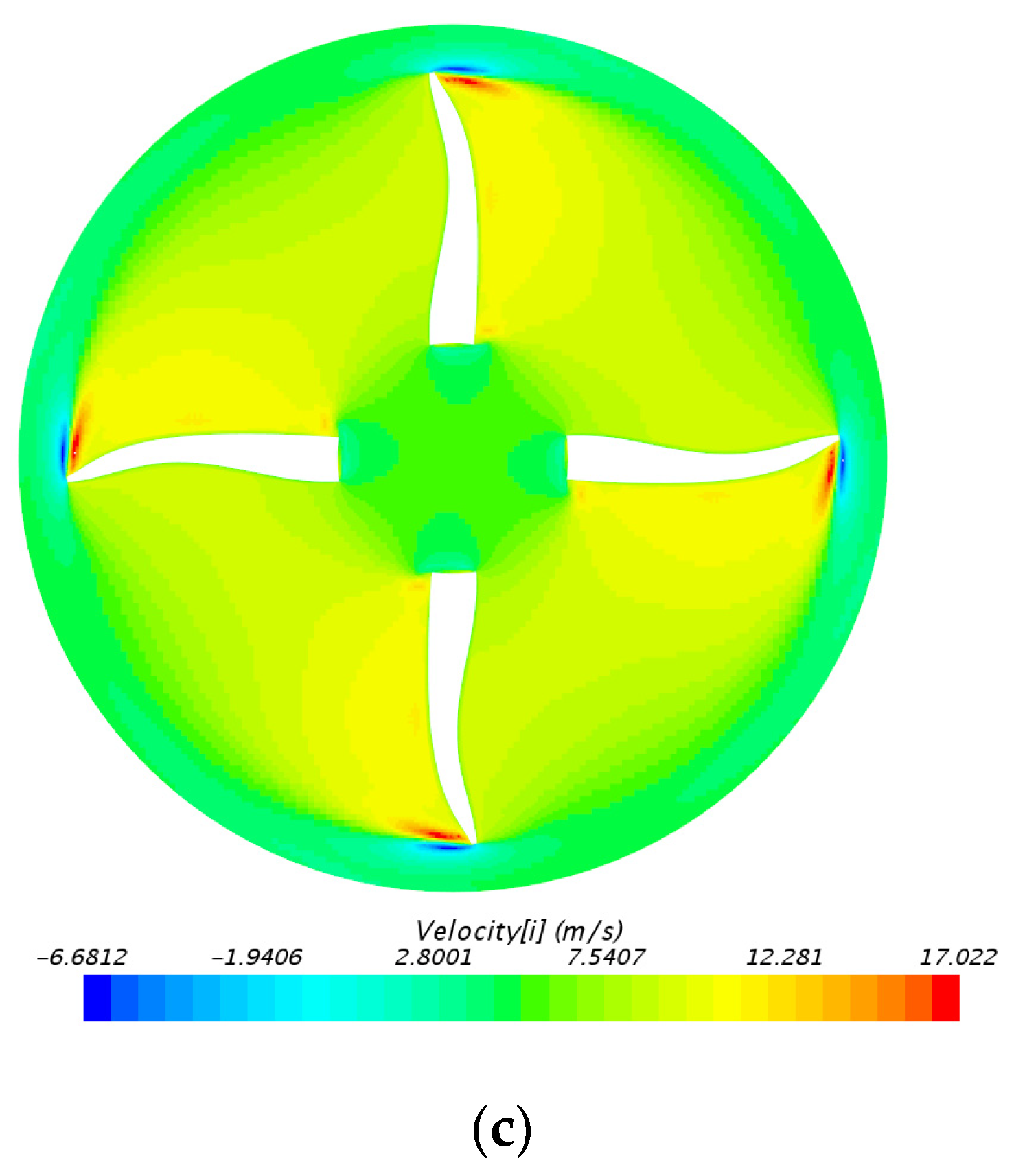
Figure 9 and
Figure 10 show the comparison of the back and surface pressure of the parent propeller and the optimized propeller under
J = 0.4 and the comparison of the axial speed at the disc surface. The thrust surface of the propeller is defined as the blade front, and the suction surface is defined as the blade back. Blade front pressure is positive and blade back pressure is negative. The pressure on the blade front is greater than the trailing edge, and the high-pressure area is concentrated near the leading edge and decreases gradually from the leading edge to the trailing edge; the pressure on the back of the blade shows a negative value, which is less than the trailing edge. Under the same advance speed coefficient, as the pitch ratio of the optimized propeller 1 decreases, the positive pressure on the blade front gradually increases and the negative pressure at the blade back gradually increases. The pressure difference between the blade front and the blade back of the propeller decreases as the pitch angle reduces; therefore, the thrust generated by the propeller decreases. With the increase of the pitch ratio of the optimized propeller 2, the positive pressure on the blade surface gradually increases and the negative pressure at the blade back gradually increases. In the case of high pitch ratio, local negative pressure increases near the leading edge of the blade back surface. In this case, the force on the surface of the propeller increases and cavitation is prone to occur. The pressure difference increases between the blade surface and the blade back of the propeller, that is, the thrust generated by the propeller increases, as the pitch angle increases.
From the velocity cloud map of the propeller disk surface, it was found that when the pitch is relatively low, and the area of the high-speed zone is relatively small. With the increase of the pitch ratio, the area of the high-speed zone increases and the area of the high-speed zone increases.
7.2. Strength Verification of Optimized Propellers
This paper uses the method of explicit dynamics to verify the strength and anti-icing performance of the propeller. First, we used the parent propeller, optimize propeller 1, and optimize propeller 2 to compare the stress on the surface of the propeller at the same speed. In the process of ice cutting, the force of propeller blades under actual conditions was simulated, which lays the foundation for subsequent research.
There are two problems in the numerical simulation of ice propeller cutting conditions based on actual conditions: (1) In actual sea conditions, the ice blocks are very irregular, which brings great difficulties to the modeling of ice blocks, and it is difficult to separate the ice blocks. (2) The influence of the hull structure is not considered, only the ice propeller contact model is established. Once the ice block contacts the propeller, the ice block may move away from the propeller without restriction, making it difficult to form a continuous cutting process.
In order to study the ice propeller cutting process, some simplifications need to be made to the ice propeller cutting model. For the propeller, its center point should be set as the reference point, rotating around the propeller axis at a certain speed. For ice cubes, it can be simplified into regular shapes as needed, such as spheres, cubes, etc. At the initial moment, all sea ice material points approach the propeller at the same speed. In order to enable the propeller to continuously cut the ice block, the upper end of the ice block can be constrained to move so that it moves at the same speed as the initial moment during the entire calculation process. Considering that the ice propeller contacting ice load is much larger than other loads, the influence of gravity, frictional resistance, and ice propeller interference with the hydrodynamic load are ignored in the calculation.
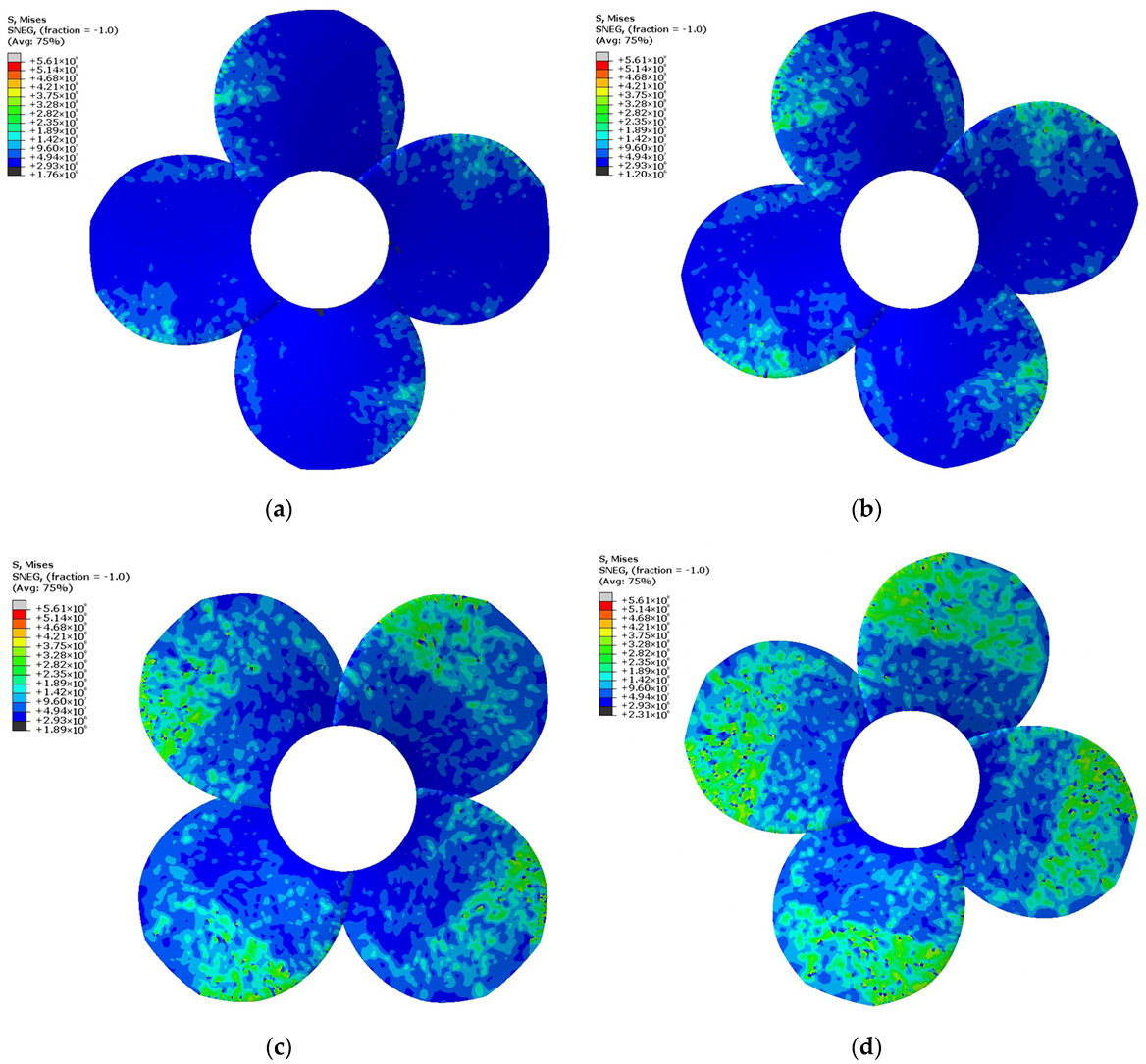
The stress cloud diagram at different stages of the blade is shown in
Figure 11. Numerical calculation results show that the maximum stress area of the blade under cutting conditions is mostly in the shadow area where cutting occurs with sea ice. It can be seen from the change trend of the pressure surface stress distribution of the blade in
Figure 11 that the blade tip is close to the leading edge after the ice blade starts to contact, that is, stress concentration occurs near the contact point. As time goes by, the blade continues to rotate and the contact area between the blade and the sea ice also has local deformation. The contact area gradually shifts from the leading edge to the following side, and the maximum stress distribution area of the blade also occurs, moving and staying near the lighted area where the propeller is in contact with the sea ice. The stress of the propeller blade during the ice blade cutting process is mainly concentrated in the area near the blade tip and leading edge. The cutting process is divided into three stages. The first stage blade stress is the largest, which is in line with the actual situation. With the continuous rotation of the blade, the stress concentration area gradually moves from the leading edge side of the blade tip to the following edge side, and the maximum stress coverage area during the entire contact process is mainly concentrated near the blade tip.
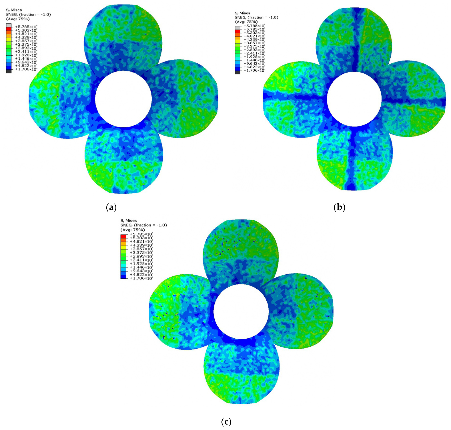
Then,
Figure 12 compared the parent propeller, optimized propeller 1, and optimized propeller 2 on the blade surface stress during the ice cutting process. After comparison, it was found that the stress at the tmaximum thickness of the optimized propeller 1 is significantly reduced because the thickness of the optimized propeller 1 is increased during the optimization process. The maximum surface stress of the optimized propeller 2 is lower than that of the parent propeller during the rotation. The surface stress of the optimized propeller does not exceed the allowable stress of the material. It shows that the optimization of this study is reasonable. Therefore, both the optimized propeller 1 and the optimized propeller 2 can be selected in this paper, which mainly depends on the user’s purpose. The designers can use the more efficient optimized propeller 1 or choose the optimized propeller 2 with a larger thrust coefficient.
7.3. Simulation of Ice and Propeller Cutting Process
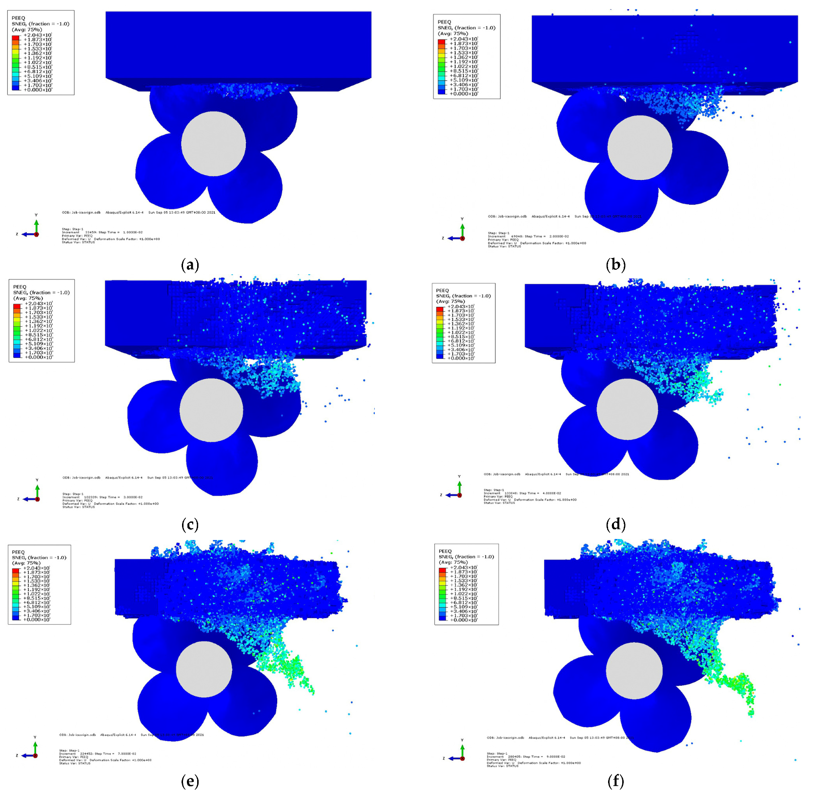
Figure 13 shows the destruction of sea ice during one revolution of the propeller under the condition of ice propeller cutting. The color in the figure represents the damage level of the bond, blue represents the ice material point in an intact state, and red represents the ice material point completely broken.
Figure 13a shows the process of cutting ice with the first blade. It can be seen from the color depth of the ice particles that the damage of the ice particles by the particles after the propeller is significantly increased. Because the initial cutting depth of the first blade is small, the resulting ice has a high degree of fragmentation, and the size of the resulting broken ice cubes is small. In the process of ice propeller cutting, the ice block has a forward movement speed, so the depth of the second blade cutting ice block in
Figure 13b is obviously increased. The cut ice block is relatively complete and relatively large, as shown in
Figure 13c, d. After the third blade, the cutting process of the ice propeller is basically stable, showing periodic cutting. The depth of cut and the size of the crushed ice formed during the cutting process of different blades are similar, as shown in
Figure 13e, f. In general, the ice cubes will form grooves after being cut by the propeller. Each time the propeller blades are cutting the ice, the depth of the grooves will increase. Due to the large randomness in the formation of ice cracks in the ice propeller cutting process, the shape of the broken ice is also greatly randomized. This is affected by many factors such as the shape and operating speed of the propeller, the characteristics of the propeller, and the characteristics of the sea ice itself. The broken ice will be accelerated by the cutting action of the propeller and will be thrown by the blades behind the cutting blade at a high speed. It is likely to hit the stern structure of the hull, causing ice-induced vibration of the hull or instantaneous high stress on the bottom of the ship, which has a great impact on the ship structure. The design and research and development of ships in ice areas requires special attention to this point.
8. Discussion
In this paper, a three-dimensional model of ice-class propeller is established by means of fully parametric modeling. A procedure to optimize the ice propeller shape is proposed and tested with a sample ice propeller. The objective of this optimization procedure is to improve the hydrodynamic performance of the propeller, with the maximum ice torque as the optimization constraint under the condition that the ship’s shafting equipment remains unchanged during the optimization process. The propeller pitch, thickness, and camber at each radial direction are taken as the optimization design variables, and the optimization algorithm of SOBOL and NSGA-II is used.
During the propeller optimization process, the multi-objective optimization of the hydrodynamic performance of ice-class propellers is carried out. Using the multi-objective optimization algorithm, this paper first selects the praetor front of the sample set as the optimal solution, and then selects the solutions with higher open water efficiency and the solutions with higher thrust coefficient from the pareto optimal solution as optimized targets, and use these optimized propellers to perform the hydrodynamic performance verification. It can be seen that the propeller with higher open-water efficiency has a decrease in propulsion coefficient and torque coefficient, while the open-water efficiency of propeller with higher propulsion coefficient has decreased, and the torque coefficient has increased.
This paper uses the method of explicit dynamics to check the strength of the propeller, and simulates the propeller ice cutting. The pressure distributions on the surface of the propeller blade are obtained, and the results show that the strength of the optimized propeller meets the requirements as the parent propeller. SPH particle method was used to simulate the ice state during the cutting process of the propeller and the ice, and the movement process of the ice particles were studied.
This following conclusions can be drawn from this study:
(A) The parametric modeling method used can control the pitch, camber, and thickness of the propeller, which can create variable blade section expression sand is beneficial to propeller blade design for improving the efficiency and thrust coefficient.
(B) The proposed fully parameterized method and multi-objective optimization procedure are proved to be valid for propeller design to improve the open water performance of ice propellers.
(C) Explicit dynamics model and SPH method can simulate the cutting process of propellers and ice, and well represent the movement process of ice particles after the ice broken by propeller blades.
Author Contributions
Conceptualization, Y.L. and S.L.; methodology, Y.L. and S.L.; software, C.W., Z.G. and C.L.; validation, Y.L. and S.L.; formal analysis, C.W, W.S. and C.L.; investigation, C.W., W.S. and C.L.; resources, S.L., Y.L.; data curation, C.W.; Writing—original draft preparation, Y.L. and C.W.; writing—review and editing, S.L.; visualization, C.W.; supervision, S.L. and Y.L.; project administration, S.L. and Y.L. All authors have read and agreed to the published version of the manuscript.
Funding
This work was funded by the National Natural Science Foundation of China Youth Project (Grant No. 51809029), the National Natural Science Foundation of China General Program Project (Grant No. 52171293), the Ph.D. Scientific Research Fund of the Natural Science Foundation of Liaoning Province (Grant NO. 2019-BS-025), the High-Level Talent Innovation Support Program of Dalian (Grant NO. 2020RQ009), the Key discipline project of Dalian Science and Technology Innovation Fund (Grant No. 2020JJ25CY016), the Fundamental Research Funds for the Central Universities (Grant No. 3132019306), Research Foundation for Talented Scholars (Grant No.00253015).
Institutional Review Board Statement
Not applicable.
Informed Consent Statement
Not applicable.
Data Availability Statement
The data presented in this study are available in this article (tables and figures).
Conflicts of Interest
The authors declare no conflict of interest.
References
- Chang, X.; Wang, X.D.; Wang, C.; Sun, S.X. Calculation and analysis of propeller strength under ice milling. J. Harbin Eng. Univ. 2017, 38, 1702–1708. (In Chinese) [Google Scholar]
- Searle, S.; Veitch, B.; Bose, N.; Reed, A.; Wilson, M.B.; Karafiath, G.; Morgan, W.B. HutchisonIce-class propeller performance in extreme conditions. Discussion. Authors’ closure. Trans. Soc. Nav. Archit. Mar. Eng. 1999, 107, 127–152. [Google Scholar]
- Moores, C.; Veitch, B.; Bose, N.; Jones, S.J. Multi-component blade load measurements on a propeller in ice. Trans. Soc. Nav. Archit. Mar. Eng. 2003, 110, 169–187. [Google Scholar]
- Wang, J.; Akinturk, A.; Bose, N. Numerical Prediction of Model Podded Propeller-Ice Interaction Loads. In Proceedings of the International Conference on Offshore Mechanics and Arctic Engineering, Hamburg, Germany, 4–9 June 2006. [Google Scholar]
- Wang, J.; Akinturk, A.; Bose, N. Numerical prediction of propeller performance during propeller-ice interaction. Mar. Technol. Sname News 2009, 46, 123–139. [Google Scholar] [CrossRef]
- He, F. Research on Calculation Method of Icebreaking Load and Icebreaking Capacity of Icebreaker; Harbin Engineering University: Harbin, China, 2011. (In Chinese) [Google Scholar]
- Hu, Z.; Gui, H.; Xia, P.; Wang, J. Finite element analysis of ship propeller strength under ice load. Ship Eng. 2013, 35, 12–15. (In Chinese) [Google Scholar]
- Guo, C.; Xie, C.; Zhao, D. Review of research on hydrodynamic performance of ice-class propellers. Ship Ocean Eng. 2014, 43, 1–8. (In Chinese) [Google Scholar]
- IACS. Requirements Concerning Polar Class; International Association of Classification Societies: Hamburg, Germany, 2019. [Google Scholar]
- Yin, H.; Lian, Q.; Zhao, Z.; Xu, Z. Development and Application of Model System for Optimization and Regulation of Drainage Network Based on Sobol Algorithm. In Proceedings of the 29th National Hydrodynamics Symposium, Zhenjiang, China, 24–25 August 2018. (In Chinese). [Google Scholar]
- Zhou, S.; Feng, Y.; Zhang, K.; Shen, S. Research on optimization of multi-effect evaporative seawater desalination system based on NSGA-II. Therm. Sci. Technol. 2021, 20, 112–121. (In Chinese) [Google Scholar]
- Liu, P.; Islam, M.F.; Searle, S.; MacNeil, A.; Prior, A. Design and Optimization of an Ice Class Propeller under Shallow Water, Semi-Tunnel Hull and Heavy Load Conditions. In Proceedings of the International Conference on Offshore Mechanics and Arctic Engineering, Hamburg, Germany, 4–9 June 2006. [Google Scholar]
- Zhou, Y. Research on Multi-Objective Optimization of Propeller Based on CFD Method; Wuhan University of Technology: Wuhan, China, 2016. [Google Scholar]
- Wang, X. CFD-Based Performance Study of Large Skew Propellers; Dalian Maritime University: Dalian, China, 2020. [Google Scholar]
- Wang, Y. Research on Panel-Vortex Particle Coupling Algorithm for Propeller Hydrodynamic Performance and Flow Field Analysis; Northwestern Polytechnic University: Xi’an, China, 2017. (In Chinese) [Google Scholar]
- Anghileri, M.; Castelletti, L.-M.L.; Invernizzi, F.; Mascheroni, M. A survey of numerical models for hail impact analysis using explicit finite element codes. Int. J. Impact Eng. 2005, 31, 929–944. [Google Scholar] [CrossRef]
- Pernas-Sánchez, J.; Pedroche, D.; Varas, D.; Lopez, J.; Zaera, R. Numerical modeling of ice behavior under high velocity impacts. Int. J. Solids Struct. 2012, 49, 1919–1927. [Google Scholar] [CrossRef] [Green Version]
- Carney, K.S.; Benson, D.J.; DuBois, P.; Lee, R. A phenomenological high strain rate model with failure for ice. Int. J. Solids Struct. 2006, 43, 7820–7839. [Google Scholar] [CrossRef] [Green Version]
- Zhang, S. Smooth Particle Hydrodynamics (SPH) Method (Review). Comput. Phys. 1996, 2–14. (In Chinese) [Google Scholar]
- Guo, X.; Zhai, R.; Kang, R.; Jin, Z.; Guo, D. Study of the influence of tool rake angle in ductile machining of optical quartz glass. Int. J. Adv. Manuf. Technol. 2019, 104, 803–813. [Google Scholar] [CrossRef]
- Sun, W. Research on the Propeller Strength of Ships Sailing in Ice Regions; Harbin Engineering University: Harbin, China, 2016. (In Chinese) [Google Scholar]
Figure 1.
Schematic diagram of the pareto frontier distribution of two objective functions.
Figure 1.
Schematic diagram of the pareto frontier distribution of two objective functions.
Figure 2.
Propeller fully parametric model.
Figure 2.
Propeller fully parametric model.
Figure 3.
Calculation domain of propeller.
Figure 3.
Calculation domain of propeller.
Figure 4.
Propeller meshing diagram: (a) X section grid; (b) Y section grid.
Figure 4.
Propeller meshing diagram: (a) X section grid; (b) Y section grid.
Figure 5.
Flow chart of optimized design system.
Figure 5.
Flow chart of optimized design system.
Figure 6.
The relative position of the ice and the propeller.
Figure 6.
The relative position of the ice and the propeller.
Figure 7.
Pareto solution and distribution (a) SOBOL50 individual; (b) SOBOL best individual. (c) NSGA-II200 individual. (d) NSGA-II best individual.
Figure 7.
Pareto solution and distribution (a) SOBOL50 individual; (b) SOBOL best individual. (c) NSGA-II200 individual. (d) NSGA-II best individual.
Figure 8.
Comparison of open water performance curves between the parent propeller and the optimized propeller. (a) Comparison chart of parent propeller and optimized propeller 1; (b) comparison chart of parent propeller and optimized propeller 2.
Figure 8.
Comparison of open water performance curves between the parent propeller and the optimized propeller. (a) Comparison chart of parent propeller and optimized propeller 1; (b) comparison chart of parent propeller and optimized propeller 2.
Figure 9.
Pressure distribution at propeller surface. (a) Parent blade back pressure; (b) parent blade front pressure; (c) Optimization 1 blade back pressure; (d) Optimization 1 blade front pressure (e) Optimization 2 blade back pressure; (f) Optimization 2 blade front pressure.
Figure 9.
Pressure distribution at propeller surface. (a) Parent blade back pressure; (b) parent blade front pressure; (c) Optimization 1 blade back pressure; (d) Optimization 1 blade front pressure (e) Optimization 2 blade back pressure; (f) Optimization 2 blade front pressure.
Figure 10.
Axial velocity at propeller surface. (a) Axial velocity of parent blade; (b) Optimization 1 the axial velocity of blade; (c) optimization 2 blade axial velocity.
Figure 10.
Axial velocity at propeller surface. (a) Axial velocity of parent blade; (b) Optimization 1 the axial velocity of blade; (c) optimization 2 blade axial velocity.
Figure 11.
Stress distribution during propeller and ice cutting. (a) Stress distribution during 0.035 s propeller and ice cutting; (b) stress distribution during 0.04 s propeller and ice cutting; (c) stress distribution during 0.05 s propeller and ice cutting; (d) stress distribution during 0.06 s propeller and ice cutting.
Figure 12.
Comparison of the surface stress of the original propeller, the optimization 1 propeller, and the optimization 2 propeller during ice cutting. (a) Comparison of surface stress of parent propeller and ice cutting; (b) Optimization 1 comparison of surface stress between propeller and ice cutting; (c) Optimization 2 comparison of surface stress between propeller and ice cutting.
Figure 13.
Propeller and ice cutting state. (a) 0.01 s; (b) 0.02 s; (c) 0.03 s; (d) 0.04 s; (e) 0.07 s; (f) 0.09 s.
Figure 13.
Propeller and ice cutting state. (a) 0.01 s; (b) 0.02 s; (c) 0.03 s; (d) 0.04 s; (e) 0.07 s; (f) 0.09 s.
Table 1.
Ice class coefficient table.
Table 1.
Ice class coefficient table.
| Ice Class | Hice (m) | Sice | Sqice |
|---|
| PC1 | 4 | 1.2 | 1.15 |
| PC2 | 3.5 | 1.1 | 1.15 |
| PC3 | 3 | 1.1 | 1.15 |
| PC4 | 2.5 | 1.1 | 1.15 |
| PC5 | 2 | 1.1 | 1.15 |
| PC6 | 1.75 | 1 | 1 |
| PC7 | 1.5 | 1 | 1 |
Table 2.
Main parameters of propeller.
Table 2.
Main parameters of propeller.
| Parameter | Numerical Value |
|---|
| D (diameter) | 1.6 m |
| Number of leaves | 4 |
| Disk ratio | 0.7387 |
| Pitch ratio | 0.83 |
| Hub diameter ratio | 0.3 |
| Side bevel | 0 deg |
| Airfoil profile | Naca66Mod a = 0.8 |
Table 3.
Changes of hydrodynamic parameters using different grid sets.
Table 3.
Changes of hydrodynamic parameters using different grid sets.
| Number of Grids | CFD KT | Error | CFD 10 KQ | Error | CFD η | Error |
|---|
| 0.2496 | 1.886% | 0.4123 | 0.561% | 0.5778 | 1.191% |
| 0.2501 | 2.082% | 0.4125 | 0.610% | 0.5789 | 1.384% |
| 0.2494 | 1.796% | 0.4099 | −0.024% | 0.5808 | 1.716% |
| 0.2491 | 1.673% | 0.4086 | −0.341% | 0.5819 | 1.909% |
Table 4.
Error comparison of propeller hydrodynamic results for different J value.
Table 4.
Error comparison of propeller hydrodynamic results for different J value.
| J | Test Value KT | CFD KT | Error | Test Value KQ | CFD
KQ | Error | Test Value
η | CFD
η | Error |
|---|
| 0.5 | 0.285 | 0.294 | 3.123% | 0.0477 | 0.0465 | 2.413% | 0.475 | 0.502 | 5.68% |
| 0.6 | 0.245 | 0.248 | 1.22% | 0.041 | 0.0408 | −0.49% | 0.571 | 0.5809 | 1.73% |
| 0.7 | 0.2 | 0.205 | 2.50% | 0.036 | 0.0353 | −1.94% | 0.619 | 0.647 | 4.52% |
Table 5.
Material model of propeller.
Table 5.
Material model of propeller.
| Parameter | Numerical Value |
|---|
| Material | Nickel Aluminum Bronze |
| Elastic Modulus | 117 Gpa |
| Poisson’s ratio | 0.34 |
| Density | 7600 kg/m3 |
| Allowable stress | 620 Mpa |
Table 6.
Material model of ice.
Table 6.
Material model of ice.
| Density | Shear Modulus | Elastic Modulus | Poisson’s Ratio | Yield Stress | Bulk Modulus | Failure Strain | Cut-Off Pressure | Plastic Hardening Modulus |
|---|
| 900 kg/m3 | 2.2 Gpa | 6.312 Gpa | 0.3 | 2.12 Mpa | 5.26 Gpa | 0.35% | −4 Mpa | 4.26 Gpa |
Table 7.
Verification of ice torque by IACS Polar UR.
Table 7.
Verification of ice torque by IACS Polar UR.
| P7 | Hice (m) | Sice | Sqice |
|---|
| | 1.5 | 1 | 1 |
| | parent propeller | optimized propeller 1 | optimized propeller 2 |
| Qmax (kNm) | 22.9781 | 17.0747 | 17.5064 |
| Compared | 0% | −25.69% | −23.81% |
Table 8.
J = 0.4 performance comparison of open water.
Table 8.
J = 0.4 performance comparison of open water.
| | Parent Propeller | Optimized Propeller 1 | Compared | Optimized Propeller 2 | Compared |
|---|
| J | 0.4 | 0.4 | | 0.4 | |
| KT | 0.234 | 0.213 | −8.83% | 0.259 | 10.53% |
| 10 KQ | 0.307 | 0.276 | −9.85% | 0.352 | 14.69% |
| NO | 0.485 | 0.491 | 1.13% | 0.468 | −3.63% |
| Publisher’s Note: MDPI stays neutral with regard to jurisdictional claims in published maps and institutional affiliations. |
© 2021 by the authors. Licensee MDPI, Basel, Switzerland. This article is an open access article distributed under the terms and conditions of the Creative Commons Attribution (CC BY) license (https://creativecommons.org/licenses/by/4.0/).


