U.K. House Prices: Bubbles or Market Efficiency? Evidence from Regional Analysis

Abstract

This paper studies U.K. regional house prices across nine regions from January 2005 to December 2017 to identify regional versus national effects on house prices and potential house price bubbles. It uses a version of the Gordon dividend discount model, modelling house prices as the present value of imputed rents as a measure of fundamentals. It differentiates between long-term and short-term effect using pooled mean group (PMG) and mean group estimation (MG) to determine variations in regional house prices during different periods relating to the most recent financial crisis. The results confirm that the crisis had differentiating effects in the short term, but there is reversion back to long-run fundamentals. Regional trend analysis shows that the house price growth in the regions has been affected differently in the short run and each region has varying long-run fundamentals. Residential property values in London have shown strongest short-run momentum.

1. Introduction

Ten years after the global financial crisis (GFC) of 2008/2009, the U.K. housing market recovered and has been experiencing another boom period until 2017. This has resulted in an increasing debate regarding a new house price bubble and the impact on regional economies in the United Kingdom. The aim of this paper is to identify the reason for the most recent rises in house prices in the United Kingdom at the regional level and test whether or not a house price bubble does indeed exist within the regions. The analysis will identify if the most recent changes are part of a regime shift or the effect of a new short term residential housing bubble. For the purposes of this research, we define a bubble as the deviation of expected house price growth based on fundamentals from actual observed house price growth. Further, we define house price growth as a function of lagged responses to the present value of expected future cash flows (imputed rents).

First studies on property market bubbles started in the U.S. market. The property market in the United States during 1998–2008 has been widely perceived as having had a bubble, but with the interest rate decline during the 1990s and early 2000s, fundamental factors had also changed. An acceleration of house prices took place from 2000 to 2006. This coincides with the growths of the subprime mortgage market, securisation, and credit expansion. Credit market liberalization has also occurred in other countries, including the United Kingdom. Barrell et al. (2004) and the Organisation for Economic Co-operation and Development (OECD) (2005) suggest that U.K. house prices were overvalued by 30% or more during the period 2003–2004. However, the effects have not been studied in depths and the argument is split between those who argue in favour of a bubble and those who argue there was a fundamental regime shift. Nickell (2005), for example, rejects the bubble hypothesis based on the argument that a shift in fundamentals has occurred.

However, after the global financial crisis (GFC) and the collapse of credit markets and house prices, several countries have experienced increased house price growth due to excess cash availability globally. Some research has focused on foreign real estate investment and its impact on house prices and the economy. This has been a popular topic in different countries including Australia, China, Korea, Malaysia, Spain, Vietnam, and other countries (Gholipour et al. 2014; Rodríguez and Bustillo 2010; Rogers et al. 2015). Since the GFC, the United Kingdom in particular has been a safe haven for foreign investors. A lot of this capital has been focused on real estate investments, hence there is reason to believe that this has led to a new housing bubble. The assessment of the most recent house prices changes—including the question, if this represents a fundamental regime shift with regard to the role of real and nominal interest rates—is thus of wider interest.

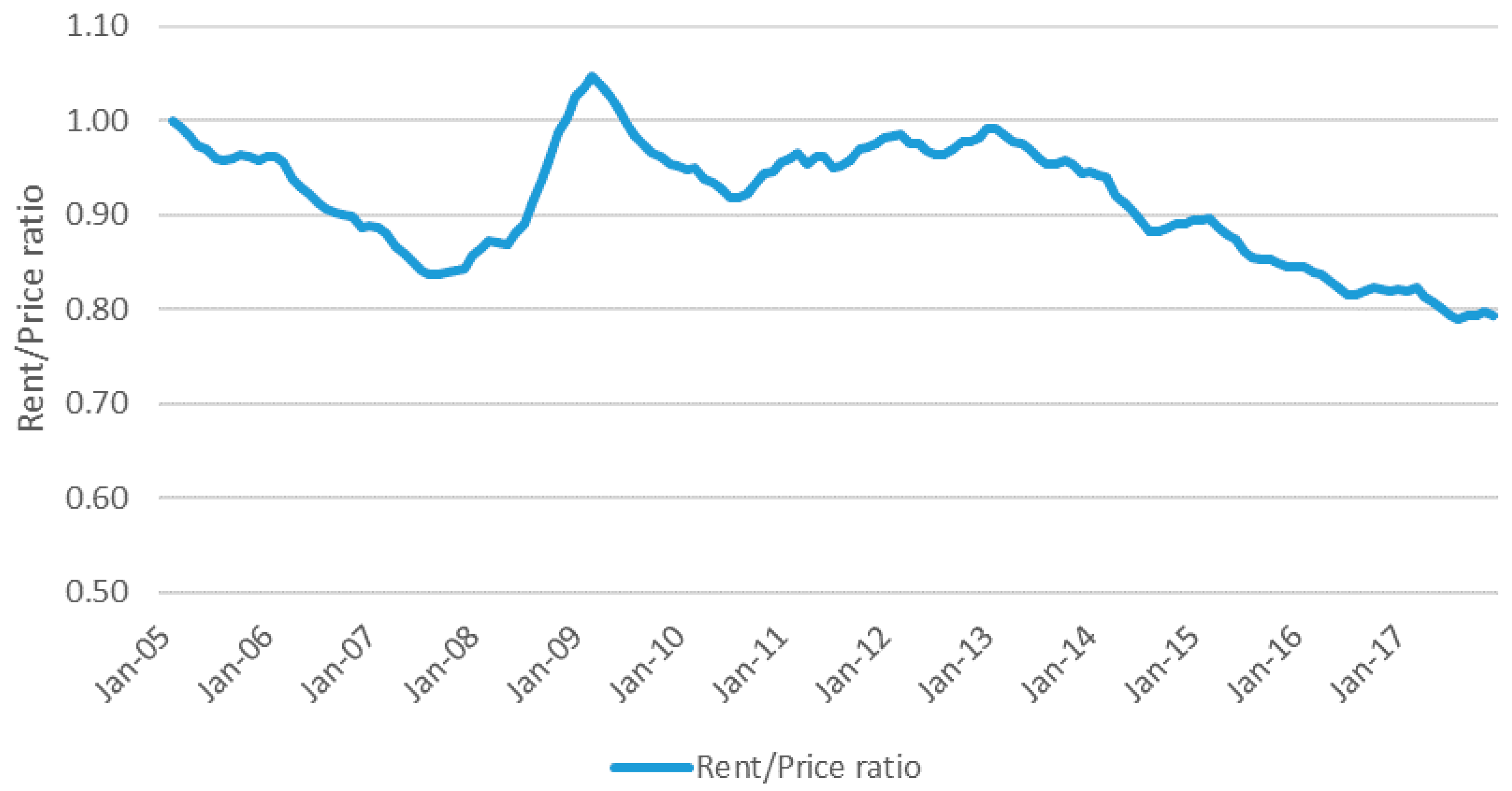
Figure 1 shows the development of house price growth and rental growth on national U.K. level in form of the rent to price ratio. The series shows that in fact, house price growth outpaced rental growth for most of the period on the national level. A potential house price bubble is visible during the years leading up to the financial crisis, when house price growth was higher than rental growth shown in the rent to price ratio below 1.

When house prices and selling activity reached a low point in 2009, rental growth was outpacing house price growth for a short period. Over the last five years, the graph shows the clear pickup in the pace of house price growth again, similar to the pre-crisis period. Overall U.K. national house prices increased by 30% compared with rent, which grew only by 17% between December 2007 and December 2017.

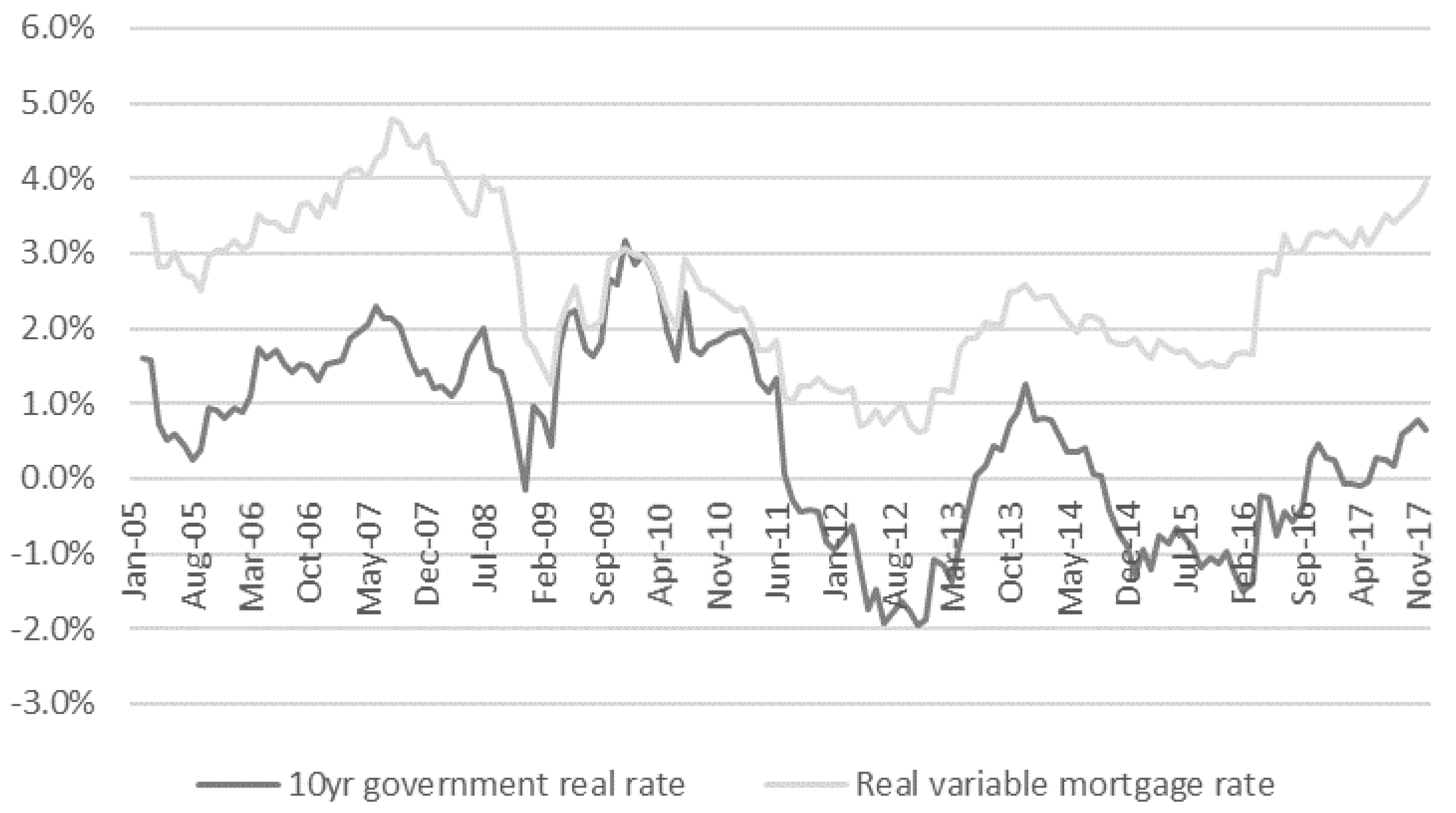
The second key variable to our model is interest rates. As the effect of inflation would distort our analysis of real price growth based on fundamentals, our analysis is based on real rates rather than nominal rates. Figure 2 shows the 10-year government real bond rate as a reference rate for long-term interest rates together with the variable mortgage (real) rate by Nationwide Building Society. As a result of higher inflation than interest rates observed from 2012 onwards, real interest rates in the United Kingdom have been negative for some periods and only recently returned to positive rates.

Thirdly, the paper also aims to explore the wider issues of house price increases, credit availability, and the effect on regional economies. The impact of housing market volatility has been widely discussed in the years following the onset of the banking crisis. Volatility especially affects certain pockets of the market characterised by chronic under-supply of new homes; stretched affordability; falling home ownership; and, in some areas, large-scale investment that some have described as speculative. We thus have tested the relevance of additional fundamental variables including regional disposable household income, first time buyer affordability, and price to earnings ratio, and found that price to earnings ratio was significant on national and regional level. Adding regional price to earnings ratio data as a local demand factor is one of the key contributions in this research.

Based on the Gordon dividend discount model, we study nine regions from January 2005 to December 2017. Our hypothesis is that different regions have different levels of “momentum”. Using mean group (MG) and pooled mean group (PMG) analysis confirms significant differences between long-term and short-term effects and differences in “momentum” within regions, namely London and the North East. The variable residential mortgage rate and regional earnings ratios are significant factors to determine rent to price ratio. Moreover, the regions do not share the same long-run equation, factors are specific to every region.

More generally, the research also explores the impact of credit availability and low interest rates and if these can be classified as change away from long-run fundamentals, resulting in short term effects that potentially lead to house price bubbles. Breaking down the period based on the financial crisis, we find that the variable residential mortgage rate significantly positively relates to rent to price ratio during the financial crisis in the long run, but negatively in the short run. At the same time, the 10-year government real bond rate had no significance during the period of the crisis, but shows significance again in the post-crisis period.

The following detailed analysis is structured into five sections. The next section provides a literature review of the previous studies, followed by the third section, which presents the basic modelling approach for house price growth with a description of the data employed. The fourth section presents an in-depth analysis of the results, followed by some additional discussion in the final section.

2. Literature Review

In spite of the widespread interest in real estate bubbles, the analytics of such paths remain largely unexplored. One main approach is to view asset bubbles as a rapid and unsustainable growth in asset prices that cannot be explained by “fundamental” factors. According to Stiglitz, the reason that the price is high today is only because investors believe that the selling price will be high tomorrow—when “fundamental” factors do not seem to justify such a price—then a bubble exists” (Stiglitz 1990).

A number of empirical tests have been developed to exploit the link between asset prices and various fundamental values. West (1987) proposes an empirical test for the existence of a bubble using the constant expected return model. His approach relies on comparing two sets of parameters. One set of estimates is obtained by a projection of stock prices based on past dividends, and the other is obtained by a set of equations describing the discount rate and the dividend process. This and other tests to identify bubbles are reviewed in Flood and Hodrick (1990). Meese and Wallace (1994) examine whether the real expected return on home ownership is close to the real homeowner cost of capital by studying the relationship between price, rent, and the cost of capital. Abraham and Hendershott (1993, 1996) study the relationship between house prices, construction costs, real income growth, and interest rates. They find that these factors explain half of the historical variation in house price appreciation. The bubble then manifests itself in the “sustained serially correlated deviations”, yet it remains unclear whether these deviations are because of a “bubble” or a misspecification of the econometric model. Himmelberg et al. (2005) compare the level of housing prices with local rent and income for a period of 25 years. They explain that changes in the price-to-rent and price-to-income ratios might suggest the existence of bubbles even when houses are reasonably priced, because they fail to account, for example, for differences in risk, property taxes, and maintenance expenses, and anticipated capital gains from owning a home. Glaeser et al. (2008) present a theoretical model of housing bubbles, which predicts that areas with more elastic supply will have fewer bubbles with shorter duration and smaller price run-ups. Their data indicate that the price increases in the 1980s were almost exclusively experienced in areas with inelastic supply.

Recent tests for speculative bubbles in regional U.S. housing markets typically consider deviations from market fundamentals. Goodman and Thibodeau (2008) explore to what extent house appreciation rates over the time period 2000–2005 can be attributed to economic fundamentals and what portion can be attributed to speculation. According to these authors, much of the appreciation is the result of inelastic supply and speculative motives are present in less than half of the cities they examined. Mikhed and Zemčík (2009) present a panel test to detect bubbles using price–rent ratios for the period 1975–2006. The bubble indicator they constructed detects bubbles around the decade turn in the late 1980s and the early 1990s, as well as around the end of the 1990s. Peláez (2012) argues that the housing bubble in the late 1990s and the early 2000s could have been predicted when considering the unprecedented growth rate of the house price to per capita income ratio.

Defining the relevant periods in which bubbles grow and collapse opens new avenues for future research on the impact of fundamentals on housing price movements both in and outside of the bubble periods. Lai and Van Order (2010, 2017) also find that different periods have to be tested. While they find that between 1999–2005, house prices are largely explained by fundamentals such as decline of long-term interest rates, the short period from 2003–2005 shows a price bubble associated with big changes in markets, such as securitization and sub-prime mortgages.

There is a rapidly growing strand in the recent literature on housing price dynamics that tries to identify the effects of various fundamental values on prices. Using simulation of the U.S. housing market, Khandani et al. (2013) find that the declining interest rates and the growth of the refinancing business contributed significantly to the recent housing boom and the massive defaults during the bust. Favilukis et al. (2017) argue that much of the housing price appreciation can be explained by relaxation of credit constraints, and Mayer and Sinai (2009) show that markets with the highest subprime lending experienced the greatest growth in price-to-rent ratios. In contrast, Glaeser et al. (2010) present evidence supporting the view that easy credit in the form of low real interest rates and permissive mortgage approval standards is not a strong contributor to the rising house prices. Differentiating from the previous studies, we incorporate earnings ratio as an additional regional fundamental variable to explain the various risk factors represented in the discount rate used in the Gordon dividend discount model. Further, we test the different levels of “momentum” and use mean group (MG) and pooled mean group (PMG) analysis to obtain the properties of short-run momentum and long-run mean reversion.

3. Methods and Materials

3.1. Basic Modelling of House Price Growth

For the current research, a house price bubble is defined as a change in the properties of deviations of actual house price growth from its fundamentals, which come from estimates of house price growth as a function of lagged responses to the present value of expected future rent. This allows for a parsimonious specification using only lagged property values, interest rates, and rent, which are summary statistics for all sorts of variables commonly used in modeling real estate to explain residential property values. Borrowing from Fama and French (1988) and Cutler et al. (1991), the logarithm of the market price of an asset is divided into (1), a nonstationary part that describes the fundamental price, and (2), a stationary component that implies the returns are predictable (from previous returns).

We use the Gordon dividend discount model to model house prices as expected present value of imputed rent, which is similar to the work on housing bubbles by Black et al. (2006), Hwang and Quigley (2006), Taipalus (2006), and Chan et al. (2001), as well as the pricing model by Glaeser and Nathanson (2017) for house prices, where traders are “almost” rational. The optimal forecasting procedure uses past prices to forecast future house prices in a way that allows short-run momentum to divert from the long-run, with long-run mean reversion and excess volatility. We add the restriction that the long-run mean is given by the Gordon dividend model.

Following the Lai and Van Order (2010, 2017) framework, we define the “fundamental” value as the price given an information set, $\mathsf{\Omega }$ where the transversality condition means that the second term approaches zero holds (Giglio et al. 2016). This gives the equilibrium condition for holding property at time $t$ as follows:

$$P_t={\displaystyle \sum _{i=0}^{\infty }E(}{R}_{t+i}/D_{t+i}^i|{\mathsf{\Omega }}_t)$$

(1)

where $P$ is the housing price; $R$ is the net rental income, in this case, imputed services of the property; and $D$ is the risk-adjusted discount factor. Dividing through by $R_t$, we have

$$P_t/R_t={\displaystyle \sum _{i=0}^{\infty }E(}(R_{t+i}/R_t/D_{t+i}^i|{\mathsf{\Omega }}_t)$$

(2)

which corresponds to a price earnings ratio for equities. However, for our further analysis, we use the reciprocal of this $P_t/R_t$, which is the rent-to price ratio, as the more commonly used variable in real estate markets.

Based on Equations (1) and (2), it is assumed that expected interest rates and future rents are correlated and the adjustment process can be expected to vary significantly across regions with different geography. The next expression (2) is approximated by the Gordon model used for pricing stocks, that is, if interest rates are constant and rents grow at a constant rate, rearranging the formula results in the following:

$$\frac{R_t}{P_t}={\alpha }_i{i}_t-{\alpha }_{\pi }{\pi }_t{}^{*}+\alpha \equiv {\gamma }_i{i}_t+{\gamma }_r{r}_t+\alpha$$

(3)

where $i$ is the interest rate; ${\pi }_t{}^{*}$ is the expected rate of rental growth; $r=(i_t-{\pi }^{*})$ is the real rate; and $\alpha$, ${\alpha }_i$, ${\alpha }_{\pi }$, ${\gamma }_i$, and ${\gamma }_r$ are parameters. In general, we expect ${\gamma }_r$ to be close to 1, ${\alpha }_i$ and ${\alpha }_{\pi }$ to be positive, and we are not sure about the sign of ${\gamma }_i$. Hence, testing for the magnitude of signs, especially for ${\gamma }_r$, requires calibrating our assumptions. We develop a model as expression (4) to simulate the long-run price estimates for every region, but allow long adjustments, which vary across regions. Furthermore, the Gordon model assumes a constant growth rate in perpetuity, which is not realistic. Adopting the Gordon model for the estimation of house prices, we added additional risk parameters such as the regional earnings ratio to allow for a variable discount rate. Further, to simplify the process, we assume there is no taxation on capital gains on housing, resulting in the following:

$$\frac{R_t}{P_t}=(1-t)i_t-{\pi }_t{}^{*}+\alpha \equiv -ti+r+\alpha$$

(4)

where $t$ is marginal tax rate meaning no difference between owning and renting, and $\alpha$ contains risk adjustments as well as depreciation and long-run expected future rental growth. The next step of the analysis is to reconstruct the model into the relationship of lagged long-run and short-run effects among variables using the pooled mean group (PMG) and mean group (MG) estimation models developed in (Pesaran and Smith 1995; Pesaran et al. 1997). This allows regional real estate data to have the properties of short-run momentum and long-run mean reversion. This means standard asset pricing theory can be applied in the long-run, while allowing for sluggishness of price adjustment and variation of adjustment speeds across different U.K. regions. The dynamic panel estimation model can be represented by the following:

$$\Delta \frac{R_{c,t}}{P_{ct}}={\displaystyle \sum _{j=1}^l{\lambda }_{c,j,}}\Delta \frac{R_{ct-j}}{P_{ct-j}}+{\displaystyle \sum _{j=0}^q{\displaystyle \sum _{k=1}^n{\delta }^k{}_{c,j}}{x}^k{}_{c,t-j}}+{\alpha }_c+{\epsilon }_{c,t}$$

(5)

where $\frac{R_{c,t}}{P_{ct}}$ is residential rent to price ratio in region $c$ at time $t$, $x^k{}_{c,t-j}$ is the kth of $n$ regressors for region $c$, and ${\alpha }_c$ captures region specific fixed effects. ${\epsilon }_{c,t}$ are the regions’ specific errors, c represents regions, $t$ represents time in month, and $j$ is an indicator of lags. When it is written in error correction form, this results in the MG estimation, where some of the parameters are restricted inside the brackets to be zero. Consequently, we obtain the following long-run specification (6).

$$\Delta \frac{R_{c,t}}{P_{ct}}={\varphi }_c\left\{\Delta \frac{R_{ct-j}}{P_{ct-j}}-{\displaystyle \sum _{k=1}^n{\beta }_c{}^k{x}_{c,t}^k}\right\}-{\displaystyle \sum _{j=0}^q{\displaystyle \sum _{k=1}^n{\delta }^k{}_{c,j}}△x^k{}_{c,t-j}}+{\alpha }_c+{\epsilon }_{c,t}$$

(6)

where

$${\varphi }_c=-(1-{\lambda }_c),{\alpha }_c=\frac{{\mu }_c}{(1-{\lambda }_c)},{\beta }_c=\frac{({\delta }_{1,c,j}+{\delta }_{2,c,j})}{(1-{\lambda }_c)}$$

If assuming homogeneous long-run relationships for the PMG estimation model, resulting in ${\beta }_c{}^k={\beta }^k$ for all regions, then Equation (6) can be written as follows:

$$\Delta \frac{R_{c,t}}{P_{ct}}={\varphi }_c\left\{\Delta \frac{R_{ct-j}}{P_{ct-j}}-{\displaystyle \sum _{k=1}^n{\beta }^k{x}_{c,t}^k}\right\}-{\displaystyle \sum _{j=0}^q{\displaystyle \sum _{k=1}^n{\delta }^k{}_{c,j}}△x^k{}_{c,t-j}}+{\alpha }_c+{\epsilon }_{c,t}$$

(7)

Finally, if PMG in Equation (7) is preferred to MG in Equation (6), then it can be inferred that all regions of concern share the same long-run effects, while allowing different regions to adjust at different rates and in different ways. Both Equations (6) and (7) allow us to restrict some of the parameters inside the brackets to be zero, so that the long-run specification that looks like the Gordon model, as given in Equation (3), but with fewer restrictions on short-run adjustment parameters across regions. Our expectation is that that the error correction coefficients ${\varphi }_c$ will be negative and the sums of the coefficients of lagged changes in $R/P$ (momentum) will be positive but less than 1 (in order that the model converge), which means that there is no bubble in this region. The residuals ${\epsilon }_{c,t}$ are assumed to follow the autoregressive process.

$${\epsilon }_{c,t}={\displaystyle \sum _{j-1}^T{\omega }_{c,t-j}}{\epsilon }_{c,t-j}+{\nu }_{c,t}$$

(8)

where ${\nu }_{c,t}$ is i.i.d. The sum of coefficients of lagged error terms must be greater than one for an explosive bubble to exist. A positive $\omega$ would suggest that the shock generates momentum away from the fundamentals, while a negative $\omega$ suggests that the shock is followed by a return to trend.

As fundamental indicators, the model uses (a) the variable residential mortgage real rate, (b) 10-year real government rate, (c) the regional first time buyer affordability rate measured by mortgage payments as a percentage of disposable income, (d) disposable household income, and (e) first time buyer earnings ratio. We first need to analyse if all data series are stationary or if the rental income, housing prices, and fundamental indicators are non-stationary and are integrated of the same order. Using the PMG model will identify the long-run and short-run effects among variables. Based on the error correction equation, regional markets with bubbles versus no housing bubbles can be distinguished as described previously. Comparing the PMG with MG estimation results provides another robustness check of model results. The latter assumes that the long-run coefficients of each region can be different, and the estimated long-run parameter is the average of long-run coefficients of all the individual regions. The Hausman test can be used to check if a common long-run coefficient exists. This will identify whether the U.K. national market is a bubble or not.

3.2. Data Sources and Sample

This paper studies the evolution of U.K. monthly residential house prices covering nine regions (East, London, North East, North West, South East, South West, West Midlands, East Midlands, Yorkshire, and The Humber) from January 2005 to December 2017. We used both the monthly residential housing price (HPI) and rental price index (RPI) are from U.K. Office for National Statistics (ONS). Further, the consumer price index (CPI) for house price inflation by the ONS is used as a deflator for housing prices, rental prices, and interest rates used in the model. Fundamental variables are the monthly U.K. 10-year government bond real rate from Bloomberg, which is used as a measure of long term risk-free rate, and the variable residential mortgage real rate from the Nationwide Building Society, which serves an indicator of credit availability. Further fundamental variables used are the quarterly series of the regional first time buyer mortgage affordability rate and regional earnings ratio from Nationwide Building Society, and the regional disposable household income from ONS. The series has been interpolated into a monthly data series.1

4. Results

4.1. Panel Unit Root Test

If residential markets were efficient in the usual sense, house prices relative to rent would resemble a random walk series, and thus be non-stationary. The Gordon model implies that house prices are a function of rental rates that resemble a random walk series. The null hypothesis is defined as the presence of a unit root. The alternative hypothesis is the series is stationary. Three panel unit root tests are adopted here, which are the individual augmented Dickey–Fuller test (ADF) based tests (Pesaran 2007)2; Im, Pesaran, and Shin (IPS) test (Im et al. 2003)3; and Hadri test (Hadri 2000)4. Except for the Hadri test, all tests assume the null hypotheses as existence of unit root, and alternative hypotheses as at least one panel to be stationary. The null hypothesis of Hadri test assumes that all panels are stationary, while the alternative is to have some panels containing unit root.

Table 1. Unit Root Tests for Stationarity.

Variables	Individual ADF Based Tests	IPS Test	Hadri Test
Rent to Price Ratio	−1.323	−1.452	18.610 ***
Δ Rent to Price Ratio	−4.252 ***	−4.097 ***	−0.376
10-Year Government real bond rate			15.137 ***
Δ 10-Year Government real bond rate			−2.019
Residential Mortgage Rate			6.705 ***
Δ Residential Mortgage Rate			−0.831
First time buyer affordability Rate	−1.069	−1.316	30.413 ***
Δ First time buyer affordability Rate	−4.512 ***	−4.208 ***	−1.201
Disposable Household Income	−2.501 *	−1.869 *	9.123 ***
Δ Disposable Household Income	−4.179 ***	−4.057 ***	7.150 ***
Earnings ratio	−0.860	−0.833	27.699 ***
Δ Earnings ratio	−4.397 ***	−4.135 ***	0.955

Note: “***” and “*” denote significance at 1% and 10% level, respectively. All tests use three lags. For the individual ADF based test, we report the average T statistics for all observations, H0: All panels contain unit roots. For Im, Pesaran, and Shin (IPS) test, H0: All panels contain unit roots. For Hadri test, we report the standard Z statistics when controlling for serial dependence in errors, H0: All panels are stationary.

shows that the rent to price ratio is non-stationary in all the tests, while all the differenced series are stationary. The same is tested for all other variables. All results show that their differenced series are stationary. Based on the unit root test results, an estimation procedure is required that allows for non-stationarity data series and can estimate the long-run relationships between rent to price ratio and other fundamental variables.

4.2. Cointegration Test

In the next step, we need to verify that there is a long-run relationship between our variables using the Westerlund (2007) panel cointergration test. The output of the test is provided in four tests. The first two $G_{\tau }$ and $G_{\alpha }$ represent the “group mean statistics” to accept or reject the null hypothesis for all regional subsamples, and $P_{\tau }$ and $P_{\alpha }$ present the results for the whole panel. The results in

Table 2. Cointegration tests of rent to price (R/P) and various rates based on Westerlund (2007).

	${\mathit{G}}_{\mathit{\tau }}$	${\mathit{G}}_{\mathit{\alpha }}$	${\mathit{P}}_{\mathit{\tau }}$	${\mathit{P}}_{\mathit{\alpha }}$
R/P and 10-Year Government real bond rate	−2.187	−7.697	−6.896	−8.090
R/P and Residential Mortgage Rate	−2.786 *	−11.761	−7.609 *	−10.472
R/P and First time buyer affordability Rate	−1.142	−2.966	−3.181	−2.159
R/P and Disposable Household Income	−1.760	−5.102	−4.145	−3.837
R/P and Earnings ratio	−3.101 ***	−21.556 ***	−9.109 ***	−19.898 ***

Note: “***” and “*” denote significance at 1% and 10% level, respectively.

show that the variables do not show very strong relationships, but there is pair-wise cointegration between the rent to price ratio and the residential mortgage rate and strong contegration between the rent to price ratio and earnings ratios. On the other hand, rent to price ratios do not seem to be cointegrated with the 10-year government real bond rate or any of the other variables on an overall panel level nor the regional group level. Overall, the tests suggest that the study of long term relationships is reasonable using the variable real residential mortgage rate and the first time buyer earnings ratio. We thus continue our tests with these two variables.

4.3. Test Results

The second analysis uses the pooled mean group (PMG) estimator that allows the short term coefficients and error variances to be determined on a cross-section specific basis, but this method is limited by the long-term coefficients being identical. The analysis uses variations of expressions (6) and (7), taking into account the various lags of the short-term variables. We use the autoregressive Distributed-lag (ARDL) bounds test (Paul et al. 2011) to determine the lag length order of the ARDL model(s). The Akaike Information Criterion (AIC) selection criteria shows that the lag term of rent to price ratio should be 2, the lag term for residential mortgage ratio should be 3, and earnings ratio should be 2. This technique developed by Pesaran et al. (1997) incorporates non-stationary variables and utilizes an error-correction (EC) approach that distinguishes between the long-run (co-integrating) relationships and the short-run adjustment process. The PMG estimation allows the long-run coefficients to be the same across panels and the short-run coefficients to vary. However, the MG estimation provides the different long-run (co-integrating) relationships within regions. In the PMG estimation, a long-run equation is estimated by pooling the data for all regions, and individual short-run equations are estimated for each region and averaged to determine the short-run coefficients for the sample. Therefore, the PMG technique makes effective use of the available data. In addition, the PMG approach is less sensitive to extreme coefficient values at the panel level.

We use several combinations of long-run and short-run variables in the PMG and MG test. For long-run variables, we have included combinations of the variable real residential mortgage rate and the regional first time buyer earnings ratio. Short-run variables include the lagged rent to price ratio to capture the momentum, and the lagged long-run variables to capture the short-run effects. In some cases, we also added the 10-year government real bond rate in order to capture the effects from riskless rates in the short-term (Models B1, B2). Finally, we use the Hausman test statistic to decide which model will be better to test the data sample. PMG is chosen over MG if we can reject the null hypothesis that there is a common long-run effect, otherwise MG estimation will be chosen.

The MG and PMG results are shown in

Table 3. Comparison between pooled mean group (PMG) estimation and mean group (MG) estimation.

Variable	Dependent Variable: Rent to Price Ratio
	Model A1	Model A2	Model B1	Model B2
	PMG	MG	PMG	MG
Long-Run Equation
Residential Mortgage Rate	3.712 *** (10.265)	−0.910 (−0.083)	5.800 *** (7.226)	1.831 (0.223)
Earnings Ratio	−25.882 *** (−22.937)	−18.678 (−0.475)	−25.828 *** (−16.894)	−20.898 (−0.927)
10-Year Government real bond rate			−2.388 *** (−3.931)	−0.196 (−0.054)
Short-Run Equation
Error-correction (EC)	−0.079 *** (−5.560)	−0.007 (−1.046)	−0.054 *** (−5.451)	0.013 (1.658)
Δ Rent to Price Ratiot−1	0.938 *** (28.668)	0.990 *** (96.368)	0.877 *** (27.735)	1.005 *** (123.896)
Δ Rent to Price Ratiot−2	0.054 (1.675)	−0.310 *** (−51.879)	0.122 *** (3.888)	−0.315 *** (−45.312)
Δ Residential Mortgage Ratet	−1.264 *** (−4.818)	−1.572 *** (−9.370)	−1.281 *** (−6.851)	−2.068 *** (−11.341)
Δ Residential Mortgage Ratet−1	0.843 * (2.083)	0.339 (1.003)	0.286 (0.537)	1.538 *** (4.153)
Δ Residential Mortgage Ratet−2	0.817 * (2.477)	0.218 (0.625)	−0.097 (−0.194)	−0.684 (−1.791)
Δ Residential Mortgage Ratet−3	−0.359 (−1.823)	−0.102 (−0.954)	0.115 (0.736)	0.14 (1.203)
Δ Earnings ratiot	−3.709 *** (−4.829)	−7.650 *** (−7.605)	−5.783 *** (−4.713)	−6.117 *** (−7.366)
Δ Earnings ratiot−1	−1.689 (−1.292)	10.052 *** (5.935)	7.422 *** (4.176)	8.953 *** (6.873)
Δ Earnings ratiot−2	5.352 *** (6.911)	−4.685 *** (−7.068)	−3.711 *** (−4.058)	−4.129 *** (−7.762)
Δ 10-Year Government real bond ratet			−0.473 *** (−4.894)	−0.282 *** (−3.385)
Δ 10-Year Government real bond ratet−1			1.264 *** (7.137)	1.041 *** (7.202)
Δ 10-Year Government real bond ratet−2			−0.878 *** (−6.645)	−0.844 *** (−8.199)
Δ 10-Year Government real bond ratet−3			0.207 *** (4.656)	0.217 *** (8.180)
Constant	0.007 (1.329)	0.032 ** (2.663)	0.097 *** (5.574)	−0.012 (−0.899)
Observations	1422	1404	1404	1404
Selected Model	ARDL(2,3,2)		ARDL(2,3,2,3) chi2(2) = −5.89
Hausman test	chi2(2) = −13.02

Note: ***, **, and * represent statistical significance at the 1 percent, 5 percent, and 10 percent level, respectively. t-statistics are in parentheses.

. In general, the results across the four models are similar and the signs of variables are as expected. The Hausman test shows that MG performs better than PMG, which means that the long-run variables do not have the same parameters across regions. However, the PMG model is successful in showing that there are long-run versus short-run relationships in the variables and the coefficients are more significant. The error correction coefficient is −0.079 from the monthly data in Model A1 and −0.054 Model B1, which means that the deviation from the long-run is corrected at a rate of about 5–8% each month. The momentum (from lag to rent to price ratio) is strong and significant with an average sum of coefficients of 0.6 to 0.9. When the 10-year government real bond rate is included in long-run and short-run equations. As shown in Model B1 and Model B2, both become significant for all lagged values. Over the long-run, the fundamental variables, namely the earnings ratio and 10-year government bond real rate, are both negatively related to the rent to price ratio. Coefficients of these variables are significant at the 1% level with the magnitudes of −25.828 and −2.388, respectively. This means that the gap between rental growth and house price growth will become smaller, resulting in a reasonable market.

The constant term, which is about 0.097 in Model B1, shows the average of the fixed effects of all the regions. The different values of this constant term divided by the adjustment speeds, as shown in Equation (7), identify which regions are long-run “growth stocks” relative to others.

Table 4. Sum of short-run coefficients for each region from PMG estimation of Model B1.

Region	Error Correction	ΔR/P	Δ Residential Mortgage Rate	Δ Earnings Ratio	Δ 10 Year Government Real Bond Rate	Constant
East	−0.095	0.064	−0.739	−1.957	0.171	0.179
East Midlands	−0.071	0.134	−0.367	−3.082	0.038	0.128
London	−0.002	0.918	−1.565	−1.950	0.084	0.003
North East	−0.087	−0.083	−0.861	−1.072	0.282	0.145
North West	−0.060	0.083	−1.539	−0.846	0.082	0.099
South East	−0.027	0.340	−0.598	−3.200	0.031	0.053
South West	−0.041	0.102	−1.687	−2.556	−0.069	0.086
West Midlands	−0.059	0.167	−0.979	−0.364	0.031	0.108
Yorkshire and The Humber	−0.041	0.007	−0.466	−3.630	0.430	0.069
Maximum	−0.002 (London)	0.918 (London)	−0.367 (East Midlands)	−0.364 (West Midlands)	0.171 (East)	0.179 (East)
Minimum	−0.095 (East)	−0.083 (North East)	−1.687 (South West)	−3.630 (Yorkshire and The Humber)	−0.069 (South West)	0.003 (London)

summarizes the sum of short-run coefficients for each region from the PMG estimation for Model B1. As shown in Table 4, the error correction coefficients of London (−0.002) is the minimum number among regions followed by the South East with −0.027. This means that there is weak correction back to the long-run in London. Furthermore, London has the strongest momentum with a factor of 0.918, which is close to our threshold of 1 to be identified as explosive. In general, the differences between the maxima and minima of the lagged rent to price ratio coefficients show a wide range among regions. The North East is the only region that shows a negative coefficient, indicating a non-bubble or declining region. However, despite the explosive momentum identified for London, the constant term is smaller than for other regions, which means we cannot classify this as a bubble based on Equations (7) and (8). Meanwhile, we notice that the East has the biggest coefficient of error correction and the constant term. This shows that the East has higher potential of housing price growth in the future.

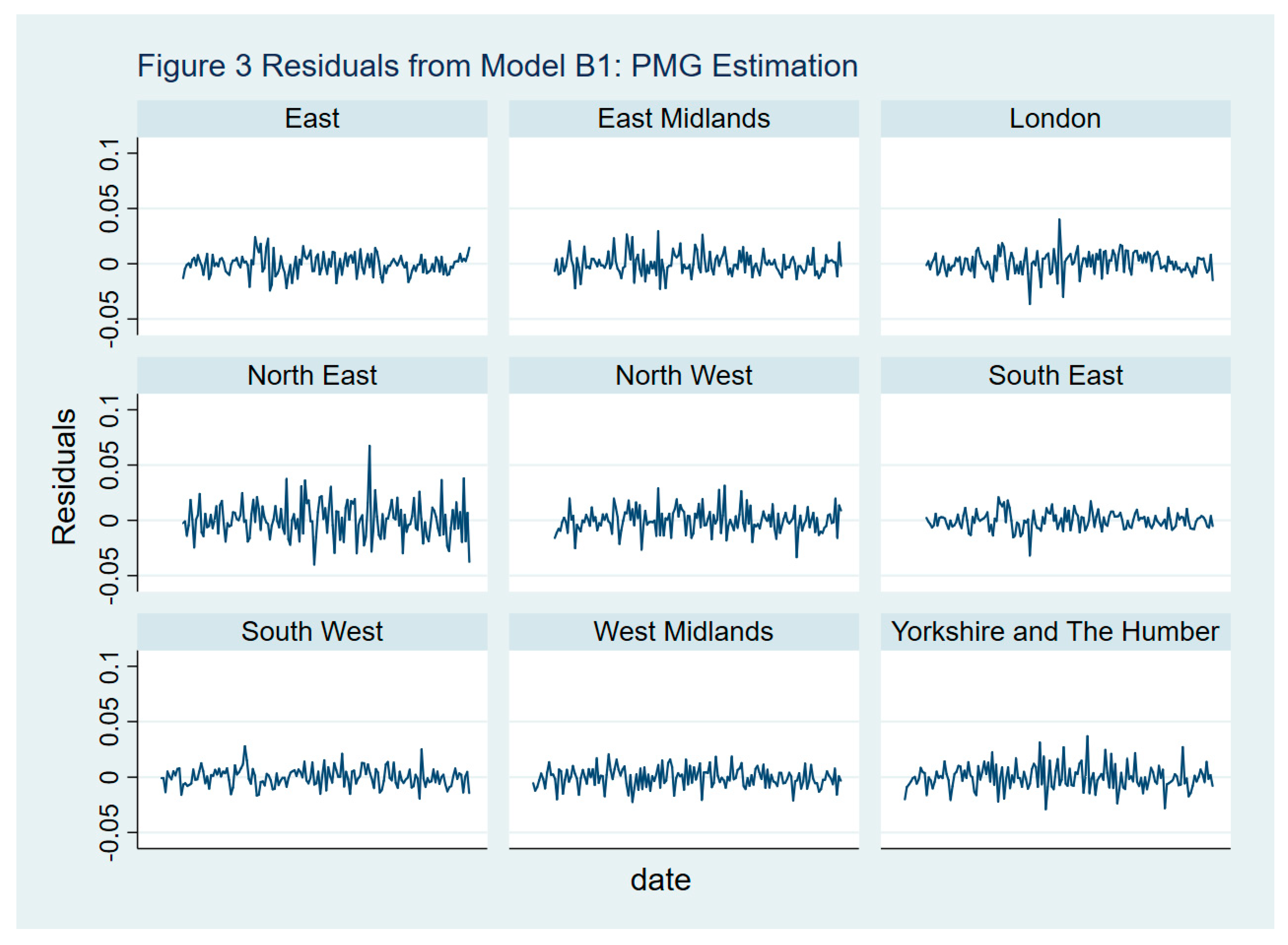
Figure 3 shows the residuals of the PMG results of Model B1. The residuals series fluctuate a lot, which indicates autocorrelation. The moving average in London shows more clearly a regime shift in the residuals during the financial crisis period. Moreover, both London and North East generate more volatile residuals, especially, both fluctuate to a greater extent during the financial crisis.

4.4. Financial Crisis Test

In order to test the potential regime shift during the financial crisis, we include a dummy variable “CRISIS” in our Model B1. We define the period for the financial crisis from August 2007 to August 2011. Figure 4 shows the growing trend of UK monthly housing price index, which is represented by the dotted line together with the actual HPI. Our dummy variable “CRISIS” equals one for the time period from August 2007 to August 2011, and zero outside this period.

Table 5. Pooled Mean Group Results with CRISIS dummy based on Model B1.

Variable	Dependent Variable: Rent to Price Ratio
	Coefficients	Standard Errors
Long-Run Equation
Residential Mortgage Rate	5.708 ***	0.777
Earnings Ratio	−26.526 ***	1.669
10-Year Government real bond rate	−2.190 ***	0.616
CRISIS	0.004 ***	0.001
Short-Run Equation
EC	−0.058 ***	0.010
CRISIS	−0.036 ***	0.006
Δ Rent to Price Ratiot−1	−0.101 ***	0.027
Δ Rent to Price Ratiot−2	0.164 ***	0.027
Δ Residential Mortgage Ratet	−1.245 ***	0.204
Δ Residential Mortgage Ratet−1	0.221 ***	0.563
Δ Residential Mortgage Ratet−2	−0.045 ***	0.530
Δ Residential Mortgage Ratet−3	0.099 ***	0.169
Δ Earnings ratiot	−5.247 ***	1.275
Δ Earnings ratiot−1	6.842 ***	1.756
Δ Earnings ratiot−2	−3.476 ***	0.881
Δ 10-Year Government real bond ratet	−0.452 ***	0.109
Δ 10-Year Government real bond ratet−1	1.243 ***	0.177
Δ 10-Year Government real bond ratet−2	−0.871 ***	0.135
Δ 10-Year Government real bond ratet−3	0.207 ***	0.045
Constant	0.106 ***	0.018
Observations	1404

Note: ***, **, and * represent statistical significance at the 1 percent, 5 percent, and 10 percent level, respectively.

presents the results from the PMG estimations incorporating our dummy variable for the financial crisis period in the estimated equation.

The coefficients of “CRISIS” are significant in both the long-term and short-run equation. They are significantly positive, which means that the crisis was an important factor affecting house price growth in the long term. The signs and coefficients of both the long-run and short-run fundamental variables are the same as those in Model B1 in Table 3.

To get a more detailed picture of the period, we simulated the fundamentals to see how much of the actual change in the rent to price ratio by region was explained by the predictions of the estimated fundamentals models during the pre-crisis period (January 2005 to July 2007), crisis period (August 2007 to August 2011), and post-crisis period (September 2011 to December 2017). We can conclude from

Table 6. Pooled mean group results during different time period based on Model B1.

Variable	Dependent Variable: Rent to Price Ratio
	Pre-Financial Crisis	Financial Crisis	Post-Financial Crisis
Long-Run Equation
Residential Mortgage Rate	3.6212 (5.012)	2.481 *** (7.190)	−10.330 *** (3.450)
Earnings Ratio	−16.493 ** (2.241)	−19.076 *** (−16.963)	−26.824 *** (4.940)
10-Year Government real bond rate	−1.5992 (2.620)	−1.785 *** (−7.160)	0.744 ** (0.288)
Short-Run Equation
EC	0.013 (0.083)	−0.276 *** (−11.353)	−0.184 *** (0.033)
Δ Rent to Price Ratiot−1	0.034 (0.543)	−0.048 (0.048)	−0.214 *** (−5.510)
Δ Rent to Price Ratiot−2	0.037 (0.597)	0.241 *** (0.048)	0.012 (0.331)
Δ Residential Mortgage Ratet	−0.323 (−0.555)	−2.620 *** (−6.679)	0.961 (1.750)
Δ Residential Mortgage Ratet−1	0.986 (1.694)	2.848 *** (3.541)	0.446 (0.730)
Δ Residential Mortgage Ratet−2	1.490 * (2.222)	−2.137 ** (-2.621)	1.755 ** (2.790)
Δ Residential Mortgage Ratet−3	−2.374 *** (−3.553)	0.752 ** (2.667)	−0.233 (−0.395)
Δ Earnings ratiot	−5.112 ** (−2.837)	5.323 (1.930)	−3.232 * (−2.421)
Δ Earnings ratiot−1	5.041 * (2.386)	−5.291 (−1.821)	−0.355 (−0.209)
Δ Earnings ratiot−2	−6.712 *** (−3.648)	2.585 * (1.967)	−4.319 ** (−3.223)
Δ 10-Year Government real bond ratet	0.563 * (2.292)	0.880 ** (3.265)	0.204 (1.752)
Δ 10-Year Government real bond ratet−1	−0.863 *** (−3.451)	−0.593 (−1.385)	−0.002 (−0.015)
Δ 10-Year Government real bond ratet−2	0.285 (1.225)	0.284 (0.876)	−0.447 *** (−3.926)
Δ 10-Year Government real bond ratet−3	−1.121 *** (−4.408)	−0.063 (−0.756)	−0.375 *** (−3.352)
Constant	−0.003 *** (−5.039)	0.480 *** (11.263)	−0.002 *** (−4.238)
Observations	243	441	684

Note: ***, **, and * represent statistical significance at the 1 percent, 5 percent, and 10 percent level, respectively. t-statistics are in parentheses.

that the residential mortgage rate is the most important factor during the financial crisis and after the financial crisis in the long-run. In the short-run, the residential mortgage rate was the most significant factor during the financial crisis, but the sign of lagged terms changed after financial crisis. It is noticeable that the 10-year government real bond rate significantly relates to rent to price ratio in the short-run, except the period during the financial crisis.

5. Discussion

Our results do not confirm a house price bubble at the national level in the United Kingdom; however, the results show that residential property price growth has different short-run momentum at the regional versus the national level. While London shows the strongest short-term momentum and slow return to long-run fundamentals, it cannot strictly be classified as a price bubble, but it clearly shows a short-run shift during the financial crisis. The stronger momentum in London could also be caused by regulation, restrictive planning law, and limited provision of building areas resulting in a temporal mismatch of demand and supply. Housing supply in London tends to be behind demand, as a result of high demand from international investors looking for a safe haven to invest their money. The lag of this additional demand factors in other U.K. regions results in more moderate house price growth. However, low mortgage rates and high first time buyer earnings ratios have also stimulated house price growth across regions at a different pace.

Overall, price growth is strongly influenced by the first time buyer earnings ratio and the variable residential mortgage rate, while the 10-year government bond rate shows less relevance in certain periods. On a regional level prices show varying speeds of reversion to long-run fundamentals, but each region displays different long-run and short-run patterns. The regional house price series has been adjusted for inflation using the national CPI index. However, if we take the perspective of a homeowner in a regional housing market, regional inflation rates would be the right choice because some of the regional markets are largely influenced by local economics, such as the level of economic development or the general economic climate (e.g., London and the North). However, there are no CPI data available on regional level.

The analysis of separating the sample into pre-crisis, crisis, and post crisis period provides further inside into short-run momentum versus long-run fundamentals. Government policies of quantitative easing and lowering of interest rates have changed the relationship between government real bond rates and house price growth. While historically, house prices have been highly correlated with government bond rates, our model could not identify a co-integrating relationship in the long-run. As a result, they also show no significance during the crisis period. Hence, the variable mortgage rate adjusted for inflation seems to be a better predictor for house price growth. We believe that this is a short term effect and as government real bond rates return to positive levels, this will restore the long-run relationship with residential housing markets.

Overall, we can conclude that short-term determinants of houses prices have shifted away from long-term indicators at varying degrees on a regional level, but we cannot confirm that these short-term effects result in sufficient momentum to be considered a house price bubble in the regions.

References

- Abraham, Jesse M., and Patric H. Hendershott. 1993. Patterns and Determinants of Metropolitan House Prices, 1977–91 (October 1992). NBER Working Paper No. w4196. Available online: https://ssrn.com/abstract=879241 (accessed on 12 September 2018).
- Abraham, Jesse M., and Patric H. Hendershott. 1996. Bubbles in metropolitan housing markets. Journal of Housing Research 7: 191–207. [Google Scholar] [CrossRef]
- Barrell, Ray, Simon Kirby, and Rebecca Riley. 2004. The Current Position of UK House Prices. National Institute Economic Review 189: 57–60. [Google Scholar] [CrossRef]
- Black, Angela, Patricia Fraser, and Martin Hoesli. 2006. House Prices, Fundamental and Bubbles. Journal of Business Finance and Accounting 33: 1535–55. [Google Scholar] [CrossRef]
- Chan, Hing Lin, Shu Kam Lee, and Kai Yin Woo. 2001. Detecting Rational Bubbles in the Residential Housing Markets in Hong Kong. Economic Modelling 18: 61–73. [Google Scholar] [CrossRef]
- Cutler, David M., James M. Poterba, and Lawrence H. Summers. 1991. Speculative dynamics. The Review of Economic Studies 58: 529–46. [Google Scholar] [CrossRef]
- Fama, Eugene F., and Kenneth R. French. 1988. Dividend yields and expected stock returns. Journal of financial economics 22: 3–25. [Google Scholar] [CrossRef]
- Favilukis, Jack, Sydney C. Ludvigson, and Stijn Van Nieuwerburgh. 2017. The macroeconomic effects of housing wealth, housing finance, and limited risk-sharing in general equilibrium. Journal of Political Economy 125: 140–223. [Google Scholar] [CrossRef]
- Flood, Robert P., and Robert J. Hodrick. 1990. On testing for speculative bubbles. Journal of Economic Perspectives 4: 85–101. [Google Scholar] [CrossRef]
- Gholipour, Hassan Fereidouni, Usama Al-mulali, and Abdul Hakim Mohammed. 2014. Foreign investments in real estate, economic growth and property prices: Evidence from OECD countries. Journal of Economic Policy Reform 17: 33–45. [Google Scholar] [CrossRef]
- Giglio, Stefano, Matteo Maggiori, and Johannes Stroebel. 2016. No-bubble condition: Model-free tests in housing markets. Econometrica 84: 1047–91. [Google Scholar] [CrossRef]
- Glaeser, Edward L., Joseph Gyourko, and Albert Saiz. 2008. Housing supply and housing bubbles. Journal of Urban Economics 64: 198–217. [Google Scholar] [CrossRef] [Green Version]
- Glaeser, Edward L., Joshua D. Gottlieb, and Joseph Gyourko. 2010. Can Cheap Credit Explain the Housing Boom? In NBER book Housing and the Financial Crisis (2013). Edited by Edward L. Glaeser and Todd Sinai. Chicago: University of Chicago Press, pp. 301–59. [Google Scholar]
- Glaeser, Edward L., and Charles G. Nathanson. 2017. An extrapolative model of house price dynamics. Journal of Financial Economics 126: 147–70. [Google Scholar] [CrossRef]
- Goodman, Allen C., and Thomas G. Thibodeau. 2008. Where are the speculative bubbles in US housing markets? Journal of Housing Research 17: 117–37. [Google Scholar] [CrossRef]
- Hadri, Kaddour. 2000. Testing for stationarity in heterogeneous panel data. The Econometrics Journal 3: 148–61. [Google Scholar] [CrossRef]
- Himmelberg, Charles, Christopher Mayer, and Todd Sinai. 2005. Assessing high house prices: Bubbles, fundamentals, and misperceptions. Journal of Economic Perspectives 19: 67–92. [Google Scholar] [CrossRef]
- Im, Kyung So, M. Hashem Pesaran, and Yongcheol Shin. 2003. Testing for unit roots in heterogeneous panels. Journal of Econometrics 115: 53–74. [Google Scholar] [CrossRef]
- Khandani, Amir E., Andrew W. Lo, and Robert C. Merton. 2013. Systemic risk and the refinancing ratchet effect. Journal of Financial Economics 108: 29–45. [Google Scholar] [CrossRef] [Green Version]
- Lai, Rose N., and Robert A. Van Order. 2010. Momentum and house price growth in the United States: Anatomy of a bubble. Real Estate Economics 38: 753–73. [Google Scholar] [CrossRef]
- Lai, Rose Neng, and Robert Van Order. 2017. US House Prices over the Last 30 Years: Bubbles, Regime Shifts and Market (In) Efficiency. Real Estate Economics 45: 259–300. [Google Scholar] [CrossRef]
- Mayer, Christopher, and Todd Sinai. 2009. U.S. House Price Dynamics and Behavioral Finance. In Policy Making Insights from Behavioral Economics. Edited by Christopher L. Foote, Lorenz Goette and Stephan Meier. Boston: Federal Reserve Bank of Boston, chp. 5. [Google Scholar]
- Meese, Richard, and Nancy Wallace. 1994. Testing the present value relation for housing prices: Should I leave my house in San Francisco? Journal of Urban Economics 35: 245–66. [Google Scholar] [CrossRef]
- Mikhed, Vyacheslav, and Petr Zemčík. 2009. Testing for bubbles in housing markets: A panel data approach. The Journal of Real Estate Finance and Economics 38: 366–86. [Google Scholar] [CrossRef]
- Nickell, Steve. 2005. Practical Issues in UK Monetary Policy, 2000–2005. Keynes Lecture in Economics. London: British Academy. [Google Scholar] [CrossRef]
- Paul, Biru Paksha, Md Gazi Salah Uddin, and Abdullah M. Noman. 2011. Remittances and output in Bangladesh: An ARDL bounds testing approach to cointegration. International Review of Economics 58: 229–42. [Google Scholar] [CrossRef]
- Peláez, Rolando F. 2012. The housing bubble in real-time: The end of innocence. Journal of Economics and Finance 36: 211–25. [Google Scholar] [CrossRef]
- Pesaran, M. Hashem, and Ron Smith. 1995. Estimating long-run relationships from dynamic heterogeneous panels. Journal of Econometrics 68: 79–113. [Google Scholar] [CrossRef]
- Hasham, Pesaran M., Shin Yongcheol, and P. Smith Ron. 1997. Pooled Estimation of Long-Run Relationships in Dynamic Heterogeneous Panels. Cambridge Working Paper in Economics, Cambridge. August. Available online: https://EconPapers.repec.org/RePEc:cam:camdae:9721 (accessed on 12 September 2018).
- Pesaran, M. Hashem. 2007. Simple panel unit root test in the presence of cross-section dependence. Journal of Applied Econometrics 22: 265–312. [Google Scholar] [CrossRef]
- Hwang, Min, and John M. Quigley. 2006. Economic fundamentals in local housing markets: evidence from US metropolitan regions. Journal of Regional Science 46: 425–53. [Google Scholar] [CrossRef]
- Rodríguez, Carlos, and Ricardo Bustillo. 2010. Modelling Foreign Real Estate Investment: The Spanish Case. The Journal of Real Estate Finance and Economics 41: 354. [Google Scholar] [CrossRef]
- Rogers, Dallas, Chyi Lin Lee, and Ding Yan. 2015. The Politics of Foreign Investment in Australian Housing: Chinese Investors, Translocal Sales Agents and Local Resistance. Housing Studies 30: 730–48. [Google Scholar] [CrossRef]
- Stiglitz, Joseph E. 1990. Symposium on bubbles. Journal of Economic Perspectives 4: 13–18. [Google Scholar] [CrossRef]
- West, Kenneth D. 1987. A specification test for speculative bubbles. The Quarterly Journal of Economics 102: 553–80. [Google Scholar] [CrossRef]
- Taipalus, Katja. 2006. A Global House Price Bubble? Evaluation Based on a New Rent-Price Approach. Bank of Finland Research Discussion Paper No. 29/2006. Available online: https://ssrn.com/abstract=1018329 (accessed on 12 September 2018). [CrossRef]
- Westerlund, Joakim. 2007. Testing for error correction in panel data. Oxford Bulletin of Economics and Statistics 69: 709–48. [Google Scholar] [CrossRef]