Refined Measures of Dynamic Connectedness based on Time-Varying Parameter Vector Autoregressions

Abstract

In this study, we enhance the dynamic connectedness measures originally introduced by Diebold and Yılmaz (2012, 2014) with a time-varying parameter vector autoregressive model (TVP-VAR) which predicates upon a time-varying variance-covariance structure. This framework allows to capture possible changes in the underlying structure of the data in a more flexible and robust manner. Specifically, there is neither a need to arbitrarily set the rolling-window size nor a loss of observations in the calculation of the dynamic measures of connectedness, as no rolling-window analysis is involved. Given that the proposed framework rests on multivariate Kalman filters, it is less sensitive to outliers. Furthermore, we emphasise the merits of this approach by conducting Monte Carlo simulations. We put our framework into practice by investigating dynamic connectedness measures of the four most traded foreign exchange rates, comparing the TVP-VAR results to those obtained from three different rolling-window settings. Finally, we propose uncertainty measures for both TVP-VAR-based and rolling-window VAR-based dynamic connectedness measures.

1. Introduction

Investigating the propagation of financial crises into the economy has been at the epicenter of academic research in recent years, especially in the aftermath of the global financial crisis of 2007–2009. On general principles, crises are unpredictable; however, transmission mechanisms relating to financial turmoil do share certain similarities (Reinhart and Rogoff 2008). In turn, researchers have developed elaborate methods aiming to capture transmission mechanisms that relate to such events.

A notable empirical method is the one by Diebold and Yılmaz (2009, 2012, 2014) who introduced a variety of connectedness measures based on the notion of the forecast error variance decomposition that was derived from the rolling-window VARs. In the present study, we provide an extension to the Diebold and Yılmaz (2014) connectedness approach by applying a time-varying parameter vector autoregressive model (TVP-VAR) with a time-varying covariance structure, as opposed to the constant-parameter rolling-window VAR approach.1

The Diebold and Yılmaz (2009, 2012, 2014) VAR-based connectedness approach has already attracted significant attention by the existing economic and financial literature, and has been applied to issues relating to the stock market interdependencies, volatility spillovers, business cycle spillovers, as well as bond yield spillovers (see, inter alia, Alter and Beyer 2014; Antonakakis 2012; Awartani and Maghyereh 2013; Bekaert et al. 2014; Bubák et al. 2011; Diebold and Yilmaz 2015; McMillan and Speight 2010). At the same time, alternative measures of connectedness have been provided by Baruník et al. (2016, 2017), Baruník and Křehlík (2018), and Geraci and Gnabo (2018).

It would be instructive at this point to note that the Diebold and Yılmaz (2009, 2012, 2014) approach facilitates the measurement of interdependence across a network of variables, thus providing a framework for analysing both an idiosyncratic influence (i.e., own) and influence by others (i.e., network). the ensuing measures predicate upon the estimation of the forecast error variance decompositions that derive from a VAR model. In addition, these measures allow to further classify interdependence and provide granulated information, considering the fact that results can be obtained for (i) aggregate, (ii) directional, as well as (iii) net interdependence. More particularly, as far as net interdependence is concerned, this measure allows for distinguishing between net shock transmitters and net shock receivers, which in turn helps attain a better understanding of the underlying dynamics and facilitates the formulation of policy implications. As a final step, the dynamic nature of interconnectedness is typically being investigated through the use of the rolling-windows approach, whereby the researcher begins by deciding upon the relevant window length and forecast horizon. What is more, it should be noted that in their 2009 study, Diebold and Yilmaz investigated the interdependence across the variables of interest by utilising a Cholesky-type VAR framework (i.e., where the ordering of the variables affects outcomes), whereas in their 2012 study, they utilised a generalised VAR approach (i.e., where the ordering of the variables is irrelevant). Finally, in their 2014 study, Diebold and Yilmaz emphasized the concept of connectedness and offered ways to measure connectedness based on their previous relevant research.

This extension improves the existing method in four ways: (i) potential changes in the values of the parameters can be more accurately determined, (ii) outliers do not affect outcomes, (iii) there is no need to set an arbitrary rolling-window size, and (iv) there is no loss of observations in the calculation of the dynamic measures. To be more explicit, while the last two improvements are rather created by construction, the first two can be evidenced by the application of Monte Carlo simulations. In point of fact, when we test the robustness of our estimations, both in terms of outliers’ sensitivity and changes in the values of the parameters, the results indicate that the TVP-VAR estimations are superior to those generated by rolling-windows.

In turn, we illustrate the accuracy of our proposed method by considering connectedness in the foreign exchange market. More specifically, we collect monthly data on the exchange rate between the USD and the following currencies: (i) EUR/EC, (ii) GBP, (iii) CHF, and (iv), JPY. the choice of the currencies was based on their respective position on the list of the most traded currencies of the world. the USD ranks first, and in this regard, it serves as the base currency of the study. Subsequently, we estimate results for different window-lengths (i.e., 25, 26, …, 274, 275 months) in order to (i) deduct how dynamic total connectedness changes with the window size, and (ii) contrast these results with those obtained from our TVP-VAR approach. We find that our proposed TVP-VAR-based measure of connectedness is similar to the averaged dynamic connectedness measures of the rolling-window VAR model; nonetheless, TVP-VAR values immediately adjust to underlying events, while rolling-window-based estimates either overreact (given an inadequate window size) or smooth out the effect (given a large window size).

In line with the aforementioned analysis, we then select three window sizes that are neither too large nor too small. In particular, we choose 50, 100, and 200 observations-wide windows. Windows were chosen on the basis of their mean absolute prediction error (MAPE) value stemming from a 12-step-ahead forecast. Prominent among our results is the fact that (i) the TVP-VAR model exhibits similar trend-movements to the 50-month rolling-windows VAR; nonetheless, the latter is much less volatile, and (ii) despite how the 100-month rolling-windows VAR is as persistent as its TVP counterpart, it does not appear to adjust to changes as quickly as the TVP-VAR model.

Finally, we utilise the results from our empirical application in order to provide two additional inputs to the existing literature. First, we propose a method to generate confidence intervals of dynamic connectedness by combining bootstrapped generalised impulse response functions (see, Koop et al. 1996; Pesaran and Shin 1998) with the joint confidence bands for impulse response functions suggested by Lütkepohl et al. (2015). This combined approach refines the intervals approach introduced by Kilian (1998, 1999). Second, we offer an uncertainty estimation of TVP-VAR-based connectedness measures by letting forgetting factors and Minnesota priors vary randomly.

It would also be instructive at this point to note that, so far, there have been two seminal studies in the field of dynamic connectedness through TVP-VARs; namely, Antonakakis and Gabauer (2017) and Korobilis and Yilmaz (2018). Both studies adopt a similar framework, although they investigate different issues. To be more explicit, Antonakakis and Gabauer (2017) provided evidence of the superiority of TVP-VAR connectedness estimations using the exchange rate market as a point of reference, whereas Korobilis and Yilmaz (2018) provided similar evidence by using the stock market as a point of reference. The present study constitutes a more detailed and complete illustration of the analysis provided by Antonakakis and Gabauer (2017), as three rolling-window sizes have been chosen based upon the mean absolute prediction error, which is better than just an arbitrarily chosen window size, as in the original paper. Furthermore, we have provided a prior sensitivity analysis, uncertainty intervals for all connectedness measures, and finally, have evaluated the forecasting performance of the suggested approach. All of the above further strengthen the argument in favor of TVP-VAR-generated connectedness measures. It should also be noted that, despite the rather scarce literature on TVP-VAR dynamic connectedness, studies in this area have gradually started to emerge (see, inter alia, Gabauer and Gupta 2018; Antonakakis et al. 2018, 2019, 2019a, 2019b; Chatziantoniou and Gabauer 2019), signifying a rather promising area for future research.

In retrospect, this study contributes to the existing literature in a number of ways. First, it provides the framework for generating refined measures of connectedness based on a time-varying VAR modeling approach. Second, it allows for presenting new evidence regarding the exchange-rate connectedness of some of the most popular currencies of the world. Finally, it facilitates both the introduction of alternative specifications of error bounds and the implementation of a thorough sensitivity analysis.

The remainder of this study is organized as follows. In Section 2 we describe our proposed method, whereas in Section 3 we illustrate its advantages by applying Monte Carlo simulations. In Section 4 we provide a description of the employed dataset. In Section 5 we proceed with the empirical comparison between the various connectedness measures. Finally, Section 6 concludes the study.

2. Methodology

TVP-VAR

Our proposed TVP-VAR method extends the originally proposed connectedness approach of Diebold and Yılmaz (2014) by allowing the variance-covariance matrix to vary via a Kalman filter estimation with forgetting factors in the spirit of Koop and Korobilis (2014). By doing so, our method (i) overcomes the burden of the often arbitrarily chosen rolling-window size, that could lead to very erratic or flattened parameters, and (ii) avoids the loss of valuable observations. In this respect, this method may also be employed to examine dynamic connectedness measures for both low-frequency data and limited time-series data. Furthermore, Koop and Korobilis (2014) point out that the heteroscedastic procedure outperforms its homoscedastic counterpart.

The TVP-VAR(p) model can be written as follows:

$$\begin{array}{ccc}\hfill {\mathit{y}}_t=& {\mathit{A}}_t{\mathit{z}}_{t-1}+{\mathit{ϵ}}_t\hfill & \hfill {\mathit{ϵ}}_t|{\mathsf{\Omega }}_{t-1}\sim N(\mathbf{0},{\mathsf{\Sigma }}_t)\end{array}$$

(1)

$$\begin{array}{ccc}\hfill vec\left({\mathit{A}}_t\right)=& vec\left({\mathit{A}}_{t-1}\right)+{\mathit{\xi }}_t\hfill & \hfill {\mathit{\xi }}_t|{\mathsf{\Omega }}_{t-1}\sim N(\mathbf{0},{\mathsf{\Xi }}_t)\end{array}$$

(2)

with

$$\begin{array}{c}\hfill {\mathit{z}}_{t-1}=\left(\begin{array}{c}{\mathit{y}}_{t-1}\\ {\mathit{y}}_{t-2}\\ ⋮\\ {\mathit{y}}_{t-p}\end{array}\right){\mathit{A}}_t^{\prime }=\left(\begin{array}{c}{\mathit{A}}_{1t}\\ {\mathit{A}}_{2t}\\ \dots \\ {\mathit{A}}_{pt}\end{array}\right)\end{array}$$

where ${\mathsf{\Omega }}_{t-1}$ represents all information available until t−1, ${\mathit{y}}_t$ and ${\mathit{z}}_{t-1}$ represents $m\times 1$ and $mp\times 1$ vectors, respectively, ${\mathit{A}}_t$ and ${\mathit{A}}_{it}$ are $m\times mp$ and $m\times m$ dimensional matrices, respectively, ${\mathit{ϵ}}_t$ is an $m\times 1$ vector, and ${\mathit{\xi }}_t$ is an $m^{2}p\times 1$ dimensional vector, whereas the time-varying variance-covariance matrices ${\mathsf{\Sigma }}_t$ and ${\mathsf{\Xi }}_t$ are $m\times m$ and $m^{2}p\times m^{2}p$ dimensional matrices, respectively. Moreover, $vec\left({\mathit{A}}_t\right)$ is the vectorisation of ${\mathit{A}}_t$ which is an $m^{2}p\times 1$ dimensional vector.

For the initialization of the Kalman filter, we used the Primiceri (2005) and Del Negro and Primiceri (2015) prior. Hence, in our study, we set ${\mathit{A}}_{OLS}$, ${\mathsf{\Sigma }}_{OLS}^A$, and ${\mathsf{\Sigma }}_{OLS}$ as equal to the VAR estimation results of the first 60 months:

$$\begin{array}{cc}\hfill vec\left({\mathit{A}}_0\right)\sim & N(vec\left({\mathit{A}}_{OLS}\right),{\mathsf{\Sigma }}_{OLS}^A)\hfill \\ \hfill {\mathsf{\Sigma }}_0=& {\mathsf{\Sigma }}_{OLS}.\hfill \end{array}$$

In the interests of numerical stability, we implement decay factors in the Kalman filter algorithm. the choice of decay factors resembles the choice of priors in general, and depends on the expected amount of time variation in the parameters. In this study, we consider the benchmark values for ${\kappa }_1$ and ${\kappa }_2$ provided by the Koop and Korobilis (2014) study, according to which ${\kappa }_1=0.99$ and ${\kappa }_2=0.96$. It should also be stressed that even though estimation procedures are available which allow the decay factors to vary over time, we keep them constant at fixed values, since Koop and Korobilis (2013) found that the value added by time-varying decay factors with respect to the forecasting performance was questionable and increased the computation burden of the Kalman filter algorithm significantly. In turn, the multivariate Kalman filter can be formulated as follows:

$$\begin{array}{cc}\hfill vec\left({\mathit{A}}_t\right)|{\mathit{z}}_{1:t-1}\sim & N(vec\left({\mathit{A}}_{t|t-1}\right),{\mathsf{\Sigma }}_{t|t-1}^A)\hfill \\ \hfill {\mathit{A}}_{t|t-1}=& {\mathit{A}}_{t-1|t-1}\hfill \\ \hfill {\mathit{ϵ}}_t=& {\mathit{y}}_t-{\mathit{A}}_{t|t-1}{\mathit{z}}_{t-1}\hfill \\ \hfill {\mathsf{\Sigma }}_t=& {\kappa }_2{\mathsf{\Sigma }}_{t-1|t-1}+(1-{\kappa }_2){\mathit{ϵ}}_t^{\prime }{\mathit{ϵ}}_t\hfill \\ \hfill {\mathsf{\Xi }}_t=& (1-{\kappa }_1^{-1}){\mathsf{\Sigma }}_{t-1|t-1}^A\hfill \\ \hfill {\mathsf{\Sigma }}_{t|t-1}^A=& {\mathsf{\Sigma }}_{t-1|t-1}^A+{\mathsf{\Xi }}_t\hfill \\ \hfill {\mathsf{\Sigma }}_{t|t-1}=& {{\mathit{z}}_{t-1}{\mathsf{\Sigma }}_{t|t-1}^A{\mathit{z}}_{t-1}^{\prime }+\mathsf{\Sigma }}_t\hfill \end{array}$$

We updated ${\mathit{A}}_t$, ${\mathsf{\Sigma }}_t^A$, and ${\mathsf{\Sigma }}_t$, given the information at time t, by the following steps:

$$\begin{array}{cc}\hfill vec\left({\mathit{A}}_t\right)|{\mathit{z}}_{1:t}\sim & N(vec\left({\mathit{A}}_{t|t}\right),{\mathsf{\Sigma }}_{t|t}^A)\hfill \\ \hfill {\mathit{K}}_t=& {\mathsf{\Sigma }}_{t|t-1}^A{\mathit{z}}_{t-1}^{\prime }{\mathsf{\Sigma }}_{t|t-1}^{-1}\hfill \\ \hfill {\mathit{A}}_{t|t}=& {\mathit{A}}_{t|t-1}+{\mathit{K}}_t({\mathit{y}}_t-{\mathit{A}}_{t|t-1}{\mathit{z}}_{t-1})\hfill \\ \hfill {\mathsf{\Sigma }}_{t|t}^A=& (\mathit{I}-{\mathit{K}}_t){\mathsf{\Sigma }}_{t|t-1}^A\hfill \\ \hfill {\mathit{ϵ}}_{t|t}=& {\mathit{y}}_t-{\mathit{A}}_{t|t}{\mathit{z}}_{t-1}\hfill \\ \hfill {\mathsf{\Sigma }}_{t|t}=& {\kappa }_2{\mathsf{\Sigma }}_{t-1|t-1}+(1-{\kappa }_2){\mathit{ϵ}}_{t|t}^{\prime }{\mathit{ϵ}}_{t|t},\hfill \end{array}$$

where ${\mathit{K}}_t$ represents the Kalman gain that explains by how much the parameters, ${\mathit{A}}_t$, should be changed in any given state. On the one hand, if the parameter uncertainty, ${\mathsf{\Sigma }}_{t|t-1}^A$ is small (large), it means that the parameters, ${\mathit{A}}_t$, should be similar to (adjusted to) their prior states. On the other hand, if the error variance ${\mathsf{\Sigma }}_t$ is small (large), meaning that the estimation is very accurate (inaccurate), the parameters, ${\mathsf{\Phi }}_t$, should be similar to (adjusted to) their prior values.

The time-varying coefficients and time-varying variance-covariance matrices are used to estimate the generalized connectedness procedure of Diebold and Yılmaz (2014) that is based on generalized impulse response functions (GIRF) and generalized forecast error variance decompositions (GFEVD) in accordance with Koop et al. (1996) and Pesaran and Shin (1998). In order to calculate the GIRF and GFEVD, we transform the TVP-VAR to its vector moving average (VMA) representation based on the Wold representation theorem. Retrieving the VMA representation can be illustrated by recursive substitution:

$$\begin{array}{}\mathrm{(3)}& \hfill {\mathit{y}}_t& =& {\mathit{J}}^{\prime }({\mathit{M}}_t({\mathit{z}}_{t-2}+{\mathit{\eta }}_{t-1})+{\mathit{\eta }}_t)\hfill \mathrm{(4)}& & \hfill =& {\mathit{J}}^{\prime }({\mathit{M}}_t({\mathit{M}}_t({\mathit{z}}_{t-3}+{\mathit{\eta }}_{t-2})+{\mathit{\eta }}_{t-1})+{\mathit{\eta }}_t)\hfill \mathrm{(5)}& & \hfill ⋮& \mathrm{(6)}& & \hfill =& {\mathit{J}}^{\prime }({\mathit{M}}_t^{k-1}{\mathit{z}}_{t-k-1}+\sum _{j=0}^k{\mathit{M}}_t^j{\mathit{\eta }}_{t-j})\hfill \end{array}$$

with

$$\begin{array}{c}\hfill {\mathit{M}}_t=\left(\begin{array}{c}{\mathit{A}}_t\\ {\mathit{I}}_{m(p-1)}& {\mathbf{0}}_{m(p-1)\times m}\end{array}\right){\mathit{\eta }}_t=\left(\begin{array}{c}{\mathit{ϵ}}_t\\ \mathbf{0}\\ ⋮\\ \mathbf{0}\end{array}\right)=\mathit{J}{\mathit{ϵ}}_{\mathit{t}}\mathit{J}=\left(\begin{array}{c}\mathit{I}\\ \mathbf{0}\\ ⋮\\ \mathbf{0}\end{array}\right)\end{array}$$

(7)

where ${\mathit{M}}_t$ is an $mp\times mp$ dimensional matrix, ${\mathit{\eta }}_t$ is an $mp\times 1$ dimensional vector, and $\mathit{J}$ is an $mp\times m$ dimensional matrix.

Taking the limit as k approaches ∞ yields to

$$\begin{array}{cc}\hfill {\mathit{y}}_t=& li{m}_{k\to \infty }{\mathit{J}}^{\prime }({\mathit{M}}_t^{k-1}{\mathit{z}}_{t-k-1}+\sum _{j=0}^k{\mathit{M}}_t^j{\mathit{\eta }}_{t-j})=\sum _{j=0}^{\infty }{\mathit{J}}^{\prime }{\mathit{M}}_t^j{\mathit{\eta }}_{t-j},\hfill \end{array}$$

(8)

where it directly follows

$$\begin{array}{}\mathrm{(9)}& \hfill {\mathit{y}}_t=& \sum _{j=0}^{\infty }{\mathit{J}}^{\prime }{\mathit{M}}_t^j\mathit{J}{\mathit{ϵ}}_{t-j}{\mathit{B}}_{jt}={\mathit{J}}^{\prime }{\mathit{M}}_t^j\mathit{J},j=0,1,\dots \hfill \mathrm{(10)}& \hfill {\mathit{y}}_t=& \sum _{j=0}^{\infty }{\mathit{B}}_{jt}{\mathit{ϵ}}_{t-j}\hfill & \end{array}$$

where ${\mathit{B}}_{jt}$ is an $m\times m$ dimensional matrix.

The GIRFs (${\mathsf{\Psi }}_{ij,t}\left(H\right)$) represent the responses of all variables j, following a shock in variable i. Since we did not have a structural model, we computed the differences between an H-step-ahead forecast, once where variable i is shocked and once where variable i is not shocked. the difference can be attributed to the shock in variable i, which can be calculated by

$$\begin{array}{}\mathrm{(11)}& \hfill GIR{F}_t(H,{\mathit{\delta }}_{j,t},{\mathsf{\Omega }}_{t-1})=& E\left({\mathit{y}}_{t+H}\right|{\mathit{e}}_j={\mathit{\delta }}_{j,t},{\mathsf{\Omega }}_{t-1})-E\left({\mathit{y}}_{t+J}\right|{\mathsf{\Omega }}_{t-1})\hfill \mathrm{(12)}& \hfill {\mathsf{\Psi }}_{j,t}\left(H\right)=& \frac{{\mathit{B}}_{H,t}{\mathsf{\Sigma }}_t{\mathit{e}}_j}{\sqrt{{\mathsf{\Sigma }}_{jj,t}}}\frac{{\mathit{\delta }}_{j,t}}{\sqrt{{\mathsf{\Sigma }}_{jj,t}}}{\mathit{\delta }}_{j,t}=\sqrt{{\mathsf{\Sigma }}_{jj,t}}\hfill \mathrm{(13)}& \hfill {\mathsf{\Psi }}_{j,t}\left(H\right)=& {\mathsf{\Sigma }}_{jj,t}^{-\frac{1}{2}}{\mathit{B}}_{H,t}{\mathsf{\Sigma }}_t{\mathit{e}}_j,\hfill \end{array}$$

where ${\mathit{e}}_j$ is an $m\times 1$ selection vector with unity in the jth position, and zero otherwise. In turn, we compute the GFEVD (${\tilde{\varphi }}_{ij,t}\left(H\right)$), which represents the pairwise directional connectedness from j to i and illustrates the influence variable j has on variable i in terms of its forecast error variance share. These variance shares are then normalised, so that each row sums up to one, meaning that all variables together explain 100% of variable i’s forecast error variance. This is calculated as follows:

$$\begin{array}{cc}\hfill {\tilde{\varphi }}_{ij,t}\left(H\right)=& \frac{{\sum }_{t=1}^{H-1}{\mathsf{\Psi }}_{ij,t}^2}{{\sum }_{j=1}^m{\sum }_{t=1}^{H-1}{\mathsf{\Psi }}_{ij,t}^2}\hfill \end{array}$$

(14)

with ${\sum }_{j=1}^m{\tilde{\varphi }}_{ij,t}\left(H\right)=1$ and ${\sum }_{i,j=1}^m{\tilde{\varphi }}_{ij,t}\left(H\right)=m$. the denominator represents the cumulative effect of all the shocks, while the numerator illustrates the cumulative effect of a shock in variable i. Using the GFEVD, we construct the total connectedness index by

$$\begin{array}{cc}\hfill C_t\left(H\right)=& \frac{{\sum }_{i,j=1,i\ne j}^m{\tilde{\varphi }}_{ij,t}\left(H\right)}{{\sum }_{i,j=1}^m{\tilde{\varphi }}_{ij,t}\left(H\right)}\ast 100=\frac{{\sum }_{i,j=1,i\ne j}^m{\tilde{\varphi }}_{ij,t}\left(H\right)}{m}\ast 100.\hfill \end{array}$$

(15)

This connectedness approach shows how a shock in one variable spills over to other variables. First, we look at the case where variable i transmits its shock to all other variables j, called total directional connectedness to others and defined as

$$\begin{array}{cc}\hfill C_{i\to j,t}\left(H\right)=& \frac{{\sum }_{j=1,i\ne j}^m{\tilde{\varphi }}_{ji,t}\left(H\right)}{{\sum }_{j=1}^m{\tilde{\varphi }}_{ji,t}\left(H\right)}\ast 100.\hfill \end{array}$$

(16)

Second, we calculate the directional connectedness variable i receives from variables j, called total directional connectedness from others and defined as

$$\begin{array}{cc}\hfill C_{i\leftarrow j,t}\left(H\right)=& \frac{{\sum }_{j=1,i\ne j}^m{\tilde{\varphi }}_{ij,t}\left(H\right)}{{\sum }_{i=1}^m{\tilde{\varphi }}_{ij,t}\left(H\right)}\ast 100.\hfill \end{array}$$

(17)

Finally, we subtract total directional connectedness to others from total directional connectedness from others to obtain the net total directional connectedness, which can be interpreted as the influence variable i has on the analyzed network.

$$\begin{array}{c}\hfill C_{i,t}=C_{i\to j,t}\left(H\right)-C_{i\leftarrow j,t}\left(H\right)\end{array}$$

(18)

If $C_{i,t}$ is positive, it means that variable i influences the network more than itself being influenced. By contrast, if $C_{i,t}$ is negative, it means that variable i is driven by the network.

Finally, we break down the net total directional connectedness even further to examine the bidirectional relationships by computing the net pairwise directional connectedness,

$$\begin{array}{c}\hfill NPD{C}_{ij}\left(H\right)=\left({\tilde{\varphi }}_{jit}\left(H\right)-{\tilde{\varphi }}_{ijt}\left(H\right)\right)\ast 100.\end{array}$$

(19)

If $NPD{C}_{ij}\left(H\right)>0$$(NPD{C}_{ij}\left(H\right)<0)$, it means that variable i dominates (is dominated by) variable j.

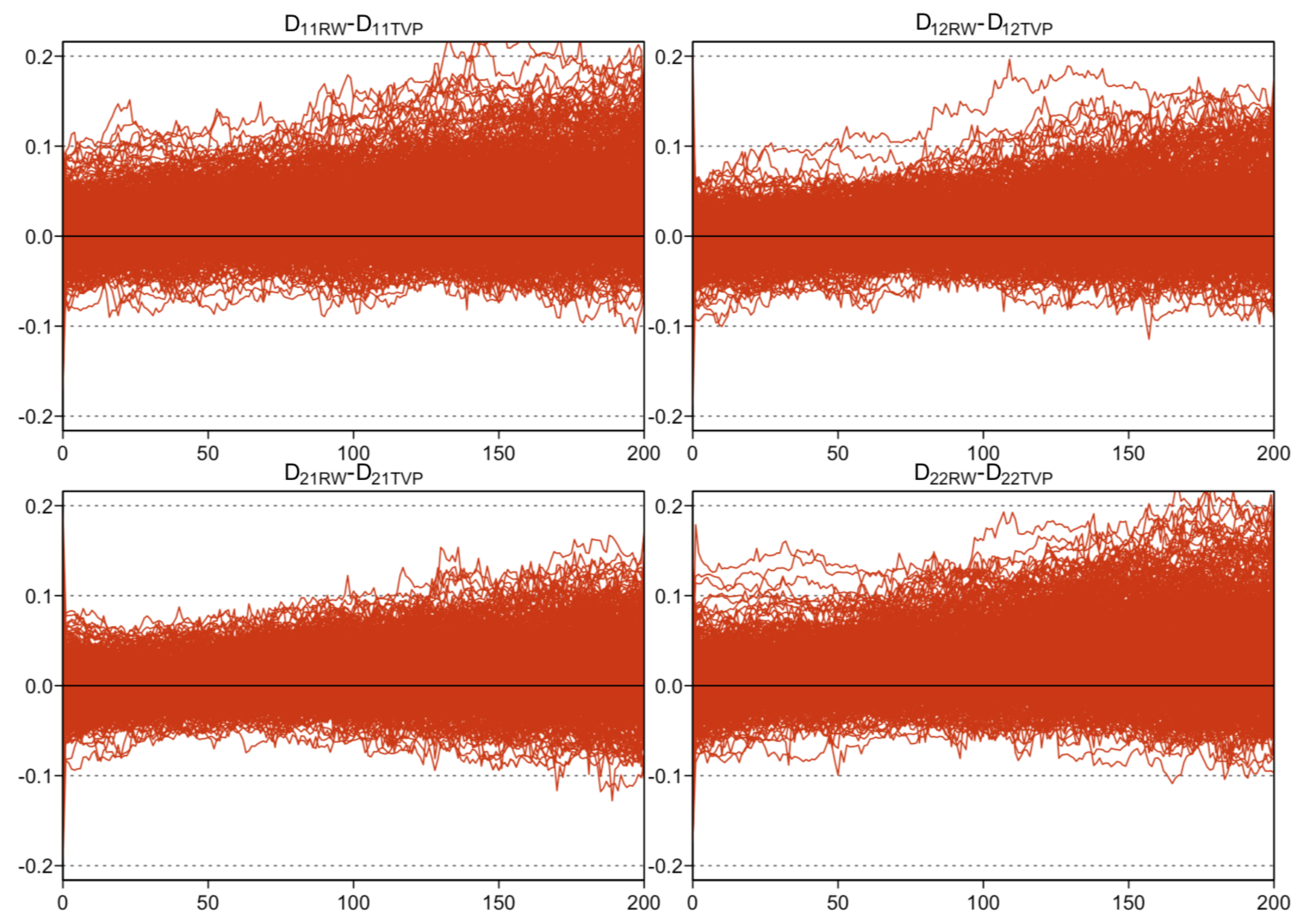
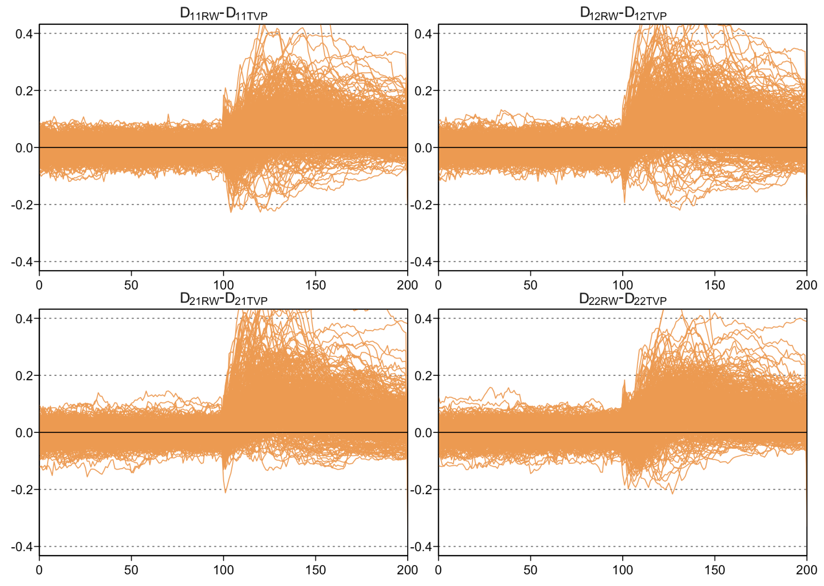
3. Monte Carlo Simulation

In this section, we perform two different kinds of Monte Carlo simulations so as to check whether the TVP-VAR model indeed outperforms the rolling-window VAR in the case of a single outlier and a structural break in the parameters. We simulate the following VAR(1) process:

$${\mathit{y}}_t=\mathit{A}{\mathit{z}}_{t-1}+{\mathit{ϵ}}_t{\mathit{ϵ}}_t|{\mathsf{\Omega }}_{t-1}\sim N(\mathbf{0},\mathit{I}).$$

(20)

Specifically, the simulation for each scenario is repeated 10,000 times, whereas the sample under investigation has a length of 400 and the burn-in phase corresponds to 5000 observations. the Monte Carlo simulation is estimated for various rolling-window sizes (in particular, 50, 100, 150, 200, 250, 300) and VAR models based on up to 10 endogenous variables, which result in qualitatively similar results. For the sake of brevity, we calculate the time-varying parameters with both methods (i.e., 200 observation rolling-window VAR and TVP-VAR2) and compute the absolute deviation between the estimated and the true parameters as follows:

$$\begin{array}{cc}\hfill {\mathit{D}}_{TVP,t}& =|{\mathit{A}}_{TVP,t}-\mathit{A}|\hfill \end{array}$$

(21)

$$\begin{array}{cc}\hfill {\mathit{D}}_{RW,t}& =|{\mathit{A}}_{RW,t}-\mathit{A}|\hfill \end{array}$$

(22)

where ${\mathit{A}}_{TVP,t}$ and ${\mathit{A}}_{RW,t}$ are the estimated time-varying parameters of the TVP-VAR and the rolling-window VAR, respectively, and ${\mathit{D}}_{TVP,t}$ and ${\mathit{D}}_{RW,t}$ are the absolute deviation from the true value ($\mathit{A}$).

Finally, we subtract the aforementioned absolute deviations from each other, as follows:

$$\begin{array}{c}\hfill {\mathit{DV}}_t={\mathit{D}}_{RW,t}-{\mathit{D}}_{TVP,t}.\end{array}$$

(23)

If ${\mathit{DV}}_t>0$ (${\mathit{DV}}_t<0$), then the estimated parameters of the rolling-window VAR model are further away from the true parameters than the TVP-VAR results, which in turn implies that the TVP-VAR is more (less) accurate.

In the first two cases, the coefficient matrix in the Monte Carlo simulation is defined as follows:

$$\begin{array}{c}\hfill {\mathit{A}}_1=\left|\begin{array}{cc}0.6& 0.3\\ 0.3& 0.6\end{array}\right|{\mathit{A}}_2=\left|\begin{array}{cc}0.9& 0.0\\ 0.0& 0.9\end{array}\right|\end{array}$$

(24)

while in the third case, the coefficient matrix is adjusted from ${\mathit{A}}_1$ to ${\mathit{A}}_2$, simulating a structural break in the parameters.

The Monte Carlo simulation results for the aforementioned two cases are shown in Figure 1 and Figure 2 and reported in

Table 1. Monte Carlo simulation results.

	${\mathit{DV}}_{11}$	${\mathit{DV}}_{12}$	${\mathit{DV}}_{21}$	${\mathit{DV}}_{22}$
	(1)	(2)	(3)	(4)
Outlier	0.025 ***	0.016 ***	0.012 ***	0.027 ***
	(0.0003)	(0.0002)	(0.0002)	(0.0003)
Structural Break	0.033 ***	0.040 ***	0.032 ***	0.028 ***
in Parameters	(0.0005)	(0.001)	(0.0005)	(0.0004)

Note: * p < 0.1; ${}^{**}$p< 0.05; *** p< 0.01.

. In every case, we observe that the deviations across the rolling-window VAR and the TVP-VAR results, ${\mathit{DV}}_t$, are significantly positive, indicating that the TVP-VAR model outperforms the rolling-window VAR specification.

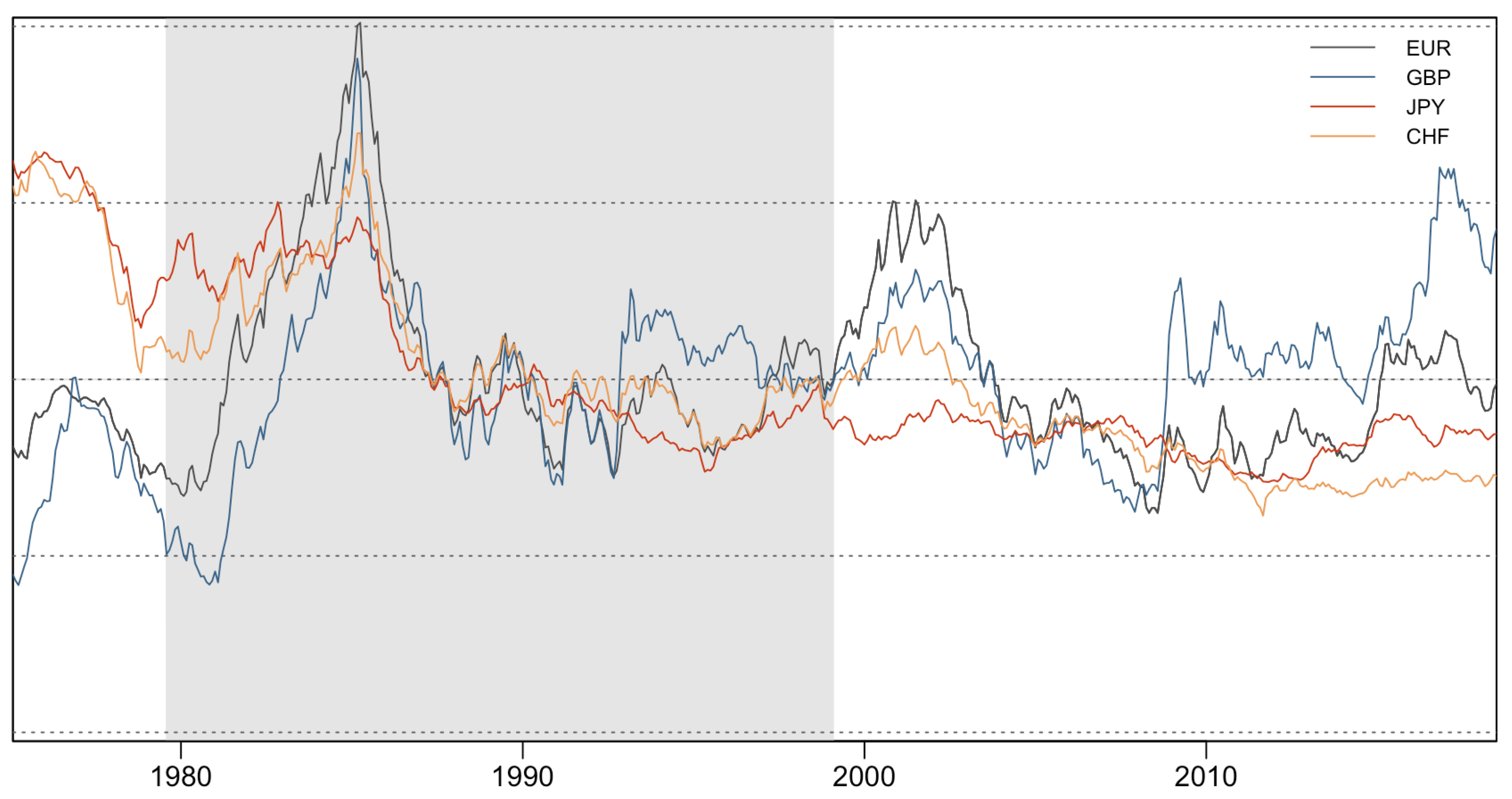
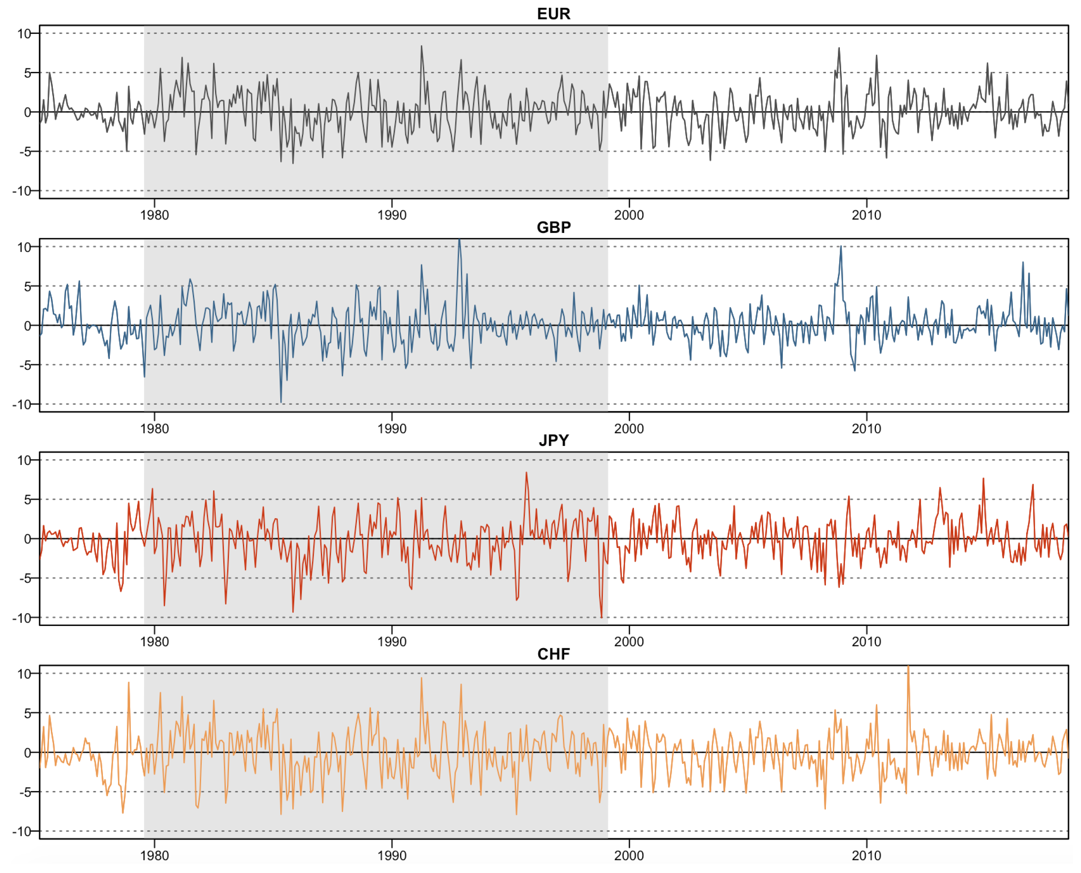
4. Data and Summary Statistics

We employed a dataset that is based on monthly exchange rates retrieved from the Bank of England online database. More specifically, the dataset consists of the Euro/European Currency Unit (EUR/ECU), British pound (GBP), Swiss franc (CHF), and Japanese yen (JPY) against the United States dollar (USD), including data from February 1975 until January 2019. To the effect that we capture the period before the introduction of the EUR, we employed the ECU as the appropriate proxy of that period.

In Figure 3, we can see that the standardized exchange rates exhibit close co-movements, especially the European ones. However, there are also some deviations from the common trend. For example, the JPY starts to decouple in early 1990 (i.e., the start of Japan’s “Two Lost Decades”). Then in autumn 1992, both the GBP and the JPY deviate from the common trend due to the ERM I crisis caused by speculative attacks against the GBP, as well as the Japanese banking crisis, respectively. In 2009, the GBP appears to deviate from the common movement, a fact that could be explained by the important role the UK played in the Great Recession of 2009.

Since the exchange rate series are non-stationary according to the ERS unit root test (Stock et al. 1996), we obtained the monthly exchange rate return by applying the first logarithmic difference: $y_t=ln\left(x_t\right)-ln\left(x_{t-1}\right)$. These returns are illustrated in Figure 4.

Summary statistics regarding exchange rate returns are shown in

Table 2. Descriptive statistics of exchange rate returns.

	EUR	GBP	JPY	CHF
Mean	0.056	0.14	−0.156	−0.141
Variance	5.996	5.988	7.121	7.785
Skewness	0.124	0.411 ***	−0.320 ***	0.057
	(0.244)	(0.000)	(0.003)	(0.591)
$Excess$	0.270	1.932 ***	0.794 ***	0.913 ***
$Kurtosis$	(0.196)	(0.000)	(0.003)	(0.001)
$JB$	2.913	95.694 ***	22.557 ***	18.375 ***
	(0.233)	(0.000)	(0.000)	(0.000)
$ERS$	−6.171 ***	−6.605 ***	−5.372 ***	−6.446 ***
	(0.000)	(0.000)	(0.000)	(0.000)
$Q\left(20\right)$	57.561 ***	64.935 ***	79.655 ***	42.297 ***
	(0.000)	(0.000)	(0.000)	(0.000)
$Q^2\left(20\right)$	18.874 **	59.908 ***	30.270 ***	12.111
	(0.028)	(0.000)	(0.000)	(0.300)
Unconditional Correlation
EUR	$1.000$	$0.701$	$0.466$	$0.868$
GBP	$0.701$	$1.000$	$0.328$	$0.634$
JPY	$0.466$	$0.328$	$1.000$	$0.544$
CHF	$0.868$	$0.634$	$0.544$	$1.000$

Notes: * p < 0.1; ${}^{**}$p< 0.05; *** p< 0.01. ( ) denote standard errors. the D’Agostino (1970) and Anscombe and Glynn (1983) statistics are used for skewness and kurtosis. JB (Jarque and Bera 1980) is the test for Normality, ERS unit root test (Stock et al. 1996) tests for stationarity, $Q\left(20\right)$ and $Q^2\left(20\right)$ are the weighted Ljung-Box statistic for serial correlation in the returns and squared series (Fisher and Gallagher 2012), respectively.

, where evidently the unconditional variance of the GBP is the lowest, followed by that of EUR, JPY, and CHF. This means that the GBP exhibits the lowest volatility and thus remains the safest currency vis-a-vis the USD. By contrast, the JPY is the most volatile and thus, the riskiest. Furthermore, we find that the GBP is significantly positively skewed, whereas the JPY is significantly negatively skewed. In addition, it seems that the EUR is the only series which is mesokurtic and that all other series are all significantly leptokurtically distributed. On a final note, the normality test of Jarque and Bera (1980) illustrates that the EUR is the only currency that is normally distributed.

Next, we focus on exchange rate characteristics. According to the ERS unit-root test, all series are stationary in their returns. the weighted Ljung-Box statistics of Fisher and Gallagher (2012) show that all series are significantly autocorrelated and exhibit ARCH/GARCH errors. This indicates that employing a TVP-VAR model with time-varying variances seems to be appropriate. Finally, the unconditional correlations indicate that all exchange rates are positively correlated with each other and that the European currencies especially exhibit the highest correlations across all exchange rate returns. It is also true that the highest unconditional correlation occurs between the EUR and CHF.

5. Empirical Illustration

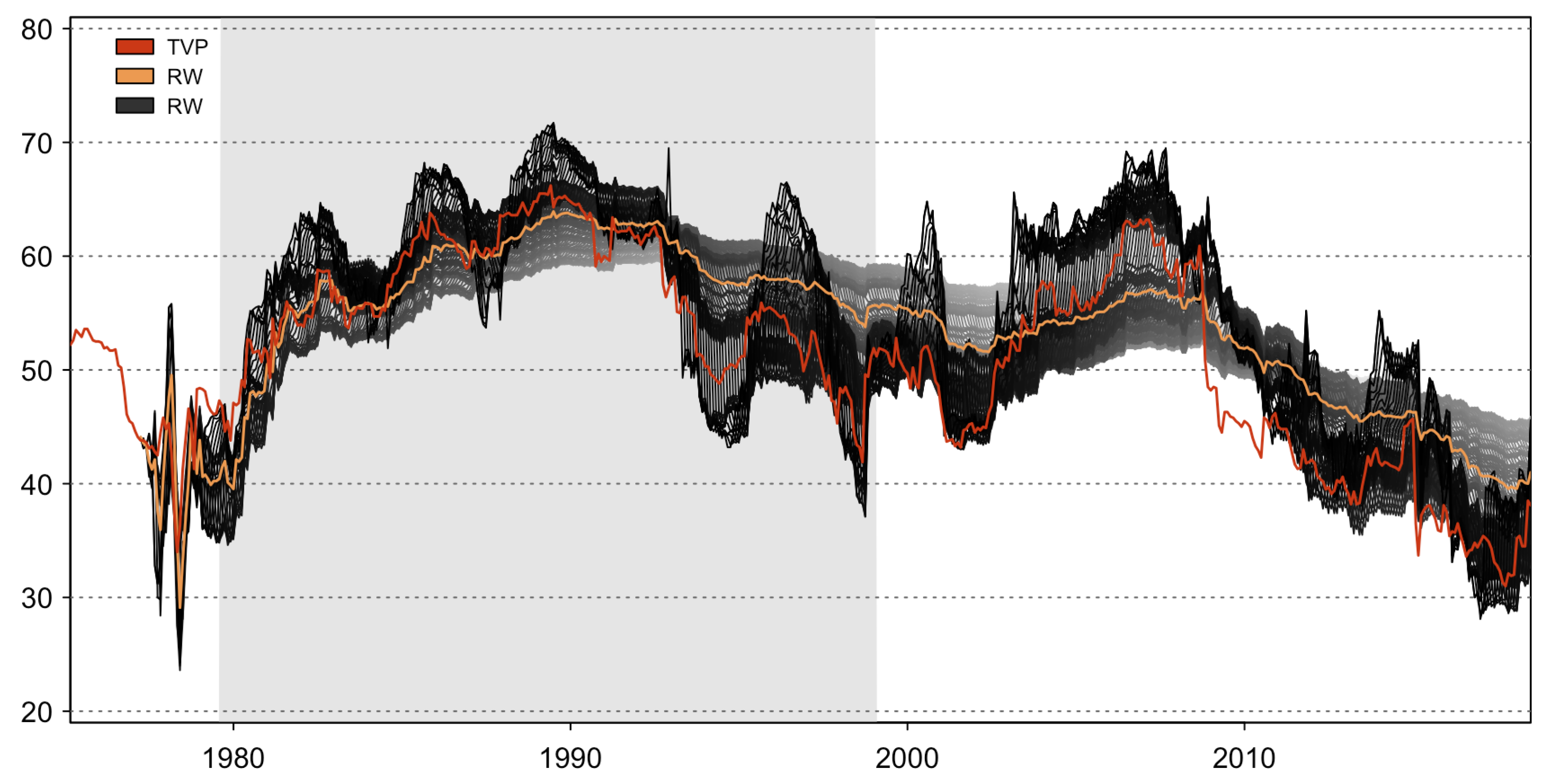
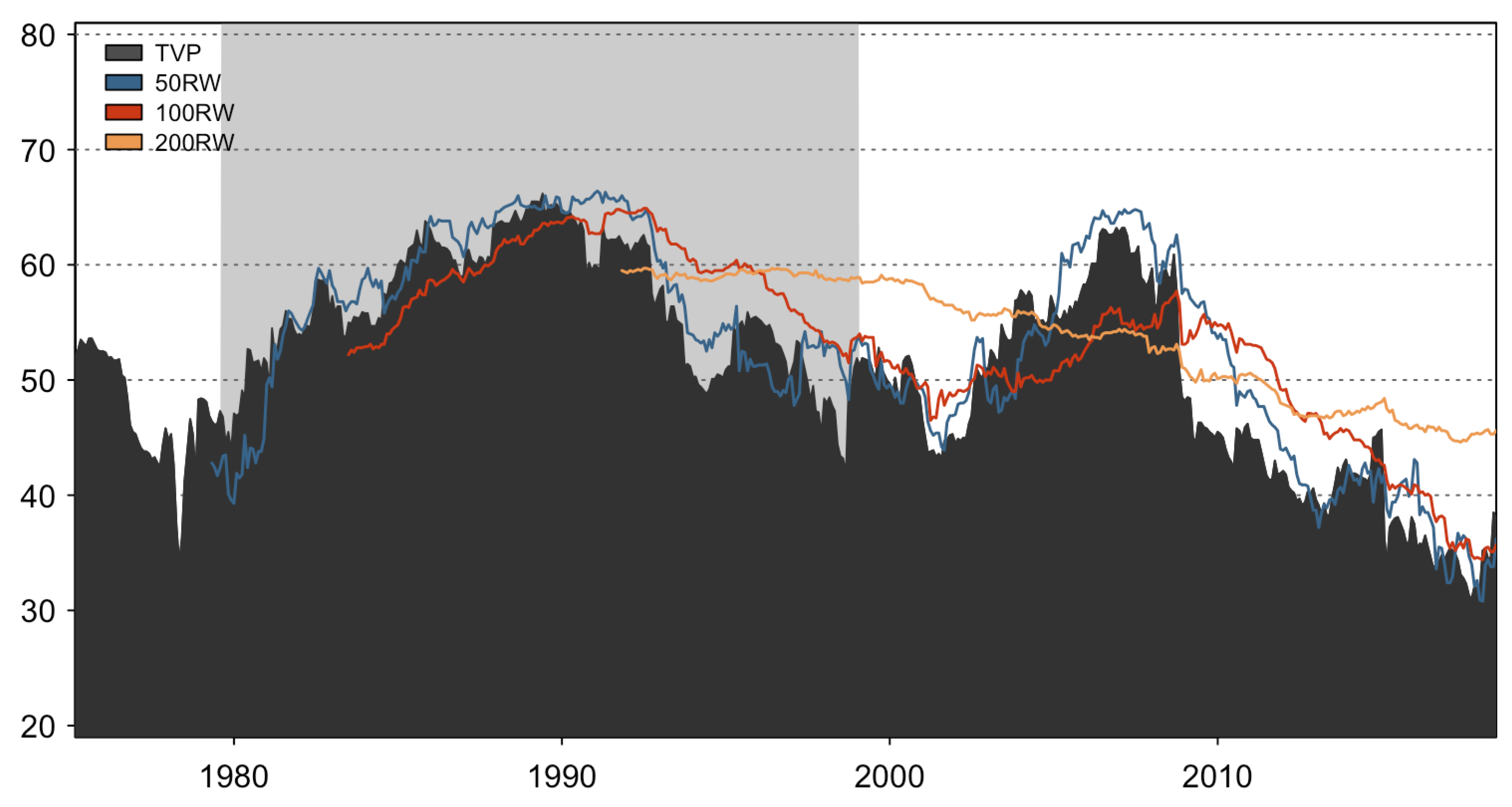
5.1. Dynamic Total Connectedness

We begin by presenting results for Dynamic Total Connectedness measures. These results are illustrated in Figure 5. More particularly, we consider the dynamic total connectedness of 50 different VAR models separated by virtue of window-length (i.e., 25, 30, …, 265, 270), their mean values, as well as results from the TVP-VAR. Interestingly, the mean of all rolling-window VARs’ dynamic total connectedness measures are similar to the results of the TVP-VAR. Furthermore, it is shown that the window size strongly influences the results of the dynamic total connectedness. the smaller the window size, the more volatile the results, whereas a large window size flattens out the dynamics over time.

Then, in the interests of comparison, we choose three window sizes and compare their results to the TVP-VAR. According to Figure 6, it seems as if a 100-month rolling-window size exhibits similar behaviour to that provided by the TVP-VAR model. In addition, we choose the 50-month and the 200-month rolling-window VAR models.

In Figure 7, we present the dynamic total connectedness measures of our proposed TVP-VAR approach, along with those based on the traditional rolling-window VAR methodology. It can be observed that the dynamic total connectedness based on the TVP-VAR adjusts immediately to events, and even faster than the smallest window-sized rolling window VAR, as evidenced by (i) the increase in 1992 and (ii) the decrease in 2009. Moreover, it should be mentioned that the 200-month rolling-window VAR drops nearly 40% of the observations and flattens out all dynamics. It even absorbs the effect the Great Recession had on the exchange rate market.

On a final note, despite that the overriding goal of the study is not to focus on the underlying story of our application, but rather, to emphasize the merits of the TVP-VAR connectedness approach, we should not lose sight of the fact that connectedness across the variables of our network increases during turbulent periods. In line with what we mentioned earlier, regarding the efforts of researchers to identify the relevant mechanisms that come into play during a crisis, our study provides new evidence that rather supports the idea that the foreign exchange market is very closely related (e.g., internationalization of the banking system) and that in the light of a financial crisis, developments in one currency might very well influence developments in another currency.

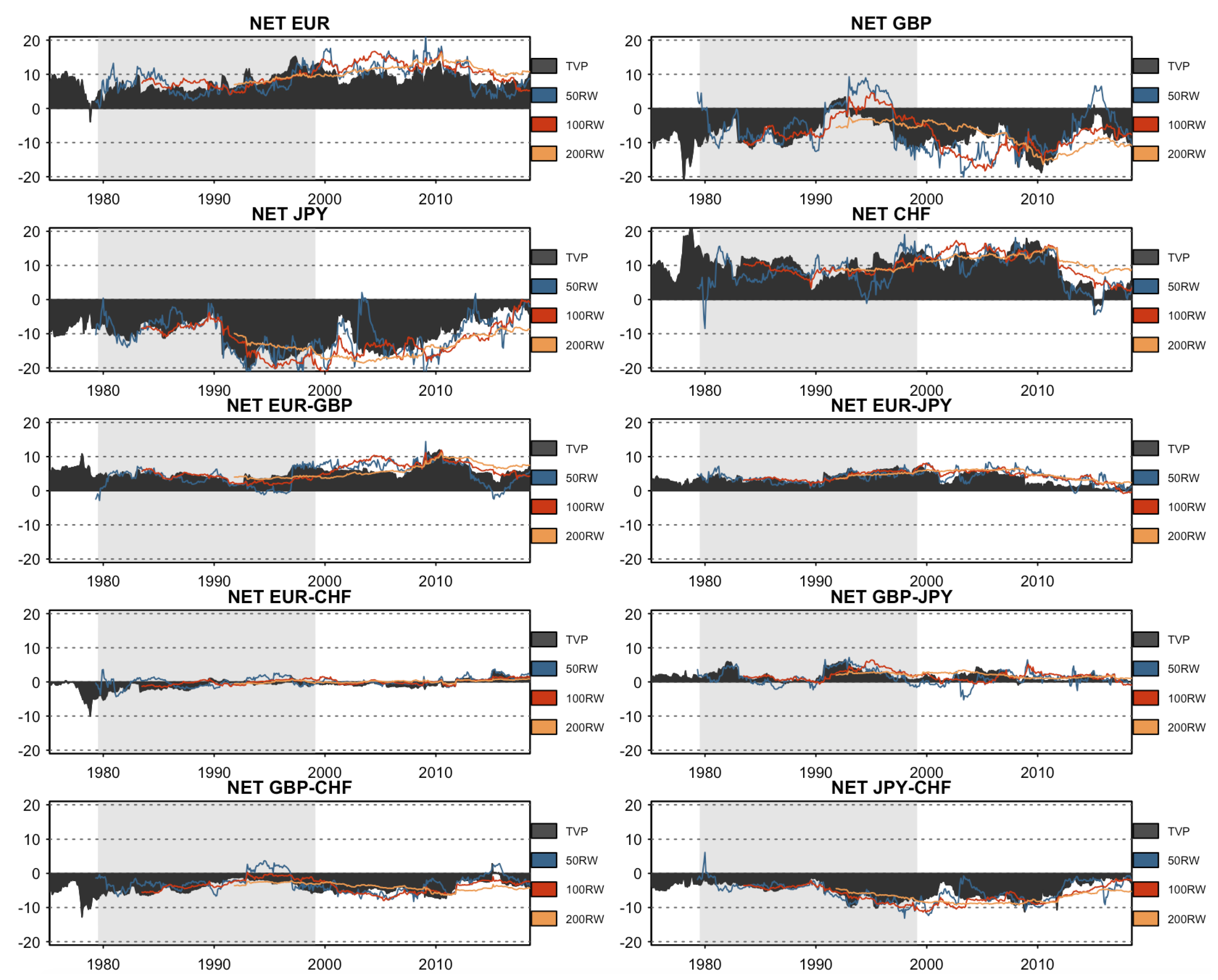
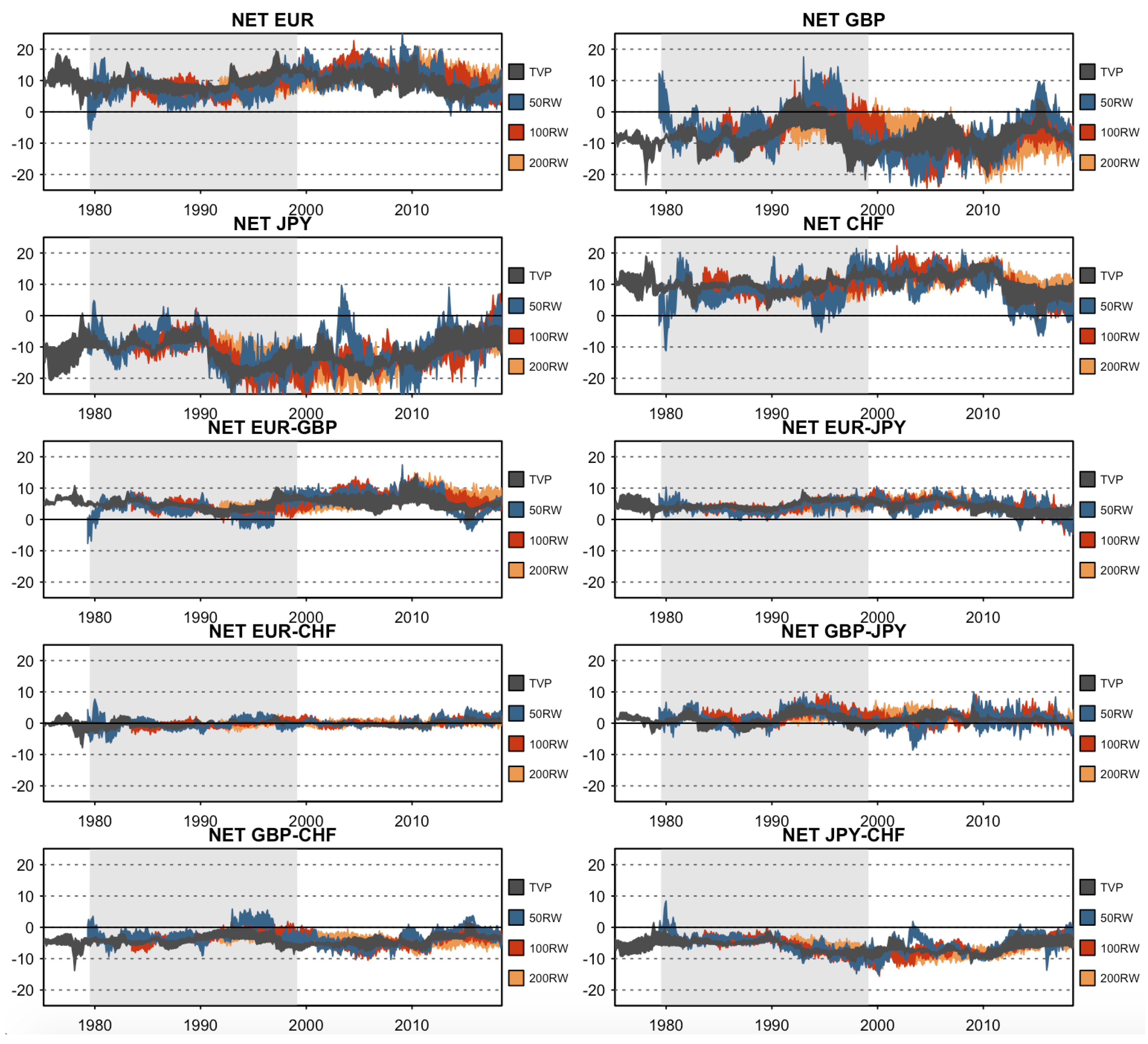
5.2. Net Total and Net Pairwise Directional Connectedness

We then turn to net total and net pairwise results, in order to (i) distinguish between net transmitters and net receivers of shocks in the foreign exchange market, and (ii) to specify the exact position between any given pair within our network of variables. We start with net total results and Figure 8. In Figure 8, a similar pattern is observed, in the sense that the net connectedness measures based on the smallest (largest) rolling-window size overreact (underreact) to dynamics. In comparison with Figure 7, it becomes clearer that the smallest rolling-window VAR overreacts to changes over time, as it can be seen in the net total connectedness plot of GBP, JPY, and CHF. We can observe that in the case of the GBP, the smallest rolling-window VAR deviates substantially from all others in 1980, from 1990 to 1995, and in 2012; in the case of the JPY, it deviates strongly around 2004 and 2012; while with respect to the CHF, we can see large deviations from 1980 until 1985, from 1992 until 1996, and again in 2012. Focusing on the upper part of Figure 8, it is quite evident that both EUR/USD and CHF/USD are persistent net transmitters of shocks in the foreign exchange market, while both GBP/USD and JPY/USD are persistent net receivers of shocks. With regard to the net pairwise directional connectedness results, the smallest window also appears to be the most volatile one. By contrast, the largest window size flattens out the net total connectedness dynamics. For example, if we focus on the EUR, we see a constant increase from 1990 to 2010 excluding all the adjustments within, while in the case of the GBP, it predicts approximately half of the influence of all others between 1998 and 2007. Once more, it seems that the middle-sized rolling-window is the most appropriate, even if it partially faces some weaknesses as well, such as the small adjustment in the case of the GBP (i.e., where it adjusts very slowly compared to the TVP-VAR after 1998). In other words, it seems that the TVP-VAR has the flexibility of the smallest rolling-window VAR model. All these observations hold, both for the total net and the net pairwise results.

It is interesting that the EUR and the CHF both dominate the GBP and the JPY, whereas the GBP dominates the JPY, both in 1990 when the Japanese financial crisis occurred, and between 2007–2010 when the Great Recession emerged. the bilateral relationship between the EUR and CHF is also interesting since it seems that both are influencing each other by the same amount, and hence, no one is driving the other, even if the co-movement between those two is the highest across all exchange rates of the study.

Even though the dynamics between rolling-window VARs and TVP-VAR models differ, all models came up with similar static connectedness measures, as shown in

Table 3. Dynamic connectedness table.

TVP-VAR
TO (i)	EUR	GBP	JPY	CHF	FROM (i)
EUR	40.1	18.2	10.9	30.8	59.9
GBP	23.8	48.3	7.4	20.5	51.7
JPY	15.1	9.0	57.5	18.3	42.5
CHF	30.7	16.3	12.5	40.5	59.5
Contribution TO others	69.5	43.6	30.9	69.6	213.6
NET directional connectedness	9.6	-8.1	−11.6	10.1	TCI
NPSO transmitter	2	1	0	3	53.4
50-Month Rolling-Window VAR
EUR	40.0	19.8	9.9	30.2	60.0
GBP	24.6	47.4	7.6	20.5	52.6
JPY	13.9	8.9	60.0	17.3	40.0
CHF	30.3	17.5	11.8	40.4	59.6
Contribution TO others	68.7	46.2	29.3	68.0	TCI
NET directional connectedness	8.8	-6.4	−10.7	8.4	53.0
NPDC transmitter	3	1	0	2
100-month Rolling-Window VAR
EUR	39.8	20.0	9.1	31.2	60.2
GBP	25.7	46.4	6.5	21.4	53.6
JPY	13.3	8.2	60.6	17.8	39.4
CHF	31.2	17.8	11.3	39.7	60.3
Contribution TO others	70.2	46.0	26.9	70.4	TCI
NET directional connectedness	10.0	-7.6	−12.5	10.1	53.4
NPDC transmitter	3	1	0	2
200-Month Rolling-Window VAR
EUR	39.3	20.3	8.6	31.8	60.7
GBP	26.2	46.1	5.7	21.9	53.9
JPY	13.4	7.7	60.9	18.1	39.1
CHF	31.9	18.1	10.9	39.1	60.9
Contribution TO others	71.5	46.1	25.3	71.8	TCI
NET directional connectedness	10.8	-7.8	−13.9	10.9	53.7
NPDC transmitter	3	1	0	2

Notes: Values reported are variance decompositions based on different VAR specficiations. Variance decompositions are based on 12-months-ahead forecasts. In both periods, a VAR lag length of order 1 was selected by the BIC.

. All of them identified that the EUR and the CHF are the main transmitters of shocks, whereas the JPY is the main receiver of shocks, followed by the GBP.

The highest bilateral influence is between the EUR and the CHF, which seem to face symmetric shocks from each other. Even though there is barely no domination between the CHF and the EUR, all models indicate that the EUR is the main transmitter, since it dominates all others, followed by the CHF which dominates the GBP and the JPY, and finally, the GBP dominates the JPY.

5.3. Sensitivity Analysis

5.3.1. Prior Sensitivity Analysis

Furthermore, we conducted a prior sensitivity analysis to see by how much results differ depending on the employed prior assumptions. Hereby, we used one uninformative prior, one informative prior, and 500 random Minnesota priors. the uninformative prior is specified as follows: $vec\left({\mathit{A}}_0\right)\sim N(vec\left(\mathbf{0}\right),m^{-p}·\mathit{I})$ and ${\mathsf{\Sigma }}_0=Cov\left(\mathit{y}\right)$; for the informative prior we estimated a VAR estimation based on the first 100 months: $vec\left({\mathit{A}}_0\right)\sim N(vec\left({\mathit{A}}_{OLS}\right)$ and ${\mathsf{\Sigma }}_0={\mathsf{\Sigma }}_{OLS}$. Finally, the Minnesota priors are constructed as follows: $vec\left({\mathit{A}}_0\right)\sim N(vec\left(diag\left(U(m,-0.99,0.99)\right)\right),m^{-p}·\mathit{I})$ and ${\mathsf{\Sigma }}_0=Cov\left(\mathit{y}\right)$, where the coefficients of the first lag are randomly uniformly distributed and all the others are zero. This prior assumes that all exchange rates are following a univariate process which can range from being highly persistent or being a random walk process. Since the parameters are all in a range between $-0.99$ and $0.99$, no series can be non-stationary. the parameters were chosen randomly, and so we could analyze various settings of parameters which allowed us to see by how much the results varied. Our results are based on 500 randomly chosen Minnesota priors.

As we can see in Figure 9 and Figure 10, all priors are converging to very similar results after 50 observations (50 times updating parameters). This result is interesting, since it shows that after a finite amount of coefficient updates, the results are going to be very similar.

5.3.2. Forgetting Factor Sensitivity Analysis

In addition, this TVP-VAR model heavily relies on forgetting factors, which are often set to a fixed value, as in Koop and Korobilis (2014), whereas in Koop and Korobilis (2013) they were allowed to vary using an additional process. However, Koop and Korobilis (2013) also stressed that the additional computation burden of this process is questionable since the forecasting performance is not being improved. Hence, we make use of the same priors as discussed in Section 5.3.1, whereas in addition, we allow both forgetting factors (${\kappa }_1,{\kappa }_2$) to vary independently from each other between $0.96$ and $0.99$. Calculating dynamic connectedness measures by allowing the TVP-VAR forgetting factors and priors to vary randomly offers additional information about how stable our results are. In Figure 11 and Figure 12, we can see by how much the dynamic total connectedness, net total connectedness, and net pairwise directional connectedness vary in 95% of all cases. This allows us to interpret how significant our results are. Furthermore, we get additional information; for instance, that the GBP cannot be identified either as a transmitter or receiver of shocks in the period between 1990 and 1998.

Finally, this study also provides confidence intervals for the rolling-window VAR connectedness measures. Hereby, we estimate the bootstrapped confidence intervals for the GIRF on which the GFEVD is based on. This procedure is computationally very demanding, since in every rolling-window estimation step, 200 GFEVD are estimated. In addition, Figure 13 and Figure 14 illustrate the confidence intervals of the rolling-window VAR connectedness measures. We note that the TVP-VAR uncertainty measures mainly overlap with the small- and the medium-sized rolling-window VARs, and that they are the ones that move the closest together. In Figure 14, when we focus on the net total connectedness measures of the JPY, we can see that the smallest rolling-window VAR results deviate quite considerably from all the others. This could indicate that estimation results have been driven by an outlier, since all the other confidence intervals overlap. Given these intervals, we may now interpret whether exchange rates are a significant net transmitter/receiver or net pairwise transmitter/receiver of shocks, which improves the connectedness literature substantially. Based on the results presented in Figure 14, we can state that the EUR and the CHF are significant net transmitters of shocks throughout the period of analysis, whereas the GBP and the JPY are significant net receivers of shocks based on the estimation results of the TVP-VAR and the 100-month rolling-window VAR results. Furthermore, the EUR and the CHF significantly dominate the GBP and the JPY. the GBP acts as a significant net transmitter of shocks to the JPY from 1990 until 1997 and from 2002 until 2008. Finally, it seems that neither the EUR nor the CHF affect each other even though they exhibit the highest unconditional correlation.

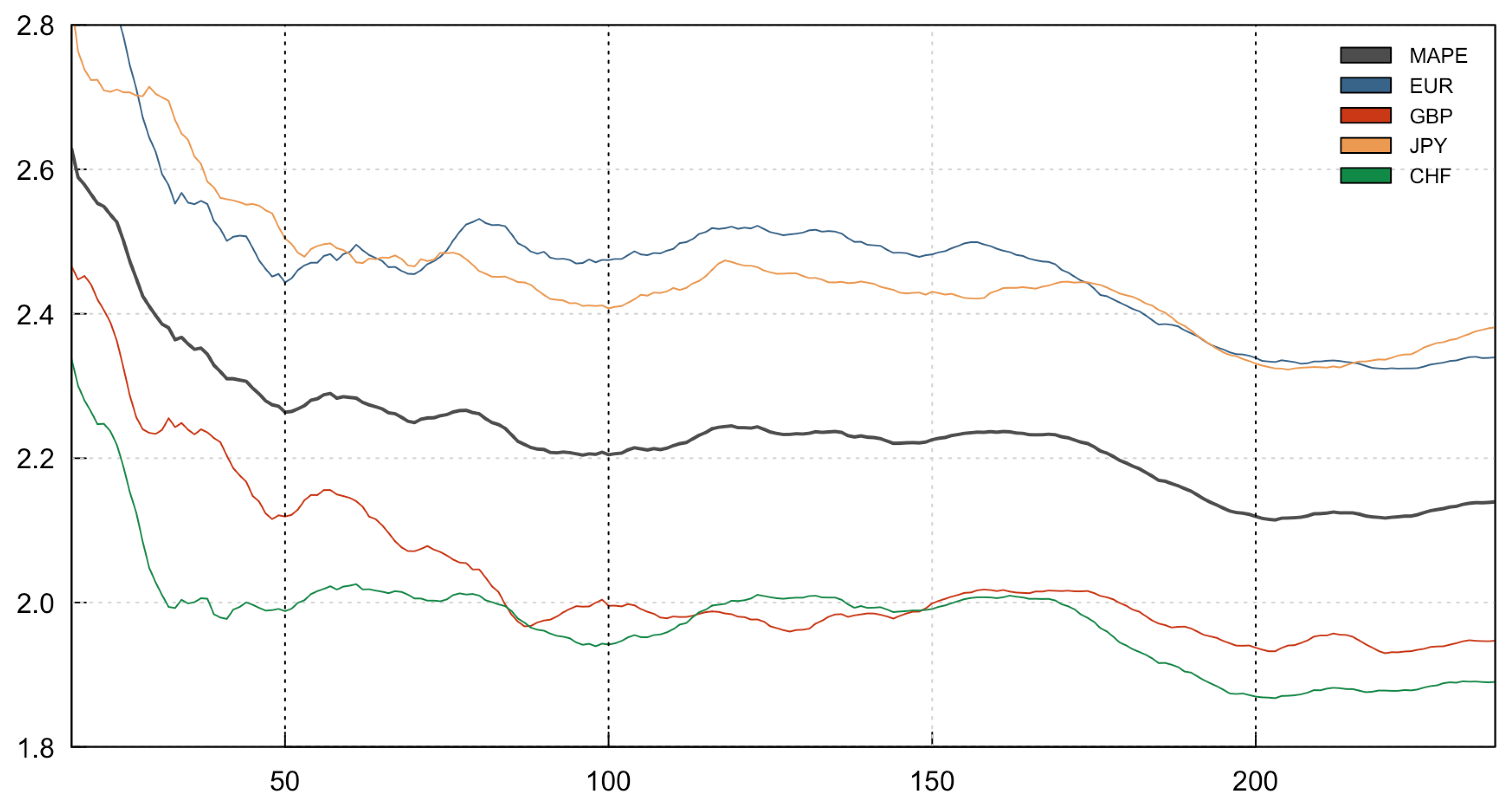
5.4. Forecast Performance

We also estimated forecasts for horizons up to one year ($H=1,2,3,6,9,12$) with a forecast evaluation period from January 1992 until January 2019. To evaluate the forecast performance, we utilized both the MAPE for each series and the average MAPE over all series. As shown in

Table 4. Forecast comparison using MAPE (I).

${\mathit{\kappa }}_1,{\mathit{\kappa }}_2$	EUR	GBP	JPY	CHF	$\overline{\mathit{MAPE}}$	EUR	GBP	JPY	CHF	$\overline{\mathbf{MAPE}}$
	1-Step Ahead Forecast					2-Step Ahead Forecast
0.99,0.99	$0.740$	$0.688$	$0.751$	$0.713$	$0.723$	$1.001$	$0.883$	$\mathbf{0.951}$	$0.935$	$0.943$
0.99,0.98	$0.739$	$0.686$	$0.751$	$0.711$	$0.722$	$1.000$	$0.881$	$\mathbf{0.951}$	$0.934$	$0.941$
0.99,0.97	$0.738$	$0.684$	$0.751$	$0.710$	$0.721$	$0.999$	$0.878$	$\mathbf{0.951}$	$0.933$	$0.940$
0.99,0.96	$\mathbf{0.737}$	$\mathbf{0.682}$	$\mathbf{0.750}$	$\mathbf{0.709}$	$\mathbf{0.720}$	$\mathbf{0.998}$	$\mathbf{0.876}$	$\mathbf{0.951}$	$\mathbf{0.932}$	$\mathbf{0.939}$
0.98,0.99	$0.746$	$0.688$	$0.757$	$0.721$	$0.728$	$1.010$	$0.888$	$0.956$	$0.940$	$0.949$
0.98,0.98	$0.745$	$0.687$	$0.757$	$0.720$	$0.727$	$1.008$	$0.885$	$0.956$	$0.939$	$0.947$
0.98,0.97	$0.743$	$0.686$	$0.757$	$0.719$	$0.726$	$1.006$	$0.882$	$0.955$	$0.938$	$0.945$
0.98,0.96	$0.742$	$0.684$	$0.756$	$0.719$	$0.725$	$1.004$	$0.881$	$0.954$	$0.938$	$0.944$
0.97,0.99	$0.756$	$0.687$	$0.763$	$0.727$	$0.733$	$1.025$	$0.893$	$0.962$	$0.946$	$0.956$
0.97,0.98	$0.754$	$0.686$	$0.763$	$0.726$	$0.732$	$1.021$	$0.890$	$0.962$	$0.944$	$0.954$
0.97,0.97	$0.752$	$0.686$	$0.762$	$0.725$	$0.731$	$1.018$	$0.889$	$0.961$	$0.943$	$0.952$
0.97,0.96	$0.751$	$0.685$	$0.760$	$0.725$	$0.730$	$1.015$	$0.887$	$0.960$	$0.942$	$\mathbf{0.951}$
0.96,0.99	$0.767$	$0.692$	$0.770$	$0.734$	$0.741$	$1.039$	$0.904$	$0.969$	$0.953$	$0.966$
0.96,0.98	$0.765$	$0.690$	$0.770$	$0.732$	$0.739$	$1.035$	$0.900$	$0.969$	$0.950$	$0.963$
0.96,0.97	$0.762$	$0.687$	$0.769$	$0.731$	$0.737$	$1.031$	$0.896$	$0.968$	$0.948$	$0.961$
0.96,0.96	$0.760$	$0.685$	$0.767$	$0.730$	$0.735$	$1.027$	$0.894$	$0.967$	$0.947$	$0.959$
RW 50	$0.779$	$0.713$	$0.782$	$0.752$	$0.757$	$1.057$	$0.932$	$0.994$	$0.974$	$0.989$
RW 100	$0.740$	$0.704$	$0.759$	$0.724$	$0.732$	$1.005$	$0.902$	$0.963$	$0.936$	$\mathbf{0.951}$
RW 200	$0.741$	$0.687$	$0.754$	$0.719$	$0.725$	$1.004$	$0.884$	$0.957$	$0.947$	$0.948$
	3-Step Ahead Forecast					6-Step Ahead Forecast
0.99,0.99	$1.208$	$1.036$	$\mathbf{1.143}$	$1.106$	$1.123$	$\mathbf{1.673}$	$1.424$	$1.639$	$\mathbf{1.453}$	$\mathbf{1.547}$
0.99,0.98	$1.208$	$1.034$	$1.144$	$1.105$	$1.122$	$\mathbf{1.673}$	$1.423$	$1.639$	$\mathbf{1.453}$	$\mathbf{1.547}$
0.99,0.97	$\mathbf{1.207}$	$1.031$	$\mathbf{1.143}$	$\mathbf{1.104}$	$1.122$	$\mathbf{1.673}$	$1.422$	$\mathbf{1.638}$	$\mathbf{1.453}$	$\mathbf{1.547}$
0.99,0.96	$\mathbf{1.207}$	$\mathbf{1.029}$	$\mathbf{1.143}$	$\mathbf{1.104}$	$\mathbf{1.121}$	$\mathbf{1.673}$	$\mathbf{1.421}$	$\mathbf{1.638}$	$1.454$	$\mathbf{1.547}$
0.98,0.99	$1.220$	$1.041$	$1.151$	$1.111$	$1.131$	$1.686$	$1.429$	$1.650$	$1.458$	$1.556$
0.98,0.98	$1.218$	$1.039$	$1.150$	$1.110$	$1.129$	$1.684$	$1.428$	$1.647$	$1.458$	$1.554$
0.98,0.97	$1.216$	$1.037$	$1.149$	$1.109$	$1.128$	$1.683$	$1.427$	$1.645$	$1.458$	$1.553$
0.98,0.96	$1.215$	$1.035$	$1.148$	$1.109$	$1.127$	$1.682$	$1.426$	$1.644$	$1.459$	$1.553$

and

Table 5. Forecast comparison using MAPE (II).

${\mathit{\kappa }}_1,{\mathit{\kappa }}_2$	EUR	GBP	JPY	CHF	$\overline{\mathbf{MAPE}}$	EUR	GBP	JPY	CHF	$\overline{\mathbf{MAPE}}$
	9-Step Ahead Forecast					12-Step Ahead Forecast
0.99,0.99	$\mathbf{2.032}$	$1.746$	$1.989$	$\mathbf{1.703}$	$\mathbf{1.867}$	$2.358$	$2.011$	$\mathbf{2.301}$	$\mathbf{1.917}$	$2.147$
0.99,0.98	$\mathbf{2.032}$	$1.744$	$1.988$	$1.704$	$\mathbf{1.867}$	$\mathbf{2.357}$	$2.009$	$\mathbf{2.301}$	$1.918$	$\mathbf{2.146}$
0.99,0.97	$\mathbf{2.032}$	$1.743$	$\mathbf{1.987}$	$1.705$	$\mathbf{1.867}$	$\mathbf{2.357}$	$2.007$	$\mathbf{2.301}$	$1.919$	$\mathbf{2.146}$
0.99,0.96	$\mathbf{2.032}$	$\mathbf{1.742}$	$1.988$	$1.706$	$\mathbf{1.867}$	$\mathbf{2.357}$	$\mathbf{2.005}$	$\mathbf{2.301}$	$1.920$	$\mathbf{2.146}$
0.98,0.99	$2.047$	$1.755$	$1.999$	$1.708$	$1.877$	$2.374$	$2.026$	$2.309$	$1.925$	$2.158$
0.98,0.98	$2.045$	$1.753$	$1.996$	$1.709$	$1.876$	$2.372$	$2.022$	$2.307$	$1.925$	$2.157$
0.98,0.97	$2.044$	$1.751$	$1.995$	$1.710$	$1.875$	$2.371$	$2.018$	$2.307$	$1.926$	$2.156$
0.98,0.96	$2.043$	$1.749$	$1.994$	$1.711$	$1.874$	$2.370$	$2.015$	$2.307$	$1.927$	$2.155$
0.97,0.99	$2.062$	$1.770$	$2.011$	$1.712$	$1.889$	$2.392$	$2.045$	$2.320$	$1.930$	$2.172$
0.97,0.98	$2.059$	$1.765$	$2.007$	$1.711$	$1.885$	$2.389$	$2.038$	$2.317$	$1.930$	$2.168$
0.97,0.97	$2.056$	$1.762$	$2.004$	$1.711$	$1.883$	$2.386$	$2.033$	$2.315$	$1.930$	$2.166$
0.97,0.96	$2.054$	$1.759$	$2.003$	$1.712$	$1.882$	$2.384$	$2.030$	$2.315$	$1.931$	$2.165$
0.96,0.99	$2.080$	$1.795$	$2.027$	$1.722$	$1.906$	$2.413$	$2.075$	$2.337$	$1.943$	$2.192$
0.96,0.98	$2.073$	$1.785$	$2.020$	$1.718$	$1.899$	$2.406$	$2.063$	$2.329$	$1.939$	$2.184$
0.96,0.97	$2.069$	$1.779$	$2.016$	$1.716$	$1.895$	$2.402$	$2.055$	$2.326$	$1.937$	$2.180$
0.96,0.96	$2.066$	$1.775$	$2.015$	$1.715$	$1.893$	$2.399$	$2.049$	$2.326$	$1.936$	$2.177$
RW 50	$2.170$	$1.940$	$2.137$	$1.815$	$2.016$	$2.546$	$2.284$	$2.518$	$2.078$	$2.357$
RW 100	$2.111$	$1.775$	$2.032$	$1.754$	$1.918$	$2.487$	$2.050$	$2.353$	$1.996$	$2.222$
RW 200	$2.045$	$1.749$	$2.005$	$1.732$	$1.883$	$2.375$	$2.018$	$2.316$	$1.948$	$2.164$

, the TVP-VAR models constantly outperform the rolling-window VAR models. Furthermore, we observe that TVP-VAR models with ${\kappa }_1=0.99$ are nearly always among the best models throughout the forecast horizons.

6. Conclusions

In this study, we introduced a TVP-VAR-based dynamic connectedness approach. In particular, this study constitutes a more detailed and complete illustration of the analysis provided by Antonakakis and Gabauer (2017), as three rolling-window sizes have been chosen based upon the mean absolute prediction error, which is better than just an arbitrarily chosen window size as in the original paper. Furthermore, we have provided a prior sensitivity analysis, uncertainty intervals for all connectedness measures, and finally, have evaluated the forecasting performance of the suggested approach. All of the above further strengthen the argument in favor of TVP-VAR-generated connectedness measures. On general principles, our approach can be regarded as an extension and improvement of the standard rolling-window VAR connectedness approach introduced by Diebold and Yılmaz (2014). To be more explicit, this extension improves the Diebold and Yılmaz (2014) method in four specific ways: (i) it allows for capturing possible changes in the parameters more accurately than in the rolling-window VAR specification; (ii) it is not as outlier-sensitive as the traditional rolling-windows approach; (iii) there is no need to arbitrarily set the rolling-window size; and (iv) there is no loss of observations in the calculation of the dynamic measures.

In order to provide evidence that TVP-VAR-generated measures of connectedness outperform their rolling-window counterparts, we began by constructing 50 different indices of dynamic total connectedness (i.e., based on the respective window length) and by comparing these indices to the results obtained by the TVP-VAR-generated connectedness approach. We noted that the TVP-VAR version of the index adjusted immediately to events, while adjustment was faster even when we compared against the shortest size of the rolling-window approach. We then turned to net total and net pairwise connectedness indices. In this case, we noted that indices based on the smallest rolling-window length tended to overreact across time and be more volatile, whereas indices based on the largest rolling-window length tended to flatten out connectedness dynamics. Again, TVP-VAR-generated indices tended to adjust quicker and be more flexible in responding to economic events.

Since estimating a TVP-VAR model requires a prior, we conducted a prior sensitivity analysis using one uninformative, one informative, and 500 randomly chosen Minnesota priors. In addition, we allowed both forgetting factors to vary randomly and independently from each other between 0.96 and 0.99 in order to deduce how much results are influenced by the choice of the forgetting factors. Findings in connection with the prior sensitivity analysis have shown that the influence of the prior is negligible after updating the coefficients approximately 50 times, whereas the forgetting factor sensitivity analysis provides information about the significance of the estimated results. In turn, we constructed bootstrapped confidence intervals for the rolling-window VAR-based approach, in order to be able to identify whether these connectedness measures were significant or not. On a final note, we evaluated the forecasting performance of both the rolling-window VAR and the TVP-VAR model and provided evidence that the TVP-VAR models constantly outperform the rolling-window VAR model, and that TVP-VAR models with a ${\kappa }_1=0.99$ in particular perform relatively better.

As far as the underlying narrative is concerned, the empirical investigation of the foreign exchange rate transmission mechanism revealed that the EUR and the CHF are the main transmitters of shocks throughout the period of analysis, whereas the GBP and the JPY are significant receivers of shocks. Furthermore, the EUR and the CHF significantly dominated the GBP and the JPY, whereas the JPY was driven by the GBP between 1990–1997 and 2002–2008. In addition, we found that neither the EUR nor the CHF transmitted shocks to one another.

References

1. Alter, Adrian, and Andreas Beyer. 2014. The Dynamics of Spillover Effects during the European Sovereign Debt Turmoil. Journal of Banking and Finance 42: 134–53. [Google Scholar] [CrossRef] [Green Version]
2. Anscombe, Francis J., and William J. Glynn. 1983. Distribution of the Kurtosis Statistic B2 for Normal Samples. Biometrika 70: 227–34. [Google Scholar] [CrossRef]
3. Antonakakis, Nikolaos, and David Gabauer. 2017. Refined Measures of Dynamic Connectedness Based On TVP-VAR. Technical Report. Munich: University Library of Munich. [Google Scholar]
4. Antonakakis, Nikolaos, Ioannis Chatziantoniou, and David Gabauer. 2019. Cryptocurrency Market Contagion: Market Uncertainty, Market Complexity, and Dynamic Portfolios. Journal of International Financial Markets, Institutions and Money 61: 37–51. [Google Scholar] [CrossRef] [Green Version]
5. Antonakakis, Nikolaos, David Gabauer, Rangan Gupta, and Vasilios Plakandaras. 2018. Dynamic Connectedness of Uncertainty across Developed Economies: A Time-Varying Approach. Economics Letters 166: 63–75. [Google Scholar] [CrossRef] [Green Version]
6. Antonakakis, Nikolaos, David Gabauer, and Rangan Gupta. 2019a. Greek Economic Policy Uncertainty: Does it Matter for Europe? Evidence from a Dynamic Connectedness Decomposition Approach. Physica A: Statistical Mechanics and Its Applications 535: 122280. [Google Scholar] [CrossRef]
7. Antonakakis, Nikolaos, David Gabauer, and Rangan Gupta. 2019b. International Monetary Policy Spillovers Evidence from A Time-Varying Parameter Vector Autoregression. International Review of Financial Analysis 65: 101382. [Google Scholar] [CrossRef]
8. Antonakakis, Nikolaos. 2012. Exchange Return Co-movements and Volatility Spillovers before and after the Introduction of Euro. Journal of International Financial Markets, Institutions and Money 22: 1091–109. [Google Scholar] [CrossRef] [Green Version]
9. Awartani, Basel, and Aktham Issa Maghyereh. 2013. Dynamic Spillovers Between Oil and Stock Markets in the Gulf Cooperation Council Countries. Energy Economics 36: 28–42. [Google Scholar] [CrossRef]
10. Baruník, Jozef, Evžen Kočenda, and Lukáš Vácha. 2016. Asymmetric Connectedness On the U.S. Stock Market: Bad and Good Volatility Spillovers. Journal of Financial Markets 27: 55–78. [Google Scholar] [CrossRef]
11. Baruník, Jozef, and Tomáš Křehlík. 2018. Measuring the Frequency Dynamics of Financial Connectedness and Systemic Risk. Journal of Financial Econometrics 16: 271–96. [Google Scholar] [CrossRef]
12. Baruník, Jozef, Evžen Kočenda, and Lukáš Vácha. 2017. Asymmetric Volatility Connectedness On the Forex Market. Journal of International Money and Finance 77: 39–56. [Google Scholar] [CrossRef] [Green Version]
13. Bekaert, Geert, Michael Ehrmann, Marcel Fratzscher, and Arnaud Mehl. 2014. The Global Crisis and Equity Market Contagion. Journal of Finance 69: 2597–649. [Google Scholar] [CrossRef] [Green Version]
14. Bubák, Vít, Evzen Kocenda, and Filip Zikes. 2011. Volatility Transmission in Emerging European Foreign Exchange Markets. Journal of Banking and Finance 35: 2829–41. [Google Scholar] [CrossRef] [Green Version]
15. Chatziantoniou, Ioannis, and David Gabauer. 2019. EMU-Risk Synchronisation and Financial Fragility Through the Prism of Dynamic Connectedness. Working Papers in Economics and Finance. Portsmouth: University of Portsmouth, Portsmouth Business School, Economics and Finance Subject Group. [Google Scholar]
16. Cogley, Timothy, and Thomas J Sargent. 2005. Drifts and Volatilities: Monetary Policies and Outcomes in the Post WWII US. Review of Economic Dynamics 8: 262–302. [Google Scholar] [CrossRef] [Green Version]
17. D’Agostino, Ralph B. 1970. Transformation to Normality of the Null Distribution of G1. Biometrika 57: 679–81. [Google Scholar]
18. Del Negro, Marco, and Giorgio E Primiceri. 2015. Time Varying Structural Vector Autoregressions and Monetary Policy: A Corrigendum. Review of Economic Studies 82: 1342–45. [Google Scholar] [CrossRef] [Green Version]
19. Diebold, Francis X., and Kamil Yilmaz. 2015. Trans-Atlantic Equity Volatility Connectedness: U.S. and European Financial Institutions, 2004–2014. Journal of Financial Econometrics 14: 81–127. [Google Scholar] [CrossRef] [Green Version]
20. Diebold, Francis X., and Kamil Yılmaz. 2009. Measuring Financial Asset Return and Volatility Spillovers, with Application to Global Equity Markets. Economic Journal 119: 158–71. [Google Scholar] [CrossRef] [Green Version]
21. Diebold, Francis X., and Kamil Yılmaz. 2012. Better to Give Than to Receive: Predictive Directional Measurement of Volatility Spillovers. International Journal of Forecasting 28: 57–66. [Google Scholar] [CrossRef] [Green Version]
22. Diebold, Francis X., and Kamil Yılmaz. 2014. On the Network Topology of Variance Decompositions: Measuring the Connectedness of Financial Firms. Journal of Econometrics 182: 119–34. [Google Scholar] [CrossRef] [Green Version]
23. Fisher, Thomas J., and Colin M Gallagher. 2012. New weighted portmanteau statistics for time series goodness of fit testing. Journal of the American Statistical Association 107: 777–87. [Google Scholar] [CrossRef]
24. Gabauer, David, and Rangan Gupta. 2018. On the Transmission Mechanism of Country-Specific and International Economic Uncertainty Spillovers: Evidence From A TVP-VAR Connectedness Decomposition Approach. Economics Letters 171: 63–71. [Google Scholar] [CrossRef] [Green Version]
25. Geraci, Marco Valerio, and Jean-Yves Gnabo. 2018. Measuring Interconnectedness Between Financial Institutions with Bayesian Time-Varying Vector Autoregressions. Journal of Financial and Quantitative Analysis 53: 1–20. [Google Scholar] [CrossRef] [Green Version]
26. Jarque, Carlos M., and Anil K. Bera. 1980. Efficient Tests for Normality, Homoscedasticity and Serial Independence of Regression Residuals. Economics Letters 6: 255–59. [Google Scholar] [CrossRef]
27. Kilian, Lutz. 1998. Small-Sample Confidence Intervals for Impulse Response Functions. Review of Economics and Statistics 80: 218–30. [Google Scholar] [CrossRef]
28. Kilian, Lutz. 1999. Finite-Sample Properties of Percentile and Percentile-t Bootstrap Confidence Intervals for Impulse Responses. Review of Economics and Statistics 81: 652–60. [Google Scholar] [CrossRef]
29. Koop, Gary, and Dimitris Korobilis. 2013. Large Time-Varying Parameter VARs. Journal of Econometrics 177: 185–98. [Google Scholar] [CrossRef] [Green Version]
30. Koop, Gary, and Dimitris Korobilis. 2014. A New Index of Financial Conditions. European Economic Review 71: 101–116. [Google Scholar] [CrossRef] [Green Version]
31. Koop, Gary, M. Hashem Pesaran, and Simon M. Potter. 1996. Impulse Response Analysis in Nonlinear Multivariate Models. Journal of Econometrics 74: 119–47. [Google Scholar] [CrossRef]
32. Korobilis, Dimitris, and Kamil Yilmaz. 2018. SSRN Electronic Journal. [CrossRef] [Green Version]
33. Lütkepohl, Helmut, Anna Staszewska-Bystrova, and Peter Winker. 2015. Comparison of Methods for Constructing Joint Confidence Bands for Impulse Response Functions. International Journal of Forecasting 31: 782–98. [Google Scholar] [CrossRef] [Green Version]
34. McMillan, David G., and Alan E. H. Speight. 2010. Return and Volatility Spillovers in Three Euro Exchange Rates. Journal of Economics and Business 62: 79–93. [Google Scholar] [CrossRef]
35. Pesaran, H. Hashem, and Yongcheol Shin. 1998. Generalized Impulse Response Analysis in Linear Multivariate Models. Economics Letters 58: 17–29. [Google Scholar] [CrossRef]
36. Petrova, Katerina. 2019. A Quasi-Bayesian Local Likelihood Approach to Time Varying Parameter VAR Models. Journal of Econometrics 212: 286–306. [Google Scholar] [CrossRef]
37. Primiceri, Giorgio E. 2005. Time Varying Structural Vector Autoregressions and Monetary Policy. Review of Economic Studies 72: 821–52. [Google Scholar] [CrossRef]
38. Reinhart, Carmen M., and Kenneth S. Rogoff. 2008. Is the 2007 US Sub-Prime Financial Crisis so Different? An International Historical Comparison. American Economic Review 98: 339–44. [Google Scholar] [CrossRef] [Green Version]
39. Stock, James H., Graham Elliott, and Thomas J. Rothenberg. 1996. Efficient Tests for an Autoregressive Unit Root. Econometrica 64: 813–36. [Google Scholar]
1.
Although there is in fact a wealth of literature regarding TVP-VAR models (see, inter alia, Primiceri 2005; Cogley and Sargent 2005; Koop and Korobilis 2013, 2014; Del Negro and Primiceri 2015; Petrova 2019) we do not focus on the TVP-VAR framework specifically, but we are rather concerned with utilising the TVP-VAR framework in order to improve the accuracy of the dynamic connectedness measures.
2.
Both the code for Monte Carlo simulation and the results of different rolling-windows are available upon request.
Figure 1. Monte Carlo simulation results with a single outlier.
Jrfm 13 00084 g001
Figure 2. Monte Carlo simulation results with a structural break.
Jrfm 13 00084 g002
Figure 3. Exchange rates.
Jrfm 13 00084 g003
Figure 4. Exchange rate returns.
Jrfm 13 00084 g004
Figure 5. Dynamic total connectedness. the darker the series, the smaller the window size, and vice versa (25, 26, …, 274, 275).
Jrfm 13 00084 g005
Figure 6. Mean absolute prediction error based on the 12-step-ahead forecast.
Jrfm 13 00084 g006
Figure 7. Dynamic total connectedness.
Jrfm 13 00084 g007
Figure 8. Net total and net pairwise directional connectedness measures.
Jrfm 13 00084 g008
Figure 9. Prior sensitivity analysis: Dynamic total connectedness.
Jrfm 13 00084 g009
Figure 10. Prior sensitivity analysis: Net total and net pairwise directional connectedness measures.
Jrfm 13 00084 g010
Figure 11. Dynamic total connectedness uncertainty.
Jrfm 13 00084 g011
Figure 12. Net total and net pairwise directional connectedness measures of uncertainty.
Jrfm 13 00084 g012
Figure 13. Confidence intervals: Dynamic total connectedness.
Jrfm 13 00084 g013
Figure 14. Confidence intervals: Net total and net pairwise directional connectedness measures of uncertainty.
Jrfm 13 00084 g014