The Impact of the COVID-19 Pandemic on the U.S. Economy: Evidence from the Stock Market


Research Institute of Economy, Trade and Industry, 1-3-1 Kasumigaseki, Chiyoda-ku, Tokyo 100-8901, Japan
J. Risk Financial Manag. 2020, 13(10), 233; https://0-doi-org.brum.beds.ac.uk/10.3390/jrfm13100233
Submission received: 25 August 2020
/
Revised: 28 September 2020
/
Accepted: 28 September 2020
/
Published: 1 October 2020
(This article belongs to the Special Issue COVID-19’s Risk Management and Its Impact on the Economy)
Abstract
:The coronavirus crisis has damaged the U.S. economy. This paper uses the stock returns of 125 sectors to investigate its impact. It decomposes returns into components driven by sector-specific factors and by macroeconomic factors. Idiosyncratic factors harmed industries such as airlines, aerospace, real estate, tourism, oil, brewers, retail apparel, and funerals. There are thus large swaths of the economy whose recovery depends not on the macroeconomic environment but on controlling the pandemic. Macroeconomic factors generated losses in industries such as production equipment, machinery, and electronic and electrical equipment. Thus, reviving capital goods spending requires not just an end to the pandemic but also a macroeconomic recovery.
1. Introduction
The COVID-19 pandemic has impacted the U.S. economy. Between January and July 2020, the unemployment rate rose from 3.6% to 10.1%, industrial production fell by 9%, and nonfarm employment fell by more than 12.5 million people.
The Federal Reserve (Fed) and federal and state governments have fought the downturn and the pandemic. Beginning in March, the Fed lowered the federal funds rate target by 150 basis points, provided forward guidance that interest rates would remain low, engaged in quantitative easing by buying Treasury and mortgage-backed securities, loaned to Treasury security primary dealers, backstopped money market funds, encouraged bank lending, and took other steps to maintain the flow of credit.1 Congress passed several pieces of legislation in March, including the Coronavirus Aid, Relief, and Economic Security Act (CARES). CARES provides loans for small businesses to continue paying wages (Paycheck Protection Program), expands unemployment benefits, pays USD 1200 per adult and USD 500 per child for individuals earning up to USD 75,000 (or USD 150,000 for taxpayers filing jointly), and channels funds to the health care system and to state and local governments. Several states and localities issued shelter-in-place (S-I-P) orders mandating that nonessential businesses close and that nonessential employees work from home. What are the mechanisms driving the economy’s response to the pandemic and to policy interventions?
Chetty et al. (2020) employed daily data to examine how spending, revenues, employment, and other variables responded at the county and industry level. Since the fall in GDP between 2019Q4 and 2020Q1 was driven by a drop in personal consumption expenditures, they investigated consumer spending. They reported that more than half of the drop in spending in June 2020 relative to June 2019 came from the top income quartile and only five percent of the drop came from the bottom quartile. They found that three-fourths of the drop in spending between the pre-coronavirus period and the middle of April came from goods and services requiring close contact such as hotels, transportation, and restaurant meals. They also found that high-income households reduced spending at businesses producing nontradables, causing these businesses to lay off low-income employees. CARES payments then stimulated spending by low-income individuals but did little to increase employment among the many laid off from jobs requiring close contact. The Paycheck Protection Program also did little to increase employment among these service workers. Chetty et al. concluded that stimulating aggregate demand and providing liquidity to businesses may not increase employment much when spending is constrained by health concerns.
Goolsbee and Syverson (2020) investigated whether the U.S. coronavirus-related downturn arose from S-I-P policies or from people choosing to refrain from activities to avoid infections. They employed cell phone data on customer visits to 2.25 million businesses in 110 industries. Comparing visits to contiguous locations with different S-I-P policies, they reported that legal shutdown orders explained only seven percentage points (ppts) of the 60 ppt drop in customer visits during the pandemic. They concluded that consumer actions to avoid infection rather than the lockdown policies were responsible for the lion’s share of the drop in spending across exposed businesses.
Eichenbaum et al. (2020a, 2020b, 2020c) calibrated how pandemics affect aggregate demand and aggregate supply. They modeled the interactions between agents’ economic decisions and the spread of the infection. They found that people avoiding infection risk caused labor supply and thus aggregate supply to fall and consumption and thus aggregate demand to drop. The simultaneous reduction in aggregate supply and aggregate demand in their model leads to a deep, persistent recession.
Larson and Sinclair (2020) and Aaronson et al. (2020) attempted to predict how the coronavirus crisis affected unemployment insurance (UI) claims in the U.S. Larson and Sinclair found that, including the dates when states declared a state of emergency due to COVID-19, a panel framework improved forecasts of initial UI claims over the 14 March to 16 May 2020 period. Aaronson et al. employed Google Trends data in an event study of seven large hurricanes to calculate the elasticity of UI claims with respect to the intensity of searches on the topic “unemployment”. They then used these elasticities to improve the out-of-sample forecasts of the increase in initial UI claims from two-hundred and fifty-thousand on 14 March 2020 to three million on 21 March and six million on 28 March.
This paper investigates how the pandemic and the associated policy actions have affected the U.S. economy by examining the response of sectoral stock prices. Finance theory indicates that stock prices equal the expected present value of future cash flows. They thus contain information about how investors expect firms and industries to be affected.
Previous research has investigated how the coronavirus crisis has affected asset prices. Ramelli and Wagner (2020) examined how COVID-19 affected U.S. stock returns. They used the capital asset pricing model and the Fama and French (1993, 2015) factors to adjust returns. They found that as news of the outbreak emerged between 20 January and 21 February 2020, adjusted returns on stocks of U.S. firms that traded with China fell more. Then, as concern about the crisis exploded over the 24 February to 20 March 2020 period, they reported that the adjusted returns on firms with less cash and higher leverage fell more.
Pagano et al. (2020) found that stocks of firms that are resilient to social distancing perform better than nonresilient stocks. They employed Koren and Pető’s (2020) affected share variable that measures the extent to which jobs can be done without close human contact. They classified firms as resilient if their affected share values were below the median and as not resilient if their affected share values were above the median. Over the 24 February–20 March 2020 period, they reported that capital asset pricing model-adjusted returns were 10% for the high-resilience portfolio and −15% for the low-resilience portfolio. The high-resilience portfolio thus outperformed the low-resilience portfolio by 25%. For returns adjusted using the Fama and French (1993, 2015) factors, they reported that the high-resilience portfolio outperformed the low-resilience portfolio by between 15% and 20%.
Chan and Marsh (2020) compared the drop in the Dow Jones Industrial Average (DJIA) from 21 February 2020 to the end of March 2020 with drops during other market crashes and pandemics. They reported that the DJIA fell about as much over their sample as it did at a comparable point during the 1929 Great Depression and much more than during previous pandemics such as the 1918 Spanish Flu epidemic. They attributed the large drop in 2020 to uncertainty about the technical characteristics of COVID-19, the effects of S-I-P policies on the economy, and the impact of the pandemic on global value chains.
Gormsen and Koijen (2020) employed dividend futures to measure the economic impact of the crisis. As of 9 June 2020, their model predicted a 2 ppt fall in U.S. GDP growth forecasted over the next year relative to forecasts on 1 January 2020, a 9 ppt fall in U.S. dividends, a 3.1 ppt fall over the next year relative to forecasts on 1 January 2020, a 3.1 ppt drop in European GDP growth, and a 14 ppt drop in European dividends. They stated that their approach might understate the falls because the macroeconomic changes in 2020 are large relative to historical experience.
Sharif et al. (2020) used the coherence wavelet method and wavelet-based Granger causality tests and daily data between 21 January 2020 and 30 March 2020 to investigate the relationship between the COVID-19 outbreak, the U.S. Dow Jones Index, the spot price of West Texas Intermediate (WTI) crude oil, and measures of economic uncertainty and geopolitical risk. They found that the U.S. stock market, economic uncertainty, and geopolitical risk are all affected by the twin shocks of the coronavirus and falling oil prices.
Gharib et al. (2020) used the bootstrap techniques of Phillips and Shi (2018) and daily data over the 4 January 2010 to 4 May 2020 period to investigate whether there are common bubbles between WTI oil prices and gold prices. They found that during the COVID-19 crisis these two series shared explosivity, with oil prices experiencing a negative bubble and stock prices experiencing a positive bubble. Granger causality tests indicated that there was bilateral contagion between the two markets. Their findings indicate that gold has been functioning as a safe haven asset during the pandemic.
Lyocsa et al. (2020) employed daily data over the 2 December 2019–30 April 2020 period to investigate the relationship between fear about COVID-19 and uncertainty in the U.S. S&P 500 and major stock market indices from nine other countries. They measured fear of the virus by examining Google searches for terms related to the virus and uncertainty by the daily variance of market returns. They reported that excess search volume predicts future stock market variance for every country examined.
Most of the previous work has investigated the relationship between the coronavirus crisis and stocks or other assets measured at a fairly aggregated level. The contribution of this paper is to investigate how the pandemic has affected U.S. stock returns in 125 sectors. Black (1987, p. 113) observed that, “The sector-by-sector behavior of stocks is useful in predicting sector-by-sector changes in output, profits, or investment. When stocks in a given sector go up, more often than not that sector will show a rise in sales, earnings, and outlays for plant and equipment”. This paper also decomposes cumulative returns into the portions driven by macroeconomic factors and by idiosyncratic factors. The results present evidence at a disaggregated level concerning how investors expect the pandemic and policy responses to affect the U.S. economy.
2. Materials and Methods
This paper considers stock returns for 125 sectors during the COVID-19 crisis. It focuses on the period beginning on 19 February 2020, when U.S. stock prices began falling, until 10 July 2020. The sectors examined are listed in column (1) of Table 1 and the values on 10 July of one dollar invested on 19 February are presented in column (2). This paper investigates how both the macroeconomic environment and sector-specific factors affect returns. Over the sample period, the coronavirus pandemic was a key event driving these responses.
To capture how the aggregate economic environment affects returns, several macroeconomic variables are used. The first is the return on the overall U.S. stock market, following a long tradition in finance of using the return on the market to control for economy-wide influences (see, e.g., Brown and Warner 1980, 1985). The second is the return on the world stock market, capturing how changes in the world economy influence sectoral returns. The third is the nominal effective exchange rate, following a body of research that investigates sectors’ exchange rate exposures (see, e.g., Dominguez and Tesar 2006). The fourth is the price of oil, reflecting the large impact of oil prices across U.S. sectors (see, e.g., Thorbecke 2019). The fifth is inflation, drawing on evidence that inflation is a state variable that matters for stock returns (see, e.g., Chen et al. 1986). The other three variables are interest rates or interest rate spreads, building on the large literature indicating that these affect equity risk premia (see, e.g., Aït-Sahalia et al. 2020). These last three variables are the change in the interest rate on three-month Treasury securities, the change in the spread between interest rates on ten-year and three-month Treasury security, and the change in the spread between interest rates on Moody’s seasoned Baa corporate bonds and ten-year Treasury securities.
Data on sectoral stock returns, the return on the U.S. aggregate stock market and the world stock market, and changes in the price of WTI crude oil come from the Datastream database. Data on changes in interest rates and interest rate spreads, changes in the breakeven inflation rate calculated from U.S. Treasury inflation-protected securities (TIPSs), and changes in the Federal Reserve broad trade-weighted exchange rate index come from the Federal Reserve Bank of St. Louis FRED database. The exchange rate data are available beginning in 2006, so the sample period extends from 4 January 2006 to 10 July 2020.2
Augmented Dickey–Fuller (ADF) tests on the 125 sectoral returns and the eight macro factors permit rejection in every case of the null hypothesis that the series have unit roots. Sectoral returns are thus regressed on the eight factors.
The estimated equations take the form:
where the data are daily and ∆Ri,t is the change in the log of the stock price index for sector i, ∆Rm,US,t is the change in the log of the price index for the U.S. aggregate stock market, ∆Rm,World,t is the change in the log of the price index for the world stock market, ∆ert is the change in the Federal Reserve broad trade-weighted exchange rate index, ∆Poil,t is the change in the log of the spot price for WTI crude oil, ∆Inftt is the change in the five-year breakeven inflation rate calculated from TIPS, ∆ithree,t is the change in the interest rate on three-month Treasury securities, ∆iten-three,t is the change in the spread between interest rates on ten-year and three-month Treasury security, and ∆ibaa-ten,t is the change in the spread between interest rates on Moody’s seasoned Baa corporate bonds and ten-year Treasury securities.3
Chen et al. (1986) and many others have regressed stock portfolio returns on macroeconomic variables. As in this paper, Chen et al.’s macroeconomic variables included variables related to inflation, oil prices, the overall stock market, the spread between returns on long- and short-term Treasury bonds, and the spread between returns on risky corporate bonds and long-term Treasury bonds. They argued that, while only physical shocks such as supernovas and earthquakes are truly exogenous, the economy-wide variables they employed can be taken as exogenous relative to portfolios of stocks. The same as the appearance of a supernova, the emergence of COVID-19 was exogenous. It impacted both macroeconomic variables (e.g., when the Fed lowered interest rates in response to the crisis) and sector-specific variables (e.g., when people stopped visiting casinos). Because this paper uses highly disaggregated sectoral data, the flow of causality from returns on individual sectors such as casinos to the economy-wide variables should be second-order relative to the flow of causality in the other direction. This paper thus follows Chen et al. in positing the causality flows from the macroeconomic variables on the right-hand side of Equation (1) to the sectoral returns on the left-hand side.
Equation (1) is a standard regression of simple returns on macroeconomic variables. The simple returns can then be compounded as in Table 1 to calculate the value on 10 July of one dollar invested on 19 February. The simple returns in Equation (1) can also be divided into the part driven by macroeconomic variables and the part driven by sector-specific factors. These two parts can each be compounded to find the value on 10 July of one dollar invested on 19 February driven by macroeconomic variables and by idiosyncratic factors. The COVID-19 pandemic and the stimulus in response to it have affected the macroeconomic environment and also impacted sectors in various ways. The decomposition sheds light on when economy-wide and when sector-specific influences are driving performance.
As a robustness test, the right-hand-side variables in Equation (1) are replaced by the five Fama and French factors. Fama and French (1993, 2015) reported that five common factors are useful for explaining the cross-section of stock returns. These factors are: (1) the return on the aggregate U.S. stock market index minus the return on one-month U.S. Treasury securities, (2) the average return on nine small capitalization stock portfolios minus the average return on nine large capitalization stock portfolios, (3) the average return on two high-book value to market value portfolios minus the average return on two low-book value to market value portfolios, (4) the average return on two robust operating profitability portfolios minus the average return on two weak operating profitability portfolios, and (5) the average return on two conservative investment portfolios minus the average return on two aggressive investment portfolios. Regressing sectoral returns on these five factors provides an alternative way of decomposing returns into systematic and idiosyncratic portions.
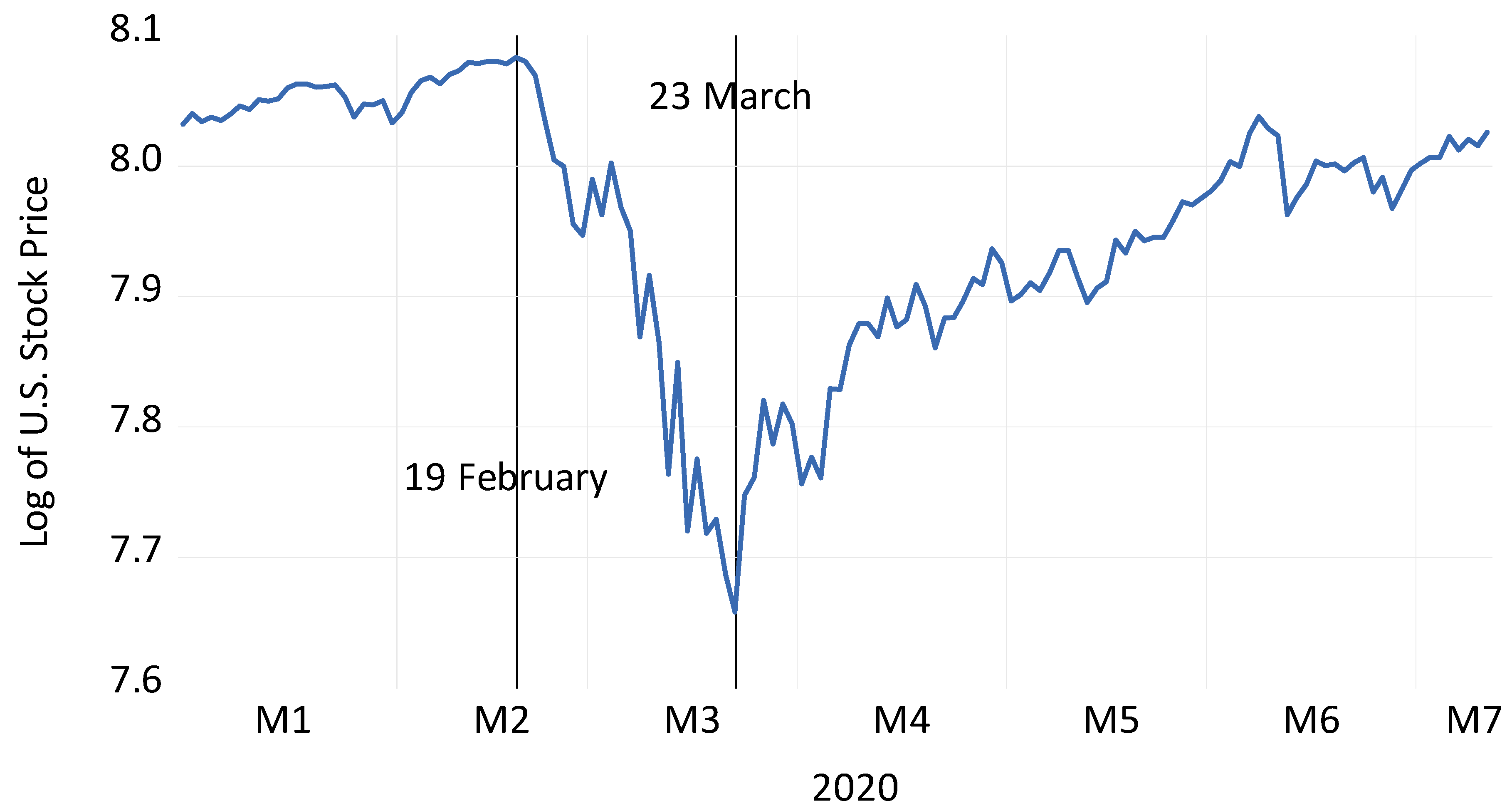
Figure 1 plots aggregate U.S. stock prices from 1 January 2020 to 10 July 2020. U.S. stock prices, after increasing between 1 January and 19 February, fell logarithmically by 42% between 19 February and 23 March. They then increased by 37% between 23 March and 10 July. Smith and Badkar (2020), Wells (2020), and others discussed how concerns about coronavirus starting on 19 February caused investors to sell U.S. stocks and move into safe-haven assets such as long-term Treasury securities and gold. The Fed then announced aggressive actions on 23 March to promote recovery (see Federal Reserve 2020). Hartley and Rebucci (2020), employing an event study methodology, found that the announcement caused a statistically significant decline of −0.16% in 10-year Treasury yields. Ramelli and Wagner (2020), finding a deleterious impact of low liquidity and high leverage on firm performance during the pandemic, reported that the Fed announcement weakened this effect. Chen et al. (2020), examining the mortgage-backed security (MBS) market, found that the relationship between MBS prices in the specified pool market and the to-be-announced market returned to normal only after the Fed’s announcement on 23 March. Ablan et al. (2020), considering the effect of news on asset prices, reported that news of the CARES stimulus package and the Fed’s aggressive actions led to the stock market rally that began after 23 March. Despite bad news in terms of infections, stock prices trended upwards between 23 March and 10 July. Fed actions, the CARES stimulus, and the possibility of future expansionary policies contributed to this rebound.
The focus in the next section is on sectoral performance over the 19 February 2020–10 July 2020 sample period. The sample period is also divided into the 19 February–23 March sub-sample when news about the virus itself impacted markets and the 23 March–10 July sub-sample when news of government stimulus helped to revive markets.
The variables in Equation (1) fluctuated over this period. World stock prices behaved the same as U.S. stock prices in Figure 1. After increasing between 1 January and 19 February, they fell logarithmically by 41% between 19 February and 23 March. They then increased by 33% between 23 March and 10 July. The trade-weighted exchange rate appreciated 8% between 19 February and 23 March and then depreciated by 6% between 23 March and 10 July. The breakeven inflation rate fell from 165 basis points on 19 February to 37 basis points on 23 March and then rose to 125 basis points on 10 July. Oil prices fell from USD 53 per barrel on 19 February to USD 20 per barrel on 23 March. They stayed fairly constant until mid-April, and then fell to negative USD 38 on 20 April. By 10 July, they had recovered to USD 40 per barrel. The three-month Treasury rate fell from 155 basis points on 19 February to almost zero on 23 March and remained close to zero until 10 July. The spread between the 10-year and three-month Treasury rates increased by 75 basis points between 19 February and 23 March and then fell by 25 basis points between 23 March and 10 July. The spread between the BAA corporate bond rate and the 10-year Treasury rate increased by 227 basis points between 19 February and 23 March and then fell 157 basis points between 23 March and 10 July.
3. Results
Table 2 presents the betas for the eight variables in Equation (1) and the adjusted R-squared. The adjusted R-squared across the 125 portfolios in column (10) averages 0.578. This indicates that the macroeconomic variables explain a substantial portion of the daily returns.
Column (2) reports assets’ exposure to the U.S. stock market. Real estate investment trusts (REITs), real estate, home construction, and real estate holdings and development are all highly exposed to the aggregate U.S. market. Banks, life insurance, and consumer lending also have large market betas. Tourism-related sectors such as airlines, hotels and motels, and recreational vehicles also have market exposures greater than 1.2. These are thus cyclically sensitive industries.
Other industries exhibit much less cyclical sensitivity in column (2). These include gold mining, brewers, distillers and vintners, and makers of food products, tobacco products, soft drinks, nondurable household products, consumer staples, and fruits and grains. Other sectors with low market betas are those related to health care (medical services, medical supplies, medical equipment, health care, pharmaceuticals, and drug retailers). Restaurants and bars and funerals also have market betas of 0.82 or less. Many of these sectors produce essential goods and demand for their products remains strong even during slowdowns.
Columns (3) and (4) report sectors’ exposure to world stock market returns and to U.S. dollar appreciations. Export-oriented sectors are exposed to these factors. For instance, several parts of the oil industry, which has recently become more export-oriented, are affected by the economic conditions in the rest of the world (as proxied by world stock market returns) and by exchange rates. These include oil equipment and services, crude oil production, international oil and gas, and oil refining and marketing. Metals such as iron and steel, copper, and gold mining are exposed to exchange rate appreciations. These are typically priced in U.S. dollars, and when the dollar appreciates the currencies of importing countries depreciate and importers are unable to purchase as much. Various producers of machinery and electronic goods are also exposed to slowdowns in the rest of the world.
Office, retail, and hotel and lodging REITs, specialty and apparel retailers, and providers of cable TV services, electronic entertainment, and nondurable household products are not exposed to the world stock market. These goods are nontradable and not sensitive to slowdowns on the rest of the world. Similarly, home improvement, diversified, and drug retailers, restaurants and bars, trucking, and other nontradables are less exposed to U.S. dollar appreciations.
Column (5) shows sectors’ sensitivities to oil price increases. Oil refining and marketing, crude oil production, international oil and gas, and pipelines benefit from higher oil prices. Several parts of the machinery sector, including engines, industrial machinery, and tools, also benefit from higher oil prices. Melek (2018) reported that, after the shale revolution, increased capital expenditures by oil producers triggered an increase in capital expenditures by nonoil producers. Higher oil prices that lead to greater investment by oil companies can thus benefit the machinery sector. The industrial transport sector that transports oil also benefits from higher oil prices. On the other hand, the automobile industry is harmed by higher oil prices.
Columns (6)–(9) indicate that the other variables also exert a variety of effects on industry portfolios. One notable finding is the impact of interest rates and interest rate spreads on the banking sector. They indicate that a 100 basis point increase in the three-month Treasury security rate or in the spread between the ten-year and the three-month Treasury rates would increase banks stock prices by between three and four percent. Banks accept short-term deposits and extend longer term loans. As Petralia et al. (2019) highlighted, banks profit from the spread between the interest rate they earn on long-term loans and the interest rate they pay on short-term deposits (the net interest margin). Petralia et al. also found that increases in the short-term Treasury interest rate and in the spread between the ten-year and three-month Treasury rates are positively related to the net interest margin. The fall in interest rates and interest rate spreads during the pandemic have thus harmed bank profitability.
Table 1 indicates how much one dollar invested at the beginning of the period would be worth at the end of the period. Numbers below one indicate that one dollar invested at the beginning of the period would have lost value and numbers above one indicate that it would have gained value. Columns (2)–(4) concern investments over the 19 February–10 July period, columns (5)–(7) investments over the 19 February–23 March period, and columns (8)–(10) investments over the 23 March–10 July period. For all three periods, the leftmost column presents results for the overall stock return in a sector, the middle column for the portion of the return driven by macroeconomic factors, and the rightmost column for the portion driven by idiosyncratic factors.
According to column (2), the worst performing sector in terms of overall stock returns over the 19 February–10 July period is airlines. One dollar invested on 19 February would be worth only 38 cents on 10 July. The closely related aerospace sector that provides planes to the airline sector has also suffered, with a dollar investment falling to 50 cents by the end of the period. Columns (3) and (4) indicate that the lion’s share of this fall has been driven by idiosyncratic rather than macroeconomic factors. The pandemic grounded flights and decimated these industries.
The next worst performing sectors in terms of overall returns are hotel and lodging REITs and real estate holding and development. One dollar invested on 19 February in hotel and lodging REITs would be worth only 39 cents on 10 July and one dollar invested in real estate holding and development would be worth only 41 cents. Columns (3) and (4) indicate that two-thirds of the drop was due to idiosyncratic factors and one-third to the macroenvironment. Investments in two related sectors, retail REITs and mortgage REITs, also lost more than half of their value over this period. The crisis restricted visits to hotels and retail stores and jeopardized agents’ ability to pay rents and mortgages. On the macroeconomic front, these sectors all have large exposures to the aggregate U.S. market and also to oil prices. The fall in U.S. stock prices and in oil prices thus contributed to the losses.
The oil sector has also performed poorly. One dollar invested in oil equipment and services on 19 February fell to 42 cents, one dollar in crude oil production fell to 45 cents, and one dollar in oil refining and marketing and in pipelines fell to 55 cents. Columns (3) and (4) indicate that both macroeconomic factors and idiosyncratic factors roiled the industry. Table 2 indicates that the oil sector is highly exposed to oil prices. The drop in oil prices contributed to losses in the oil industry. In addition, S-I-P policies and individuals’ reluctance to travel reduced oil demand. Brower (2020) reported that oil production in the U.S. fell by 30% during the crisis.
Tourism has been decimated. One dollar invested in casinos and gambling fell to 55 cents, one dollar in travel and tourism to 57 cents, and one dollar in hotels and motels to 58 cents. Macroeconomic factors contributed to these losses but idiosyncratic factors contributed more. Concern about infections and lockdowns have reduced cruise ship voyages, trips to crowded locations, and visits to hotels. In addition, these sectors all have betas to the U.S. stock market that exceed 1.12. The fall in U.S. stock prices thus contributed to these losses.
Recreational services such as fitness centers and also banks and consumer lending have suffered. One dollar invested in recreational services fell to 51 cents and one dollar invested in banks and consumer lending fell to 58 cents. Customers avoided fitness centers. Banks and consumer lending faced the danger that borrowers may be unable to repay loans. Noonan and Armstrong (2020) reported that U.S. banks set aside much more than expected for loan loss provisions in 2020Q2. In addition, Table 2 indicates that the banking sector is highly exposed to reductions in the three-month Treasury rate and the spread between the ten-year and the three-month Treasury rates. The Fed policy that led these two variables to fall thus reduced banks’ net interest margins and their profitability. Finally, credit card balances, a major profit source for banks, tumbled in 2020Q2 (Smith 2020).
Other sectors that performed badly are brewers, apparel retailers, radio and TV broadcasting, and funerals. The returns on July 10 to one dollar invested in these sectors on February 19 are, respectively, 59, 65, 66, and 58 cents. For all of these sectors except radio and TV broadcasting, idiosyncratic factors mattered much more than macroeconomic factors. For broadcasting, both factors mattered equally. Brewers have been harmed because people stopped frequenting restaurants and bars, apparel retailers because people avoided stores, broadcasters because advertising spending has dropped to the extent that broadcasters are giving away advertising time for free (Promnitz 2020), and funerals because people have avoided gatherings. Thus, even though brewers and funeral stocks have low betas to the overall U.S. market and are thus less cyclically sensitive, factors related to the pandemic have hit these industries hard.
It is also informative to compare returns in a sector with returns in upstream sectors that provide it with equipment. For instance, one dollar invested in railroads on 19 February would be worth 81 cents on 10 July while one dollar invested in railroad equipment would be worth only 64 cents. Similarly, one dollar invested in oil equipment and services would be worth less than one dollar invested in oil production, oil refining and marketing, or international oil companies. McCormick (2020) reported that drastic cutbacks by oil producers caused revenues at oil equipment and services companies to collapse. Companies faring badly during the pandemic have slashed investment spending. This helps explain why real gross private domestic investment in 2020Q2 was 20% less than its value on 2019Q2.4
To further understand business investment, it is helpful to examine sectors such as production equipment, machinery, and electronic and electrical equipment. For production technology and equipment, electronic and electrical equipment, and construction, agricultural, and engine machinery, the losses were driven overwhelmingly by macroeconomic rather than idiosyncratic factors. This suggests that a revival of the macroeconomy and not just a defeat of the pandemic is necessary to raise spending on capital goods.
Of the 125 sectors listed in Table 1, 15 yielded positive returns between 19 February and 10 July. In every case, macroeconomic factors harmed these sectors and idiosyncratic responses drove the gains.
The best performing sector is electronic entertainment. One dollar invested in this sector on 19 February would have grown to USD 1.37 by 10 July. Macroeconomic factors would have shrunk the investment to 91 cents. Idiosyncratic factors counteracted these losses. As people have huddled at home, their spending on video games and other forms of electronic entertainment has soared.
The next best performing sector is diversified retailers. Prominent among these is Amazon. One dollar invested in this sector on 19 February would have grown to USD 1.37 by 10 July. As people have avoided going out, they have turned to companies such as Amazon to deliver products.
Leisure goods have also performed well. A one-dollar investment on 19 February would be worth USD 1.23 on 10 July. Macroeconomic factors would have reduced this investment to 89 cents. Idiosyncratic factors such as peoples’ demand for leisure goods when homebound have caused this sector to gain nevertheless.
A dollar investment in nondurable household products would have grown to USD 1.21 by the end of the period. The dominant company in this sector is Clorox. Demand for products such as Clorox disinfectant wipes has soared during the pandemic (Tyco 2020).
For these four sectors that experienced gains, their betas to the U.S. market are 1.0 for electronic entertainment and leisure goods, 0.89 for diversified retailers and 0.64 for nondurable household products. These sectors are thus not overly sensitive to the overall U.S. economy. Thus, in spite of the downturn, idiosyncratic factors associated with the pandemic allowed their stock prices to increase.
Some other sectors that experienced gains over this period are gold mining, biotechnology, trucking, computer hardware, computer software, recreational products, and consumer digital services. Gold mining experienced gains because the price of gold, a safe-haven asset, has risen during the crisis. Biotechnology stocks have attracted investors hoping these companies will develop a vaccine for COVID-19. Trucking includes delivery services that have served as a lifeline for individuals stuck at home. Time spent on computers has increased by 75% in 2020 and with this computer sales have risen (Novet 2020). Computer software has also done well as platforms such as Zoom have become essential to people transitioning from in-person to virtual meetings. The recreational products sector has benefitted as the demand for personal swimming pools and other home-based activities has increased. Consumer digital services such as messaging apps and digital communication have experienced gains from the restrictions on face-to-face communication.
Some sectors have stayed the same or posted losses of 2% or less. For these sectors, the macroeconomic environment led to losses of 10% or more that were offset by gains driven by idiosyncratic factors. For instance, sectoral returns on delivery service companies such as United Parcel Service and Federal Express were unchanged on 10 July relative to 19 February. Delivery services became essential as individuals could not leave home. Health care services and financial data providers fell only 1% over this period. Health care services offered care for those exposed to the virus and financial data providers offered information for investors confronting pervasive uncertainty. Entertainment and miscellaneous consumer services both lost only 2%. Entertainment companies such as Netflix and consumer services firms such as eBay filled a niche for homebound individuals.
Columns (5)–(7) present results for the period from 19 February to 23 March. All sectors did badly. For the 11 worst performers, one dollar invested on February 19 was worth less than 40 cents on 23 March. The worst performing sectors were related to the oil industry. For crude oil production and oil equipment and services, a one-dollar investment fell to 31 cents, for oil refining and marketing it fell to 36 cents, and for pipelines it fell to 39.8 cents. Sectors related to air travel also suffered. One dollar invested in commercial vehicle leasing, including aircrafts, fell to 33 cents. One dollar invested in aerospace and in airlines fell to 38 cents. Real estate investments also performed badly. One dollar invested in real estate holdings and development fell to 32 cents and one dollar invested in hotel and lodging, mortgage, and retail REITs fell below 40 cents. In all of these cases, macroeconomic factors were the primary driver of the losses, supported by idiosyncratic factors.
In columns (5) through (7), there are only five sectors where a one-dollar investment on February 19 was worth at least 85 cents on 23 March. These are nondurable household producers (e.g., Clorox), luxury items (e.g., gold-watch makers), diversified retailers (e.g., Amazon), gold mining, and electronic entertainment (e.g., video game producers). In every case, the macroeconomic environment led to losses and idiosyncratic factors offset some of these.
Columns (8)–(10) indicate that almost all sectors experienced gains between 23 March and 10 July. One of the few exceptions was brewers. As traffic to bars and restaurants fell, beer sales also tumbled. Funerals showed no gains and real estate sectors, banks, and airlines posted smaller gains than other sectors. In all of these cases, the macroeconomic environment led to gains and idiosyncratic factors reduced these.
Columns (8)–(10) also indicate that, of the 13 best performing sectors over the 23 March–10 July period, more than half relate to the home and to home improvement. One dollar invested on 23 March would be worth USD 2.16 in the household furnishing sector, USD 1.86 in the renewable energy (including solar panel) sector, USD 1.76 in the recreational products (including home swimming pool) sector, USD 1.70 in the home improvement store sector, USD 1.69 in the electronic entertainment sector, USD 1.66 in the household appliance sector, and USD 1.63 in the home construction sector. These gains were driven first of all by the macroeconomic environment but also by idiosyncratic factors. As people sheltered at home, they invested in renovations and in making their homes more energy efficient (see Dempsey 2020).
Other large gains over the 23 March–10 July 10 period were seen in transport services, recreational vehicles, and specialty retail. Transport services, including logistics, staged a partial comeback after being one of the deepest losers during the earlier sub-sample period. Recreational vehicle demand rose since tourist activities involving close contact posed health risks. Specialty retail businesses such as Amazon continued to thrive as consumers sheltered at home.
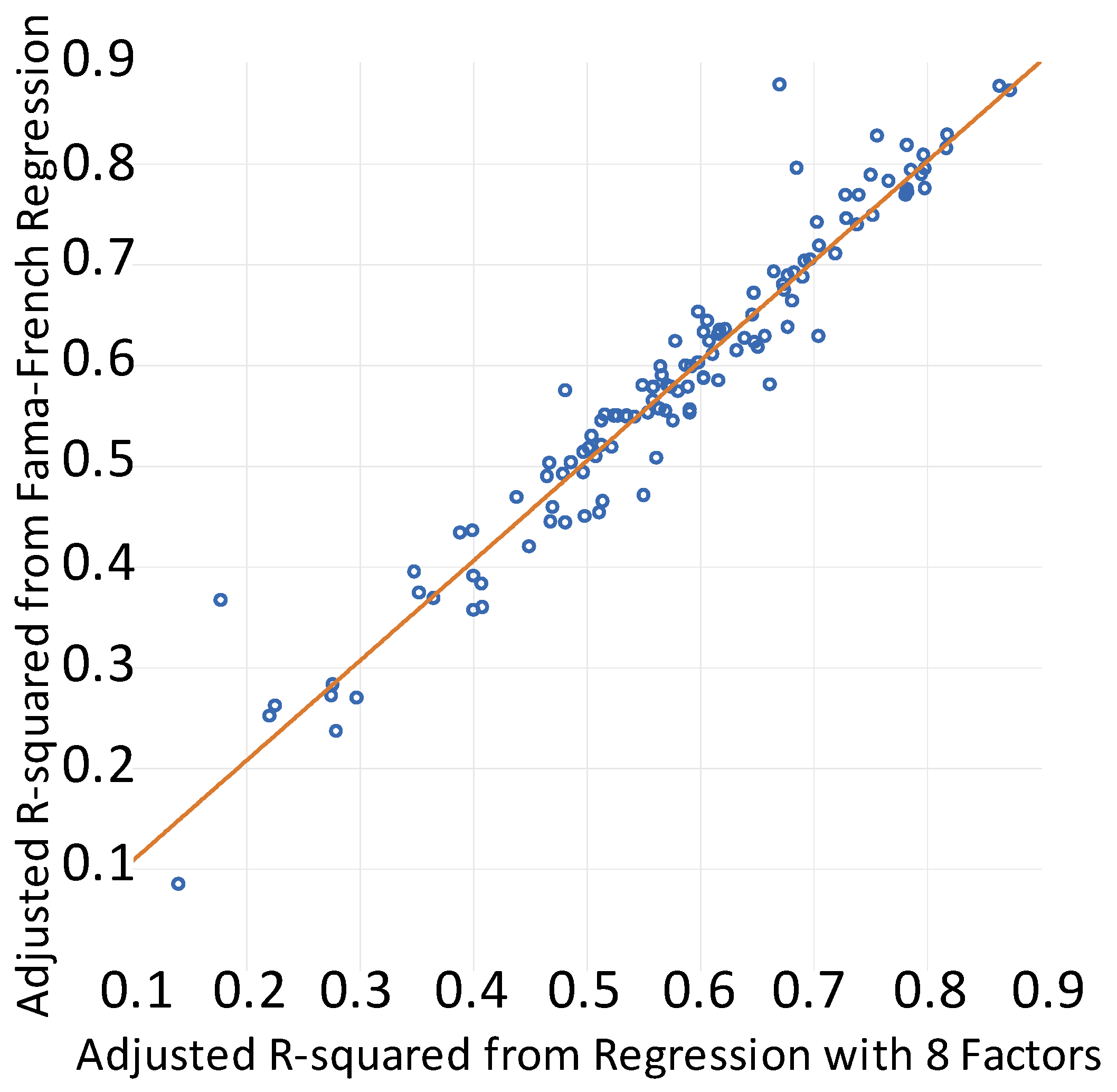
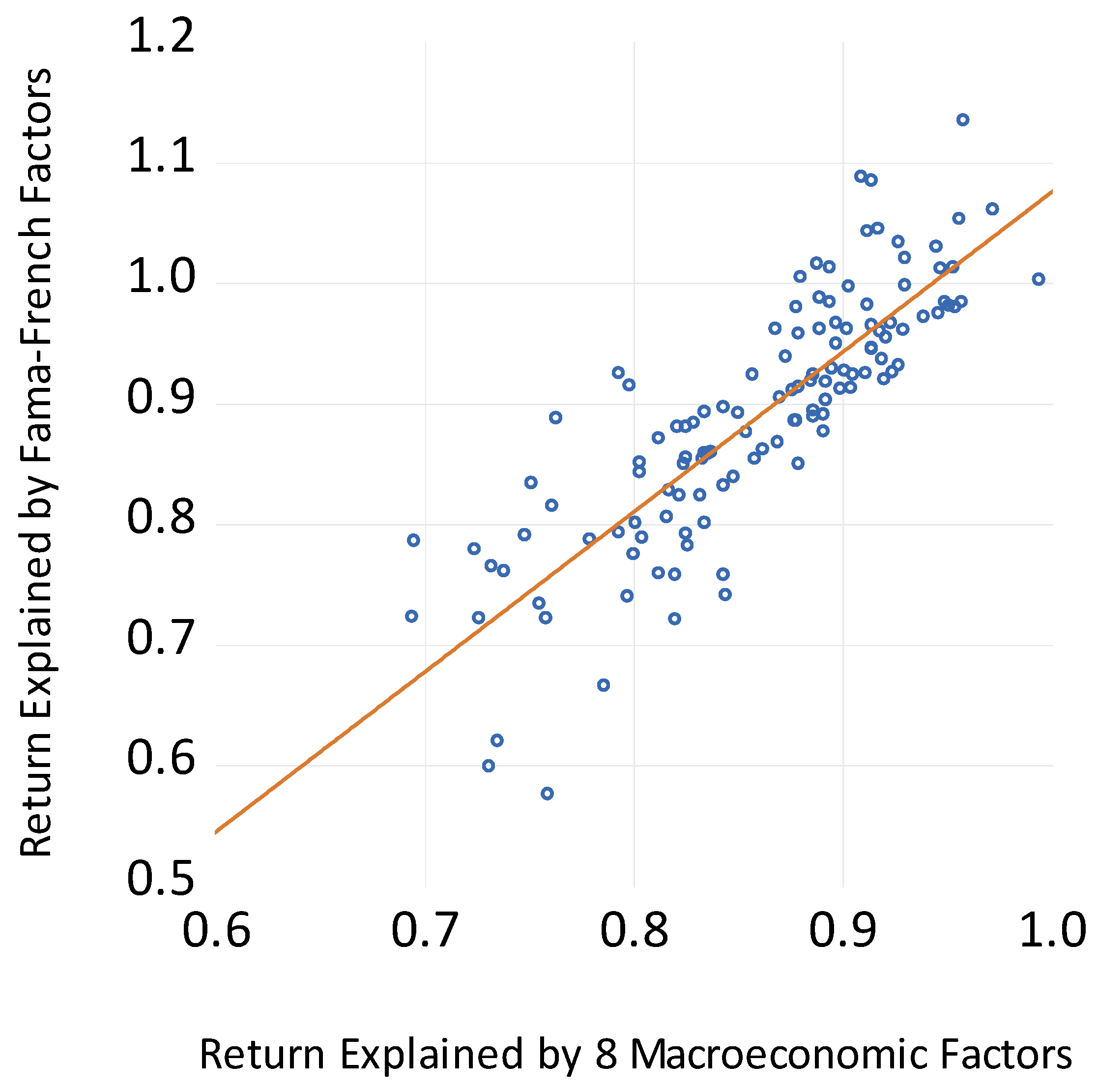
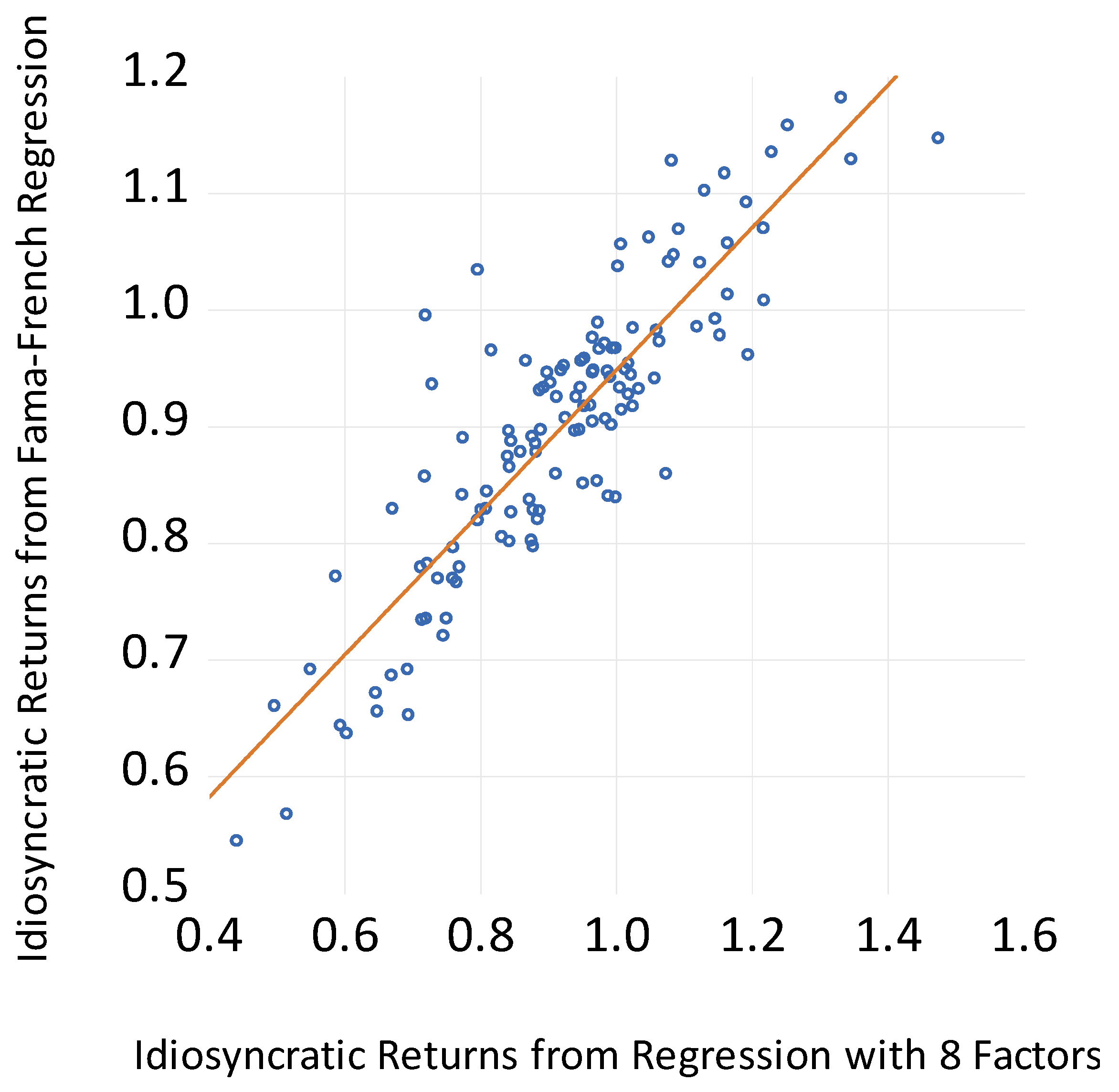
As a robustness test, returns are regressed on the Fama and French (1993, 2015) factors instead of the eight macroeconomic factors. Results for the 125 portfolios are available on request. Interestingly, as Figure 2 shows, the adjusted R-squared figures across sectors for the regressions with the Fama and French factors are closely related to the adjusted R-squared values from the regressions with the eight macroeconomic factors. In addition, as Figure 3 and Figure 4 demonstrate, the influence of systematic and idiosyncratic effects across sectors are similar using these two approaches. The findings in Figure 2, Figure 3 and Figure 4 thus indicate that the results presented in Table 1 are robust to a very different choice of common factors.
The important implication of the findings in this section is that there are large swaths of the U.S. economy whose recovery depends not on the macroeconomic environment but instead on bringing the pandemic under control. These sectors include airlines, aerospace, real estate investment trusts, recreational services, brewers, apparel retailers, and funerals. On the other hand, many sectors that are important for capital investment such as production equipment, machinery, and electronic and electric equipment are dependent on the macroeconomy. A robust recovery is thus necessary to revive business investment.
4. Discussion
The coronavirus pandemic is an exogenous shock. This paper uses sectoral stock price responses to trace out its effects on the U.S. economy. Stock prices are useful because they provide a measure of how investors expect shocks to impact future cash flows across sectors. The paper also decomposes stock return changes into portions driven by sector-specific factors and portions driven by macroeconomic factors. Regressing returns on eight macroeconomic variables and on Fama and French’s (1993, 2015) five factors yield similar decompositions into idiosyncratic and macroeconomic responses.
During the 19 February–10 July 2020 sample period, the coronavirus crisis loomed large as an event driving idiosyncratic responses. Sectors roiled by idiosyncratic factors include airlines, aerospace, real estate, tourism, oil, brewers, retail apparel, and funerals. Until the pandemic is contained, these sectors are likely to suffer. Sectors profiting from idiosyncratic responses include electronic entertainment, diversified retailers such as Amazon, nondurable household goods such as Clorox, biotechnology, computer hardware, and software.
Macroeconomic factors caused large losses in the production equipment, machinery, and electronic and electrical equipment sectors. This suggests that a macroeconomic recovery and not just a defeat of the pandemic is necessary to revive capital goods spending.
News of the crisis contributed to a 43% drop in the aggregate U.S. stock market between 19 February and 23 March 2020. Expansionary policies by the Federal Reserve and the federal government then contributed to a 37% increase in stock prices between 23 March and 10 July 2020. During the recovery period, 7 of the 13 best performing sectors were related to the home and home improvement. This indicates that the stimulus increased peoples’ spending on their homes. While this will make their homes more comfortable, the evidence reported here that the real estate sector has suffered indicates that this spending will not yield a high return on investment.
A stimulus that raises spending in unprofitable areas can falter. Chetty et al. (2020) reported that raising aggregate demand and providing liquidity to businesses may not increase employment much when spending is constrained by health concerns. Policymakers thus need to develop new approaches to promote sustainable recovery from the COVID-19 downturn. One step in this direction, as Barrero et al. (2020) argued, is to avoid subsidizing employee retention in sectors such as airlines where labor demand is unlikely to reach pre-pandemic levels. Instead, incentives should be provided for workers to pursue new jobs in the hope that they find newly productive sectors.
Thorbecke (2020) investigated how the coronavirus crisis has affected sectors of the Japanese stock market. As with the findings for the U.S. economy reported here, idiosyncratic factors during the pandemic caused large losses in sectors related to real estate, travel, and tourism and macroeconomic factors harmed the machinery sector. Future research should investigate how stocks in other countries have been affected and try to explain cross-country differences in responses based on the industrial structures, the level of development, and macroeconomic policy responses.
Funding
This research received no external funding.
Conflicts of Interest
The author declares no conflict of interest.
References
- Aaronson, Daniel, Scott Brave, R. Butters, Daniel Sacks, and Boyoung Seo. 2020. Using the Eye of the Storm to Predict the Wave of COVID-19 UI Claims (No. WP2020-10). Chicago: National Bureau of Economic Research, Available online: https://www.chicagofed.org/research/papers/index (accessed on 24 September 2020).
- Ablan, Jennifer, Philip Georgiadis, Hudson Lockett, and Leo Lewis. 2020. Wall Street rallies for third day as stimulus cheers investors. Financial Times, March 27. [Google Scholar]
- Aït-Sahalia, Yacine, Mustafa Karaman, and Loriano Mancini. 2020. The term structure of equity and variance risk premia. Journal of Econometrics. forthcoming. [Google Scholar]
- Aruoba, S. Boragon, Francis X. Diebold, and Chiara Scotti. 2008. Real time measurement of business conditions. Journal of Business and Economic Statistics 27: 417–27. [Google Scholar] [CrossRef] [Green Version]
- Barrero, Jose Maria, Nicholas Bloom, and Stephen Davis. 2020. COVID-19 Is Also a Reallocation Shock (No. w27137). Cambridge: National Bureau of Economic Research, Available online: https://www.nber.org/papers/w27137 (accessed on 8 August 2020).
- Black, Fischer. 1987. Business Cycles and Equilibrium. New York: Basil Blackwell. [Google Scholar]
- Brower, Derek. 2020. US oil’s slow grind higher. Financial Times, July 28. [Google Scholar]
- Brown, Stephen J., and Jerold B. Warner. 1980. Measuring security price performance. Journal of Financial Economics 8: 205–58. [Google Scholar] [CrossRef]
- Brown, Stephen J., and Jerold B. Warner. 1985. Using daily stock returns: The case of event studies. Journal of Financial Economics 14: 3–31. [Google Scholar] [CrossRef]
- Chan, Kam, and Terry Marsh. 2020. The Asset Markets and the Coronavirus Pandemic. VoxEU Weblog. April 3. Available online: https://voxeu.org/article/asset-markets-and-coronavirus-pandemic (accessed on 20 July 2020).
- Chen, Nai-Fu, Richard Roll, and Stephen A. Ross. 1986. Economic forces and the stock market. The Journal of Business 59: 383–403. [Google Scholar] [CrossRef]
- Chen, Jaikai, Haoyang Liu, David Rubio, Asani Sarkar, and Zhaogang Song. 2020. MBS Market Dysfunction in the Time of COVID-19. Liberty Street Economics Weblog. July 17. Available online: https://libertystreeteconomics.newyorkfed.org/2020/07/mbs-market-dysfunctions-in-the-time-of-covid-19.html (accessed on 26 July 2020).
- Cheng, Jeffrey, Dave Skidmore, and David Wessel. 2020. What’s the Fed Doing in Response to the COVID-19 Crisis? What More Could It Do? Brookings Weblog. July 17. Available online: https://www.brookings.edu/research/fed-response-to-covid19/ (accessed on 25 July 2020).
- Chetty, Raj, John N. Friedman, Nathaniel Hendren, Michael Stepner, and The Opportunity Insights Team. 2020. How Did COVID-19 and Stabilization Policies Affect Spending and Employment? A New Real Time Economic Tracker Based on Private Sector Data. Opportunity Insights Working Paper. Cambridge: Opportunity Insights, Available online: https://opportunityinsights.org/wp-content/uploads/2020/05/tracker_paper.pdf) (accessed on 9 August 2020).
- Dempsey, Harry. 2020. Lumber prices soar to all-time high on renovation demand. Financial Times, August 24. [Google Scholar]
- Dominguez, Kathryn. M. E., and Linda L. Tesar. 2006. Exchange rate exposure. Journal of International Economics 68: 188–218. [Google Scholar] [CrossRef]
- Eichenbaum, Martin, Sergio Rebelo, and Matthias Trabandt. 2020a. Epidemics in the Neoclassical and New Keynesian Models. (No. w27430). Cambridge: National Bureau of Economic Research, Available online: https://www.nber.org/papers/w27430 (accessed on 18 August 2020).
- Eichenbaum, Martin, Sergio Rebelo, and Matthias Trabandt. 2020b. The Macroeconomics of Testing and Quarantining. (No. w27104). Cambridge: National Bureau of Economic Research, Available online: https://www.nber.org/papers/w27104 (accessed on 18 August 2020).
- Eichenbaum, Martin, Sergio Rebelo, and Matthias Trabandt. 2020c. The Macroeconomics of Epidemics (No. w2688 2); Cambridge: National Bureau of Economic Research. Available online: https://www.nber.org/papers/w26882.pdf (accessed on 18 August 2020).
- Fama, Eugene F., and Kenneth R. French. 1993. Common risk factors in the returns on stocks and bonds. Journal of Financial Economics 33: 3–56. [Google Scholar] [CrossRef]
- Fama, Eugene F., and Kenneth R. French. 2015. A five-factor asset pricing model. Journal of Financial Economics 116: 1–22. [Google Scholar] [CrossRef] [Green Version]
- Federal Reserve. 2020. Federal Reserve Announces Extensive New Measures to Support the Economy. March 23. Available online: https://www.federalreserve.gov/newsevents/pressreleases/monetary20200323b.htm (accessed on 25 July 2020).
- Gharib, Chelma, Saima Meyteh-Wali, and Sami Ben Jabeur. 2020. The bubble contagion effect of COVID-19 outbreak: Evidence from crude oil and gold markets. Financial Research Letters. forthcoming. [Google Scholar] [CrossRef] [PubMed]
- Goolsbee, Austan, and Chad Syverson. 2020. Fear, Lockdown, and Diversion: Comparing Drivers of Pandemic Economic Decline 2020 (No w27432). Cambridge: National Bureau of Economic Research, Available online: https://www.nber.org/papers/w27432 (accessed on 25 July 2020).
- Gormsen, Neils Joachim, and Ralph S. J. Koijen. 2020. Coronavirus: Impact on Stock Prices and Growth Expectations (No. w2020-22). Chicago: University of Chicago: Becker Friedman Institute, Available online: https://papers.ssrn.com/sol3/papers.cfm?abstract_id=3555917 (accessed on 17 July 2020).
- Hartley, Jonathan S., and Alessandro Rebucci. 2020. An Event Study of COVID-19 Central Bank Quantitative Easing in Advanced and Emerging Economies (No w27339). Cambridge: National Bureau of Economic Research, Available online: https://www.nber.org/papers/w27339 (accessed on 17 July 2020).
- Koren, Miklos, and Rita Pető. 2020. Business Disruptions from Social Distancing. Covid Economics: Vetted and Real-Time Papers 2. Available online: https://cepr.org/content/covid-economics-vetted-and-real-time-papers-0#block-block-10 (accessed on 18 July 2020).
- Larson, William, and Tara Sinclair. 2020. Nowcasting Unemployment Insurance Claims in the Time of COVID-19 (No. 20-02); Working Paper Series; Washington, DC: Federal Housing Finance Agency. Available online: https://www.fhfa.gov/PolicyProgramsResearch/Research/PaperDocuments/wp2002.pdf (accessed on 25 September 2020).
- Lyocsa, Stefan, Eduard Baumohl, Tomas Vyrost, and Peter Molner. 2020. Fear of the coronavirus and the stock markets. Financial Research Letters 36: 101735. [Google Scholar] [CrossRef] [PubMed]
- McCormick, Myles. 2020. Schlumberger to slash 21,000 jobs as revenues plunge. Financial Times, July 25. [Google Scholar]
- Melek, Nida Cakir. 2018. The response of U.S. investment to oil price shocks: Does the shale boom matter? Economic Review Federal Reserve Bank of Kansas City QIV. , 39–61. Available online: https://www.kc.frb.org/~/media/files/publicat/econrev/econrevarchive/2018/4q18cakirmelek.pdf (accessed on 30 September 2020).
- Noonan, Laura, and Robert Armstrong. 2020. Three US banks set aside record $28bn for loan losses. Financial Times, July 15. [Google Scholar]
- Novet, Jordan. 2020. The PC is Suddenly Cool again … for Now. CNBC. May 4. Available online: https://www.cnbc.com/2020/05/04/pc-sales-usage-rise-during-coronavirus-lockdown.html (accessed on 7 July 2020).
- Pagano, Marco, Christian Wagner, and Josef Zechner. 2020. Disaster Resilience and Asset Prices. Covid Economics: Vetted and Real-Time Papers 2. Available online: https://cepr.org/content/covid-economics-vetted-and-real-time-papers-0#block-block-10 (accessed on 7 August 2020).
- Petralia, Kathryn, Thomas Philippon, Tara Rice, and Nicolas Veron. 2019. Banking Disrupted? Financial Intermediation in an Era of Transformational Technology. Geneva: International Center for Monetary and Banking Studies. [Google Scholar]
- Phillips, Peter C. B., and Shuping Shi. 2018. Financial bubble implosion and reverse regression. Econometric Theory 34: 705–53. [Google Scholar] [CrossRef] [Green Version]
- Promnitz, Donald A. 2020. Broadcasters use free advertising during pandemic. The Business Journal, June 19. [Google Scholar]
- Ramelli, Stefano, and Alexander F. Wagner. 2020. Feverish stock price reactions to COVID-19. Review of Corporate Finance Studies. forthcoming. [Google Scholar] [CrossRef]
- Sharif, Arshan, Aloui Chaker, and Larisa Yarovaya. 2020. Covid-19 pandemic, oil prices, stock market, geopolitical risk and policy uncertainty nexus in the U.S. economy: Fresh evidence from the wavelet based approach. International Review of Financial Analysis 70: 101496. [Google Scholar] [CrossRef]
- Smith, Colby. 2020. US consumers cut debt as lockdowns curbed spending. Financial Times, August 7. [Google Scholar]
- Smith, Colby, and Mamta Badkar. 2020. US stocks post weekly drop as investors reach for safety. Financial Times, February 22. [Google Scholar]
- Thorbecke, Willem. 2019. Oil prices and the U.S. economy: Evidence from the stock market. Journal of Macroeconomics 61: 103137. [Google Scholar] [CrossRef] [Green Version]
- Thorbecke, Willem. 2020. How the Coronavirus Crisis Affected Japanese Industries: Evidence from the Stock Market (No 20-E-061); Tokyo: Research Institute of Economy, Trade and Industry. Available online: www.rieti.go.jp/jp/publications/dp/20e061.pdf (accessed on 17 September 2020).
- Tyco, Kelly. 2020. Need clorox wipes? Disinfecting wipes shortage could last into 2021 amid coronavirus pandemic. USA Today, August 6. [Google Scholar]
- Wells, Peter. 2020. US stocks retreat from record highs. Financial Times, March 27. [Google Scholar]
| 1 | Cheng et al. (2020) provided a valuable discussion of the steps that the Fed has taken. |
| 2 | In some cases, the stock return data are not available until after 4 January 2006. In these cases, the data are employed from the first date they become available. |
| 3 | The business conditions index of Aruoba et al. (2008) was included in exploratory analysis. This variable did not add any explanatory power so it was excluded. |
| 4 | These data come from the Federal Reserve Bank of St. Louis FRED database. |
Figure 1.
U.S. aggregate stock prices. Source: Datastream database.

Figure 2.
Adjusted R-squared coefficients from regressions with eight macroeconomic factors versus adjusted R-squared from regressions with five Fama and French factors. Note: The horizontal axis plots the adjusted R-squared coefficients from regressing daily returns on 125 sectors on the return on the aggregate U.S. stock market index, the return on the world stock market index, the change in the Federal Reserve broad trade-weighted dollar exchange rate index, the change in the log of the spot price for West Texas Intermediate crude oil, the change in the breakeven inflation rate calculated from U.S. Treasury inflation-protected securities, the change in the interest rate on three-month Treasury securities, the change in the spread between interest rates on ten-year and three-month Treasury security, and the change in the spread between interest rates on Moody’s seasoned Baa corporate bonds and ten-year Treasury securities. The vertical axis plots the corresponding adjusted R-squared coefficients from regressing daily returns on 125 sectors on the five Fama and French (2015) factors. These factors are (1) the return on the aggregate U.S. stock market index minus the return on one-month Treasury securities, (2) the average return on nine small capitalization stock portfolios minus the average return on the nine large capitalization stock portfolios, (3) the average return on two high-book value to market value portfolios minus the average return on the two low-book value to market value portfolios, (4) the average return on two robust operating profitability portfolios minus the average return on two weak operating profitability portfolios, and (5) the average return on two conservative investment portfolios minus the average return on two aggressive investment portfolios. Source: Datastream database, Federal Reserve Bank of St. Louis FRED database, homepage of Professor Kenneth French, and calculations by the author.

Figure 3.
Values on 10 July 2020 of One Dollar Invested on 19 February 2020 Explained by Eight Macroeconomic Factors versus Corresponding Values Explained by Fama and French Factors. Note: The horizontal axis measures the values on 10 July 2020 across 125 sectors of a dollar invested on 19 February 2020 explained by 8 macroeconomic factors. These factors are (1) the return on the aggregate U.S. stock market index, (2) the return on the world stock market index, (3) the change in the Federal Reserve broad trade-weighted exchange rate index, (4) the change in the log of the spot price from West Texas Intermediate crude oil, (5) the change in the breakeven inflation rate calculated from U.S. Treasury inflation-protected securities, (6) the change in the interest rate on three-month Treasury securities, (7) the change in the spread between interest rates on ten-year and three-month Treasury security, and (8) the change in the spread between interest rates on Moody’s seasoned Baa corporate bonds and ten-year Treasury securities. The vertical axis plots the corresponding values explained by the five Fama and French (2015) factors. These factors are (1) the return on the aggregate U.S. stock market index minus the return on one-month Treasury securities, (2) the average return on nine small capitalization stock portfolios minus the average return on the nine large capitalization stock portfolios, (3) the average return on two high-book value to market value portfolios minus the average return on the two low-book value to market value portfolios, (4) the average return on two robust operating profitability portfolios minus the average return on two weak operating profitability portfolios, and (5) the average return on two conservative investment portfolios minus the average return on two aggressive investment portfolios. Source: Datastream database, Federal Reserve Bank of St. Louis FRED database, homepage of Professor Kenneth French, and calculations by the author.

Figure 4.
Values on 10 July 2020 of one dollar invested on 19 February 2020 not explained by eight macroeconomic factors versus corresponding values not explained by Fama and French factors. Note: The horizontal axis measures the values on 10 July 2020 across 125 sectors of a dollar invested on 19 February 2020 not explained by 8 macroeconomic factors. These factors are (1) the return on the aggregate U.S. stock market index, (2) the return on the world stock market index, (3) the change in the Federal Reserve broad trade-weighted exchange rate index, (4) the change in the log of the spot price from West Texas Intermediate crude oil, (5) the change in the breakeven inflation rate calculated from U.S. Treasury inflation-protected securities, (6) the change in the interest rate on three-month Treasury securities, (7) the change in the spread between interest rates on ten-year and three-month Treasury security, and (8) the change in the spread between interest rates on Moody’s seasoned Baa corporate bonds and ten-year Treasury securities. The vertical axis plots the corresponding values not explained by the five Fama and French (2015) factors. These factors are (1) the return on the aggregate U.S. stock market index minus the return on one-month Treasury securities, (2) the average return on nine small capitalization stock portfolios minus the average return on the nine large capitalization stock portfolios, (3) the average return on two high-book value to market value portfolios minus the average return on the two low-book value to market value portfolios, (4) the average return on two robust operating profitability portfolios minus the average return on two weak operating profitability portfolios, and (5) the average return on two conservative investment portfolios minus the average return on two aggressive investment portfolios. Changes in value not explained by macroeconomic factors over the 19 February–10 July 2020 period include sector-specific responses to the COVID-19 pandemic. Source: Datastream database, Federal Reserve Bank of St. Louis FRED database, homepage of Professor Kenneth French, and calculations by the author.


Table 1.
Value of one dollar invested across U.S. sectors explained by eight macroeconomic variables and by sector-specific factors.
Table 1.
Value of one dollar invested across U.S. sectors explained by eight macroeconomic variables and by sector-specific factors.
| Value on 10 July 2020 of One Dollar Invested on 19 February 2020 | Value on 23 March 2020 of One Dollar Invested on 19 February 2020 | Value on 10 July 2020 of One Dollar Invested on 23 March 2020 | |||||||
|---|---|---|---|---|---|---|---|---|---|
| (1) | (2) | (3) | (4) | (5) | (6) | (7) | (8) | (9) | (10) |
| Sector | Due to all factors | Due to macro factors | Due to sector-specific factors | Due to all factors | Due to macro factors | Due to sector-specific factors | Due to all factors | Due to macro factors | Due to sector-specific factors |
| Aerospace | 0.500 | 0.834 | 0.604 | 0.377 | 0.546 | 0.703 | 1.32 | 1.472 | 0.885 |
| Airlines | 0.381 | 0.812 | 0.442 | 0.381 | 0.539 | 0.704 | 1.039 | 1.452 | 0.676 |
| Apparel Retailer | 0.652 | 0.862 | 0.766 | 0.492 | 0.592 | 0.833 | 1.284 | 1.419 | 0.913 |
| Automobiles | 1.225 | 0.801 | 1.253 | 0.468 | 0.524 | 0.882 | 2.601 | 1.468 | 1.469 |
| Banks | 0.577 | 0.759 | 0.72 | 0.489 | 0.509 | 0.942 | 1.078 | 1.426 | 0.732 |
| Basic Materials | 0.897 | 0.812 | 1.06 | 0.595 | 0.538 | 1.088 | 1.43 | 1.444 | 0.967 |
| Basic Resources | 0.925 | 0.751 | 1.124 | 0.609 | 0.483 | 1.211 | 1.456 | 1.475 | 0.936 |
| Beverages | 0.816 | 0.951 | 0.888 | 0.649 | 0.749 | 0.875 | 1.236 | 1.246 | 1.015 |
| Biotechnology | 1.125 | 0.958 | 1.195 | 0.795 | 0.728 | 1.092 | 1.396 | 1.292 | 1.101 |
| Brewers | 0.587 | 0.899 | 0.695 | 0.615 | 0.708 | 0.874 | 0.891 | 1.24 | 0.761 |
| Cable TV Services | 0.876 | 0.892 | 0.947 | 0.682 | 0.624 | 1.083 | 1.308 | 1.388 | 0.916 |
| Casinos/Gambling | 0.554 | 0.738 | 0.715 | 0.472 | 0.471 | 0.989 | 1.201 | 1.486 | 0.777 |
| Chemicals | 0.881 | 0.85 | 1.019 | 0.589 | 0.576 | 1.015 | 1.415 | 1.418 | 0.988 |
| Clothing, Accessories | 0.747 | 0.858 | 0.846 | 0.531 | 0.592 | 0.894 | 1.342 | 1.399 | 0.935 |
| Commercial Vehicle Leasing | 0.575 | 0.726 | 0.774 | 0.331 | 0.421 | 0.777 | 1.668 | 1.623 | 1.017 |
| Computer Hardware | 1.099 | 0.912 | 1.165 | 0.668 | 0.637 | 1.054 | 1.614 | 1.391 | 1.115 |
| Computer Services | 0.884 | 0.894 | 0.994 | 0.641 | 0.661 | 0.973 | 1.366 | 1.316 | 1.039 |
| Consumer Digital Services | 1.009 | 0.914 | 1.074 | 0.664 | 0.664 | 0.996 | 1.503 | 1.341 | 1.095 |
| Construction and Materials | 0.805 | 0.836 | 0.913 | 0.59 | 0.561 | 1.029 | 1.307 | 1.433 | 0.884 |
| Construction | 0.617 | 0.761 | 0.761 | 0.553 | 0.489 | 1.095 | 1.149 | 1.48 | 0.75 |
| Consumer Electronics | 0.946 | 0.879 | 1.026 | 0.637 | 0.632 | 0.998 | 1.43 | 1.347 | 1.023 |
| Consumer Lending | 0.58 | 0.8 | 0.713 | 0.426 | 0.507 | 0.826 | 1.296 | 1.515 | 0.854 |
| Consumer Staples | 0.88 | 0.946 | 0.94 | 0.706 | 0.749 | 0.949 | 1.202 | 1.239 | 0.974 |
| Consumer Services | 0.945 | 0.903 | 1.009 | 0.589 | 0.651 | 0.902 | 1.601 | 1.351 | 1.145 |
| Containers and Packaging | 0.87 | 0.886 | 0.954 | 0.635 | 0.637 | 0.992 | 1.266 | 1.347 | 0.918 |
| Copper | 0.969 | 0.695 | 1.193 | 0.524 | 0.41 | 1.226 | 1.738 | 1.584 | 0.977 |
| Cosmetics | 0.757 | 0.927 | 0.797 | 0.621 | 0.664 | 0.942 | 1.188 | 1.355 | 0.849 |
| Defense | 0.707 | 0.914 | 0.77 | 0.597 | 0.679 | 0.885 | 1.119 | 1.314 | 0.843 |
| Delivery Service | 0.998 | 0.891 | 1.078 | 0.78 | 0.672 | 1.153 | 1.27 | 1.289 | 0.956 |
| Distillers and Vintners | 0.852 | 0.912 | 0.989 | 0.561 | 0.665 | 0.846 | 1.38 | 1.335 | 1.092 |
| Diversified Retailers | 1.296 | 0.972 | 1.218 | 0.873 | 0.758 | 1.148 | 1.511 | 1.261 | 1.098 |
| Drug Retailers | 0.816 | 0.918 | 0.877 | 0.748 | 0.72 | 1.044 | 1.039 | 1.246 | 0.819 |
| Education Services | 0.669 | 0.889 | 0.751 | 0.522 | 0.631 | 0.841 | 1.301 | 1.379 | 0.926 |
| Electronic and Electrical Equipment | 0.843 | 0.857 | 0.954 | 0.606 | 0.588 | 1.023 | 1.319 | 1.403 | 0.92 |
| Electronic Entertainment | 1.365 | 0.909 | 1.475 | 0.851 | 0.657 | 1.279 | 1.692 | 1.35 | 1.244 |
| Electronic Equipment: Controls | 0.846 | 0.829 | 0.968 | 0.582 | 0.552 | 1.038 | 1.37 | 1.44 | 0.918 |
| Electronic Equipment: Gauges | 0.868 | 0.889 | 0.963 | 0.638 | 0.627 | 1.014 | 1.306 | 1.369 | 0.944 |
| Electronic Equipment: Pollution Control | 0.733 | 0.869 | 0.802 | 0.581 | 0.606 | 0.955 | 1.196 | 1.381 | 0.827 |
| Electricity | 0.757 | 0.914 | 0.879 | 0.607 | 0.695 | 0.882 | 1.178 | 1.289 | 0.96 |
| Electronic Components | 0.822 | 0.834 | 0.942 | 0.595 | 0.562 | 1.046 | 1.35 | 1.425 | 0.916 |
| Entertainment | 0.98 | 0.886 | 1.034 | 0.694 | 0.626 | 1.101 | 1.461 | 1.374 | 1 |
| Farming and Fishing | 0.741 | 0.895 | 0.832 | 0.668 | 0.67 | 1.007 | 1.091 | 1.295 | 0.838 |
| Fertilizers | 0.754 | 0.763 | 1 | 0.535 | 0.477 | 1 | 1.351 | 1.515 | 1 |
| Financial Data Providers | 0.986 | 0.873 | 1.147 | 0.601 | 0.58 | 1.031 | 1.526 | 1.454 | 1.07 |
| Food Products | 0.927 | 0.939 | 0.988 | 0.728 | 0.748 | 0.976 | 1.21 | 1.233 | 0.981 |
| Footwear | 0.89 | 0.929 | 0.948 | 0.592 | 0.675 | 0.874 | 1.406 | 1.339 | 1.045 |
| Forestry | 0.627 | 0.885 | 0.721 | 0.453 | 0.643 | 0.726 | 1.125 | 1.34 | 0.832 |
| Fruit and Grain | 0.799 | 0.843 | 0.926 | 0.635 | 0.605 | 1.046 | 1.233 | 1.344 | 0.899 |
| Funerals | 0.684 | 0.905 | 0.76 | 0.679 | 0.633 | 1.066 | 1.002 | 1.383 | 0.732 |
| Gas Distribution | 0.719 | 0.879 | 0.844 | 0.592 | 0.635 | 0.942 | 1.153 | 1.345 | 0.876 |
| General Industrials | 0.788 | 0.848 | 0.899 | 0.58 | 0.604 | 0.953 | 1.259 | 1.357 | 0.905 |
| Gold Mining | 1.241 | 0.927 | 1.332 | 0.854 | 0.707 | 1.186 | 1.5 | 1.281 | 1.184 |
| Health Care | 0.955 | 0.945 | 1.019 | 0.703 | 0.721 | 0.978 | 1.293 | 1.284 | 1.013 |
| Household Appliance | 0.782 | 0.834 | 0.924 | 0.402 | 0.562 | 0.721 | 1.66 | 1.428 | 1.14 |
| Household Equipment Producers | 0.689 | 0.826 | 0.843 | 0.496 | 0.6 | 0.824 | 1.279 | 1.322 | 0.982 |
| Household Furnishing | 0.895 | 0.822 | 1.082 | 0.421 | 0.533 | 0.79 | 2.164 | 1.487 | 1.444 |
| Home Construction | 0.743 | 0.82 | 0.904 | 0.414 | 0.531 | 0.766 | 1.625 | 1.49 | 1.11 |
| Home Improvement Retail | 0.953 | 0.892 | 1.093 | 0.592 | 0.624 | 0.966 | 1.698 | 1.391 | 1.223 |
| Hotel and Lodging REIT | 0.393 | 0.731 | 0.498 | 0.386 | 0.456 | 0.821 | 1.029 | 1.53 | 0.64 |
| Hotels and Motels | 0.581 | 0.816 | 0.67 | 0.477 | 0.539 | 0.848 | 1.178 | 1.449 | 0.797 |
| Industrial Engineering | 0.843 | 0.824 | 1 | 0.592 | 0.542 | 1 | 1.359 | 1.454 | 1 |
| Industrial Materials | 0.659 | 0.798 | 0.775 | 0.497 | 0.519 | 0.952 | 1.146 | 1.471 | 0.738 |
| Industrial Suppliers | 0.832 | 0.886 | 0.92 | 0.547 | 0.622 | 0.888 | 1.407 | 1.38 | 0.992 |
| Industrial Support Services | 0.854 | 0.902 | 0.966 | 0.584 | 0.639 | 0.921 | 1.398 | 1.371 | 1.033 |
| Industrial Transport | 0.879 | 0.878 | 0.966 | 0.633 | 0.618 | 1.02 | 1.355 | 1.376 | 0.954 |
| Investment Services | 0.811 | 0.755 | 1.003 | 0.567 | 0.5 | 1.104 | 1.324 | 1.443 | 0.882 |
| Iron and Steel | 0.771 | 0.724 | 0.966 | 0.58 | 0.455 | 1.216 | 1.249 | 1.505 | 0.789 |
| Leisure Goods | 1.231 | 0.894 | 1.347 | 0.764 | 0.65 | 1.164 | 1.677 | 1.338 | 1.236 |
| Life Insurance | 0.583 | 0.735 | 0.73 | 0.415 | 0.455 | 0.897 | 1.355 | 1.538 | 0.824 |
| Luxury Items | 0.881 | 0.911 | 0.883 | 0.893 | 0.667 | 1.28 | 0.957 | 1.327 | 0.689 |
| Machinery: Agricultural | 0.852 | 0.837 | 0.976 | 0.633 | 0.548 | 1.136 | 1.329 | 1.458 | 0.887 |
| Machinery: Construction | 0.868 | 0.825 | 1.064 | 0.65 | 0.55 | 1.151 | 1.284 | 1.435 | 0.929 |
| Machinery: Engines | 0.973 | 0.803 | 1.049 | 0.601 | 0.505 | 1.118 | 1.417 | 1.514 | 0.865 |
| Machinery: Industrial | 0.72 | 0.833 | 0.844 | 0.471 | 0.55 | 0.852 | 1.463 | 1.454 | 0.987 |
| Machinery: Specialty | 0.803 | 0.876 | 0.912 | 0.675 | 0.616 | 1.083 | 1.139 | 1.371 | 0.836 |
| Machinery: Tools | 0.756 | 0.843 | 0.894 | 0.477 | 0.556 | 0.855 | 1.458 | 1.459 | 1.001 |
| Media Agencies | 0.824 | 0.825 | 0.985 | 0.549 | 0.583 | 0.943 | 1.476 | 1.367 | 1.063 |
| Medical Equipment | 0.947 | 0.93 | 1.025 | 0.66 | 0.68 | 0.969 | 1.361 | 1.332 | 1.03 |
| Medical Services | 0.84 | 0.93 | 0.952 | 0.529 | 0.693 | 0.778 | 1.51 | 1.314 | 1.191 |
| Medical Supplies | 0.912 | 0.956 | 0.973 | 0.666 | 0.722 | 0.924 | 1.287 | 1.298 | 1.011 |
| Metal Fabric. | 0.99 | 0.901 | 1.086 | 0.663 | 0.628 | 1.045 | 1.46 | 1.388 | 1.05 |
| Mortgage REITs | 0.478 | 0.844 | 0.551 | 0.387 | 0.588 | 0.669 | 1.111 | 1.398 | 0.762 |
| Nondurable Household Products | 1.213 | 0.994 | 1.23 | 0.903 | 0.831 | 1.086 | 1.267 | 1.18 | 1.085 |
| Nonlife Insurance | 0.746 | 0.879 | 0.841 | 0.628 | 0.65 | 0.967 | 1.127 | 1.317 | 0.848 |
| Office REITs | 0.62 | 0.82 | 0.719 | 0.525 | 0.533 | 0.966 | 1.135 | 1.478 | 0.743 |
| Oil Equipment and Services | 0.418 | 0.694 | 0.595 | 0.311 | 0.431 | 0.749 | 1.259 | 1.523 | 0.788 |
| Oil Refining and Marketing | 0.55 | 0.748 | 0.723 | 0.361 | 0.467 | 0.773 | 1.294 | 1.529 | 0.837 |
| Oil: Crude Prod. | 0.45 | 0.732 | 0.647 | 0.31 | 0.461 | 0.709 | 1.381 | 1.514 | 0.912 |
| Oil and Gas (International) | 0.656 | 0.817 | 0.797 | 0.477 | 0.567 | 0.851 | 1.288 | 1.393 | 0.909 |
| Paint and Coating | 0.891 | 0.924 | 0.949 | 0.615 | 0.654 | 0.938 | 1.364 | 1.375 | 0.98 |
| Paper | 0.721 | 0.797 | 0.817 | 0.578 | 0.53 | 1.077 | 1.112 | 1.438 | 0.71 |
| Personal Goods | 0.825 | 0.919 | 0.89 | 0.593 | 0.688 | 0.867 | 1.324 | 1.303 | 1.001 |
| Personal Product | 0.949 | 0.957 | 0.992 | 0.759 | 0.767 | 0.997 | 1.195 | 1.226 | 0.969 |
| Pharmaceuticals | 0.961 | 0.953 | 1.014 | 0.75 | 0.751 | 0.999 | 1.215 | 1.245 | 0.981 |
| Pipelines | 0.55 | 0.821 | 0.694 | 0.398 | 0.591 | 0.701 | 1.258 | 1.347 | 0.932 |
| Production Technology and Equipment | 0.932 | 0.878 | 1.023 | 0.598 | 0.582 | 1.034 | 1.61 | 1.456 | 1.057 |
| Professional Business Support | 0.889 | 0.897 | 1.006 | 0.617 | 0.643 | 0.962 | 1.391 | 1.354 | 1.041 |
| Publishing | 0.918 | 0.87 | 0.974 | 0.64 | 0.643 | 0.99 | 1.381 | 1.315 | 0.976 |
| Radio TV Broadcasting | 0.657 | 0.779 | 0.81 | 0.47 | 0.503 | 0.916 | 1.387 | 1.482 | 0.916 |
| Railroad Equipment | 0.64 | 0.832 | 0.738 | 0.486 | 0.546 | 0.872 | 1.33 | 1.462 | 0.888 |
| Railroads | 0.806 | 0.877 | 0.888 | 0.576 | 0.59 | 0.978 | 1.342 | 1.439 | 0.902 |
| Real Estate Holdings and Development | 0.413 | 0.758 | 0.516 | 0.319 | 0.468 | 0.686 | 1.115 | 1.539 | 0.683 |
| Real Estate | 0.742 | 0.843 | 0.868 | 0.556 | 0.567 | 0.967 | 1.26 | 1.438 | 0.877 |
| Recreation Products | 1.013 | 0.891 | 1.131 | 0.578 | 0.584 | 0.977 | 1.758 | 1.472 | 1.202 |
| Recreational Vehicles | 0.829 | 0.825 | 1.008 | 0.402 | 0.515 | 0.795 | 1.755 | 1.534 | 1.132 |
| Recreational Services | 0.507 | 0.793 | 0.649 | 0.41 | 0.53 | 0.784 | 1.265 | 1.437 | 0.88 |
| Renewable Energy Equipment | 1.102 | 0.793 | 1.219 | 0.585 | 0.496 | 1.129 | 1.864 | 1.525 | 1.12 |
| Restaurants and Bars | 0.82 | 0.949 | 0.873 | 0.606 | 0.709 | 0.863 | 1.305 | 1.313 | 0.996 |
| Retail REITs | 0.469 | 0.786 | 0.588 | 0.399 | 0.506 | 0.796 | 1.109 | 1.492 | 0.727 |
| Retailers | 1.184 | 0.947 | 1.165 | 0.786 | 0.718 | 1.092 | 1.536 | 1.292 | 1.109 |
| Security Services | 0.753 | 0.854 | 0.86 | 0.53 | 0.594 | 0.887 | 1.338 | 1.393 | 0.945 |
| Semiconductors | 0.963 | 0.88 | 1.058 | 0.67 | 0.605 | 1.113 | 1.494 | 1.406 | 1.019 |
| Soft Drinks | 0.814 | 0.954 | 0.879 | 0.66 | 0.756 | 0.882 | 1.223 | 1.24 | 1.005 |
| Software | 1.065 | 0.917 | 1.154 | 0.698 | 0.648 | 1.082 | 1.519 | 1.377 | 1.091 |
| Specialty Retail | 0.906 | 0.897 | 0.995 | 0.564 | 0.631 | 0.897 | 1.617 | 1.385 | 1.145 |
| Technology Hardware | 1.029 | 0.888 | 1.12 | 0.663 | 0.617 | 1.081 | 1.562 | 1.395 | 1.075 |
| Telecommunications | 0.901 | 0.904 | 0.984 | 0.732 | 0.698 | 1.05 | 1.213 | 1.266 | 0.945 |
| Tobacco | 0.81 | 0.923 | 0.885 | 0.666 | 0.726 | 0.929 | 1.162 | 1.247 | 0.928 |
| Toys | 0.691 | 0.868 | 0.746 | 0.508 | 0.612 | 0.833 | 1.466 | 1.379 | 0.99 |
| Training, Employment | 0.746 | 0.803 | 0.882 | 0.521 | 0.538 | 0.939 | 1.382 | 1.434 | 0.943 |
| Transport Services | 0.655 | 0.804 | 0.809 | 0.404 | 0.51 | 0.799 | 1.761 | 1.514 | 1.14 |
| Travel and Tourism | 0.567 | 0.804 | 0.672 | 0.407 | 0.512 | 0.792 | 1.404 | 1.503 | 0.892 |
| Trucking | 1.103 | 0.92 | 1.161 | 0.761 | 0.674 | 1.114 | 1.434 | 1.329 | 1.059 |
| Utilities | 0.759 | 0.914 | 0.876 | 0.611 | 0.692 | 0.892 | 1.168 | 1.294 | 0.944 |
| Waste and Disposal Services | 0.77 | 0.921 | 0.846 | 0.646 | 0.696 | 0.934 | 1.075 | 1.291 | 0.84 |
Note: Column (2) presents the stock market return as of 10 July 2020 from investing 1 dollar in the sector listed in column (1) on 19 February 2020. Column (3) presents the portion of returns in column (2) that can be attributed to the effect of eight macroeconomic factors on returns. These factors are (1) the return on the aggregate U.S. stock market index, (2) the return on the world stock market index, (3) the change in the Federal Reserve broad trade-weighted exchange rate index, (4) the change in the log of the spot price from West Texas Intermediate crude oil, (5) the change in the breakeven inflation rate calculated from U.S. Treasury inflation-protected securities, (6) the change in the interest rate on three-month Treasury securities, (7) the change in the spread between interest rates on ten-year and three-month Treasury security, and (8) the change in the spread between interest rates on Moody’s seasoned Baa corporate bonds and ten-year Treasury securities. Column (4) presents the portion of returns in column (2) not explained by these eight factors. Column (4) thus includes the effects of other factors such as the coronavirus pandemic on returns. Column (5)–(7) and (8)–(10) are analogous to columns (2)–(4) except the returns on a one-dollar investment are calculated over the 19 February 2020–23 March 2020 and 23 March 2020–10 July 2020 periods, respectively. Column (11) presents the adjusted R-squared coefficient from a regression of the sector’s return on the eight macroeconomic factors. The sample period extends from 4 January 2006 to 10 July 2020. In cases where return data are not available on 4 January 2006, the sample begins on the first date when return data become available. Source: Datastream database, Federal Reserve Bank of St. Louis FRED database, and calculations by the author.
Table 2.
The exposures of industry portfolios to macroeconomic variables.
| (1) | (2) | (3) | (4) | (5) | (6) | (7) | (8) | (9) | (10) |
|---|---|---|---|---|---|---|---|---|---|
| Sector | U.S. Stock Market Beta | World Stock Market Beta | Exchange Rate Beta | Oil Price Beta | Inflation Beta | Three-Month Treasury Rate Beta | Ten-Year Treasury Rate Minus Three-Month Treasury Rate Beta | Baa Corporate Bond Rate Minus Ten-Year Treasury Rate Beta | Adjusted-R2 |
| Aerospace | 0.978 *** (0.041) | 0.156 *** (0.056) | −0.003 (0.008) | 0.025 *** (0.0125) | 0.079 (0.057) | −0.125 (0.102) | −0.065 (0.100) | −0.380 ** (0.160) | 0.674 |
| Airlines | 1.278 *** (0.089) | −0.061 (0.117) | 0.008 (0.024) | 0.014 (0.025) | −0.159 (0.146) | −0.161 (0.189) | −0.128 (0.164) | −0.390 (0.330) | 0.349 |
| Apparel Retailer | 1.175 *** (0.037) | −0.152 *** (0.056) | 0.009 (0.009) | 0.037 ** (0.016) | −0.016 (0.048) | 0.039 (0.084) | 0.022 (0.054) | −0.143 (0.088) | 0.607 |
| Automobiles | 1.148 *** (0.085) | 0.309 *** (0.100) | 0.022 (0.015) | −0.077 *** (0.010) | 0.059 (0.075) | −0.011 (0.131) | 0.038 (0.115) | 0.047 (0.195) | 0.487 |
| Banks | 1.632 *** (0.086) | −0.204 *** (0.074) | 0.010 (0.014) | −0.010 (0.011) | −0.090 (0.078) | 0.373 ** (0.160) | 0.333 *** (0.094) | 0.120 (0.178) | 0.671 |
| Basic Materials | 1.032 *** (0.049) | 0.215 *** (0.060) | −0.042 *** (0.008) | 0.042 *** (0.010) | 0.073 (0.063) | 0.110* (0.060) | 0.118 *** (0.037) | 0.052 (0.078) | 0.782 |
| Basic Resources | 1.110 *** (0.085) | 0.262 *** (0.095) | −0.078 *** (0.012) | 0.047 * (0.020) | 0.099 (0.128) | 0.100 (0.087) | 0.039 (0.056) | 0.084 (0.121) | 0.649 |
| Beverages | 0.648 *** (0.034) | −0.033 (0.044) | −0.075 (0.067) | 0.014 (0.010) | −0.054 (0.037) | −0.013 *** (0.045) | −0.097 *** (0.035) | −0.140 (0.094) | 0.567 |
| Biotechnology | 0.849 *** (0.048) | −0.057 (0.055) | 0.016 ** (0.008) | −0.068 *** (0.009) | 0.010 (0.046) | −0.095* (0.056) | −0.021 (0.046) | 0.011 (0.085) | 0.482 |
| Brewers | 0.583 *** (0.054) | 0.085 (0.064) | −0.022 * (0.011) | 0.000 (0.000) | −0.028 (0.049) | −0.063 (0.068) | −0.046 (0.052) | −0.156 (0.131) | 0.277 |
| Cable TV Services | 1.109 *** (0.053) | −0.113 * (0.065) | −0.029 (0.097) | −0.016 *** (0.004) | −0.025 (0.627) | 0.044 (0.065) | −0.030 (0.052) | −0.054 (0.124) | 0.590 |
| Casinos/Gambling | 1.121 *** (0.125) | 0.506 *** (0.140) | −0.217 (0.180) | 0.086 *** (0.017) | 0.569 (0.904) | 0.059 (0.105) | 0.074 (0.105) | 0.199 (0.199) | 0.505 |
| Chemicals | 0.992 *** (0.035) | 0.156 *** (0.047) | −0.255 *** (0.065) | 0.038 *** (0.005) | 0.545 (0.332) | 0.105 ** (0.053) | 0.153 *** (0.034) | 0.029 (0.069) | 0.784 |
| Clothing, Accessories | 1.121 *** (0.041) | 0.090 (0.063) | 0.176 * (0.099) | 0.011 (0.012) | 0.907 ** (0.434) | −0.047 (0.779) | 0.115 ** (0.052) | 0.080 (0.112) | 0.618 |
| Commercial Vehicle Leasing | 1.054 *** (0.101) | 0.632 *** (0.151) | −0.308 (0.239) | 0.111 *** (0.013) | −0.122 (0.244) | −0.053 (0.173) | 0.029 (0.154) | −0.318 (0.112) | 0.498 |
| Computer Hardware | 1.003 *** (0.037) | 0.007 (0.050) | 0.117 (0.075) | 0.005 (0.004) | 0.018 (0.077) | 0.382 (0.597) | 0.042 (0.051) | −0.034 (0.066) | 0.579 |
| Computer Services | 1.850 *** (0.037) | 0.044 (0.038) | −0.023 (0.059) | −0.043 *** (0.003) | −0.004 (0.047) | 0.542 (0.438) | 0.036 (0.032) | −0.030 (0.048) | 0.691 |
| Consumer Digital Services | 0.987 *** (0.044) | 0.033 (0.064) | 0.215 ** (0.089) | −0.033 *** (0.003) | −0.220 (0.040) | −0.485 (0.875) | −0.029 (0.516) | 0.085 (0.109) | 0.517 |
| Construction and Materials | 1.063 *** (0.038) | 0.215 *** (0.049) | −0.071 (0.089) | 0.042 *** (0.006) | 0.882 ** (0.431) | 0.123 (0.508) | 0.060 (0.040) | 0.102 (0.088) | 0.799 |
| Construction | 1.110 *** (0.059) | 0.406 *** (0.096) | −0.273 (0.167) | 0.112 *** (0.019) | 0.245 ** (0.117) | 0.123 (0.997) | 0.168 ** (0.075) | 0.262 * (0.145) | 0.640 |
| Consumer Electronics | 0.973 *** (0.073) | −0.018 (0.102) | −0.164 (0.134) | 0.024 *** (0.005) | −0.674 (0.649) | 0.218 (0.152) | 0.093 (0.075) | −0.092 (0.127) | 0.276 |
| Consumer Lending | 1.412 *** (0.054) | −0.159 ** (0.068) | −0.038 (0.128) | −0.050 ** (0.017) | −0.444 (0.524) | 0.406 (0.858) | −0.004 (0.076) | −0.363 (0.146) | 0.705 |
| Consumer Staples | 0.691 *** (0.024) | −0.037 (0.033) | −0.052 (0.052) | 0.008 (0.006) | −0.513 (0.388) | −0.098 (0.038) | −0.077 (0.031) | −0.049 (0.058) | 0.741 |
| Consumer Services | 0.983 *** (0.033) | −0.017 (0.051) | 0.124 * (0.075) | −0.023 *** (0.005) | −0.022 (0.470) | −0.130 * (0.069) | −0.017 (0.065) | −0.104 (0.089) | 0.612 |
| Containers and Packaging | 0.938 *** (0.029) | 0.092 ** (0.039) | −0.029 (0.061) | 0.013 *** (0.005) | −0.134 (0.340) | −0.077 (0.575) | 0.012 (0.041) | 0.061 (0.064) | 0.739 |
| Copper | 1.129 *** (0.102) | 0.444 *** (0.137) | −0.128 *** (0.191) | 0.055 ** (0.022) | 0.192 (0.119) | 0.240 ** (0.113) | 0.193 ** (0.075) | 0.114 (0.161) | 0.551 |
| Cosmetics | 0.855 *** (0.058) | 0.109 (0.076) | −0.211 ** (0.101) | 0.248 ** (0.109) | −0.293 (0.485) | −0.110 (0.116) | −0.045 (0.548) | 0.073 (0.105) | 0.401 |
| Defense | 0.760 *** (0.038) | 0.056 (0.048) | 0.109 (0.880) | 0.033 *** (0.012) | 0.140 (0.422) | −0.149 (0.575) | 0.007 (0.042) | −0.165 ** (0.0765) | 0.581 |
| Delivery Service | 0.928 *** (0.039) | 0.024 (0.051) | 0.025 (0.085) | 0.031 *** (0.010) | −0.650 (0.570) | 0.355 (0.786) | 0.118 * (0.061) | 0.092 (0.138) | 0.609 |
| Distillers and Vintners | 0.684 *** (0.044) | 0.132 ** (0.064) | −0.047 (0.090) | 0.056 *** (0.011) | −0.373 (0.763) | −0.123 * (0.079) | −0.0788 (0.0048) | −0.271 (0.103) | 0.469 |
| Diversified Retailers | 0.885 *** (0.038) | −0.016 *** (0.047) | 0.180 ** (0.076) | −0.029 *** (0.010) | −0.843 (0.538) | −0.465 (0.684) | −0.054 (0.049) | 0.052 (0.101) | 0.555 |
| Drug Retailers | 0.774 *** (0.037) | 0.041 (0.060) | 0.017 (0.012) | 0.000 (0.008) | −0.726 (0.651) | 0.325 (0.698) | 0.063 (0.055) | 0.047 (0.080) | 0.512 |
| Education Services | 0.767 *** (0.083) | 0.088 (0.013) | 0.021 (0.016) | −0.052 *** (0.015) | 0.268 *** (0.090) | 0.073 (0.239) | −0.142 (0.162) | −0.218 (0.232) | 0.221 |
| Electronic and Electrical Equipment | 0.981 *** (0.023) | 0.215 *** (0.034) | 0.001 (0.005) | −0.006 (0.005) | −0.188 (0.269) | 0.763 * (0.406) | 0.123 *** (0.027) | 0.047 (0.050) | 0.865 |
| Electronic Entertainment | 1.002 *** (0.054) | −0.115 (0.084) | 0.002 (0.011) | −0.020 (0.013) | 0.046 (0.642) | −0.089 (0.889) | −0.025 (0.062) | −0.102 (0.135) | 0.400 |
| Electronic Equipment: Controls | 1.081 *** (0.036) | 0.211 *** (0.051) | −0.009 (0.007) | 0.001 (0.010) | −0.189 (0.408) | 0.152 *** (0.054) | 0.0172 (0.0039) | 0.058 (0.080) | 0.787 |
| Electronic Equipment: Gauges | 0.929 *** (0.027) | 0.193 *** (0.034) | 0.003 (0.006) | −0.011 * (0.006) | −0.414 (0.256) | 0.512 (0.493) | 0.136 *** (0.027) | 0.110 (0.049) | 0.818 |
| Electronic Equipment: Pollution Control | 0.971 *** (0.042) | 0.207 *** (0.065) | −0.007 (0.011) | −0.015 * (0.008) | 0.019 (0.038) | −0.021 (0.104) | 0.139 *** (0.054) | 0.115 (0.116) | 0.592 |
| Electricity | 0.739 *** (0.045) | 0.004 (0.055) | −0.010 (0.009) | 0.059 *** (0.009) | −0.330 (0.382) | −0.220 *** (0.693) | −0.313 *** (0.050) | 0.154 * (0.093) | 0.536 |
| Electronic Components | 1.021 *** (0.030) | 0.262 *** (0.043) | −0.001 (0.006) | −0.001 (0.005) | 0.271 (0.456) | 0.847 * (0.504) | 0.119 *** (0.036) | 0.080 (0.074) | 0.819 |
| Entertainment | 0.998 *** (0.031) | 0.036 (0.041) | 0.001 (0.007) | 0.010 (0.013) | 0.097 (0.308) | 0.303 (0.500) | −0.017 (0.035) | 0.017 (0.090) | 0.753 |
| Farming and Fishing | 0.977 *** (0.086) | −0.003 (0.104) | −0.030 (0.020) | 0.046 *** (0.005) | 0.084 (0.882) | 0.176 (0.146) | 0.012 (0.035) | 0.384 (0.133) | 0.280 |
| Fertilizers | 0.952 *** (0.090) | 0.418 *** (0.134) | −0.044 ** (0.018) | 0.048 ** (0.022) | 0.052 (0.164) | 0.259 (0.164) | 0.193 * (0.114) | −0.147 (0.301) | 0.401 |
| Financial Data Providers | 1.020 *** (0.039) | 0.156 *** (0.059) | 0.017** (0.007) | −0.020 *** (0.003) | 0.032 (0.397) | −0.453 (0.905) | −0.048 (0.049) | −0.150* (0.091) | 0.682 |
| Food Products | 0.661 *** (0.024) | 0.001 (0.035) | −0.003 (0.006) | −0.031 *** (0.004) | −0.208 (0.281) | −0.709 (0.484) | −0.073 * (0.040) | −0.150 (0.097) | 0.623 |
| Footwear | 1.012 *** (0.052) | −0.069 (0.077) | 0.000 (0.011) | 0.008 (0.006) | −0.691 * (0.410) | 0.180 (0.094) | 0.107 ** (0.049) | 0.119 (0.117) | 0.471 |
| Forestry | 0.449 *** (0.089) | 0.503 *** (0.127) | −0.009 (0.015) | 0.065 *** (0.017) | 0.141 * (0.082) | −0.206 (0.157) | 0.321 *** (0.115) | −0.027 (0.117) | 0.298 |
| Fruit and Grain | 0.760 *** (0.062) | 0.290 *** (0.083) | −0.317 *** (0.091) | −0.008 (0.006) | 0.088 * (0.045) | 0.108 (0.089) | 0.031 (0.052) | 0.122 (0.146) | 0.499 |
| Funerals | 0.821 *** (0.064) | 0.221 *** (0.091) | −0.014 (0.014) | −0.053 *** (0.009) | −0.063 (0.081) | −0.182 * (0.095) | 0.016 (0.071) | −0.123 (0.132) | 0.409 |
| Gas Distribution | 0.835 *** (0.040) | 0.081 (0.052) | −0.222 ** (0.093) | 0.112 *** (0.006) | 0.003 (0.063) | −0.702 (0.627) | −0.143 *** (0.049) | −0.080 (0.079) | 0.658 |
| General Industrials | 1.051 *** (0.037) | 0.029 (0.059) | −0.076 (0.058) | 0.028 *** (0.005) | 0.037 (0.035) | 0.966 (0.655) | 0.096 ** (0.046) | 0.061 (0.103) | 0.799 |
| Gold Mining | 0.605 *** (0.123) | −0.040 (0.147) | −0.134 *** (0.023) | 0.010 (0.024) | 0.057 (0.198) | −0.07229 *** (0.0627) | −0.668 *** (0.107) | −0.046 (0.282) | 0.141 |
| Health Care | 0.786 *** (0.026) | 0.005 (0.033) | 0.122 ** (0.051) | −0.031 *** (0.003) | −0.201 (0.350) | −0.111 *** (0.036) | −0.057 ** (0.028) | −0.025 (0.049) | 0.751 |
| Household Appliance | 1.150 *** (0.048) | 0.101 (0.072) | 0.016 (0.106) | 0.091 *** (0.006) | −0.287 (0.701) | 0.132 (0.843) | 0.048 (0.058) | −0.220 (0.158) | 0.666 |
| Household Equipment Producers | 1.101 *** (0.063) | 0.107 (0.072) | −0.042 (0.188) | 0.009 (0.015) | −0.324 * (0.175) | 0.01394 (0.01156) | 0.102 (0.116) | 0.128 (0.183) | 0.366 |
| Household Furnishing | 1.224 *** (0.051) | 0.045 (0.080) | 0.068 (0.127) | −0.035 *** (0.008) | 0.686 (0.601) | −0.205* (0.118) | 0.089 (0.112) | −0.263 (0.188) | 0.566 |
| Home Construction | 1.421 *** (0.088) | −0.002 (0.111) | 0.088 (0.147) | 0.100 *** (0.010) | 0.986 (0.955) | −00257 * (0.135) | −0.300 *** (0.108) | 0.108 (0.168) | 0.466 |
| Home Improvement Retail | 1.109 *** (0.063) | −0.030 (0.068) | 0.258 *** (0.090) | 0.001 (0.006) | −0.109 (0.516) | −0.013 (0.802) | −0.038 (0.065) | −0.072 (0.108) | 0.590 |
| Hotel and Lodging REIT | 2.021 *** (0.141) | −0.448 *** (0.145) | −0.362 * (0.198) | 0.085 *** (0.011) | −0.089 (0.146) | −0.269 * (0.138) | −0.189 (0.121) | 0.005 (0.260) | 0.607 |
| Hotels and Motels | 1.229 *** (0.078) | 0.085 (0.096) | −0.221 (0.163) | 0.919 *** (0.005) | 0.036 (0.772) | 0.289 (0.920) | 0.082 (0.108) | 0.068 (0.166) | 0.604 |
| Industrial Engineering | 1.079 *** (0.034) | 0.211 *** (0.048) | −0.171 ** (0.078) | 0.014 * (0.008) | 0.338 (0.337) | 0.707 (0.599) | 0.160 *** (0.040) | 0.003 (0.063) | 0.798 |
| Industrial Materials | 1.189 *** (0.075) | 0.185 * (0.100) | −0.232 * (0.135) | 0.058 *** (0.004) | −0.100 (0.069) | −0.115 (0.104) | 0.072 (0.073) | −0.015 (0.142) | 0.550 |
| Industrial Suppliers | 1.038 *** (0.036) | −0.013 (0.571) | 0.042 (0.105) | 0.063 *** (0.005) | −0.239 (0.326) | 0.372 (0.895) | 0.149 ** (0.057) | −0.100 (0.124) | 0.593 |
| Industrial Support Services | 0.917 *** (0.027) | 0.099 *** (0.027) | 0.110 *** (0.037) | 0.009 * (0.005) | 0.142 (0.200) | −0.524 (0.407) | 0.006 (0.258) | −0.047 (0.054) | 0.874 |
| Industrial Transport | 0.917 *** (0.027) | 0.099 *** (0.027) | 0.110 *** (0.037) | 0.009 * (0.005) | 0.142 (0.200) | −0.524 (0.407) | 0.006 (0.258) | −0.047 (0.054) | 0.730 |
| Investment Services | 1.398 *** (0.066) | 0.074 (0.074) | 0.311 ** (0.125) | −0.001 (0.001) | −0.138 (0.104) | 0.490 *** (0.147) | 0.290 *** (0.091) | 0.045 (0.091) | 0.757 |
| Iron and Steel | 1.373 *** (0.100) | 0.201 * (0.111) | −0.380 *** (0.141) | 0.079 *** (0.018) | 0.078 (0.114) | 0.330 *** (0.109) | 0.240 *** (0.066) | 0.196 (0.152) | 0.604 |
| Leisure Goods | 1.006 *** (0.037) | −0.086 (0.059) | −0.017 (0.078) | −0.015 (0.001) | 0.032 (0.362) | 0.306 (0.600) | 0.058 (0.041) | −0.058 (0.092) | 0.599 |
| Life Insurance | 1.641 *** (0.104) | −0.055 (0.103) | −0.042 (0.167) | 0.001 (0.008) | 0.533 (0.650) | 0.078 (0.145) | 0.127 (0.128) | −0.021 (0.195) | 0.686 |
| Luxury Items | 1.105 *** (0.099) | −0.068 (0.101) | 0.007 (0.137) | 0.029 (0.023) | 0.587 (0.676) | 0.099 (0.126) | 0.146 * (0.085) | 0.336 (0.215) | 0.353 |
| Machinery: Agricultural | 1.010 *** (0.045) | 0.243 *** (0.074) | −0.296 *** (0.114) | 0.019 (0.012) | −0.829 (0.575) | 0.062 (0.905) | 0.146 * (0.078) | −0.944 (0.117) | 0.570 |
| Machinery: Construction | 1.012 *** (0.055) | 0.214 *** (0.069) | −0.317 ** (0.126) | 0.004 (0.009) | 0.308 (0.459) | 0.024 (0.112) | 0.187 ** (0.073) | −0.045 (0.163) | 0.565 |
| Machinery: Engines | 1.213 *** (0.086) | 0.228 ** (0.099) | −0.169 (0.166) | 0.034 *** (0.011) | 0.217 (0.633) | 0.362 *** (0.107) | 0.221 *** (0.072) | 0.168 (0.157) | 0.509 |
| Machinery: Industrial | 1.047 *** (0.027) | 0.196 *** (0.046) | −0.078 (0.070) | 0.055 *** (0.014) | 0.659 ** (0.265) | 0.294 (0.576) | 0.952 * (0.509) | 0.067 (0.095) | 0.798 |
| Machinery: Specialty | 0.979 *** (0.055) | 0.233 *** (0.058) | 0.022 (0.133) | −0.021 *** (0.005) | −0.132 (0.461) | 0.863 (0.950) | 0.106 * (0.062) | 0.282 ** (0.110) | 0.559 |
| Machinery: Tools | 1.093 *** (0.038) | 0.166 *** (0.056) | −0.030 (0.085) | 0.010 *** (0.003) | 0.969 *** (0.330) | −0.277 (0.731) | 0.058 (0.504) | −0.017 (0.099) | 0.706 |
| Media Agencies | 0.933 *** (0.040) | 0.139 *** (0.048) | −0.094 (0.067) | −0.061 *** (0.007) | 0.233 (0.398) | 0.138 ** (0.068) | 0.052 (0.037) | −0.087 (0.076) | 0.647 |
| Medical Equipment | 0.766 *** (0.034) | 0.127 *** (0.042) | 0.054 (0.060) | −0.021 *** (0.004) | 0.335 (0.287) | −0.154 *** (0.052) | −0.048 (0.032) | −0.058 (0.066) | 0.693 |
| Medical Services | 0.709 *** (0.048) | 0.069 (0.052) | 0.071 (0.077) | 0.0252 *** (0.004) | −0.051 (0.327) | −0.1838 ** (0.0539) | −0.137 * (0.076) | −0.221 * (0.129) | 0.450 |
| Medical Supplies | 0.709 *** (0.048) | 0.043 (0.040) | 0.039 (0.063) | −0.052 *** (0.004) | 0.278 (0.564) | −0.111 ** (0.054) | −0.524 * (0.314) | −0.062 (0.061) | 0.617 |
| Metal Fabric. | 1.174 *** (0.052) | −0.065 (0.073) | 0.146 (0.117) | 0.038 *** (0.006) | −0.694 (0.538) | 0.00083 ** (0.00977) | 0.181 *** (0.058) | 0.021 (0.116) | 0.527 |
| Mortgage REITs | 1.464 *** (0.212) | −0.0175 (0.2600) | −0.926 ** (0.413) | 0.101 *** (0.016) | −0.073 (0.208) | −0.00853 (0.02059) | −0.085 (0.206) | 0.267 (0.487) | 0.178 |
| Nondurable Household Products | 0.644 *** (0.034) | −0.124 ** (0.049) | −0.065 (0.00079) | −0.003 (0.003) | −0.128 ** (0.059) | −0.127 * (0.070) | −0.054 (0.059) | 0.067 (0.070) | 0.389 |
| Nonlife Insurance | 0.972 *** (0.048) | −0.014 ** (0.053) | 0.069 (0.059) | 0.005 * (0.003) | −0.038 (0.023) | 0.674 (0.538) | −0.081 (0.380) | 0.019 (0.077) | 0.783 |
| Office REITs | 1.682 *** (0.101) | −0.345 *** (0.112) | −0.272 * (0.143) | 0.068 (0.009) | −0.020 (0.016) | −0.407 *** (0.115) | −0.245 ** (0.098) | −0.108 (0.172) | 0.633 |
| Oil Equipment and Services | 1.098 *** (0.063) | 0.331 *** (0.096) | −0.631 *** (0.123) | 0.055 (0.043) | 0.024 (0.023) | 0.103 (0.106) | 0.095 (0.102) | −0.244 (0.262) | 0.592 |
| Oil Refining and Marketing | 1.115 *** (0.077) | 0.387 *** (0.104) | −0.121 *** (0.169) | 0.052 *** (0.018) | 0.329 ** (0.139) | −0.001 (0.127) | 0.011 (0.103) | −0.013 (0.149) | 0.515 |
| Oil: Crude Prod. | 1.135 *** (0.080) | 0.223 ** (0.104) | −0.471 *** (0.146) | 0.099 ** (0.043) | 0.433 ** (0.220) | 0.107 (0.115) | 0.084 (0.090) | −0.083 (0.317) | 0.577 |
| Oil and Gas (International) | 1.027 *** (0.053) | −0.030 (0.060) | −0.354 *** (0.075) | 0.103 *** (0.020) | 0.200 ** (0.079) | 0.869 (0.800) | 0.013 (0.073) | −0.139 (0.150) | 0.662 |
| Paint and Coating | 1.069 *** (0.045) | −0.054 (0.066) | 0.069 (0.074) | 0.040 *** (0.006) | 0.010 (0.332) | −0.710 (0.662) | −0.012 (0.039) | 0.620 (0.075) | 0.675 |
| Paper | 1.220 *** (0.078) | −0.166 (0.101) | −0.215 (0.141) | 0.062 *** (0.006) | −0.046 (0.081) | −0.001 (0.117) | 0.040 (0.084) | 0.121 (0.153) | 0.514 |
| Personal Goods | 0.837 *** (0.025) | 0.049 (0.044) | 0.038 (0.058) | 0.010 (0.010) | 0.011 (0.380) | −0.550 (0.551) | 0.101 (0.314) | 0.037 (0.056) | 0.720 |
| Personal Product | 0.683 *** (0.035) | −0.026 (0.053) | −0.062 (0.071) | 0.051 *** (0.005) | −0.082 (0.067) | −0.143 ** (0.057) | −0.088 * (0.049) | 0.021 (0.079) | 0.514 |
| Pharmaceuticals | 0.752 *** (0.027) | −0.040 (0.038) | 0.115 * (0.063) | −0.035 *** (0.003) | −0.061 * (0.035) | −0.815 ** (0.415) | −0.068 * (0.038) | 0.008 (0.056) | 0.648 |
| Pipelines | 0.570 *** (0.045) | 0.369 *** (0.076) | −0.234 ** (0.113) | 0.066 ** (0.027) | 0.239 ** (0.114) | −0.012 (0.106) | −0.016 (0.012) | −0.167 (0.249) | 0.482 |
| Production Technology and Equipment | 1.301 *** (0.054) | −0.042 (0.069) | 0.050 (0.104) | 0.010 (0.017) | 0.041 (0.091) | −0.102 (0.095) | 0.078 (0.073) | 0.073 (0.110) | 0.575 |
| Professional Business Support | 0.825 *** (0.032) | 0.171 *** (0.037) | 0.069 (0.050) | −0.020 *** (0.003) | 0.078 (0.022) | −0.035 (0.410) | 0.085 (0.258) | −0.025 (0.058) | 0.796 |
| Publishing | 0.839 *** (0.029) | 0.125 *** (0.045) | 0.090 (0.064) | −0.007 (0.005) | −0.020 (0.035) | 0.480 (0.711) | 0.026 (0.034) | −0.051 (0.084) | 0.698 |
| Radio TV Broadcasting | 1.177 *** (0.079) | 0.151 *** (0.097) | −0.167 (0.139) | 0.004 (0.006) | 0.067 (0.080) | 0.045 (0.122) | 0.026 (0.101) | −0.154 (0.187) | 0.543 |
| Railroad Equipment | 1.227 *** (0.071) | 0.114 (0.106) | −0.204 (0.136) | 0.088 ** (0.034) | −0.011 (0.069) | 0.091 (0.107) | 0.100 (0.101) | −0.032 (0.212) | 0.468 |
| Railroads | 1.029 *** (0.049) | 0.084 (0.066) | 0.008 (0.105) | 0.051 *** (0.004) | 0.132 *** (0.045) | 0.038 (0.890) | 0.091 * (0.054) | −0.072 (0.087) | 0.599 |
| Real Estate Holdings and Development | 1.257 *** (0.097) | 0.192 * (0.113) | −0.385 ** (0.105) | 0.031 *** (0.012) | −0.051 (0.077) | −0.079 (0.128) | −0.117 (0.124) | −0.201 (0.272) | 0.560 |
| Real Estate | 1.661 *** (0.093) | −0.460 *** (0.095) | −0.305 ** (0.128) | 0.061 *** (0.007) | −0.193 * (0.099) | −0.309 *** (0.090) | −0.256 *** (0.078) | −0.053 (0.162) | 0.678 |
| Recreation Products | 1.196 *** (0.078) | 0.092 (0.095) | 0.125 (0.113) | 0.031 *** (0.006) | 0.173 (0.125) | −0.163 (0.168) | 0.113 (0.090) | 0.116 (0.160) | 0.480 |
| Recreational Vehicles | 1.248 *** (0.082) | 0.109 (0.099) | −0.086 (0.169) | 0.064 *** (0.023) | 0.181 (0.140) | −0.188 (0.182) | 0.111 (0.105) | −0.161 (0.175) | 0.439 |
| Recreational Services | 1.182 *** (0.063) | 0.085 (0.072) | −0.253 ** (0.124) | −0.076 *** (0.025) | 0.108 (0.090) | 0.0001 (0.0143) | 0.036 (0.114) | −0.022 (0.150) | 0.559 |
| Renewable Energy Equipment | 1.086 *** (0.161) | 0.462 ** (0.207) | −0.052 (0.246) | −0.004 (0.011) | 0.115 (0.122) | −0.064 (0.201) | 0.065 (0.141) | 0.084 (0.211) | 0.226 |
| Restaurants and Bars | 0.813 *** (0.035) | 0.025 (0.048) | 0.211 *** (0.065) | 0.012 ** (0.005) | 0.039 (0.035) | −0.144 ** (0.067) | −0.147 *** (0.052) | 0.009 (0.068) | 0.617 |
| Retail REITs | 1.762 *** (0.105) | −0.424 *** (0.117) | −0.431 ** (0.172) | 0.075 *** (0.010) | −0.208 * (0.127) | −0.377 *** (0.121) | −0.327 *** (0.131) | −0.185 (0.236) | 0.588 |
| Retailers | 0.936 *** (0.022) | −0.117 *** (0.030) | 0.165 ** (0.051) | −0.019 *** (0.006) | −0.434 * (0.353) | −0.302 (0.442) | −0.016 (0.029) | 0.036 (0.065) | 0.783 |
| Security Services | 0.931 *** (0.042) | 0.078 (0.054) | −0.126 (0.126) | 0.030 *** (0.008) | 0.111 * (0.065) | −0.106 (0.075) | −0.032 (0.061) | −0.207 (0.129) | 0.562 |
| Semiconductors | 1.163 *** (0.040) | 0.033 (0.058) | 0.165 * (0.085) | −0.021 *** (0.006) | −0.122 (0.606) | −0.730 (0.635) | 0.058 (0.050) | 0.052 (0.079) | 0.684 |
| Soft Drinks | 0.661 *** (0.036) | −0.053 (0.046) | −0.058 (0.072) | 0.009 (0.010) | −0.052 (0.037) | −0.140 *** (0.049) | −0.105 *** (0.038) | −0.124 (0.095) | 0.528 |
| Software | 1.059 *** (0.033) | −0.040 (0.041) | 0.094 (0.073) | −0.041 *** (0.005) | 0.034 (0.467) | −0.251 (0.423) | 0.018 (0.032) | 0.038 (0.076) | 0.729 |
| Specialty Retail | 1.140 *** (0.038) | −0.154 *** (0.049) | 0.079 (0.079) | −0.005 (0.008) | −0.052 (0.354) | −0.591 (0.707) | −0.059 (0.055) | −0.108 (0.100) | 0.678 |
| Technology Hardware | 1.080 *** (0.030) | 0.028 (0.042) | 0.118 ** (0.058) | −0.006 (0.005) | −0.117 (0.540) | 0.191 (0.449) | 0.041 (0.036) | 0.019 (0.048) | 0.767 |
| Telecommunications | 0.815 *** (0.032) | 0.019 (0.047) | 0.012 (0.061) | −0.490 (0.367) | −0.185 (0.453) | −0.185 (0.453) | −0.129 *** (0.037) | 0.066 (0.056) | 0.622 |
| Tobacco | 0.660 *** (0.050) | −0.031 (0.053) | −0.176 ** (0.087) | −0.030 (0.020) | −0.040 (0.053) | −0.544 (0.633) | −0.131 *** (0.049) | −0.123 (0.108) | 0.408 |
| Toys | 1.030 *** (0.042) | −0.081 (0.072) | 0.027 (0.133) | −0.072 *** (0.005) | 0.053 (0.056) | −0.623 (0.775) | −0.031 (0.055) | −0.263 ** (0.124) | 0.514 |
| Training, Employment | 1.215 *** (0.052) | 0.064 (0.096) | 0.056 (0.161) | 0.138 *** (0.023) | 0.029 (0.061) | 0.644 (0.918) | 0.140 * (0.072) | −0.097 (0.156) | 0.498 |
| Transport Services | 1.355 *** (0.075) | −0.146 (0.112) | −0.246 (0.152) | 0.012 (0.021) | 0.014 (0.089) | −0.149 (0.182) | 0.043 (0.116) | −0.371 (0.247) | 0.503 |
| Travel and Tourism | 1.150 *** (0.071) | 0.139 (0.104) | −0.229 * (0.133) | 0.027 ** (0.011) | 0.012 (0.064) | 0.745 (0.892) | 0.026 (0.091) | −0.177 (0.144) | 0.536 |
| Trucking | 1.050 *** (0.052) | −0.139 * (0.069) | 0.150 (0.910) | 0.046 ** (0.012) | −0.077 * (0.043) | −0.353 (0.794) | 0.116 ** (0.054) | −0.081 (0.108) | 0.525 |
| Utilities | 0.749 *** (0.041) | 0.006 (0.050) | −0.120 (0.080) | 0.060 *** (0.008) | −0.037 (0.036) | −0.211 *** (0.657) | −0.296 *** (0.049) | −0.144 (0.089) | 0.572 |
| Waste and Disposal Services | 0.729 *** (0.031) | 0.090 * (0.050) | 0.006 (0.077) | 0.030 *** (0.005) | −0.034 (0.040) | −0.272 (0.549) | −0.028 (0.038) | −0.033 (0.072) | 0.604 |
Note: Columns (2)–(9) present the betas from a regression of simple returns on the industry portfolios listed in column (1) on (1) the return on the aggregate U.S. stock market index, (2) the return on the world stock market index, (3) the change in the Federal Reserve broad trade-weighted exchange rate index, (4) the change in the log of the spot price from West Texas Intermediate crude oil, (5) the change in the breakeven inflation rate calculated from U.S. Treasury inflation-protected securities, (6) the change in the interest rate on three-month Treasury securities, (7) the change in the spread between interest rates on ten-year and three-month Treasury security, and (8) the change in the spread between interest rates on Moody’s seasoned Baa corporate bonds and ten-year Treasury securities. Column (10) presents the adjusted R-squared coefficient from a regression of the sector’s return on the eight macroeconomic factors. The sample period extends from 4 January 2006 to 10 July 2020. In cases where return data are not available on 4 January 2006, the sample begins on the first date when return data become available. Heteroscedasticity and autocorrelation consistent standard errors are reported in parentheses. Source: Datastream database, Federal Reserve Bank of St. Louis FRED database and calculations by the author. *** (**)[*] denotes significance at the 1% (5%) [10%] level.
© 2020 by the author. Licensee MDPI, Basel, Switzerland. This article is an open access article distributed under the terms and conditions of the Creative Commons Attribution (CC BY) license (http://creativecommons.org/licenses/by/4.0/).
Share and Cite
MDPI and ACS Style
Thorbecke, W. The Impact of the COVID-19 Pandemic on the U.S. Economy: Evidence from the Stock Market. J. Risk Financial Manag. 2020, 13, 233. https://0-doi-org.brum.beds.ac.uk/10.3390/jrfm13100233
AMA Style
Thorbecke W. The Impact of the COVID-19 Pandemic on the U.S. Economy: Evidence from the Stock Market. Journal of Risk and Financial Management. 2020; 13(10):233. https://0-doi-org.brum.beds.ac.uk/10.3390/jrfm13100233
Chicago/Turabian StyleThorbecke, Willem. 2020. "The Impact of the COVID-19 Pandemic on the U.S. Economy: Evidence from the Stock Market" Journal of Risk and Financial Management 13, no. 10: 233. https://0-doi-org.brum.beds.ac.uk/10.3390/jrfm13100233