Do the Determinants of Non-Performing Loans Have a Different Effect over Time? A Conditional Correlation Approach

Abstract

Several studies have explored the linkage between non-performing loans and major macroeconomic indicators, using a wide variety of methodologies, sometimes with different results. This occurs, we argue, because these relationships are generally derived in terms of correlation coefficients evaluated in certain time spans, which represent a sort of average level of correlations. However, such correlations are necessarily time-varying, because the relationships between bank loan indicators and macroeconomic variables could be stronger during particular periods or in correspondence with important economic events. We propose an empirical exercise using dynamic conditional correlation models, with constant and time-varying parameters. Applying these models to quarterly delinquency rates and an array of macroeconomic variables for the US, for the period 1985–2019, we find that the correlation is often negligible in this period except during periods of economic crises, in particular the early 1990 crisis and the subprime mortgage crisis.

1. Introduction

The strong relationship between bank loan quality and macroeconomic variables is undisputed. However, while Non-Performing Loans (NPLs) are a widely adopted measure of ex-post credit risk,1 the macroeconomic conditions can depend on several variables. Gross Domestic Product (GDP) growth, unemployment, inflation, interest rates, stock prices, and real estate prices are commonly considered to affect NPLs, either individually or in combination with bank-specific variables (see the recent literature reviews by Manz 2019; Naili and Lahrichi 2020; Nikolopoulos and Tsalas 2017).

The detection of these relationships is dependent on the methodology adopted, the samples, the geographical settings, etc. In particular, in a time series framework, the time span studied plays a crucial role in evaluating the sign and the linkage level, generally evaluated in terms of (partial) correlations. We argue, more generally, that the different relationships over time could also change within the two phases (contraction and expansion) of the business cycle and that a correlation index calculated for the full-time series could be misleading, averaging different linkages and perhaps also affecting the sign. In practice, the variability in economic and financial conditions suggests that the relationship between NPLs and macroeconomic variables can be time-varying and that models adopting constant relationships between NPLs and their economic determinants could be misleading. However, to the best of our knowledge, no study has challenged the assumption of constant correlation among these variables over time.

We investigate this potential time variance by adopting Engle’s (2002) well-known Dynamic Conditional Correlation (DCC) model and the recent NonLinear AutoRegressive Correlation (NLARC) model proposed by Bauwens and Otranto (2020); both models allow us to represent the correlations in a dynamic framework. The DCC analysis will be performed in bivariate frameworks to avoid spurious correlations due to the presence of related macroeconomic variables: the reduced dimension of the unknown coefficients set allows a simultaneous estimation of variance and correlation coefficients, avoiding the common 2-step procedure of Engle (2002),2 which, in principle, can cause statistical inefficiency (Engle and Sheppard 2001).

In the second stage, we select the macroeconomic variables more persistently correlated with NPLs over time, estimating the NLARC model. The latter model will provide a time-varying partial correlation, excluding possible interactions between the macroeconomic variables in their correlations with NPLs.

The exercise is applied to a delinquency rate variable (to proxy the NPLs) and eight macroeconomic variables, referring to the US economy in 1985–2019. The main result of this analysis is that the correlation between NLPs and some macroeconomic variables is small or present only during economic and financial crisis periods.

The paper is organized as follows. Section 2 is devoted to a (non-exhaustive) review of scholarly literature about the linkage between NPLs and macroeconomic determinants,3 which will help us in their selection. Section 3 describes the models adopted, while Section 4 concisely summarizes the international work on NPLs, concentrating on using correlations as a tool to explain their macro dependence with bivariate DCC models. In the same section, we analyse the correlations between three variables (NPLs, GDP, and market volatility, represented by the Standard & Poors index) in a 3-variate framework, using the NLARC model to illustrate the empirical results. Section 5 concludes the work with some final remarks.

2. Literature Review

The linkage between NPLs and major macroeconomic indicators has been explored in numerous studies using various methodologies, so an exhaustive review is an arduous task. In what follows, we will refer to the main contributions in this task, referring readers to other reviews (such as Manz 2019; Naili and Lahrichi 2020; Nikolopoulos and Tsalas 2017) for more detailed information. According to Manz (2019), scientific research on the determinants of NPLs adopts a range of factors, rather than considering only one variable.

Empirical studies focusing on the systemic factors causing NPLs mainly refer to the business cycle, on the assumption that its trends impact the borrowers’ ability to pay back loans. In this respect, Chortareas et al. (2020) perform a meta-regression analysis on the effect of GDP growth on NPLs, arguing that while the empirical literature consistently shows a strong negative impact of GDP growth on NPLs, studies differ about the sensitivity of that influence, calling for further specifications of the relationship. In more detail, according to Louzis et al. (2012); Vazquez et al. (2012), the GDP variation leads to a dissimilar effect on the different loan portfolio types (e.g., household, firms). Similarly, economic trends differently affect a bank’s credit portfolio quality depending on the industry in which the borrowers operate. The different states of the business cycle (recession or expansion) also impact NPLs asymmetrically. In this respect, Quagliariello (2007) has stressed that an economic downturn worsens loan quality more than the improvement engendered by the expansion phases. The speed of contagion effect is also controversial since the literature has documented both the impact of simultaneous (e.g., Jiménez et al. 2013) and lagged variables (Beck et al. 2013). Finally, time spans and the country samples are sources of uncertainty in the estimated coefficient of variation in the GDP vs. NPLs relationship (Chortareas et al. 2020).

Lawrence (1995); Rinaldi and Sanchis-Arellano (2006) provided a theoretical framework to relate NPLs and the unemployment rate, grounded in the effect of low revenue on borrowers’ solvency. Empirical findings usually confirm the positive effect of the unemployment rate on NPLs (e.g., Dimitrios et al. 2016), but the magnitude of this effect varies in different studies (Manz 2019). In this regard, Staehr and Uusküla (2020), considering two sub-samples of Western European EU countries and Central and Eastern European EU countries, recently found a negative effect of the unemployment rate on NPLs in the second group but a positive one in the first one.

Most scholars agree on the positive effect of interest rates on NPLs since rising interest rates impair borrowers’ ability to pay back bank loans (e.g., Beck et al. 2015; Ghosh 2015). It is not surprising that the relationship is found to be stronger for the floating-rate loans (Louzis et al. 2012), as the borrowers bear the interest rate risk. In this respect, the study of the relationship between the two variables calls for a dynamic model, which provides time-varying correlations.

The effect of inflation on NPLs is debated. On one hand, the depreciation of debts can help borrowers become financially solvent (Ghosh 2017). On the other hand, the well-known effect of inflation in wearing away the revenue of fixed-income earners reduces their creditworthiness (Nkusu 2011). Other authors find an insignificant effect of the inflation rate on NPLs (Radivojević et al. 2019; Škarica 2014).

The impact of the real exchange rate on NPLs is uncertain as well. Exporter firms usually take advantage of the depreciation of the local exchange rate to strengthen their competitive advantage in foreign markets, in turn increasing, ceteris paribus, repayment capability. In this concern, Klein (2013) carried out an empirical analysis referring to 16 Central, Eastern, and Southeastern European countries for the period 1998–2011 and identified a positive relationship, which the author explained as a consequence of the boost in foreign trade due to a depreciation of the local currency, particularly for major exporter countries. From a different view, firms’ and households’ indebtedness in foreign currency produces financial difficulties as a consequence of the local exchange-rate depreciation (Espinoza and Prasad 2010). In support, Beck et al. (2015) found a significant and negative relationship among the variables. Still, they pointed out that the impact of the foreign exchange market course on NPLs depends on the depth of misalignment in the country’s foreign currency debts.

Empirical studies suggest two alternative views regarding the possible effect of house price fluctuations and bank loans, both resting on the traditional role of collateral played by real estate. In detail, one stream of the literature invokes a straightforward negative relationship (e.g., Wan 2018). Other authors argue that a rise in house prices determines a wealth effect, which in turn can foster speculative behaviour (e.g., Dell’Ariccia and Marquez 2006). Conversely, empirical studies agree in showing a negative relationship between share prices and NPLs. This regularity is explained as a result of the stock market’s forward-looking ability to predict a deterioration in macroeconomic scenarios (e.g., Beck et al. 2015; Klein 2013).

3. The Model Framework

To detect the existence of a time-varying correlation between NPLs and individual macroeconomic variables, we adopt a class of multivariate models widely used in the analysis of financial time series, the Dynamic Conditional Correlation (DCC) model proposed by Engle (2002). This class of models could be used for a generic n-variate time series, but this would imply a common dynamic to all the pairs of correlations, obscuring the different relationships between NPLs and each macroeconomic variable, which is the primary purpose of our study. For this reason, we conduct a set of bivariate experiments to verify the existence of time-varying patterns and the profile of the correlation dynamics.4 A further advantage of the bivariate analysis is the chance to estimate the unknown coefficients in only one step, maximizing the full log-likelihood function. This avoids the usual 2-step procedure proposed by Engle (2002), which uses limited information and provides a loss in efficiency (Engle and Sheppard 2001).

Let us call ${\mathit{y}}_t$ a bivariate vector containing the variable representing NPLs and the macroeconomic variable of interest at time t ($t=1,\dots ,T$), following the very general model:

$$\begin{array}{c}{\mathit{y}}_t={\mathit{\mu }}_t+{\mathit{\epsilon }}_t\hfill \\ {\mathit{\epsilon }}_t={\mathit{H}}_t^{1/2}{\mathit{z}}_t\hfill \end{array}$$

(1)

where ${\mathit{\mu }}_t=E\left[{\mathit{y}}_t|{\mathcal{I}}_{t-1}\right]$ is the conditional expectation of ${\mathit{y}}_t$ given the information set at time $t-1$, ${\mathcal{I}}_{t-1}$, and the T bivariate vectors of disturbances ${\mathit{z}}_t$ are independent, standard normally distributed, ${\mathit{H}}_t$ is a $2\times 2$ positive definite covariance matrix. The preliminary analysis provides the demeaned series ${\mathit{\epsilon }}_t$, subtracting the conditional mean ${\mathit{\mu }}_t$ from ${\mathit{y}}_t$.

A typical hypothesis is that the conditional variances of ${\mathit{y}}_t$ (the diagonal of ${\mathit{H}}_t$) follow univariate models, for example two GARCH models (Bollerslev 1986):

$$h_{i,t}={\omega }_i+{\alpha }_i{\epsilon }_{i,t-1}^2+{\beta }_i{h}_{i,t-1}i=1,2.$$

(2)

The covariance matrix can be decomposed as:

$${\mathit{H}}_t={\mathit{D}}_t{\mathit{R}}_t{\mathit{D}}_t$$

(3)

where ${\mathit{D}}_t$ is a diagonal matrix containing the conditional standard deviations $h_{i,t}^{1/2}$, ${\mathit{R}}_t$ denotes a symmetric positive definite matrix with value 1 on the diagonal and the conditional correlation between the two variables in ${\mathit{y}}_t$ (let us call it ${\rho }_t$) off of the diagonal (a conditional correlation matrix).

Let ${\mathit{u}}_t={\mathit{D}}_t^{-1}{\mathit{\epsilon }}_t$ the vector of degarched residuals (each element of ${\mathit{\epsilon }}_t$ divided by the corresponding standard deviation estimated with a GARCH model). The bivariate DCC model, in the correlation targeting and consistency version proposed by Aielli (2013), is given by the following set of equations:

$$\begin{array}{c}{\mathit{R}}_t={\mathit{Q}}_t^{*-1/2}{\mathit{Q}}_t{\mathit{Q}}_t^{*-1/2}\hfill \\ {\mathit{Q}}_t=\left(1-a-b\right)\overline{\mathit{R}}+a\left({{\mathit{Q}}_{t-1}^{*1/2}\mathit{u}}_{t-1}{\mathit{u}}_{t-1}^{\prime }{\mathit{Q}}_{t-1}^{*1/2}\right)+b{\mathit{Q}}_{t-1}\hfill \\ {\mathit{Q}}_t^{*}=diag\left({\mathit{Q}}_t\right)\hfill \end{array}$$

(4)

where $\overline{\mathit{R}}$ is the sample correlation matrix, and $diag\left({\mathit{Q}}_t\right)$ is the diagonal matrix obtained by setting to zero all the off-diagonal elements of ${\mathit{Q}}_t$.

Dealing with a bivariate framework, calling ${\rho }_t$ the element off diagonal of the matrix ${\mathit{R}}_t$, which is the time-varying correlation between the two variables considered in ${\mathit{y}}_t$, we obtain this set of equations, derived from (4):

$$\begin{array}{c}{\rho }_t=\frac{q_{12,t}}{\sqrt{q_{11,t}{q}_{22,t}}}\hfill \\ q_{ii,t}=\left(1-a-b\right)+a{q}_{ii,t-1}{u}_{i,t-1}^2+b{q}_{ii,t-1}i=1,2\hfill \\ q_{12,t}=\left(1-a-b\right)\overline{r}+a{q}_{11,t-1}^{1/2}{q}_{22,t-1}^{1/2}{u}_{1,t-1}{u}_{2,t-1}+b{q}_{12,t-1}\hfill \end{array}$$

(5)

where $\overline{r}$ is the sample correlation between the two variables and $q_{ij,t}$ ($i,j=1,2$) are the matrix ${\mathit{Q}}_t$ elements.

The number of unknown coefficients to be estimated is only 8 (${\omega }_1$, ${\omega }_2$, ${\alpha }_1$, ${\alpha }_2$, ${\beta }_1$, ${\beta }_2$, a, b), so it is possible to maximize the full log-likelihood directly, avoiding the efficiency problems.

A recent extension of the DCC model was provided by Bauwens and Otranto (2020), considering the possibility of a time-varying coefficient a in (4); the idea is that the reaction to the news (represented by ${\mathit{u}}_{t-1}$) can vary along time, affecting the correlations and that it can be different depending on the pair of variables considered. The NLARC model has the same structure illustrated in Equation (4), but the second equation is given by:

$${\mathit{Q}}_t=(1-a-b)\overline{\mathit{R}}+a{\mathit{A}}_t\odot {\tilde{\mathit{Q}}}_{t-1}{\mathit{u}}_{t-1}{\mathit{u}}_{t-1}^{{}^{\prime }}{\tilde{\mathit{Q}}}_{t-1}+b{\mathit{Q}}_{t-1},$$

(6)

where the symbol ⊙ is the Hadamard (element-by-element) product and

$${\mathit{A}}_t={exp}^{\odot }\left[{\varphi }_A\left({\mathit{R}}_{t-1}-{\mathit{J}}_n\right)\right]=\left[{exp}^{\odot }\left({\varphi }_A{\mathit{R}}_{t-1}\right)\right]/exp\left({\varphi }_A\right),{\varphi }_A\ge 0.$$

(7)

where ${\mathit{J}}_n$ is a matrix of ones. The symbol ${exp}^{\odot }$ represents the Hadamard exponential operator and, for each matrix $\mathit{X}$ with elements $x_{ij}$, ${exp}^{\odot }\left(\mathit{X}\right)$ is a matrix with elements $exp\left(x_{ij}\right)$ (element-by element exponential). This parameterization guarantees the positive definiteness of the correlation matrix and provides a very flexible model; in fact, the matrix ${\mathit{A}}_t$ is time-varying, so that the coefficients are not fixed in the full span considered, and each pair of variables is characterized by a different coefficient a. The nonlinear autoregressive dependence of ${\mathit{A}}_t$ on the lagged conditional correlation matrix provides a very parsimonious model (depending only on three coefficients, a, b and ${\varphi }_A$) with different dynamics for each time-varying correlation. In principle, it would be possible also to provide a time-varying ${\mathit{B}}_t$ set of coefficients, with a similar form of ${\mathit{A}}_t$ in (7), but the empirical evidence by Bauwens and Otranto (2020) shows that it is scalar and constant.5 We refer readers to Bauwens and Otranto (2020) for the technical details.6

4. Conditional Correlations between Delinquency Rates and the Macroeconomic Variables in US

A suitable proxy to represent the NPLs is the delinquency rate ($del$ hereafter), frequently used in the study of credit risk (Fallanca et al. 2020). We drew our data from the Federal Reserve Board’s website, which every quarter provides the ratio of loans and leases from US commercial banks more than 30 days past due to the total number of loans and leases. The data are available for different categories of NPLs (e.g., mortgage, consumer, commerce, and industry), but we carry out our analysis referring only to the total loans.

In

Table 1. Data sources for the US total delinquency rate and eight macroeconomic variables.

Total Delinquency Rate	Federal Reserve Board
Real GDP	Bureau of Economic Analysis
Unemployment	International Monetary Fund
Inflation (CPI)	International Monetary Fund
Money supply (M2)	International Monetary Fund
House price index FHFA	United States (Federal Housing Financing Agency)
S&P 500	Standard & Poors’s
T-bills 3 months	Federal Reserve Board
Real Effective Exchange rate (REER)	International Monetary Fund

, we show the source used to compound our dataset. In addition, we consider several macroeconomic variables generally indicated in the literature as related to or affecting $del$. They are Gross Domestic Product ($GDP$), Consumer Price Index ($CPI$), unemployment ($UN$), real effective exchange rate ($REER$), house price ($HP$), treasury bills ($TB$), Standard & Poor’s 500 index ($S\&P$), and broad money supply ($M2$). The source of the latter data are institutional agencies, as specified in Table 1.

The period selected runs from the second quarter of 1985 to the fourth quarter of 2019 (139 quarterly observations). This period includes the subprime mortgage crisis that started in 2007.7 The use of different frequencies (for example, annual) is possible,8 but some important dynamics connected with the business cycle could be missed; for example, NBER has determined that the recession of the early 1990s occurred between the third quarter of 90 and the first quarter of 91.9

4.1. Preliminary Analysis

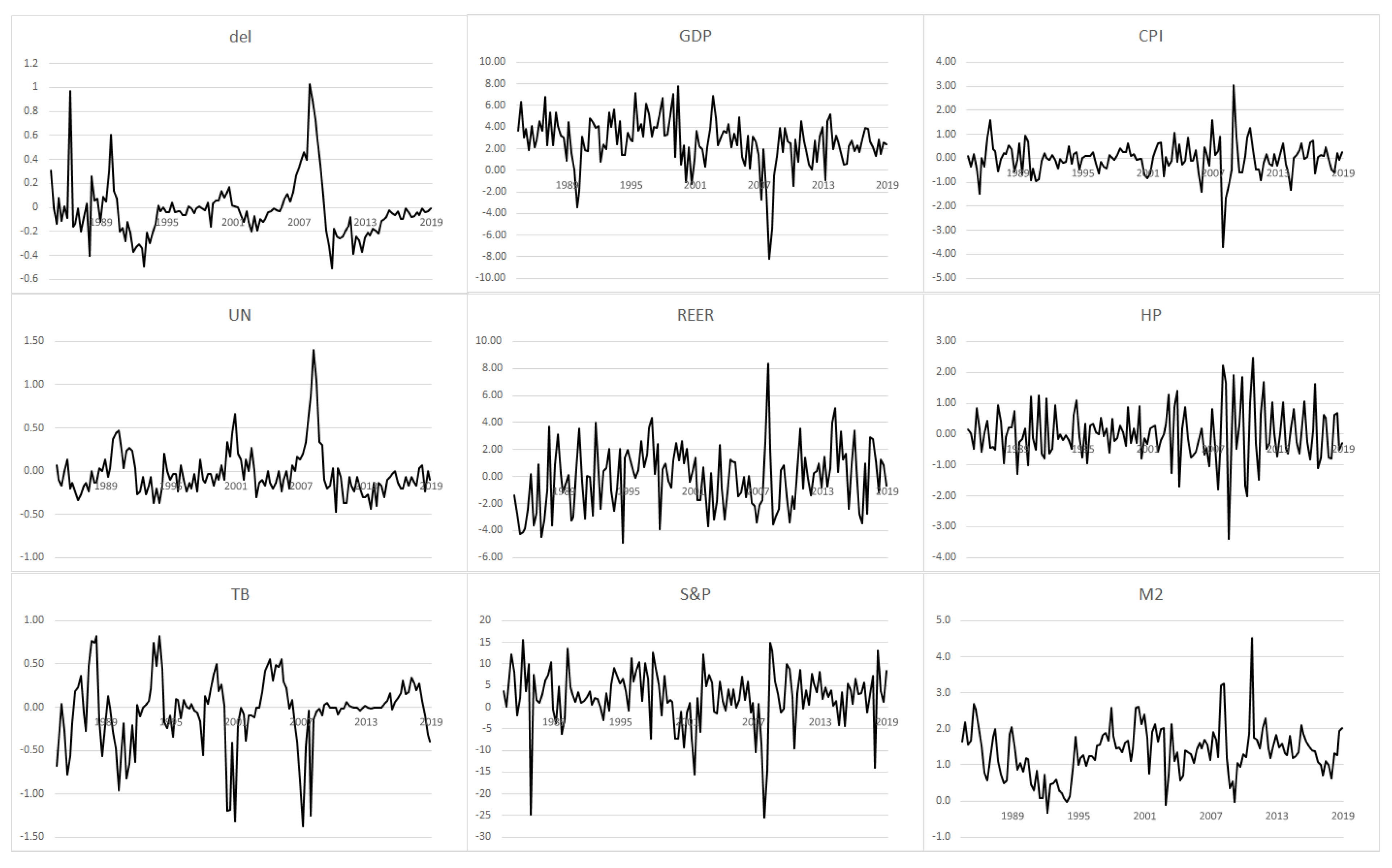
All variables are expressed as quarter-by-quarter percentage variations and are stationary, verified with an Augmented Dickey-Fuller (ADF) test. All the p-values of the ADF statistic are less than 0.001; the only exception is the statistic referring to $del$, but its p-value is only 0.002.10

In Figure 1, we illustrate the profile of the nine variables. All the macroeconomic variables present peaks at the end of 2008 and beginning of 2009: negative for $GDP$, $CPI$, $TB$, and $S\&P$, but positive for $UN$, $REER$, and $M2$. $HP$ shows more erratic behaviour. Similar trends hold in terms of the early 1990s recession, in particular for $GDP$ (negative peak), $TB$ (negative peak), and $UN$ (positive peak). These two subperiods correspond to the spans with the largest increases in the delinquency rates.

In

Table 2. Descriptive statistics of $del$ and other 8 macroeconomic variables, and correlations between $del$ and each macroeconomic variable for different time spans. The last two rows contain the orders of the ARMA models identified with the AIC criterion.

	del	GDP	CPI	UN	REER	HP	TB	S&P	M2
Mean	−0.02	2.62	−0.01	−0.03	−0.14	0.00	−0.05	2.31	1.36
Median	−0.04	2.70	0.01	−0.10	0.17	−0.08	−0.01	3.06	1.30
Minimum	−0.51	−8.20	−3.70	−0.47	−4.88	−3.39	−1.38	−25.52	−0.30
Maximum	1.03	7.80	3.06	1.40	8.36	2.48	0.82	15.59	4.50
st. dev.	0.24	2.29	0.69	0.27	2.31	0.85	0.40	6.63	0.71
Skewness	1.77	−1.09	−0.49	2.13	0.29	−0.06	−0.88	−1.28	0.58
Kurtosis	5.00	3.73	7.65	7.23	0.22	1.58	1.86	3.48	2.24
corr II 85–IV 19		−0.46	−0.10	0.65	0.01	0.03	−0.29	−0.18	0.21
corr II 85–III 90		−0.18	0.31	0.13	0.01	0.27	−0.07	0.20	−0.04
corr IV 07– II 09		−0.79	−0.96	0.81	0.67	0.38	0.03	−0.44	0.80
AR Order	2	2	2	3	2	2	3	1	2
MA order	0	0	2	2	2	0	3	0	1

, we show the main descriptive statistics of the nine time series. Only $GDP$, $SP$, and $M2$ show a mean of their quarter-by-quarter variation clearly different from zero and positive, whereas the first two have the largest variability with the largest peaks and troughs. Also, $GDP$ and $SP$ show a clear negative asymmetric pattern, caused by the strong effects of the recession and turmoil periods; for the same reason, $del$ and $UN$ show a positive asymmetry. The last part of the Table shows the sample correlation coefficients for the full time series and for two subperiods: the growth period before the early 1990s recession (II quarter 1985–III quarter 1990) and the crisis period due to the subprime mortgage crisis (IV quarter 2007–II quarter 2009).11 It is clear that the crisis period caused an increase (in some cases very large) in correlations with respect to the growth period and that the full correlation is in an intermediate position. This result is well known in financial time series, where correlations increase in correspondence to turmoil periods (see, Bauwens and Otranto 2016). These stylized facts support the idea to estimate the time-varying series of correlations for each pair of variables (delinquency rate & macroeconomic variable) to verify whether the correlation varies along time or is constant and if it presents particular abrupt changes in the correlation dynamics for the time span considered.

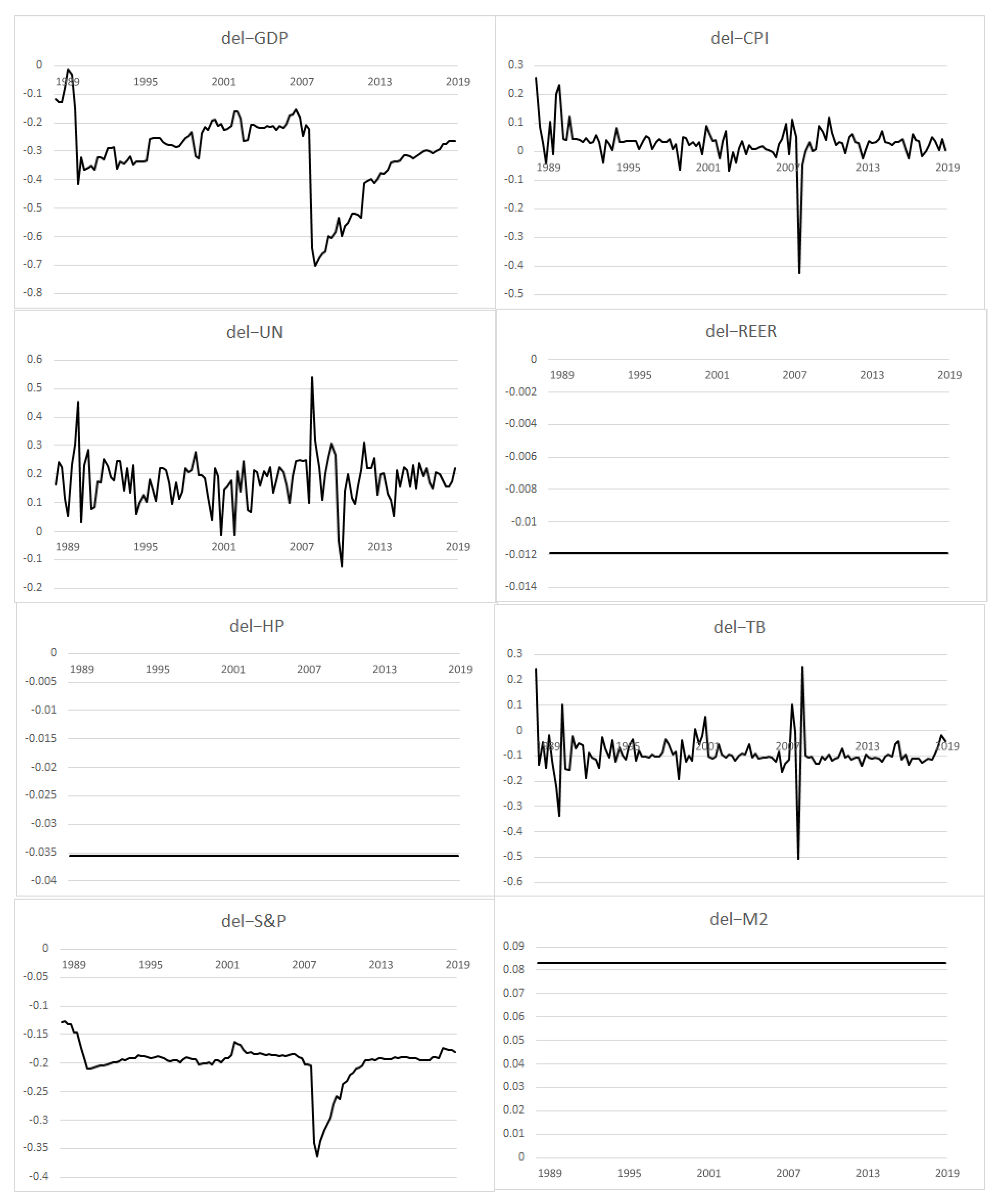
Before we proceed with the application of dynamic conditional correlation models, we need to clean the original series from their conditional mean ${\mathit{\mu }}_t$ in (1) to obtain the so-called demeaned series. We adopt ARMA models, choosing the order according to the Akaike Information Criterion (AIC), which performs relatively well for small samples (Hurvich and Tsai 1990). The bottom part of Table 2 shows the optimal model orders for each series. Denoting with ${\widehat{\mu }}_{i,t}$ the estimated values of variable i obtained by the corresponding ARMA model, the demeaned variable is obtained as ${\widehat{\epsilon }}_{i,t}=y_{i,t}-{\widehat{\mu }}_{i,t}$. We estimate the bivariate GARCH-DCC model (2)–(4) on these time series to obtain the series of the conditional correlation for each paired delinquency rate-macroeconomic variable.

4.2. Estimation of Variances and Correlations

Before estimating the GARCH-DCC models, it is necessary to verify if the demeaned series are heteroskedastic; otherwise, the GARCH part of the model does not make sense. The Engle (1982) test rejects the hypothesis of homoskedasticity only for $CPI$, $UN$, and $TB$, so we consider the GARCH part—Equation (2)—only for these variables. Moreover, the coefficients a and b of the DCC part—Equation (4)—are either equal to zero or not significant for the pairs $del$-$REER$, $del$-$HP$, and $del$-$M2$; this is evidence for constant correlation in the span considered. This is confirmed by a likelihood ratio (LR) test to compare the DCC model against the Constant Conditional Correlation (CCC–Bollerslev 1990); the latter is obtained by putting, in (4), $a=b=0$ and, as a consequence, ${\mathit{R}}_t=\overline{\mathit{R}}$. The last row of

Table 3. Estimation of the bivariate GARCH-DCC models (standard errors in parentheses) and Likelihood Ratio statistics to compare DCC and CCC models. The GARCH coefficients refer to the macroeconomic variable.

	$\mathit{del}$-$\mathit{GDP}$	$\mathit{del}$-$\mathit{CPI}$	$\mathit{del}$-$\mathit{UN}$	$\mathit{del}$-$\mathit{TB}$	$\mathit{del}$-$\mathit{S}\&\mathit{P}$
$\omega$		0.017	0.007	0.003
		(0.001)	(0.003)	(0.001)
$\alpha$		0.213	0.124	0.299
		(0.028)	(0.045)	(0.024)
$\beta$		0.717	0.589	0.688
		(0.029)	(0.165)	(0.025)
a	0.058	0.511	0.747	0.678	0.012
	(0.005)	(0.026)	(0.007)	(0.010)	(0.004)
b	0.937	0.000	0.000	0.000	0.886
	(0.007)	(0.013)	(0.001)	(0.015)	(0.272)
$LR$	37.94	16.18	13.65	14.74	208.36

shows the value of the LR statistics, to be compared with the critical value of a chi-squared distribution with 2 degrees of freedom (5.99 for a 5% significance level). We do not reject the null of constant correlation in these three cases,12 whereas it is rejected for the remaining five pairs. The results of the estimation of the bivariate GARCH-DCC models for the five pairs with time-varying correlation are shown in Table 3. Notice that the parameter b in pairs containing $CPI$, $UN$, and $TB$ is equal to zero; this means that the correlation can change only in terms of changes in the macroeconomic variable. Specifically, these relationships exhibit minimal time-varying movements that only depend on the sensitivity of correlations to the arrivals of news, represented by ${\mathit{u}}_{t-1}$ in (4). For the $GDP$ and $S\&P$, the presence of a large parameter b provides a time-varying but smooth dynamics of the correlation.

4.3. Empirical Results

Figure 2 shows the dynamics of the estimated conditional correlations obtained from the DCC model.13 A visual inspection of the figure highlights the presence of three patterns: constant conditional correlation, present in the correlations of $del$ with $REER$, $HP$, and $M2$; conditional correlations depending on news, characterizing the dynamics of the correlation of $del$ with $CPI$, $UN$, $TB$; persistent conditional correlation, present in the pairs $del$-$GDP$ and $del$-$S\&P$.

The first pattern shows that the correlation between $del$ and each one of the three variables is constant and close to zero in the full span considered. It seems that these three variables lack common dynamics with delinquency rates. This result is consistent with the behaviour detected in Table 1. In fact, if we exclude the subprime mortgage crisis, the variables $REER$ and $HP$ show a zero correlation in the full span considered, and $REER$ and $M2$ show a zero correlation in the period before the early 90s crisis. A possible interpretation of the absence of any correlation between the money supply and currency rate with the delinquency rate can be the combined effect of the “exorbitant privilege” and the self-explanatory impact that an increase in the money supply should produce on the enhancement of borrower solvency. As a matter of course, the US dollar’s role as international reserve currency calls for the Federal Reserve to support the world financial system during a crisis. Actually, a global slowdown determines a flight to safety, and consequently, the US dollar tends to be countercyclical, growing stronger during a global recession. In conjunction with the internal factors of a worsening in delinquency during a downturn, this effect can explain the described impact in the correlation behaviour. Our result of a zero correlation suggests that the two opposing forces end up to balance out. This result is a sort of middle ground between the positive (e.g., Klein 2013) and negative (e.g., Beck et al. 2015) correlation found in literature.

The puzzling interpretations and mixed results on the relationships among NPLs and $HP$ occurring in the literature (e.g. Dell’Ariccia and Marquez 2006; Wan 2018), which highlight the need for additional specification to appreciate them, makes unsurprising the result of our estimation for the same dynamic correlation.

The second pattern is obtained for the pairs presenting a b coefficient equal to zero (see Table 3); in this case, the correlation does not depend on its last value, but only on the news about the co-movements between the two variables under study. It is interesting to notice that the pairs $del$-$CPI$ and $del$-$TB$ show a clearly non-zero correlation only in regard to the two main economic shocks of the period 1985–2019: the early 1990s recession and the global recession of 2007–2010. In this last case, the correlation of both pairs switches to −0.4 for just one period. This behaviour could be interpreted as a spurious correlation due to jumps in all economic variables. Alternatively, the evidence can be the key to explaining the conflicting results between the delinquency rate and inflation, often found in the literature and already reported in a previous section (Ghosh 2017; Nkusu 2011; Radivojević et al. 2019). In general, during slump times, central banks adopt more active behaviour to support economic activities, but our findings show that in periods of a deep recession, this policy has a limited effect. Similarly, since the $TB$ series refers to short-term debt obligation with maturity shorter than a year, the $del$-$TB$ correlation has a more sensitive pattern in the troubled time of a recession, when central bank interventions usually involve money market products. In fact, our evidence corroborates the insight by Messai and Jouini (2013) that the ability of high interest rates to expand NPLs mainly applies to floating-rate loans, which are in turn closely related to money-market instruments. Different interpretations could be made for the correlation between $del$ and $UN$; it is often large and positive in the full span considered, as shown in most empirical findings in the literature (see Section 2). The higher correlation during the subprime mortgage crisis confirms the insight of a different impact of unemployment rate on NPLs depending on the different phase of growing or recession in the business cycle (Climent-Serrano 2019).

The most interesting pattern is the third one, with the correlations of $del$ with $GDP$ and $S\&P$ showing a strong persistence. The persistence of this correlation can be measured as $a+b<1$; in the $GDP$ case, this persistence is very high, near 1, whereas in the $S\&P$ case, it is around 0.9. In both cases, they are higher than the three cases of the second pattern, where the persistence is given by a (because $b=0$) and ranges between 0.51 and 0.75. The pair $del$-$GDP$ shows the highest correlation levels; after the first period with low correlation (near zero), there is an initial jump to a correlation of −0.4 for the early 1990s recession; then the correlation moves slowly toward lower levels between −0.3 and −0.2. There is another abrupt change in the last quarter of 2008, exceeding the level of −0.7. After this date, the correlation again reduces slowly toward the level of −0.3. Different behaviour is shown by the pair $del$-$S\&P$; in this case, the correlation is sufficiently constant after the shock in 1990 and is around −0.2. The only peak is in terms of the subprime mortgage crisis with a maximum (in absolute terms) of −0.36 in the first quarter of 2009. These results are also consistent with most studies involving these variables (see again Section 2), but we find a clear increase in correlation for the deepest economic recessions and financial crises, confirming our hypothesis of non-constant correlations. Despite a clear time-varying trend, correlations are still negative in all the span periods considered. This result is in line with the literature, which indeed does not identify conflicting views regarding the effect of the two variables on NPLs. Again, our results provide evidence that the phases of the business cycle do not affect NPLs symmetrically since an economic slowdown raises them more than the expansion reduce, according to Quagliariello (2007). Our result confirms the negative correlation between stock price and NPLs, but we have a clear increase during the greatest financial crisis in the considered time span.

4.4. Three-Variate Analysis

As we have said, the correlations between $del$ and each other macroeconomic variable follow different dynamics, which a multivariate DCC model cannot capture. Let us focus on the variables that seem more correlated to $del$ and with a clear pattern ($GDP$ and $S\&P$). 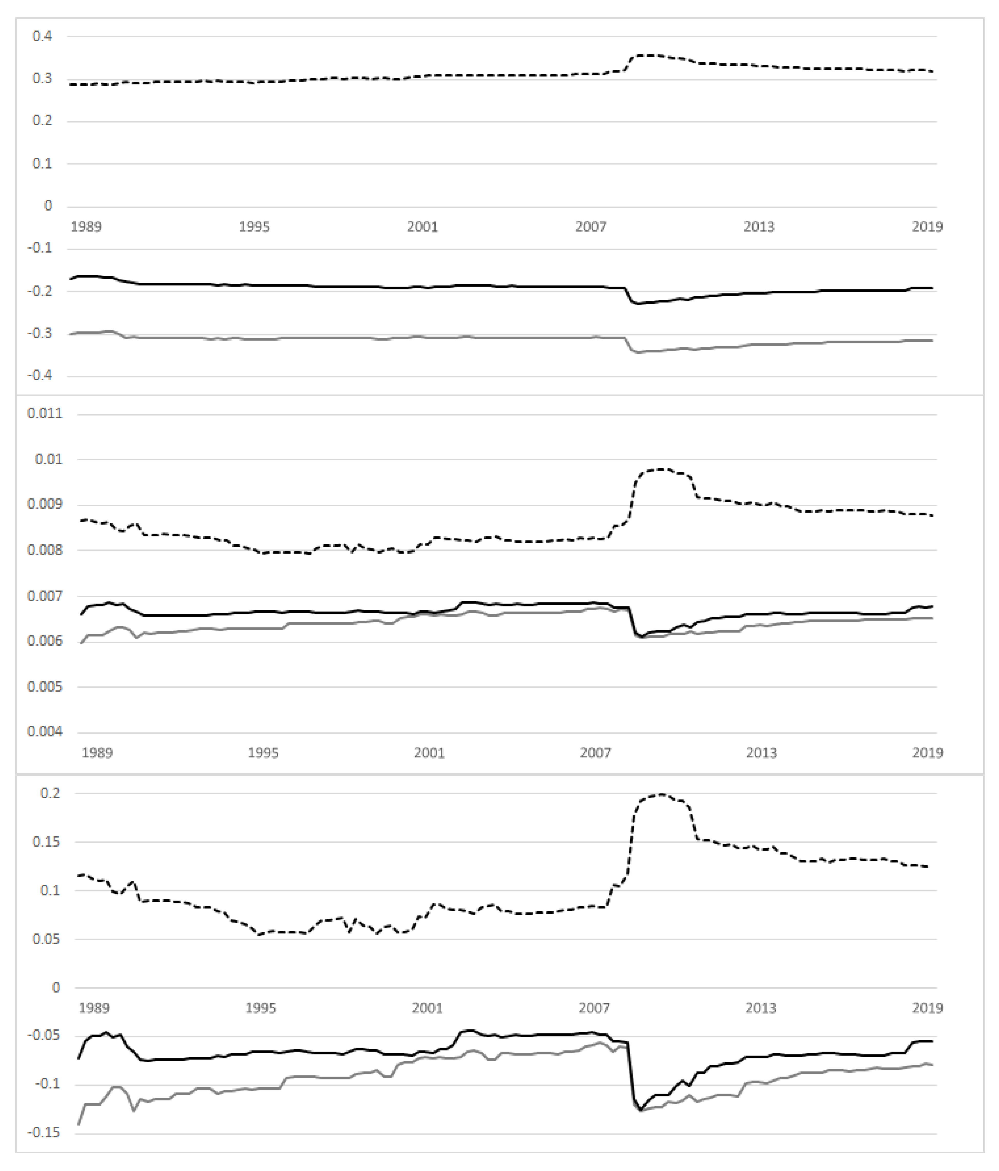From Table 3, it is clear that the dynamic correlation parameters a and b are different, so a 3-variate DCC model using the same coefficients a and b for all pairs could be misleading. In the top panel of Figure 3, we show the three dynamic conditional correlations derived from this DCC model; the estimated parameters are shown in

Table 4. Estimation of 3-variate DCC and NLARC models (robust standard errors in parentheses). The variables are $del$, $GDP$, $S\&P$.

Parameters	DCC	NLARC
a	0.002	0.032
	(0.000)	(0.005)
b	0.961	0.968
	(0.001)	(0.001)
${\varphi }_A$		1.458
		(0.059)
Log-lik	−3389.09	−3286.27

.

It is clear that the three lines follow similar dynamics, just with different signs (negative for the correlations involving $del$, positive otherwise). Moreover, the behaviour is almost constant, with only small movements corresponding to the subprime mortgage crisis, whereas the early 1990s recession seems to have no effect. This example shows the drawback of this kind of approach: it is very useful analyzing financial markets, where the co-movements between assets and markets is proven by stylized facts, but not in a macroeconomic framework, where the variables have proper dynamics. On the other hand, it would be useful to perform a multivariate analysis with more than two variables; the high correlations between pairs of variables could be overestimated because no other variables are considered in the study. In row terms, there is a sort of parallelism in the difference between correlations and partial correlations. A model that is not affected by this drawback is NLARC, illustrated in Section 3. In fact, it provides a set of time-varying coefficients, different for each time-varying correlation.

In the last column of Table 4, we show the estimation of the parameters for the NLARC model. The DCC model is nested in the NLARC model (the former can be obtained from the latter by setting ${\varphi }_A=0$), so it is possible to compare them by an LR test. It is also possible to derive, from the values of the log-likelihoods in Table 4, an LR statistic equal to 205.64, so the NLARC model outperforms the DCC.

The b coefficient of the NLARC is similar to the DCC case, whereas the time-varying a coefficients are shown in the middle panel of Figure 3 for each dynamic conditional correlation series. It is clear that the correlation between $GDP$ and $S\&P$ follows a different dynamic (different coefficient a) with respect to the other two correlations, which have similar parameters. Moreover, the parameter a decreases until 1995, with a small peak at the beginning of 1991 for the correlation of $GDP$-$S\&P$, increasing for the correlations $del$-$GDP$ and $del$-$S\&P$, and in the period 2007–2010, where an increasing bump is shown for $GDP$-$S\&P$ but the other two correlations decrease.

This behaviour is reflected in the correlation dynamics illustrated in the bottom panel of Figure 3. The differences with respect to the corresponding lines in Figure 2 and the corresponding 3-variate analysis with DCC (Top panel of Figure 3) are clear: the correlations are not constant, and they are close to zero, except for 1990–1991 and 2007–2010. In general, the correlation between $GDP$ and $S\&P$ seems to have smoother dynamics; the correlations of these two variables with $del$ are similar, but the pair $del$-$S\&P$ seems to have a constant correlation near zero, excluding the two recession sub-periods, where there are abrupt changes. The pair $del$-$GDP$, after each shock, shows a gradual return to lower levels of correlation.

In practice, the delinquency rates are clearly linked to the real and financial economy only in the case of strong crises. The early 1990s crisis seems to have had a small effect on delinquency rates than the subprime mortgage crisis, which shows the largest correlation period with a certain persistence of this effect; this aspect was not captured from the bivariate and DCC approaches.

5. Conclusions

In this paper, we have conducted an empirical exercise on a proxy of US non-performing loans (US bank delinquency rates) and eight macro-financial variables, to verify the presence of a non-constant pattern of correlations. Unlike the empirical papers present in the literature on this topic, we do not consider a fixed correlation or a correlation depending on the phases of the business cycle, determined a priori, instead of using two models (DCC and NLARC), both developed for the analysis of correlations between financial assets or markets, to provide data-driven patterns. Our purpose is not to establish the relationships between NPLs and macro-financial variables or the sign of such correlations, but to underline that this linkage is not constant over time and it depends strongly on particular events common to all economic variables. In practice, models estimating the dependence of NPLs on economic variables can be strongly affected by the time span adopted and particularly by the presence of negative economic periods. However, the effect of these periods is not the same across time, and correlations can also show clear jumps in their patterns. In particular, we demonstrate that the recent NLARC model, thanks to its flexible parameterization, is a promising method to capture different structures of correlations along time and different dynamics of correlations referring to different pairs of variables.

In our exercise, we distinguish three different patterns. Our findings confirm the insight that some variables ($M2$, $REER$, and $HP$) present almost zero correlation with the NPLs, which mediates the conflicting results about the sign of the correlations between these variables in the empirical literature.

Other correlations (the pairs $del$-$CPI$ and $del$-$TB$) take values different from zero only during the two main economic downturns covered in our sample period. Even if such a trend is consistent with a spurious correlation, it shows that the more proactive initiatives of the central banks in times of trouble are not able to fully counteract the negative dynamics of NPLs during crises. Therefore, this outcome can explain the contradictory findings found by previous studies and support the adoption of adequate time-varying models to explain NPLs by means of macroeconomic variables. The large and positive correlation estimated for the variables $del$ and $UN$, confirming empirical findings in the previous literature, seems to indirectly emphasize the accuracy of this insight.

The most interesting feature in our estimations is the persistent correlation path between the series $GDP$ and $S\&P$ with $del$. This evidence led us to carry out a more sophisticated tri-variate model, again with parameters changing over time. The results strongly confirm our belief that the delinquency rate is only closely related to real and financial economy indicators in the case of a strong crisis. Against this background, we take the view that proper analysis of the variables we have considered should apply a time-varying framework. Additional research is required to determine whether our outcome also holds when considering the delinquency rates for different categories of borrowers (households, large companies, small and medium enterprises, etc.) and other kinds of loans.

Our approach could be conveniently used in the selection of variables that affect NPLs, include them as explanatory variables, and select the time interval in which they could affect the dependent variable. This method should support the usual preliminary visual inspection to help in specifying the model. In particular, they might suggest using fixed or time-varying coefficients in the model for each selected exogenous variable.

An interesting extension of the DCC model, the Asymmetric (A)DCC proposed by Cappiello et al. (2006), could be adopted in this framework. This approach was developed again in the analysis of financial markets to consider the different effects when returns at time $t-1$ are negative or positive; see, for example, the application of Hou and Li (2016) to analyze the transmission mechanisms between U.S. and Chinese financial markets, and the inclusion of regime switching dynamics in ADCC models proposed by Pan et al. (2014) to explore the strategy on hedging crude oil using refined product. In our framework, the different signs could identify periods of growth and decline and improve our results.