
Testing the Efficiency of Globally Listed Private Equity Markets


Department of Business Administration and Information Sciences, University of Applied Sciences Merseburg, Eberhard-Leibnitz-Str. 2, 06217 Merseburg, Germany
J. Risk Financial Manag. 2021, 14(7), 313; https://0-doi-org.brum.beds.ac.uk/10.3390/jrfm14070313
Submission received: 31 May 2021
/
Revised: 28 June 2021
/
Accepted: 6 July 2021
/
Published: 8 July 2021
(This article belongs to the Special Issue European Financial Market Efficiency: Investors' Behaviour, Efficient Market Hypothesis and Behavioural Finance)
Abstract
:This study is the first to investigate the efficient market hypothesis in its weak form and the random walk behaviour of globally listed private equity (LPE) markets represented by nine global, regional, and style indices based on weekly data covering the period from January 2004 to December 2020. Autocorrelation tests, variance ratio tests, and a non-parametric runs test are employed. The results of the autocorrelation tests and the variance ratio tests tend to correspond for all indices, and they reject the random walk hypothesis for the returns of all LPE indices under investigation. In contrast, the runs test for direct weak-form market efficiency cannot reject the null hypothesis of a random walk process for almost all LPE indices under investigation. Furthermore, there is no evidence that the market efficiency of globally listed private equity markets has improved after the global financial crisis. Due to the fact that the rapidly growing asset class of LPE as a form of private equity is still relatively unknown, the implications of the results of our paper are relevant for investors, policy makers, and academics alike. In addition, the results provide valuable insights to better understand the emerging asset class of LPE.
JEL Classification:
G14; G151. Introduction
Private equity is one of the most important asset classes within the domain of alternative investments. In this context, listed private equity vehicles (LPE) have also become increasingly important as an alternative to investments in unlisted (traditional) private equity (Cumming et al. 2011; Brown and Kraeussl 2012). Due to the listing on a stock exchange, LPE offers high levels of liquidity for a generally illiquid asset class (Brown and Kraeussl 2012; Huss and Zimmermann 2012). Against this background, it is easy to understand why LPE has experienced a strong increase in demand from private and institutional investors. However, this rising interest in investment opportunities in LPE has raised questions in relation to the efficiency of LPE markets. The efficient market hypothesis (EMH) is one of the key cornerstones of finance, developed by Fama (1970). A market is called efficient if prices fully reflect all available information. Fama (1970) distinguishes three forms of efficiency depending on the information set considered. The most commonly examined form is the weak form, where a market is said to be weak-form efficient if investors cannot use past information to predict future returns. The semi-strong form asserts that prices reflect all publicly available information. Finally, the strong form asserts that prices reflect all available information, both public and private. Market efficiency is critical for investors because it gives them confidence in the fairness of market valuations. The weak-form EMH has been examined substantially in the literature for many traditional financial assets (e.g., Lim and Brooks 2011 for stocks; Zunino et al. 2012 for bonds). Similar studies have been undertaken for alternative investments, such as real estate investment trusts (REITs) (e.g., Schindler et al. 2010; Schindler 2011), commodities (e.g., Kristoufek and Vosvrda 2014), bitcoin (e.g., Urquhart 2016), and art (e.g., David et al. 2013). However, weak-form efficiency within the meaning of Fama (1970) has not been investigated for the LPE markets. Nonetheless, it should be noted that two studies have been carried out regarding the seasonal return patterns of LPE. Bauer et al. (2001) examined a sample of 229 LPE companies during the period from 1986 to 2000. They found evidence that almost all annual returns were achieved in the first six months of the year. They attributed this half-year effect to the fact that LPE companies publish their annually audited reports in the first half of the year. In addition, Bachmann et al. (2019) examined the so-called “sell in May” effect on global LPE markets. They found limited statistically significant evidence for the “sell in May” effect. In particular, the authors observed a statistically significant “sell in May” effect if they took time-varying volatility into account. These findings indicate that the “sell in May” effect is driven by time-varying volatility. It is surprising that LPE markets have not yet been studied for weak-form efficiency, given that LPE is a fast-growing asset class that is increasingly the focus of institutional and private investors. Therefore, we intend to fill this gap and apply a series of three powerful tests for weak-form efficiency and random walk behaviour to avoid spurious results and capture the full dynamics in LPE markets. Firstly, we examine the autocorrelation of returns which are assessed via the Ljung-Box test (Ljung and Box 1978). Secondly, we employ different variance ratio tests (Lo and MacKinlay 1988; Chow and Denning 1993), which are the most prevalent tests for testing stock markets for random walk behaviour. Finally, we use the runs test (Wald and Wolfowitz 1940), one of the most popular methods for investigating the weak form of market efficiency.
Because LPE as a form of private equity is, to date, relatively unknown among both investors and academics (e.g., Döpke and Tegtmeier 2018; Bachmann et al. 2019), this paper provides valuable insights for a better understanding of LPE as an emerging asset class and makes a significant contribution to expanding the LPE literature. The article proceeds as follows: Section 2 provides a short overview of the LPE market. Section 3 explains the methodology. Section 4 describes the database and the descriptive return statistics. Section 5 presents the empirical results. Section 6 summarizes and discusses the results.
2. The Listed Private Equity Market
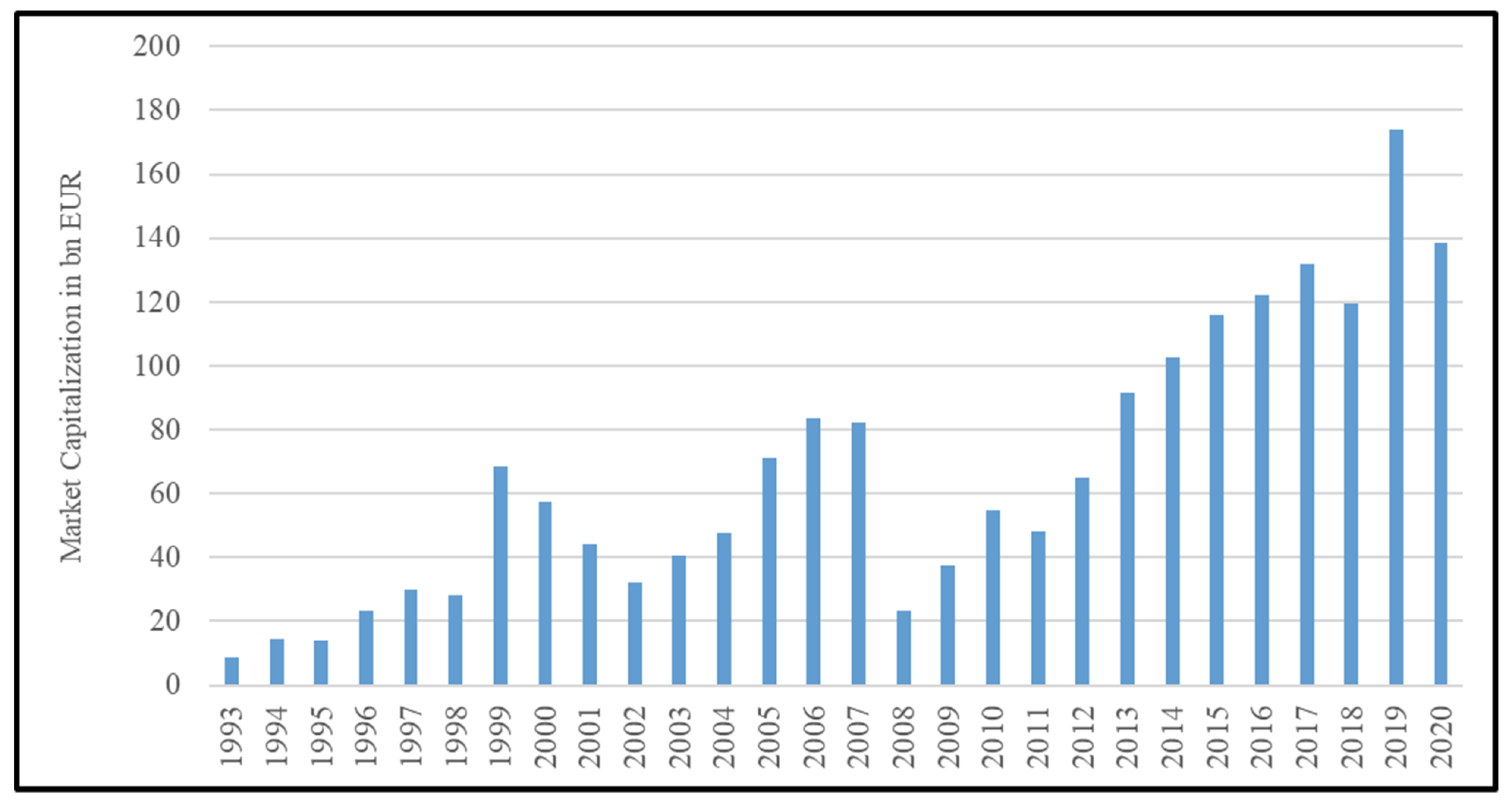
There are basically two ways to invest in private equity (Brown and Kraeussl 2012). Usually, investments in private equity are made through unlisted limited partnership funds (LPFs). These consist of a general partner (GP), who is the manager of the private equity fund and makes the investment and operating decisions, and limited partners, who are the passive investors in the fund and who do not make operating and investment decisions. This type of private equity investment was traditionally offered to institutional investors in the form of private placements. Parallel to the steady growth of the institutional private equity market, an increase in private equity funds (and funds of funds) listed on stock exchanges was observed. These LPE funds offer—in addition to institutional investors—public or private investors access to an asset class normally reserved for institutional investors. LPE funds, therefore, offer investors indirect exposure to traditional unlisted private equity. Differences between LPFs and LPE funds mainly relate to the heterogeneity of the organizational structure, which can be considered to be predominantly legal (Huss and Zimmermann 2012; Döpke and Tegtmeier 2018). In contrast, traditionally unlisted private equity is usually structured as LPFs. With regard to LPE, three main types can be distinguished.1 The most common form of LPE includes the direct LPE companies, which acquire and hold direct investments in companies. This can either be done from their own funds or in cooperation with limited partnerships managed by the company. Investors who invest in direct LPE companies are able to exactly break down which companies they are indirectly involved in and how they are valued. This makes it the most transparent type of investment in the LPE segment. Listed indirect private equity refers to companies that are not directly involved in private equity deals, but invest as a limited partner in cooperation with a general partner, often managed by an external private equity manager. Shareholders of indirect LPE companies, therefore, own shares in a portfolio of limited partnerships, making this form comparable to a fund of funds. The main advantage of such indirect vehicles for the investor is their broad diversification. Investors also gain access to private equity funds that would not be available to them without the network of relationships characteristic of fund of funds management and because of the high minimum investments required. However, there is an additional cost level and less transparency of the assets contained in the fund. The rarest type is called an LPE fund manager. This is a listed general partner, i.e., a management company that generates fees from a large number of limited partnerships. Shareholders, therefore, have no, or only very indirect, holdings in private equity portfolio companies. Investors should bear in mind that such companies are not always active only in the private equity segment, but may also be active in other business areas. The companies’ private equity exposure may be diluted accordingly. The market capitalization of global LPE markets has risen continuously during the past ten years. Figure 1 shows the market capitalization of LPE as measured by the LPX Composite index, which contains all LPE companies globally that fulfil certain liquidity requirements.2
In 1993, the global market capitalization of LPE was EUR 8.9 bn. At the end of the 1990s, there was a significant boom in LPE listings (Bilo et al. 2005), which explains the sharp increase in LPE market capitalization until 1999. The global market capitalization of LPE in 1999 was EUR 68.58 bn. When the dotcom bubble burst in 2000, a decline in market capitalization was observed until 2002. The following years were characterized by high growth, which lasted until 2007. The sub-prime financial crisis of 2008–2009 curbed these developments. In 2008, the global market capitalization was EUR 23.41 bn., followed by a market capitalization of EUR 37.69 bn. in 2009. Thereafter, sustainable growth followed, which reached its peak at the end of 2019, with a global market capitalization of LPE of EUR 174.14 bn. At the end of 2020, the global market capitalization of LPE was EUR 138.72 bn. This decline—compared to 2019—was primarily caused by the global COVID-19 pandemic and the accompanying decline in valuations.
3. Methodology
The objective of this paper is either to support, or debunk, the hypothesis that the global LPE markets are efficient, which implies that they follow random changes in stock prices. The focus is specifically on the EMH in its weak form because this has not been studied for LPE to date. Moreover, there is no reason to study the semi-strong (and/or strong) form before the weak form can be demonstrated based on empirical tests (Wong and Kwong 1984; Fawson et al. 1996). In addition, as described in detail in Section 4, the empirical investigations are based on indices and their returns. Information on individual companies and their performance is not included. Similarly, there is no information on the performance of individual fund managers or data on insider trading, which is why no additional studies have been conducted on the semi-strong or strong form.
The EMH implies in its weak form that stock price changes are unpredictable (Fama 1970). A commonly used test of market efficiency is to investigate whether a stock price follows a random walk. According to the random walk hypothesis, the behaviour of stock price changes can be described by an unpredictable random process. This states that the actual stock price is equal to the previous price plus the realization of a random variable, which can be written as:
where denotes the natural logarithm of a stock price and denotes a random disturbance term at time t, which fulfils and , for all t. If the expected stock price movements are given by , the previous price of the stock is the best linear estimator for the stock price .
To investigate whether the individual series of different LPE indices follow random walks, we apply three tests. The first approach we use to test the weak-form efficiency is based on an investigation of the interrelationship between current and past returns. For this purpose, we consider the autocorrelation structure of the respective LPE index returns under investigation and test the joint hypothesis that all autocorrelations are simultaneously equal to zero by using the Ljung and Box (1978) portmanteau statistic . The Ljung–Box -statistic is given by:
where denotes the jth autocorrelation and N is the number of observations. Under the null hypothesis that the first k autocorrelations are zero , the -statistic is distributed as chi-squared with degrees of freedom equal to the number of autocorrelations (k).
Secondly, we apply the variance ratio test developed by Lo and MacKinlay (1988), which is particularly useful for studying stock returns because they are commonly not normally distributed (Schindler et al. 2010). Corresponding to the methodology of Lo and MacKinlay (1988), if the natural logarithm of a stock price time series Pt is a pure random walk, then the variance of its q-differences grows proportionally with the difference q. If the stock return series follows a random walk, the variance of the qth difference would be equivalent to q times the variance of first differences. According to the random walk model, the variance of the first differences, denominated as and , respectively, increase linearly over time, so that the variance of the qth difference can be computed as:
For the qth lag in , where q is any integer greater than one, the variance ratio, , is then:
where denotes the unbiased estimator of the variance. The expected value of is equal to one under the null hypothesis of a random walk for all values of q. denotes the logarithmic price process and describes a q period’s continuously compounded return. The estimator of the hth serial correlation coefficient is given by . A variance ratio greater (less) than one indicates mean aversion (mean reversion). Under the assumption of a homoscedastic random walk hypothesis, Lo and MacKinlay (1988) developed an asymptotic standard normal test statistic for , which can be defined for a sample size of nq + 1 observations (P0, P1, …, Pnq) as:
where , and denotes that the distributional equivalence is asymptotic.
Due to the fact that the variance of most stock returns is often conditionally heteroscedastic with respect to time, Lo and MacKinlay (1988) present a second test statistic with a heteroscedasticity-consistent variance estimator :
with and .
However, the approach of Lo and MacKinlay focuses on a single variance ratio for an individual aggregation interval, q, by comparing the test statistics and with the critical value of the standard normal distribution. In contrast, the random walk hypothesis requires that = 1 for all q. A multiple variance ratio test was developed by Chow and Denning (1993). Consider a set of m variance ratio tests where , associated with the set of aggregation intervals . Under the random walk hypothesis, the multiple variance ratio tests will have several sub-hypotheses that will be tested jointly:
The rejection of any one or more H0i values leads to rejection of the random walk hypothesis. To facilitate comparison of this study with previous research (e.g., Lo and MacKinlay 1988; Campbell et al. 1997; Borges 2011; Jamaani and Roca 2015) on other markets, q values of 2, 4, 8 and 16 are selected. For a set of m Lo and MacKinlay variance ratio test statistics , the random walk hypothesis is rejected if any one of the is significantly different from one, so only the maximum absolute value in the set of test statistics is considered. The Chow and Denning (1993) multiple variance ratio approach is based on the Studentized Maximum Modulus (SMM) distribution and uses these critical values, rather than the critical values of a standard normal distribution, to test the null hypotheses:
where SMM (α; m; T) is the upper α point of the Studentized Maximum Modulus (SMM) distribution with parameters m (number of variance ratios) and T (sample size) degrees of freedom. Asymptotically,
where has a standard normal distribution with . The size of the multiple variance ratio test is controlled by comparing the calculated values of the standardized test statistics, either Z(q) or Z*(q), with the critical values of the SMM. If the maximum absolute value of, for example, Z(q), is greater than the critical value at a given significance level, the random walk hypothesis is rejected.
The variance ratio tests reveal that, due to factors such as autocorrelation or long-run dependence, some stock prices may not follow a random walk. However, none of these properties that violate the random walk hypothesis inevitably implies market inefficiency. Therefore, it is essential to employ a direct test of the market efficiency in a weak form. Whereas the parametric serial correlation test of independence implies normality of the returns, we employ, thirdly, a simple non-parametric runs test (Wald and Wolfowitz 1940) to analyse the weak-form efficiency of returns for the LPE indices under investigation. The runs test is another common test for investigating whether the index return series follows a random walk (Campbell et al. 1997) and does not require normality or a linear return-generating process. In applying the runs test, the number of runs, R, of negative and positive returns ( and respectively) are counted. The sampling distribution of R approximates normality if the total number of observations N (N = + ) is greater than 20. If this holds, the distribution of R has the mean or expected value of (Kleiman et al. 2002):
and a standard deviation of:
The test statistic for the null hypothesis that the returns are random is given by the Z-statistic, which can be written as follows:
The advantage of the runs test compared to test procedures based on correlations or covariances, such as the autocorrelation test, is that it is comparatively robust to strong short-term changes in returns; also, its results are not influenced by such effects. This makes the runs test particularly suitable as a supplement to the autocorrelation test for testing the random walk hypothesis.
4. Data and Preliminary Analysis
Our sample includes nine LPE indices provided by the LPX Group, and includes global, regional, and style indices. The LPX Group is a Swiss-based research house dedicated to alternative investments. The LPX listed private equity index family was the first set of benchmarks for private equity based solely on objective market valuations. Today, these indices are widely accepted as a reliable tool for valuation and representative performance benchmarks for (listed) private equity in both the academic community and among industry experts (Huss and Zimmermann 2012).3 Table 1 gives a detailed description of these indices.
All indices are calculated as total return indices, and, to limit the weight of individual constituents in the respective indices, a cap is set for the market capitalization of any single constituent of the relevant index. We apply returns continuously compounded on a weekly basis to each index, and our observation period stretches from January 2004 to December 2020. The reason for the choice of the observation period is that not all indices have the same history. For example, data for the LPX Mezzanine index are only available since January 2004. Given the fact that various investigations have shown that market efficiency has improved since the global financial crisis (e.g., Vieito et al. 2016; Gupta and Sankalp 2017), we also conduct robustness checks to investigate the behaviour of LPE returns before and after the 2008 financial crisis. For this purpose, we divide the observation period into two subperiods, with the pre-crisis period spanning January 2004 to December 2008 and the post-crisis period spanning January 2009 to December 2020.4 The regional indices are denominated in local currencies. In contrast, the global indices are denominated using USD. This denomination is applied because global indices are not calculated in local currencies. For all global indices, USD makes the highest currency contribution; hence, all global indices are denominated in USD.
Table 2 summarizes the characteristics of the weekly returns of the LPX indices under investigation. During the full period reported in Panel A, the weekly mean returns of the LPE indices range between 0.16% for the LPX Europe and 0.03% for the LPX Mezzanine. The highest weekly volatility of 4.33% appears for the LPX America, whereas the LPX UK has the lowest volatility of 2.56%. Within the pre-crisis period reported in Panel B, all indices have negative weekly average returns, ranging from -0.33% for the LPX Mezzanine to −0.11% for the LPX Direct. One of the reasons for this is the massive losses caused by the global financial crisis. The volatility within this period ranges between 4.64% for the LPX Mezzanine and 2.75% for the LPX UK. Within the post-crisis period reported in Panel C, weekly average returns range from 0.29% for the LPX Europe and the LPX Indirect to 0.18% for the LPX Mezzanine. The highest volatility within this period is shown by the LPX Mezzanine, of 4.28%, whereas the volatility for the LPX Indirect, of 2.28%, is the lowest. In addition, all indices have negative skewness and extreme kurtosis within all periods. Consequently, the Jarque–Bera test rejects the null hypothesis of a normal distribution at the 1% level for all indices within all periods under investigation.5
5. Empirical Results
Starting with the first methodological approach, Table 3 presents the results of the autocorrelation test.
Within the full period reported in Panel A, all indices—except the LPX America—have positive first-order autocorrelation coefficients. Moreover, the first-order autocorrelation coefficients for the LPX UK, the LPX Venture, and the LPX Indirect are significant at the 1% level and show a positive sign. Furthermore, all indices have positive and significant second-order autocorrelation coefficients at the 1% level. This is an indication of a general upward trend. In contrast, the higher-order autocorrelation coefficients show a cluster of negative signs, which are also significant at the 1% level. The predominantly positive autocorrelation up to the third order in the returns of the LPE indices may indicate the presence of a short-term profitable trading rule under which past winners are bought and past losers are sold. Moreover, these results are consistent with the findings of Poterba and Summers (1988), who also conclude in their analysis of stock markets that mean aversion processes are observed in the short run and mean reversion behaviour over longer time periods. Looking at the results for the pre-crisis period reported in Panel B and the post-crisis period reported in Panel C, the results for the full period tend to be confirmed. In this context, it is striking that the autocorrelation coefficients up to the fourth order during the pre-crisis period for the LPX America, the LPX Buyout, the LPX Venture, the LPX Direct, and the LPX Mezzanine show almost no significance. Comparing the results of the pre-crisis period with those of the post-crisis period, we find no evidence that market efficiency has improved since the global financial crisis. On the contrary, the results within the pre-crisis period tend to indicate higher market efficiency. These results are inconsistent with the evidence for stock markets, where there is evidence of an improvement in market efficiency after the global financial crisis (Vieito et al. 2016; Gupta and Sankalp 2017).
The positive autocorrelation of stocks and stock returns in short-term intervals is a well-known phenomenon in the literature, and may have different underlying causes. In their study, Lo and MacKinlay (1988) point to the types of risks present in individual stocks and in stock indices as possible causes. Like French and Roll (1986), they conclude in their research that stocks themselves have negative autocorrelations and stock indices have positive autocorrelations. The result of positive autocorrelations of indices is also predominantly true for LPE indices. Following the argumentation of Lo and MacKinlay (1988), this is associated with the high proportion of systematic risk in indices compared to stocks, which mainly contain idiosyncratic risk. The stronger presence of systematic risk in portfolios relative to unsystematic risk means that certain longer-term components of returns acting on markets have a stronger impact and then lead to positive autocorrelations.
Table 4, Table 5 and Table 6 report the results of the variance ratio test for the full period and the pre-crisis and the post-crisis periods. During the full period displays in Table 4, all indices exhibit a variance ratio less than one, indicating a mean reversion process.
Relying on the assumption of homoscedasticity, the test statistics for all indices are significant at the 1% level, and the null hypothesis of a random walk is rejected. When adapting the tests for heteroscedasticity, the results remain unchanged. However, the significance level at lag q = 16 for the LPX Buyout, the LPX Venture, and the LPX Indirect decreases from 1% to 5%. The simultaneous consideration of multiple lag lengths also leads to a rejection of the random walk hypothesis for all indices at the 1% significance level. The results for the pre-crisis period reported in Table 5, and the post-crisis period reported in Table 6, show similar results. In summary, this non-random walk pattern, based on the variance ratio test, is consistent with the serial correlation results. Comparing the results of the pre-crisis period with those of the post-crisis period, we again find no evidence that market efficiency has improved since the global financial crisis.
Non-autocorrelated asset returns do not necessarily indicate market efficiency (Lucas 1978; Summers 1986), in particular because of the skewness and kurtosis shown in the returns in Exhibit 3. To the extent that the return generation process is a non-linear one, the autocorrelation coefficient is not a robust measure for testing market (in)efficiency. To complement the autocorrelation test, we, therefore, use the runs test, which is a direct test of market efficiency in its weak form and is comparatively robust to strong short-term changes in returns. In addition, its results are not affected by such effects. Table 7 reports the results of the non-parametric runs test for independence between sequential events in time series. During the full period reported in Panel A, all indices except the LPX America, the LPX Buyout, and the LPX Mezzanine show negative test statistics. This suggests a mean aversion process, in which the number of observed runs is lower than the statistically expected number. In contrast to the previous test procedures, the null hypothesis of a random walk weak-form market efficiency cannot be rejected, with the exception of the LPX Indirect index. This also applies for the pre-crisis period reported in Panel B and the post-crisis period reported in Panel C. Furthermore, comparing the results of the pre-crisis period with those of the post-crisis period, no improvement in market efficiency after the global financial crisis can be observed.
6. Discussion and Conclusions
This paper is the first to investigate the efficient market hypothesis in its weak form and the random walk behaviour of global LPE markets represented by nine global, regional, and style indices based on weekly data covering the period from January 2004 to December 2020. Autocorrelation tests, variance ratio tests, and a non-parametric runs test are employed. In a comparison of results by the different test procedures, the results of the autocorrelation tests and the various variance ratio tests tend to correspond for all indices, and they rejected the random walk hypothesis for the returns of all LPE indices under investigation. In contrast, based on the runs test, the null hypothesis of a random walk process in respect of weak-form market efficiency cannot be rejected for all LPE indices under investigation. The only exception is the LPX Indirect index. Here, the null hypothesis of a random walk process in respect of weak-form market efficiency can be rejected for all periods under investigation at the 10% significance level. When comparing the pre-crisis period with the post-crisis period, no evidence was found that market efficiency improved after the global financial crisis.
Due to the fact that the rapidly growing asset class of LPE as a form of private equity is still relatively unknown (Döpke and Tegtmeier 2018; Bachmann et al. 2019), the implications of the results of our paper are relevant for investors, policy makers, and academics alike. For investors and portfolio managers, the non-random walk pattern and weak-form market efficiency in LPE markets suggest that short-term profitable trading strategies based on historical data cannot be developed. The finding of positive autocorrelation suggests predictability of returns. However, the demonstrated weak-form market efficiency based on the results of the runs test in these markets makes it unlikely that investors or portfolio managers could develop trading strategies to exploit predictability. If policy makers are better informed about the current efficiency status of LPE markets, they are in a better position to make decisions that promote the development of LPE markets and thus make them more efficient. Possible decisions and measures in this context could include increasing the flow of information for more transparency or expanding the digital infrastructure for better trading technologies. This should then lead to improved liquidity and a more efficient allocation of capital, which in turn should have a positive impact on economic growth. For academics, the results provide valuable insights to better understand the emerging asset class of LPE and the resulting questions for future research directions. In particular, in light of the mixed evidence between the results of the runs test, and the tendency for consistent results of the autocorrelation test and the variance ratio tests, further research on the market efficiency of global LPE markets is required. Because the focus of this paper was on weak-form information efficiency, future studies should focus on the semi-strong and strong information efficiency hypotheses. On the basis of comprehensive information regarding individual LPE companies, investigations of the semi-strong information efficiency hypothesis can be carried out, for example, with the help of event studies. Furthermore, using data on insider trading, it would be appropriate to investigate the strong information efficiency in LPE markets. As research in finance has increasingly focused on the behaviour of high-frequency data in recent decades, the availability of high-frequency data also opens up further research possibilities with respect to the analysis of the information efficiency of global LPE markets. For example, there is an opportunity to extend the results obtained in this paper to provide additional insights based on the heterogeneous market hypothesis (Dacorogna et al. 2001) using high-frequency data in combination with realized volatility estimators (Floros et al. 2020).
Funding
This research received no external funding.
Data Availability Statement
The data presented in this study are available on request from the corresponding author.
Acknowledgments
The author would like to thank Jörg Döpke for his helpful comments.
Conflicts of Interest
The author declares no conflict of interest.
| 1 | Detailed overviews of the forms of organization of LPE vehicles are given by Lahr and Herschke (2009) and Huss and Zimmermann (2012). |
| 2 | There are more than 300 LPE companies globally, of which around 120 fulfil the liquidity requirements of the LPX Group. |
| 3 | Detailed information about the LPX Group and the indices provided is given on the LPX Group website at https://www.lpx-group.com/index.php (accessed on 17 June 2021). |
| 4 | Since there is no consistent definition of the end of the pre-crisis period or the beginning of the post-crisis period in the literature, the period chosen here follows Vieito et al. (2016) and Drobetz et al. (2020). |
| 5 | In addition, we used the D’Agostino et al. (1990) test to perform an unreported robustness check. Again, the null hypothesis of a normal distribution can be rejected at the 1% level for all indices and study periods. Furthermore, the null hypothesis that the skewness is equal to 0 and the kurtosis is equal to 3 was tested. The null hypothesis was also rejected for all indices and study periods for both skewness and kurtosis at the 1% level. For the sake of brevity, the respective results are available upon request from the author. |
References
- Bachmann, Carmen, Lars Tegtmeier, Johannes Gebhardt, and Marcel Steinborn. 2019. The ‘Sell in May’ Effect: An Empirical Investigation of Globally Listed Private Equity Markets. Managerial Finance 45: 793–808. [Google Scholar] [CrossRef]
- Bauer, Michael, Stéphanie Bilo, and Heinz Zimmermann. 2001. Publicly Traded Private Equity: An Empirical Investigation. Working Paper. Basel, Switzerland: University of Basel. [Google Scholar]
- Bilo, Stéphanie, Hans Christophers, Michél Degosciu, and Heinz Zimmermann. 2005. Risk, Returns, and Biases of Listed Private Equity Portfolios. Working Paper. Basel, Switzerland: University of Basel. [Google Scholar]
- Borges, Maria Rosa. 2011. Random Walk Tests for the Lisbon Stock Market. Applied Economics 43: 631–39. [Google Scholar] [CrossRef] [Green Version]
- Brown, Christopher, and Roman Kraeussl. 2012. Risk and Return Characteristics of Listed Private Equity. In The Oxford Handbook of Private Equity. Edited by Douglas Cumming. New York: Oxford University Press, pp. 549–78. [Google Scholar]
- Campbell, John Y., Andrew W. Lo, and A. Craig MacKinlay. 1997. The Econometrics of Financial Markets. Princeton: Princeton University Press. [Google Scholar]
- Chow, K. Victor, and Karen C. Denning. 1993. A Simple Multiple Variance Ratio Test. Journal of Econometrics 58: 385–401. [Google Scholar] [CrossRef]
- Cumming, Douglas, Grant Fleming, and Sofia A. Johan. 2011. Institutional Investment in Listed Private Equity. European Financial Management 17: 594–618. [Google Scholar] [CrossRef]
- D’Agostino, Ralph B., Albert Belanger, and Ralph B. D’Agostino Jr. 1990. A Suggestion for Using Powerful and Informative Tests of Normality. American Statistician 44: 316–21. [Google Scholar]
- Dacorogna, Michel, Ulrich Müller, Richard Olsen, and Olivier Pictet. 2001. Defining Efficiency in Heterogeneous Markets. Quantitative Finance 1: 198–201. [Google Scholar] [CrossRef]
- David, Géraldine, Kim Oosterlinck, and Ariane Szafarz. 2013. Art Market Inefficiency. Economics Letters 121: 23–25. [Google Scholar] [CrossRef]
- Döpke, Jörg, and Lars Tegtmeier. 2018. Global Risk Factors in the Returns of Listed Private Equity. Studies of Economics and Finance 35: 340–60. [Google Scholar] [CrossRef]
- Drobetz, Wolfgang, Henning Schröder, and Lars Tegtmeier. 2020. The Role of Catastrophe Bonds in an International Multi-Asset Portfolio: Diversifier, Hedge, or Safe Haven? Finance Research Letters 33: 101198. [Google Scholar] [CrossRef]
- Fama, Eugene F. 1970. Efficient Capital Markets: A Review of Theoretical and Empirical Work. Journal of Finance 25: 383–417. [Google Scholar] [CrossRef]
- Fawson, Chris, Terry F. Glover, Wenshwo Fang, and Tsangyao Chang. 1996. The Weak-Form Efficiency of the Taiwan Share Market. Applied Economics Letters 3: 663–67. [Google Scholar] [CrossRef]
- Floros, Christos, Konstantinos Gkillas, Christoforos Konstantatos, and Athanasios Tsagkanos. 2020. Realized Measures to Explain Volatility Changes over Time. Journal of Risk and Financial Management 13: 125. [Google Scholar] [CrossRef]
- French, Kenneth R., and Richard Roll. 1986. Stock Return Variances—The Arrival of Information and the Reaction of Traders. Journal of Financial Economics 17: 5–26. [Google Scholar] [CrossRef]
- Gupta, Jyoti, and Sardana Sankalp. 2017. The Impact of Global Financial Crisis on Market Efficiency: An Empirical Analysis of the Indian Stock Market. International Journal of Economics and Finance 9: 225–52. [Google Scholar]
- Huss, Matthias, and Heinz Zimmermann. 2012. Listed Private Equity: A Genuine Alternative for an Alternative Asset Class. In The Oxford Handbook of Private Equity. Edited by D. Cumming. New York: Oxford University Press, pp. 579–610. [Google Scholar]
- Jamaani, Fouad, and Eduardo Roca. 2015. Are the Regional Gulf Stock Markets Weak-Form Efficient as Single Stock Markets and as a Regional Stock Market? Research in International Business and Finance 33: 221–46. [Google Scholar] [CrossRef]
- Kleiman, Robert T., James E. Payne, and Anandi P. Sahu. 2002. Random Walks and Market Efficiency: Evidence from International Real Estate Markets. Journal of Real Estate Research 24: 279–98. [Google Scholar] [CrossRef]
- Kristoufek, Ladislav, and Miloslav Vosvrda. 2014. Commodity Futures and Market Efficiency. Energy Economics 42: 50–57. [Google Scholar] [CrossRef] [Green Version]
- Lahr, Henry, and Florian T. Herschke. 2009. Organizational Forms and Risk of Listed Private Equity. The Journal of Private Equity 13: 89–99. [Google Scholar] [CrossRef]
- Lim, Kian-Ping, and Robert Brooks. 2011. The Evolution of Stock Market Efficiency over Time: A Survey of the Empirical Literature. Journal of Economic Surveys 25: 69–108. [Google Scholar] [CrossRef]
- Ljung, Greta M., and George E. P. Box. 1978. On a Measure of Lack of Fit in Time Series Models. Biometrika 65: 297–303. [Google Scholar] [CrossRef]
- Lo, Andrew W., and Craig MacKinlay. 1988. Stock Market Prices Do Not Follow Random Walks: Evidence from a Simple Specification Test. Review of Financial Studies 1: 41–66. [Google Scholar] [CrossRef]
- LPX Group. 2021. Available online: https://www.lpx-group.com (accessed on 17 June 2021).
- Lucas, Robert E. 1978. Asset Prices in an Exchange Economy. Econometrica 46: 1429–45. [Google Scholar] [CrossRef]
- Poterba, James M., and Lawrence H. Summers. 1988. Mean Reversion in Stock Prices. Journal of Financial Economics 22: 27–59. [Google Scholar] [CrossRef]
- Schindler, Felix. 2011. Market Efficiency and Return Predictability in the Emerging Securitized Real Estate Markets. Journal of Real Estate Literature 19: 111–50. [Google Scholar] [CrossRef]
- Schindler, Felix, Nico Rottke, and Roland Füss. 2010. Testing the Predictability and Efficiency of Securitized Real Estate Markets. Journal of Real Estate Portfolio Management 16: 171–91. [Google Scholar] [CrossRef]
- Summers, Lawrence H. 1986. Does the Stock Market Rationally Reflect Fundamental Values? Journal of Finance 41: 591–600. [Google Scholar] [CrossRef]
- Urquhart, Andrew. 2016. The Inefficiency of Bitcoin. Economics Letters 148: 80–82. [Google Scholar] [CrossRef]
- Vieito, João Paulo, Wing-Keung Wong, and Zhen-Zhen Zhu. 2016. Could the Global Financial Crisis Improve the Performance of the G7 Stocks Markets? Applied Economics 48: 1066–80. [Google Scholar] [CrossRef] [Green Version]
- Wald, Abraham, and Jacob Wolfowitz. 1940. On a Test Whether Two Samples are from the Same Population. Annals of Mathematical Statistics 11: 147–62. [Google Scholar] [CrossRef]
- Wong, K. A., and K. S. Kwong. 1984. The Behaviour of Hong Kong Stock Prices. Applied Economics 16: 905–17. [Google Scholar] [CrossRef]
- Zunino, Luciano, Aurelio Fernández Bariviera, M. Belén Guercio, Lisana B. Martinez, and Osvaldo A. Rosso. 2012. On the Efficiency of Sovereign Bond Markets. Physica A: Statistical Mechanics and Its Applications 39: 4342–49. [Google Scholar] [CrossRef] [Green Version]


Table 1.
Used LPX indices.
| Index | Description | Currency |
|---|---|---|
| LPX Composite | The LPX Composite describes the global performance of listed private equity companies. The index covers listed private equity companies with the highest levels of market capitalization and liquidity. The index is diversified across regions, private equity investment styles, financing styles, and vintages. | USD |
| LPX Europe | The LPX Europe describes the performance of private equity companies listed on a European stock exchange. The LPX Europe covers the 30 most highly capitalized and liquid companies and is diversified across private equity investment styles, financing styles, and vintages. | EUR |
| LPX UK | The LPX UK describes the performance of private equity companies listed on a UK stock exchange. The LPX UK covers the 30 most highly capitalized and liquid companies and is diversified across private equity investment styles, financing styles, and vintages. | GBP |
| LPX America | The LPX America describes the performance of private equity companies listed on a North American stock exchange. The LPX America covers the 30 most highly capitalized and liquid companies and is diversified across private equity investment styles, financing styles, and vintages. | USD |
| LPX Buyout | The LPX Buyout describes the global performance of listed private equity companies that pursue a buyout private equity investment strategy. The LPX Buyout covers the 30 most highly capitalized and liquid companies and is diversified across regions, financing styles, and vintages. | USD |
| LPX Venture | The LPX Venture describes the global performance of listed private equity companies that predominately provide venture capital. The LPX Venture covers the 30 most highly capitalized and liquid companies and is diversified across regions, financing styles, and vintages. | USD |
| LPX Direct | The LPX Direct describes the global performance of listed private equity companies that pursue a direct private equity investment strategy. The LPX Direct covers the 30 most highly capitalized and liquid companies and is diversified across regions, financing styles, and vintages. | USD |
| LPX Indirect | The LPX Indirect describes the global performance of listed private equity companies that pursue an indirect private equity investment strategy through PE limited partnerships. The LPX Indirect covers the 30 most highly capitalized and liquid companies and is diversified across regions, financing styles, and vintages. | USD |
| LPX Mezzanine | The LPX Mezzanine describes the global performance of listed private equity companies that predominately provide mezzanine capital. The LPX Mezzanine covers the 30 most highly capitalized and liquid companies and is diversified across private equity investment styles, regions, and vintages. | USD |
Table 2.
Summary statistics.
| Index | Mean (%) | SD (%) | Min. (%) | Max. (%) | Skewness | Kurtosis | Jarque–Bera |
|---|---|---|---|---|---|---|---|
| Panel A: full period January 2004 to December 2020 (887 observations) | |||||||
| LPX Composite | 0.14% | 3.57% | −33.34% | 18.17% | −2.01 | 20.01 | 11,285.30 *** |
| LPX Europe | 0.16% | 3.12% | −29.34% | 14.05% | −2.04 | 19.48 | 10,654.92 *** |
| LPX UK | 0.13% | 2.56% | −23.82% | 15.27% | −2.32 | 25.12 | 18,888.01 *** |
| LPX America | 0.10% | 4.33% | −42.13% | 22.90% | −2.07 | 25.30 | 19,012.02 *** |
| LPX Buyout | 0.10% | 3.98% | −35.78% | 22.33% | −2.13 | 21.53 | 13,661.26 *** |
| LPX Venture | 0.08% | 3.16% | −22.36% | 14.87% | −1.31 | 12.04 | 3275.70 *** |
| LPX Direct | 0.12% | 3.80% | −34.62% | 21.55% | −2.04 | 20.52 | 11,961.57 *** |
| LPX Indirect | 0.13% | 2.61% | −26.92% | 10.08% | −3.32 | 29.19 | 26,974.29 *** |
| LPX Mezzanine | 0.03% | 4.39% | −33.87% | 32.31% | −2.06 | 24.58 | 17,847.00 *** |
| Panel B: pre-crisis period January 2004 to December 2008 (260 observations) | |||||||
| LPX Composite | −0.21% | 3.87% | −33.34% | 13.50% | −3.78 | 29.68 | 8330.51 *** |
| LPX Europe | −0.16% | 3.35% | −29.34% | 10.21% | −3.65 | 29.66 | 8278.69 *** |
| LPX UK | −0.14% | 2.75% | −23.82% | 4.60% | −4.75 | 36.29 | 12,980.09 *** |
| LPX America | −0.31% | 5.18% | −42.13% | 22.90% | −3.32 | 29.60 | 8141.27 *** |
| LPX Buyout | −0.19% | 4.31% | −35.78% | 15.94% | −3.92 | 30.69 | 8974.98 *** |
| LPX Venture | −0.21% | 3.26% | −21.95% | 8.04% | −1.68 | 11.57 | 918.25 *** |
| LPX Direct | −0.11% | 4.12% | −34.62% | 16.51% | −3.53 | 29.09 | 7914.63 *** |
| LPX Indirect | −0.26% | 3.24% | −26.92% | 10.08% | −4.26 | 29.70 | 8507.58 *** |
| LPX Mezzanine | −0.33% | 4.64% | −33.19% | 19.77% | −3.48 | 26.82 | 6673 *** |
| Panel C: post-crisis period January 2009 to December 2020 (627 observations) | |||||||
| LPX Composite | 0.28% | 3.44% | −24.30% | 18.17% | −0.93 | 12.66 | 2531.07 *** |
| LPX Europe | 0.29% | 3.01% | −22.34 | 14.05% | −1.10 | 12.36 | 2415.87 *** |
| LPX UK | 0.25% | 2.47% | −17.79% | 15.27% | −0.92 | 16.96 | 5182.04 *** |
| LPX America | 0.28% | 3.92% | −31.00% | 22.45% | −0.68 | 14.82 | 3698.33 *** |
| LPX Buyout | 0.23% | 3.82% | −27.71% | 22.33% | −1.04 | 14.49 | 3562.37 *** |
| LPX Venture | 0.20% | 3.10% | −22.36% | 14.87% | −1.13 | 12.21 | 2349.54 *** |
| LPX Direct | 0.21% | 3.66% | −25.74% | 21.55% | −1.13 | 14.10 | 3352.56 *** |
| LPX Indirect | 0.29% | 2.28% | −19.58% | 9.47% | −1.77 | 17.61 | 5902.46 *** |
| LPX Mezzanine | 0.18% | 4.28% | −33.87% | 32.31% | −1.30 | 22.83 | 10,453.75 *** |
Note: All numbers are based on weekly continuously compounded returns in local currencies. *** denotes significance at the 1% level.
Table 3.
Autocorrelations of weekly listed private equity index returns.
| Index | ρ1 | ρ2 | ρ3 | ρ4 | ρ8 | ρ12 | ρ24 | Ρ36 |
|---|---|---|---|---|---|---|---|---|
| Panel A: full period January 2004 to December 2020 (887 observations) | ||||||||
| LPX Composite | 0.00 | 0.16 *** | 0.01 *** | −0.00 *** | 0.06 *** | −0.05 *** | −0.06 *** | −0.02 *** |
| LPX Europe | 0.05 | 0.16 *** | −0.01 *** | 0.01 *** | 0.07 *** | −0.07 *** | −0.03 *** | −0.00 *** |
| LPX UK | 0.13 *** | 0.22 *** | 0.06 *** | 0.01 *** | 0.12 *** | −0.06 *** | −0.06 *** | −0.00 *** |
| LPX America | −0.05 | 0.11 *** | −0.07 *** | 0.00 *** | −0.03 *** | 0.00 *** | −0.08 *** | −0.02 *** |
| LPX Buyout | 0.01 | 0.14 *** | 0.01 *** | −0.03 *** | 0.05 *** | −0.04 *** | −0.07 *** | −0.02 *** |
| LPX Venture | 0.11 *** | 0.11 *** | 0.04 *** | −0.05 *** | 0.01 *** | −0.01 *** | −0.08 *** | 0.02 *** |
| LPX Direct | 0.01 | 0.13 *** | −0.00 *** | −0.02 *** | 0.04 *** | −0.05 *** | −0.06 *** | −0.02 *** |
| LPX Indirect | 0.17 *** | 0.26 *** | 0.12 *** | 0.19 *** | 0.18 *** | 0.04 *** | −0.04 *** | −0.01 *** |
| LPX Mezzanine | 0.01 | 0.17 *** | −0.04 *** | −0.04 *** | −0.06 *** | 0.02 *** | −0.10 *** | −0.01 *** |
| Panel B: pre-crisis period January 2004 to December 2008 (260 observations) | ||||||||
| LPX Composite | 0.01 | 0.19 ** | 0.00 ** | 0.15 *** | 0.06 *** | −0.03 *** | 0.04 *** | −0.05 *** |
| LPX Europe | 0.03 | 0.25 *** | −0.03 *** | 0.20 *** | 0.16 *** | −0.03 *** | 0.09 *** | −0.03 *** |
| LPX UK | 0.21 *** | 0.32 *** | 0.04 *** | 0.21 *** | 0.22 *** | 0.02 *** | 0.10 *** | −0.03 *** |
| LPX America | −0.03 | −0.01 | −0.11 | 0.09 | −0.10 *** | −0.02 *** | 0.07 *** | −0.02 |
| LPX Buyout | −0.01 | 0.12 | −0.01 | 0.12 * | 0.03 *** | −0.02 *** | 0.05 *** | −0.04 ** |
| LPX Venture | 0.10 | 0.09 * | 0.05 | 0.03 | −0.01 * | 0.02 | 0.01 | 0.06 |
| LPX Direct | 0.01 | 0.09 | −0.03 | 0.13 | 0.02 *** | −0.03 *** | 0.04 *** | −0.06 ** |
| LPX Indirect | 0.19 *** | 0.46 *** | 0.20 *** | 0.33 *** | 0.32 *** | 0.08 *** | 0.06 *** | 0.02 *** |
| LPX Mezzanine | 0.07 | −0.00 | −0.09 | 0.11 | −0.10 *** | −0.02 *** | 0.05 *** | −0.03 |
| Panel C: post-crisis period January 2009 to December 2020 (627 observations) | ||||||||
| LPX Composite | −0.00 | 0.14 *** | −0.00 *** | −0.08 *** | 0.04 *** | −0.01 *** | −0.01 *** | −0.02 ** |
| LPX Europe | 0.05 | 0.12 *** | −0.01 ** | −0.09 *** | 0.00 *** | −0.03 *** | −0.03 ** | −0.02 |
| LPX UK | 0.10 ** | 0.19 *** | 0.05 *** | −0.11 *** | −0.01 *** | −0.05 *** | −0.06 *** | −0.02 *** |
| LPX America | −0.07 * | 0.19 *** | −0.04 *** | −0.06 *** | 0.03 *** | 0.03 *** | −0.02 *** | 0.02 *** |
| LPX Buyout | 0.01 | 0.16 *** | 0.00 *** | −0.11 *** | 0.03 *** | −0.00 *** | −0.03 *** | −0.00 *** |
| LPX Venture | 0.11 *** | 0.11 *** | 0.03 *** | −0.08 *** | 0.00 *** | −0.02 *** | −0.03 ** | −0.01 |
| LPX Direct | 0.01 | 0.14 *** | 0.00 *** | −0.10 *** | 0.04 *** | −0.01 *** | −0.03 *** | −0.01 *** |
| LPX Indirect | 0.14 *** | 0.09 *** | 0.06 *** | −0.00 *** | 0.01 *** | −0.06 *** | −0.01 *** | −0.04 *** |
| LPX Mezzanine | −0.03 | 0.25 *** | −0.02 *** | −0.12 *** | −0.03 *** | 0.03 *** | −0.03 *** | 0.03 *** |
Note: All numbers are based on weekly continuously compounded returns in local currencies. ρi denotes the autocorrelation coefficients for the lag of i weeks. ***, **, and * denote significance at the 1%, 5%, and 10% levels, respectively.
Table 4.
Variance ratio estimates VR(q) and variance ratio test statistics for listed private equity index returns during the full period (January 2004 to December 2020).
Table 4.
Variance ratio estimates VR(q) and variance ratio test statistics for listed private equity index returns during the full period (January 2004 to December 2020).
| Number q of Base Observations (Lags) | SSM for m = 4 | ||||
|---|---|---|---|---|---|
| Aggregated from Variance Ratio | max. (2 … 16) | ||||
| Index | q = 2 | q= 4 | q = 8 | q = 16 | max. (2 … 16) |
| LPX Composite | 0.42 (−17.17) *** [−5.71] *** | 0.25 (−11.90) *** [−4.09] *** | 0.12 (−8.87) *** [−3.34] *** | 0.06 (−6.36) *** [−2.69] *** | (17.17) *** [5.71] *** |
| LPX Europe | 0.44 (−16.61) *** [−6.41] *** | 0.26 (−11.76) *** [−4.78] *** | 0.12 (−8.84) *** [−3.85] *** | 0.06 (−6.35) *** [−2.97] *** | (16.61) *** [6.41] *** |
| LPX UK | 0.45 (−16.32) *** [−5.93] *** | 0.29 (−11.36) *** [−4.15] *** | 0.13 (−8.79) *** [−3.35] *** | 0.07 (−6.30) *** [−2.63] *** | (16.32) *** [5.93] *** |
| LPX America | 0.42 (−17.19) *** [−4.74] *** | 0.24 (−12.12) *** [−3.47] *** | 0.12 (−8.83) *** [−2.76] *** | 0.06 (−6.39) *** [−2.27] *** | (17.19) *** [4.74] *** |
| LPX Buyout | 0.43 (−16.95) *** [−5.46] *** | 0.26 (−11.78) *** [−3.86] *** | 0.12 (−8.85) *** [−3.12] *** | 0.06 (−6.37) *** [−2.52] ** | (16.95) *** [5.46] *** |
| LPX Venture | 0.50 (−14.83) *** [−6.67] *** | 0.30 (−11.21) *** [−5.01] *** | 0.14 (−8.65) *** [−4.17] *** | 0.07 (−6.31) *** [−3.44] ** | (14.83) *** [6.67] *** |
| LPX Direct | 0.44 (−16.65) *** [−5.61] *** | 0.26 (−11.80) *** [−4.05] *** | 0.12 (−8.84) *** [−3.27] *** | 0.06 (−6.37) *** [−2.63] *** | (16.65) *** [5.61] *** |
| LPX Indirect | 0.45 (−16.47) *** [−4.96] *** | 0.24 (−12.05) *** [−3.76] *** | 0.12 (−8.82) *** [−3.00] *** | 0.07 (−6.29) *** [−2.34] ** | (16.47) *** [4.96] *** |
| LPX Mezzanine | 0.42 (−17.28) *** [−4.46] *** | 0.26 (−11.73) *** [−3.13] *** | 0.13 (−8.72) *** [−2.58] *** | 0.06 (−6.38) *** [−2.23] *** | (17.28) *** [4.46] *** |
Notes: All numbers are based on weekly continuously compounded returns in local currencies (886 observations). The variance ratios, VR(q)s, are displayed in the first row. The homoscedasticity-consistent test results—according to Equation (5)—are shown in parentheses, and the heteroscedasticity-consistent test results—according to Equation (6)—are presented in brackets. The test statistics for the multiple variance ratio tests (q) and (q)—according to Equation (7)—are reported in the last column. *** and ** denote significance at the 1% and 5% levels, respectively.
Table 5.
Variance ratio estimates VR(q) and variance ratio test statistics for listed private equity index returns during the pre-crisis period (January 2004 to December 2008).
Table 5.
Variance ratio estimates VR(q) and variance ratio test statistics for listed private equity index returns during the pre-crisis period (January 2004 to December 2008).
| Number q of Base Observations (Lags) | SSM for m = 4 | ||||
|---|---|---|---|---|---|
| Aggregated from Variance Ratio | max. (2 … 16) | ||||
| Index | q = 2 | q= 4 | q = 8 | q = 16 | max. (2 … 16) |
| LPX Composite | 0.41 (−9.48) *** [−2.86] *** | 0.21 (−6.79) *** [−2.14] ** | 0.10 (−4.88) *** [−1.68] * | 0.04 (−3.51) *** [−1.34] | (9.48) *** [2.86] ** |
| LPX Europe | 0.38 (−9.98) *** [−3.02] *** | 0.20 (−6.91) *** [−2.29] ** | 0.09 (−4.94) *** [−1.82] * | 0.04 (−3.51) *** [−1.42] | (9.98) *** [3.02] *** |
| LPX UK | 0.41 (−9.48) *** [−3.20] *** | 0.23 (−6.58) *** [−2.40] ** | 0.10 (−4.91) *** [−1.91] * | 0.05 (−3.48) *** [−1.47] | (9.48) *** [3.20] *** |
| LPX America | 0.49 (−8.23) *** [−2.16] ** | 0.22 (−6.69) *** [−1.83] * | 0.12 (−4.81) *** [−1.42] | 0.04 (−3.52) *** [−1.18] | (8.23) *** [2.16] |
| LPX Buyout | 0.44 (−9.06) *** [−2.58] *** | 0.22 (−6.74) *** [−1.96] ** | 0.10 (−4.89) *** [−1.51] | 0.04 (−3.52) *** [−1.23] | (9.06) *** [2.58] ** |
| LPX Venture | 0.51 (−7.92) *** [−4.75] *** | 0.27 (−6.26) *** [−4.06] *** | 0.13 (−4.71) *** [−3.27] *** | 0.06 (−3.42) *** [−2.43] ** | (7.92) *** [4.75] *** |
| LPX Direct | 0.46 (−8.72) *** [−2.60] *** | 0.22 (−6.73) *** [−2.07] ** | 011 (−4.86) *** [−1.59] | 0.04 (−3.51) *** [−1.28] | (8.72) *** [2.60] *** |
| LPX Indirect | 0.31 (−11.10) *** [−2.99] *** | 0.18 (−7.06) *** [−2.05] ** | 0.08 (−5.00) *** [−1.66] * | 0.05 (−3.49) *** [−1.29] | (11.10) *** [2.99] ** |
| LPX Mezzanine | 0.54 (−7.42) *** [−2.13] ** | 0.24 (−6.53) *** [−1.86] * | 0.13 (−4.76) *** [−1.41] | 0.04 (−3.52) *** [−1.20] | (7.42) *** [2.13] |
Notes: All numbers are based on weekly continuously compounded returns in local currencies (259 observations). The variance ratios, VR(q)s, are displayed in the first row. The homoscedasticity-consistent test results—according to Equation (5)—are shown in parentheses, and the heteroscedasticity-consistent test results—according to Equation (6)—are presented in brackets. The test statistics for the multiple variance ratio tests (q) and (q)—according to Equation (7)—are reported in the last column. ***, **, and * denote significance at the 1%, 5%, and 10% levels, respectively.
Table 6.
Variance ratio estimates VR(q) and variance ratio test statistics for listed private equity index returns during the post-crisis period (January 2009 to December 2020).
Table 6.
Variance ratio estimates VR(q) and variance ratio test statistics for listed private equity index returns during the post-crisis period (January 2009 to December 2020).
| Number q of Base Observations (Lags) | SSM for m = 4 | ||||
|---|---|---|---|---|---|
| Aggregated from Variance Ratio | max. (2 … 16) | ||||
| Index | q = 2 | q= 4 | q = 8 | q = 16 | max. (2 … 16) |
| LPX Composite | 0.43 (−14.29) *** [−5.15] *** | 0.27 (−9.81) *** [−3.62] *** | 0.12 (−7.47) *** [−3.06] *** | 0.06 (−5.36) *** [−2.57] ** | (14.29) *** [5.15] *** |
| LPX Europe | 0.46 (−13.41) *** [−6.79] *** | 0.29 (−9.55) *** [−4.85] *** | 0.13 (−7.38) *** [−3.94] *** | 0.06 (−5.35) *** [−3.13] *** | (13.41) *** [6.79] *** |
| LPX UK | 0.45 (−13.78) *** [−5.17] *** | 0.30 (−9.31) *** [−3.42] *** | 0.14 (−7.31) *** [−2.81] *** | 0.06 (−5.34) *** [−2.32] *** | (13.78) *** [5.17] *** |
| LPX America | 0.38 (−15.60) *** [−4.95] *** | 0.25 (−10.08) *** [−3.32] *** | 0.11 (−7.53) *** [−2.82] *** | 0.05 (−5.39) *** [−2.39] ** | (15.60) *** [4.95] *** |
| LPX Buyout | 0.43 (−14.34) *** [−5.21] *** | 0.28 (−9.65) *** [−3.54] *** | 0.12 (−7.46) *** [−3.00] *** | 0.06 (−5.37) *** [−2.49] ** | (14.34) *** [5.21] *** |
| LPX Venture | 0.50 (−12.49) *** [−5.08] *** | 0.30 (−9.30) *** [−3.69] *** | 0.14 (−7.27) *** [−3.12] *** | 0.06 (−5.32) *** [−2.64] *** | (12.49) *** [5.08] *** |
| LPX Direct | 0.43 (−14.22) *** [−5.35] *** | 0.27 (−9.70) *** [−3.68] *** | 0.12 (−7.47) *** [−3.09] *** | 0.06 (−5.37) *** [−2.57] ** | (14.22) *** [5.35] *** |
| LPX Indirect | 0.52 (−11.89) *** [−5.58] *** | 0.28 (−9.64) *** [−4.14] *** | 0.14 (−7.30) *** [−3.23] *** | 0.07 (−5.30) *** [−2.68] *** | (11.89) *** [5.58] *** |
| LPX Mezzanine | 0.37 (−15.84) *** [−3.88] *** | 0.27 (−9.75) *** [−2.51] ** | 0.12 (−7.44) *** [−2.20] ** | 0.05 (−5.39) *** [−1.93] * | (15.84) *** [3.88] *** |
Notes: All numbers are based on weekly continuously compounded returns in local currencies (626 observations). The variance ratios, VR(q)s, are displayed in the first row. The homoscedasticity-consistent test results—according to Equation (5)—are shown in parentheses, and the heteroscedasticity-consistent test results—according to Equation (6)—are presented in brackets. The test statistics for the multiple variance ratio tests (q) and (q)—according to Equation (7)—are reported in the last column. ***, **, and * denote significance at the 1%, 5%, and 10% levels, respectively.
Table 7.
Results of the runs test for listed private equity index returns.
| Index | Observed Numbers of Runs, R | Expected Numbers of Runs, R | n0 (Number of Negative Returns) | n1 (Number of Positive Returns) | Z-Statistic |
|---|---|---|---|---|---|
| Panel A: full period January 2004 to December 2020 (887 observations) | |||||
| LPX Composite | 415 | 428.02 | 358 | 529 | −0.91 |
| LPX Europe | 409 | 425.62 | 352 | 535 | −1.17 |
| LPX UK | 413 | 427.63 | 357 | 530 | −1.02 |
| LPX America | 449 | 439.62 | 397 | 490 | 0.64 |
| LPX Buyout | 431 | 429.15 | 361 | 526 | 0.13 |
| LPX Venture | 423 | 440.80 | 403 | 484 | −1.21 |
| LPX Direct | 427 | 430.96 | 366 | 521 | −0.27 |
| LPX Indirect | 389 | 423.94 | 348 | 539 | −2.46 * |
| LPX Mezzanine | 451 | 436.78 | 385 | 502 | 0.97 |
| Panel B: pre-crisis period January 2004 to December 2008 (260 observations) | |||||
| LPX Composite | 120 | 124.53 | 101 | 159 | −0.59 |
| LPX Europe | 114 | 124.97 | 102 | 158 | −1.43 |
| LPX UK | 114 | 122.11 | 96 | 164 | −1.08 |
| LPX America | 133 | 130.51 | 122 | 138 | 0.31 |
| LPX Buyout | 126 | 124.97 | 102 | 158 | 0.13 |
| LPX Venture | 118 | 130.93 | 127 | 133 | −1.61 |
| LPX Direct | 122 | 126.19 | 105 | 155 | −0.54 |
| LPX Indirect | 110 | 124.53 | 101 | 159 | −1.90 * |
| LPX Mezzanine | 138 | 128.78 | 138 | 113 | 1.17 |
| Panel C: post-crisis period January 2009 to December 2020 (627 observations) | |||||
| LPX Composite | 295 | 304.32 | 257 | 370 | −0.77 |
| LPX Europe | 295 | 301.64 | 250 | 377 | −0.55 |
| LPX UK | 299 | 305.71 | 261 | 366 | −0.55 |
| LPX America | 317 | 309.77 | 275 | 352 | 0.59 |
| LPX Buyout | 305 | 305.03 | 259 | 368 | 0.00 |
| LPX Venture | 305 | 310.01 | 276 | 351 | −0.41 |
| LPX Direct | 305 | 305.71 | 261 | 366 | −0.06 |
| LPX Indirect | 279 | 300.39 | 247 | 380 | −1.79 * |
| LPX Mezzanine | 313 | 309.01 | 272 | 355 | 0.32 |
Notes: All numbers are based on weekly continuously compounded returns in local currencies. * denotes significance at the 10% level.
Publisher’s Note: MDPI stays neutral with regard to jurisdictional claims in published maps and institutional affiliations. |
© 2021 by the author. Licensee MDPI, Basel, Switzerland. This article is an open access article distributed under the terms and conditions of the Creative Commons Attribution (CC BY) license (https://creativecommons.org/licenses/by/4.0/).
Share and Cite
MDPI and ACS Style
Tegtmeier, L. Testing the Efficiency of Globally Listed Private Equity Markets. J. Risk Financial Manag. 2021, 14, 313. https://0-doi-org.brum.beds.ac.uk/10.3390/jrfm14070313
AMA Style
Tegtmeier L. Testing the Efficiency of Globally Listed Private Equity Markets. Journal of Risk and Financial Management. 2021; 14(7):313. https://0-doi-org.brum.beds.ac.uk/10.3390/jrfm14070313
Chicago/Turabian StyleTegtmeier, Lars. 2021. "Testing the Efficiency of Globally Listed Private Equity Markets" Journal of Risk and Financial Management 14, no. 7: 313. https://0-doi-org.brum.beds.ac.uk/10.3390/jrfm14070313