Article

Anchoring and Asymmetric Information in the Real Estate Market: A Machine Learning Approach

1
Department of Property, The University of Auckland, 12 Grafton Road, Auckland 1142, New Zealand
2
Bates White Economic Consulting, 2001 K Street NW, North Building, Suite 500, Washington, DC 20006, USA
3
Freddie Mac, 8200 Jones Branch Drive, McLean, VA 22102, USA
*
Author to whom correspondence should be addressed.
J. Risk Financial Manag. 2021, 14(9), 423; https://0-doi-org.brum.beds.ac.uk/10.3390/jrfm14090423
Submission received: 21 July 2021 / Revised: 27 August 2021 / Accepted: 31 August 2021 / Published: 4 September 2021
(This article belongs to the Special Issue Machine Learning Applications in Finance)

Abstract

:
Conventional wisdom suggests that non-local buyers usually pay a premium for home purchases. While the standard contract theory predicts that non-local buyers may pay such a price premium because of the higher cost of gathering information, behavioral economists argue that the premium is due to buyer anchoring biases in relation to the information. Both theories support such a price premium proposition, but the empirical evidence is mixed. In this study, we revisit this conundrum and put forward a critical test of these two alternative hypotheses using a large-scale housing transaction dataset from Hong Kong. A novel machine-learning algorithm with the latest technique in natural language processing where applicable to multi-languages is developed for identifying non-local Mainland Chinese buyers and sellers. Using the repeat-sales method that avoids omitted variable biases, non-local buyers (sellers) are found to buy (sell) at a higher (lower) price than their local counterparts. Taking advantage of a policy change in transaction tax specific to non-local buyers as a quasi-experiment and utilizing the local buyers as counterfactuals, we found that the non-local price premium switches to a discount after the policy intervention. The result implies that the hypothesis of anchoring biases is dominant.

1. Introduction

Traditionally, hedonic pricing analysis considers the implicit price of property qualities, including but not limited to property attributes, neighborhood characteristics, time, and locational effects in a competitive market (Rosen 1974). However, the analysis usually overlooks the effect of market participants, not until the emergence of behavioral economics in the 1990s (Camerer and Loewenstein 2003). This strand of studies is mainly based on theories such as information and search costs, bargaining power, and anchorage bias. Most of these studies are in relation to the effect of real estate agents and buyers’ behaviors (Zumpano et al. 1996; Elder et al. 1999; Clauretie and Thistle 2007; Ihlanfeldt and Mayock 2012; Edelstein and Qian 2014), with limited studies focusing on the behaviors of sellers. Sun and Ong (2014) is one of the exceptions, but they examine the effects of transacted prices on sellers’ asking prices, rather than the sellers’ behaviors on prices.
While the efficient markets hypothesis postulates that the “law of one price” should hold, shreds of empirical evidence suggest that non-local property buyers usually pay a premium for comparable residential properties relative to their local counterparts. Many propositions attempt to rationalize such a price premium. Two plausible theories explain such non-locals price premium for home purchases, namely: information asymmetry and anchoring biases. If the non-local premium is due to asymmetric information, the premium should be inversely related to the length of stay of the buyers/sellers before the transaction. The premium associated with non-local buyers is expected to be mirrored to a discount associated with non-local sellers but to a less extent, given that the non-local sellers must, at the least, gain some experience in their previous searches (Garmaise and Moskowitz 2004; Harding et al. 2003a, 2003b; Ihlanfeldt and Mayock 2012; Turnbull and Sirmans 1993). However, suppose the premium is due to anchoring biases, the price premium may fluctuate and, in some cases, may even switch from a premium to a discount, depending on the returns of alternative investments (as the anchor) and the subject asset. Additionally, anchoring biases should be applicable to both buyers and sellers. For the anchoring effect, evidence suggests that homebuyers moving from more expensive housing markets tend to have upward biased perceptions about local housing markets and overpay on average (Ihlanfeldt and Mayock 2012; Zhou et al. 2015), but the evidence is inconclusive (Lambson et al. 2004).
Many studies have focused only on the premium paid by non-local buyers and have paid little attention to non-local sellers. Most literature in this area emphasizes the information asymmetry hypothesis, and authors use a variety of measures to define the “distant buyer” and thereby to examine the effects of local knowledge and search costs on property prices (Ihlanfeldt and Mayock 2012; Neo et al. 2008; Lambson et al. 2004; Clauretie and Thistle 2007; Zhou et al. 2015). However, the evidence is mixed, and many of these studies were criticized for the small sample sizes of non-local buyers and/or for failing to control for the property-specific and location-specific characteristics (Turnbull and Sirmans 1993; Watkins 1998). Worse still, conclusions from earlier observed effects have in many cases been based on inappropriate statistical comparisons with confounding factors, such as the use of different payment methods of the buyer (and seller) groups (Wright and Yanotti 2019). The non-locals may choose to pay for cash purchases at a discount because sellers usually prefer to cash deals as the process of getting a mortgage could take time for non-locals, and sometimes it is not guaranteed that the mortgage application of a non-local will go through. Nevertheless, cash purchases give the non-locals bargaining power relative to the locals who need to apply for mortgages. The impacts of such confounding factors on the market can render conflicting results.
In this study, we apply a standard search model to make predictions about the non-local home purchase premium. The model demonstrates that the non-local premium is consistent with theories of both information asymmetry and anchoring biases. Non-local buyers are those individuals who move into a housing market from out of town and likely be at an information disadvantage compared with local buyers who already reside in the market and observe unique market conditions over a long time. In this study, we defined local homebuyers (sellers) by their implied length of residence, because most people who were born in Hong Kong or became permanent residents of Hong Kong before 1 July 1997, would have their English names Romanized using Hong Kong unique romanization naming system. Due to the former colony’s history, Hong Kong has a different romanization system of people’s Chinese names compared to that of non-local Chinese names. For example, Romanised surname Chan and Chen are referring to the same Chinese surname. The father could have the Romanised surname Chen if he was born in Mainland China, while the son has the Romanised surname Chan if the son was born in Hong Kong. Many Romanized surnames have indicated that a person was born in Hong Kong or became a permanent resident before July 1997. We regard this group of people as locals in this study.
Comparing non-local buyers with non-local sellers, confounding factors, including settlement method, can be controlled, as the payment issue will affect only buyers and not sellers. If an empirical test can investigate the premium (or discount) for both non-local buyers and sellers, then the alternative hypotheses can be critically differentiated. Furthermore, we use a transaction tax specific to non-locals, which was implemented in Hong Kong, to conduct a quasi-experiment to confirm that the anchoring biases are more generalizable in explaining the non-locals' purchase premium.
Specifically, to provide a critical test to examine whether non-local buyers and sellers pay a premium or a discount, we apply both the hedonic pricing model and the repeat-sales approach to a large dataset that includes all residential transactions in Hong Kong between January 2010 and September 2015.1 Instead of using geographical measures to define non-locals, we identify the non-locals, buyers and sellers, across different regions using subtle differences in the feature of the Chinese name Romanization. This is a strength of this paper. Previous studies on this topic usually defined local buyers using their addresses or mobile phone numbers etc. Such definition did not take into account their length of stay in a city. As we can identify non-locals by sellers’ names, we are able to investigate whether the price premium, if any, is a result of information asymmetry or anchoring biases against non-local buyers (Ihlanfeldt and Mayock 2009). Furthermore, only transactions before the year 2015 are used in our empirical tests in order to preclude most Mainland immigrants who become permanent residents and are not liable to the non-local transaction taxes.2 The impact on price from the second generation of Mainland immigrants who could purchase properties before 2015 without being subject to the non-locals transaction taxes can be regarded as negligible if any.
The paper is organized as follows. Section 2 provides the literature review on the theories of asymmetric information and anchoring biases. Section 3 describes the Machine Learning Algorithm for classifying names of locals and non-locals. Section 4 and Section 5 outline the empirical evidence used to examine the price differentials of properties purchased/sold by non-local buyers and sellers and the impacts of the new stamp duties on the price differentials. Section 6 concludes.

2. Literature Review

Since Akerlof’s (1970) Market for Lemons, conventional wisdom is that non-local buyers pay more due to asymmetric information and high search costs. Some scholars have labeled this the “distant buyer” hypothesis (Ihlanfeldt and Mayock 2012). Turnbull and Sirmans (1993) published the first study that provides evidence of “out-of-town” buyers paying more for comparable housing than the residents living in the area. They find that 63 buyers of single-family houses in Baton Rouge, Louisana, who came from outside the metropolitan area, paid a positive but statistically insignificant price premium. Watkins (1998) followed the study of Turnbull and Sirmans (1993), with a slightly larger number of housing transactions from Glasgow in the United Kingdom (i.e., 138 non-local buyers’ sales out of 544 total transactions). There is no significant evidence that uninformed buyers (viz non-local buyers) paid more for housing due to informational disadvantages. However, these uninformed buyers tended to buy more houses at the cheaper end of the market.
Neo et al. (2008) are probably one of the first pioneering efforts to conduct a controlled experiment to test the non-local buyers’ premiums in low-rise houses versus high-rise condominiums in Singapore. As low-rise houses are considered to be more heterogeneous in price and quality, the inexperienced and foreign buyers tend to pay more due to the information asymmetry. After this, Ihlanfeldt and Mayock (2012) also used the single-family home’s data in Florida to examine the price premium associated with non-local buyers who are involving higher search costs. Two different measures were used to define search costs in their study. One measure used metropolitan statistical areas to define distinct housing markets and assumed buyers with the inter-market move as locals, whereas the intra-market move was regarded as non-locals. Another search cost measure was the straight-line distance between the current and previous residences of owners. Given the dichotomous measure (i.e., intra- versus inter-market move) implicitly assumes that search costs are uniform for all movers, the straight-line distance measure is therefore preferable as it allows search costs to vary with the distance of buyers’ move.3 The estimate implies that buyers switching housing markets pay 1.9 percent more than buyers making intra-market moves for identical housing. The continuous measure is also positive and statistically significant, but the magnitude is much smaller, at 0.3% only. Yet, almost all the previous studies on the asymmetric information hypothesis do not examine the behavior of non-local sellers nor directly testing anchoring effects.
Since Lichtenstein and Slovic’s (1971) seminal paper, anchorage bias was studied in different fields, including the real estate market. For example, Northcraft and Neale (1987) find that real estate pricing decisions are anchored to the listing price for the property. Diaz and Wolverton (1998) also find that homebuyers are strongly affected by anchoring biases. Indeed, some studies investigate both information asymmetry and anchorage bias hypotheses. Lambson et al. (2004), for example, used apartment building transactions that occurred in the Phoenix metropolitan area from 1990 to 2002 and defined non-locals as someone from a state other than Arizona. They find that non-Arizona residents paid a premium of about 5.5% in comparison to within-Arizona buyers. They confirm the information asymmetry hypothesis by finding that buyers making purchases urgently pay a higher premium, and inexperienced out-of-state buyers pay more than their experienced counterparts. They confirm the anchorage bias hypothesis with weak evidence that buyers from higher-priced states pay more than buyers from non-high-priced states. Clauretie and Thistle (2007) also study the effects of search costs and anchoring. Zhou et al. (2015) did find a price premium for non-local buyers and also a higher price anchor, while unfortunately, they do not test any discounts provided by out-of-state sellers, which could help to differentiate the two hypotheses.
Some more recent studies compare the price differences between local and non-local buyers versus local and non-local sellers in commercial real estate. For example, Liu et al. (2015) find that non-local investors pay a 13.8% premium in the purchase and sell at a 7% discount. Ling et al. (2018) find that distant investors of commercial properties pay a 4–15% premium relative to local investors, but the use of a broker increases the acquisition prices of buyers and decreases the disposition prices of sellers by 3–8%. Nevertheless, the investment nature of commercial real estate and the non-compulsory use of brokerage in the sector adds a layer of complexity in differentiating the anchoring and information asymmetry effect.

3. Machine Learning for Classifying Names of Buyers and Sellers

Machine learning algorithms are relatively new in real estate research, and most of the attempts are on valuation (Pace and Hayunga 2020), i.e., using machine learning methods to identify a complex relationship between the outcome variable (housing price) and the predictors (characteristics of the house). Others have used machine learning methods to find new information for predictors. For example, Shen and Ross (2021) used a machine learning approach to quantify the value of “soft” information from unstructured real estate property descriptions. In this study, we applied machine learning methods to extract new information from transaction records, i.e., the ethnicity of property buyers and sellers. Different from Humphreys et al. (2019) in which they applied binomial and multinomial name classifiers to categorize Chinese and non-Chinese (mainly on Korean) buyers in the U.S. housing market, we used a novel natural language processing (NLP) machine learning tool based on the Gated Recurrent Units (GRU; Cho et al. 2014), a variant of the recurrent neural network (RNN), to classify the ethnicity of buyers and sellers into locals and non-locals, i.e., among Mainland and Hong Kong Chinese. The differences in their Romanized names are much more complicated and subtle to classify accurately. Indeed, the motivation of applying the GRU to perform this classification task is due to the difficulty in differentiating ethnicity based on their names, not just in Chinese but also in many other languages. This study considers such subtle differences in the romanization feature of Chinese names of different ethnic groups to develop the machine learning algorithm, which is directly applicable for other languages.
Every Mandarin or Cantonese syllable can be spelled with one initial followed by one final. Romanization of Chinese characters is using the Latin alphabet to transliterate Chinese characters. These Romanized Latin alphabets in Cantonese (used in Hong Kong) and Mandarin (used in Mainland China) essentially follow a distinct pattern in their positioning and sequencing. On the one hand, in terms of positioning, when a surname starts with “ng” such as “Ngai” (倪; in China as “Wei”), it will very likely be a Romanized character of Cantonese. Nevertheless, both Romanized Cantonese and Mandarin characters can end with “ng”; thus, the positioning of a specific combination of alphabets will allow us to better classify the name of local Hong Kong Chinese from the non-local Mainland Chinese. On the other hand, the sequence of those Romanized alphabets also follows a pattern. Take another typical Chinese surname as an example. “Wong” and “Wang” both represent the Chinese surname “王” If the initial “W” follows suit with a final “ong”, it will likely be a Romanized Cantonese surname, whereas the initial “W” ends with a final “ang” it is more likely a Mandarin surname. As such, the distributional vectors or word embeddings will capture the characteristics of the neighbors of a group of these alphabets. This approach of identifying non-local buyers and sellers provides another advantage in controlling unobservable differences due to cultural and ethnic differences.
One might argue why researchers should use machine learning rather than creating a rule-based program on the differences between Cantonese and Mandarin Romanization to automate the classification process. Indeed, a machine learning approach possesses three distinct advantages that rule-based automation cannot achieve. First, the proposed machine learning algorithm can be applied to multiple languages. As we will further discuss, the algorithm exploits the position and sequence of alphabets; it does not necessarily require researchers to be proficient in a specific language. It is worth noting that although we apply the algorithm to classify Chinese names, the method can be used in other languages. While many etymologies of surname/given name could be different, many family name affixes can indeed offer a clue for surname etymology and can sometimes determine the ethnic origin of a person. In genealogy, studying the subtle difference in family names can help properly evaluate genealogical evidence (Haley 1983). The advantage of using the machine learning method is that it does not require the researcher to understand the surname etymology as long as the surname etymology exists, and there are sufficient examples for the algorithm to identify the etymology. Recent research (Wong et al. 2020) suggested that personal name and census location in Canada could predict ethnicity and supplement the ethnicity information in large databases. For example, many English surnames are also with underlying patterns that hint at their family origins. Surnames such as Oswald, Cobbald are more likely to be British names, whereas Aames, Deloria tend to be American names. To facilitate other researchers to harness the algorithm in other languages, a set of publicly accessible open-source codes, a user manual, an installation guide, and a description of the algorithm are uploaded to Github.4 The algorithm is universally applicable to other languages simply by replacing the data file of subject names of various ethnicities and the training dataset of names with known ethnicities, as explained in the user manual and the installation guide.
Second, a machine learning approach can identify patterns beyond the differences between the Romanization of Cantonese and Mandarin. A rule-based approach could classify whether a single Chinese character originated from Hong Kong, Mainland Chinese, or both. However, the rule-based approach does not consider the likelihood of a character to be a name and whether the sequence of characters could form a name. For example, the Romanization of “Chan Mei” can be “陳薇” in Hong Kong Chinese, but in Mainland Chinese, it represents “产妹”, i.e., identical romanization but different Chinese writing characters. A rule-based method cannot determine whether “Chan Mei” is a name of Hong Kong or Mainland Chinese. Nevertheless, the proposed machine learning algorithm can classify “Chan Mei” as a name of Hong Kong people rather than Mainland Chinese; by identifying “Chan” as a very likely surname commonly used in Hong Kong but very unlikely a surname in Mainland China.
Third, developing a machine learning method is more cost-effective. Using a rule-based approach, researchers need to specify all the Romanization rules of Cantonese and Mandarin, which is difficult and costly to do, given the complexity of the Chinese languages and the naming convention. The proposed machine learning algorithm does not require researchers to understand every single difference in the Romanization rules between Cantonese and Mandarin. Using the machine learning approach, researchers only need to provide examples of Cantonese and Mandarin names to the machine learning algorithm for the training purpose. The algorithm will learn and identify the hidden rules based on the examples provided. Instead of studying the differences between Cantonese and Mandarin Romanization, researchers only need to make sure the input examples in the training dataset are accurate5 and to verify the prediction is precise.6 The machine learning method allows researchers who may not have to thoroughly acquire the language to classify names into local and non-local.
To begin with, we draw a 10% sample from a list of Romanized names and classify them into one of the three categories: Hong Kong Chinse, Mainland Chinese, and others.7 This sample data will be used as an example for the algorithm to classification names. The classification algorithm starts with “tokenization,” a standard data pre-processing technique that converts the non-numeric information into a numeric format. The process tries to convert a sequence of characters into a sequence of integers. Each of the 26 alphabet, space, and other symbols is presented by an integer. Each digit is analogous to an alphabet in a Romanized Chinese name (i.e., “ ” to 0, “A” to 1, “B” to 2, etc.); after all, the difference does not matter to the machine. The machine learning model takes the tokenized data as input and classifies these tokenized names through three major layers in sequence inside the model. The first layer is the word embedding layer (Mikolov et al. 2013), which estimates a nominal value of the input data.
In NLP, word embedding is a widely used technique that reduces data dimensionality and maps the character (or word) vectors of real numbers in a vector space. The method reduces the dimensionality of texts to that of the vector space. More importantly, it captures the semantic relations between words and allows simple algebraic operations on the word vectors. A classic example is that vector (“King”) — vector (“Man”) + vector (“Woman”) is a vector that is very close to the vector (“Queen”).
The second layer consists of three other sub-layers of Recurrent Neural Networks (RNN). RNNs specialize in handling texts and other sequential data. The networks capture the autocorrelations and patterns in the sequences of characters. Salehinejad et al. (2017) present a survey of the literature and recent advancements of RNNs. In this study, we implement a variant of RNN—Gated Recurrent Units (GRU) (Cho et al. 2014) to classify the names. GRU decides what information should be passed down to the next step to generate the hidden variables and outputs. It improves upon RNN methods by aiming to solve the vanishing gradient problem recognized in the literature. The GRU performs better than LSTM (Long Short-Term Memory) when sequences are short because it has fewer parameters and less memory than LSTM (Cho et al. 2014).
More specifically, an input vector x t rendered from the tokenized data will be processed into an update gate vector z t
z t = σ g ( W z x t + U z h t 1 + b z )
where σ g is a sigmoid function,   W i ,   U i and b i are parameter matrices and vector in respect to input vector; then a reset gate vector r t
r t = σ g ( W r x t + U r h t 1 + b r )
is used to return those unclassified data at this stage as the input vectors in another round of classification. For those successfully classified, tokenized data (passing through the sigmoid function), they will be further fed into the candidate activation vector h ^ t
h ^ t = h ( W h x t + U h ( r t h t 1 ) + b h )
where h is a hyperbolic tangent, and the operator denotes the Hadamard product that operates on identically shaped matrices that produces a third matrix of the same dimensions. The candidate activation vector h ^ t will finally go into the output vector h t
h t = ( 1 z t ) h t 1 + z t h ^ t
The third layer is a Multilayer Perceptron (MLP), a standard layer in neural networks. This layer will classify the information from the GRU into four named categories and implement a Dilution (also known as dropout) procedure to reduce overfitting and improve out-of-sample performance.8 Panel A of Table 1 shows the structure and the hyperparameters of the machine learning model. We randomly split the data into training (80%), validation (10%), and testing (10%) samples. We use the training sample to estimate the parameters in the above model and the hyperparameters such as the number of neurons, layers of GRU and MLP, the percentage of the dropout node in the Dropout layer using the validation sample. Then we calculate the accuracy of the model using the test to report the overfitted performance. Panel B of Table 1 further shows the accuracy of the model prediction between the three samples that are all close to 99%. This suggests our model is not subject to an overfitting problem.9

4. Empirical Evidence: Non-Local Buyer Premium and Seller Discount

4.1. Research Data

The data in this study are based on residential property transactions in Hong Kong between 2010 and 2015. This period circumvents the shocks from the Global Financial Crisis in 2008 and excludes the drastic effect of implementing a flat rate double stamp duty of 15% on all residential properties since November 2016.10 The number of valid observations is 93,726 for 69 months, a considerable sample size from an international perspective. Our dataset provides the sale prices of each transacted housing unit and detailed information about house locations, housing attributes, and, more importantly, the buyers’ and sellers’ names. Table 2 shows the schema and summary statistics of all the variables used.
Using the proposed machine learning algorithm, the names are classified into four categories: locals whose names with Hong Kong romanization; non-locals whose names with Mainland Chinese romanization, company names, and others. To avoid the potential endogeneity that most non-locals are savvy investors, we exclude all transactions engaged by company buyers or sellers as most savvy investors in Hong Kong would be using “transfer of shares” in a holding company to work around the transaction tax whenever possible. By excluding the company buyers and sellers, we can largely mitigate the concern that the impact of transaction taxes on non-locals is only the impact on investors. Additionally, the estimation excludes all other transactions involving other non-Chinese ethnicities to prevent any price differential associated with racial segregation or alike.
In this study, given Hong Kong is statutorily required to use a real estate agent to engage in housing transactions, the effects of a real estate agent on buyers versus sellers’ premium/discount would be eliminated. In the appendices, we will apply the Lambson et al. (2004) sequential search model, to rationalize the hypotheses of asymmetric information and anchoring biases in a unified search framework. A simple model that develops the two hypotheses is provided in Appendix A.
The first focus of our empirical tests is on the asymmetric information hypothesis.
Hypothesis 1 (H1—Asymmetric Information Hypothesis).
Ceteris paribus, the higher the search cost the non-local buyers incur and the higher reservation prices they have, thus the sooner non-local buyers stop searching and pay higher prices than their low-search-cost local counterparts.
The second focus of our empirical tests is on the anchorage bias hypothesis.
Hypothesis 2 (H2—Anchorage Bias Hypothesis).
Ceteris paribus, non-local buyers who are more time-constrained and rely on (i.e., anchored in) a price distribution that is usually higher than local buyers believe, thus they pay a higher reservation prices compared to their less time-constrained local counterparts.
This study will use the exogenous policy change on transaction tax (known as stamp duty in Hong Kong) as a quasi-experiment to test the hypotheses of information asymmetry (H1) against the anchorage bias (H2) using the local versus non-local buyers and sellers in Hong Kong. So far, there have been very few empirical studies on the effects of transaction tax on non-local buyers, and not to say, non-local sellers. To achieve this, we will apply the novel machine-learning algorithm described in the previous section to differentiate non-local from local buyers and sellers based on their ethnicity, indicating how long they have stayed in the city. More details about empirics will be discussed in the ensuing sections.

4.2. Hedonic Pricing Model Analysis and Results

To examine purchase prices of non-local relative to local buyers, many previous studies applied a standard hedonic price model (Equation (1)) and included a dummy variable indicating whether the buyer is new to the housing transaction area (Lambson et al. 2004; Ihlanfeldt and Mayock 2012; Zhou et al. 2015). Following the hedonic methodology (Equation (1)), we run a model with an additional dummy variable of non-local buyers (MLB) as Equation (2) plus non-local sellers (MLS) as Equation (3):
l n ( P i n t ) = α + s = 1 14 γ s S i s + n = 1 59 δ n N i n + t = 1 69 θ t T i t + ε i n t  
l n ( P i n t ) = α + β 1 M L B i + s = 1 14 γ s S i s + n = 1 59 δ n N i n + t = 1 69 θ t T i t + ε i n t  
l n ( P i n t ) = α + β 1 M L B i + β 2 M L S i + s = 1 14 γ s S i s + n = 1 59 δ n N i n + t = 1 69 θ t T i t + ε i n t  
where P i n t is the transaction price of residential property i in neighborhood n sold at month t. γ s , δ n , θ t are the implicit prices of structural quality, neighborhood quality, and time effects. β 1 and β 2 measure any premium and discount associated with non-local to local buyers (MLB; i.e., Mainland to Hong Kong Chinese buyers) and non-local to local sellers (MLS; i.e., Mainland to Hong Kong Chinese sellers). Moreover, we include 14 variables of structural quality S i , including building age (AGE), floor level (FLR), floor area (GFA), bay window area (BW), utility ratio (U_RATIO), etc. In Hong Kong, as pre-sales (i.e., purchase before completion) is common in the first-hand market, we further control the age effect of pre-sales (Yiu 2009). Additionally, given all land in Hong Kong is leasehold, the remaining period of the land lease is thus controlled. Neighborhood fixed effects are captured by N, which is defined as 59 districts dummies, a practice commonly used by the real estate industry in Hong Kong. Details of districts are shown in Figure A2 in Appendix C. We also include the time effects T, 69 monthly time dummies from January 2010 to September 2015. One neighborhood dummy, the first-period time dummy, and the direction east (D_E) are omitted as the base case to avoid exact collinearity.
Table 3 presents the results of these models. From the results in column (2), the Mainland buyers (MLB) are buying at a significantly higher price than the Hong Kong local buyers, while the Mainland sellers (MLS) are selling at a significantly lower price than the Hong Kong local sellers for an identical housing. The price premium for non-local buyers is about 4.9%. This estimated premium paid by non-local buyers is consistent with the related literature, ranging between the 0.3% premium estimated by Ihlanfeldt and Mayock (2012) and the 5.5% premium estimated by Lambson et al. (2004). To the best of our knowledge, this is the first study that confirms a discount offered by non-local sellers, and such non-local sellers discount is at 1.0%, ceteris paribus.

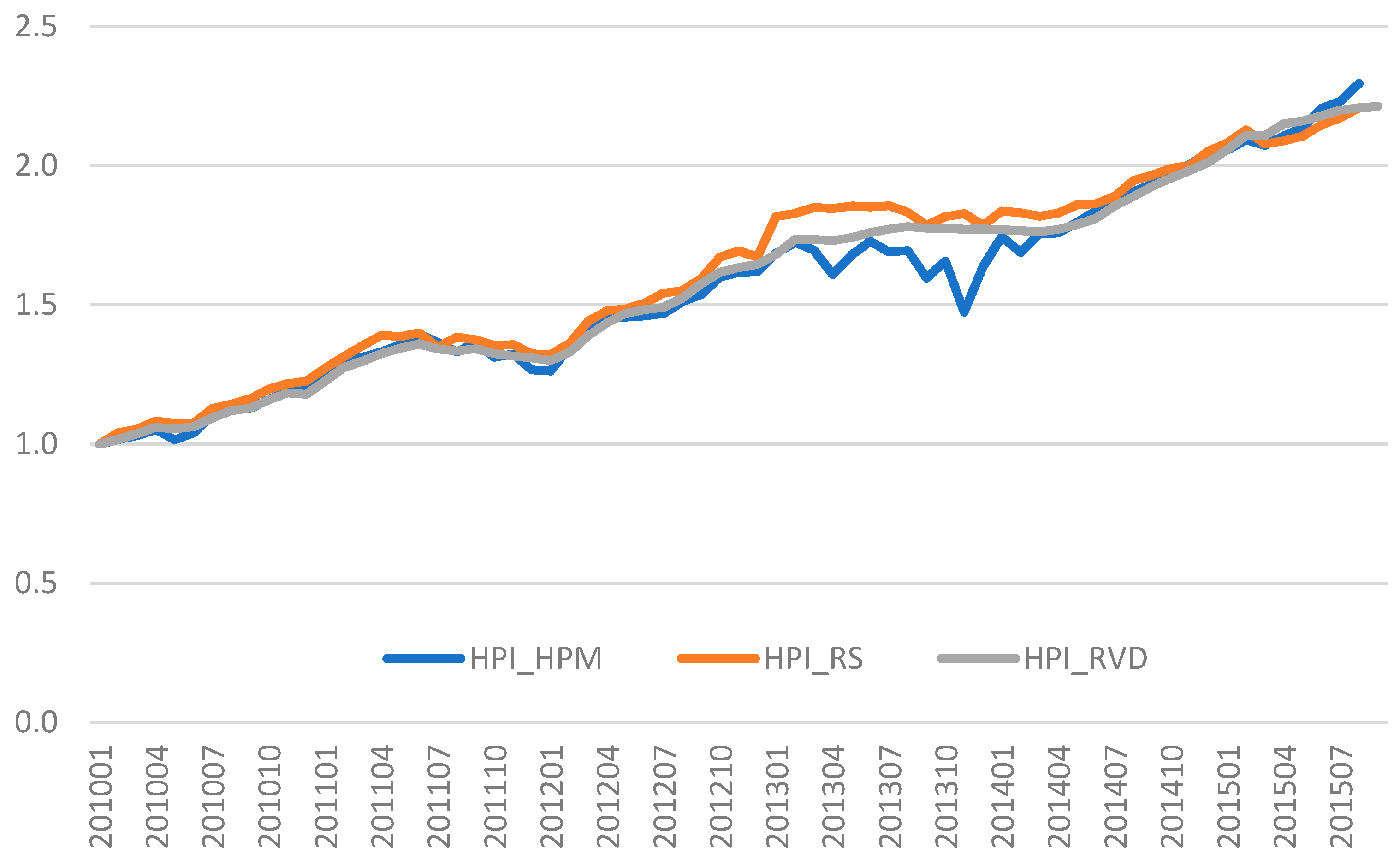
4.3. Repeat-Sales Method as a Robustness Check

One may argue that the premium or discount could be attributable to the specification error of the hedonic model. Therefore, the repeat-sales method is applied to serve as a robustness check. This method includes only the housing units with more than one transaction in the period. The repeat-sales method was initially proposed by Bailey et al. (1963) as a generalized procedure of the chained matched model applying to construct real estate price indices. The best-known repeat-sales indices are the Standard and Poors’ Case–Shiller Home Price Indices for 20 cities in the United States (OECD 2013). The method used the information on properties that were sold more than once. This matched-properties method does not require the control for period-to-period differences in the sample. More importantly, it prevents the estimation from specification errors and omitted variable bias. Endogeneity issues of buyers’ ethnicities, if any, could also be “differenced out” by the repeat-sales pairs as the initial buyer of a transaction, by definition, must be the sellers of the subsequent transaction in a repeat-sale. Like the hedonic model, to avoid any pre-sale effect on the price, we exclude all the transactions before completed construction in the sample. Thus, the number of observations reduces to 54,794, which, in comparison with international norms, is still a reasonably large sample for only six years. Table 4 shows the summary statistics of the repeat-sale pairs.
As mentioned in the literature review, previous studies were criticized for implicitly ignoring unobserved differences in housing quality within neighborhoods. We try to use the repeat-sales approach to provide an estimate with a clean identification. Equation (4) shows the repeat-sales model, which can be considered as the subtraction of Equation (2) of the first transaction from the second transaction of the same housing unit; hence differencing out all the structural and neighborhood quality variables, with the time dummy variables D j t redefined as follows.
l n ( P j t 2 / P j t 1 ) = β ( M L B t 2 M L S t 1 ) + t = 1 T α t D j t + ε j t    
l n ( P j t 2 / P j t 1 ) = β ( M L B t 2 M L S t 2 ) + t = 1 T α t D j t + ε j t    
Model (4) is a typical repeat-sales model incorporating a series of time dummy variables, D j t   with coefficients α t , where t ranges from period 0 to T (i.e., the period covered by the sample). For a particular pair of transactions, D j t takes the value −1 when t is the time of a previous sale of housing j, +1 when t is the time of the repeat-sale, and 0 when there are no sales of housing j at time t. It is worth noting that D j 0 was normalized to zero. Given the buyer in the first sale must be the seller in the second sale, so M L B t 1 in Equation (4) can be replaced by M L S t 2 , as shown in Equation (5).
Specifically, if ( M L B t 2 M L S t 2 ) = + 1 , it represents a non-local buyer engages with a local seller in the second sale; while if ( M L B t 2 M L S t 2 ) = 1 , it represents a local buyer engages with a non-local seller in the second sale, and 0 otherwise.11 To test for these two different effects, we fit the hedonic model that introduces separate terms for ( M L B t 2 M L S t 2 ) = + 1 and ( M L B t 2 M L S t 2 ) = 1 , such that:
l n ( P j t 2 / P j t 1 ) = β 3 ( M L B t 2 M L S t 2 ) + + β 4 ( M L B t 2 M L S t 2 ) + t = 1 T α t D j t + ε j t
where X+ is the second sale in which a non-local buyer engages with a local seller, 0 otherwise; and X is the second sale with a local buyer engaging with a non-local seller.
Table 5 reports the results of Equations (4)–(6). The results reinforce the findings for the hedonic price model in Equation (3) by identifying that non-local buyers/sellers are buying/selling at a price higher/lower from/to local buyers/sellers. The signs of the coefficients are consistent with that of Equation (3). The significance of the coefficient can be improved by converting from a monthly dummy to yearly dummy specifications (from Model (6) and (7)). The time effect estimated by both Equations (3) and (5) are plotted as the housing price indices in Figure 1.
They all track closely with the official government Rating and Valuation Department housing price index (HPI_RVD), except in 2013 because of the new stamp duties. One of the reasons for the mismatch in 2013 is Buyer’s Stamp Duty (BSD) imposition in October 2012 and the 1st Double Stamp Duty (DSD1) in February 2013. The BSD charges a flat rate of 15% for all non-local residents’ housing purchases, which sharply increases non-local buyers’ costs. The DSD1 charges a double rate of the then stamp duty for all non-first-time local buyers and non-local buyers, which reduces the number of transactions substantially, as shown in Figure 2.

5. A Critical Test for Information Asymmetry versus Anchoring Biases

Hitherto, the tests performed so far do not differentiate the hypotheses of information asymmetry from anchorage effects. As non-local buyers and sellers are likely to have higher search costs (i.e., asymmetric information), the non-local buyers’ premium or non-local sellers’ discount support the hypothesis of information asymmetry. Simultaneously, such premium/discount associated with the non-locals could be explained by the cognitive bias in which the non-locals rely heavily on market information in their city of origin (also known as the “anchor”) to make judgments in their purchase decisions. The “anchor” of price or rental yield is different from the locals (i.e., reference dependence).

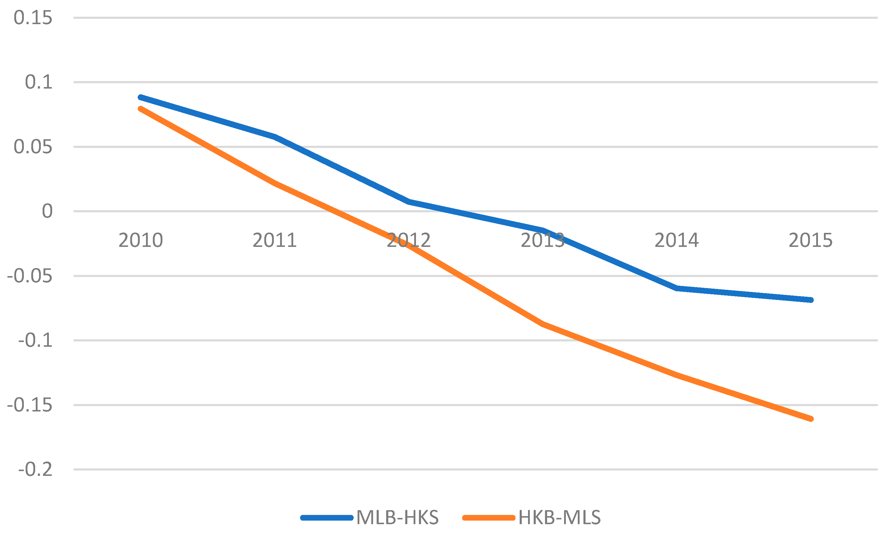
5.1. Difference-in-Differences Analysis and the Discussion on the Empirical Result

This study further uses a difference-in-differences approach to conduct a critical test to differentiate the information asymmetry from anchorage effects by exploiting the exogenous transaction taxes Buyer’s Stamp Duty (BSD) in October 2012 and the 1st Double Stamp Duty (DSD1) in February 2013 that applies to the non-locals’ home purchases. The transaction tax charges a flat rate of 15% BSD for all non-local residents’ housing purchases and charges a double rate of transaction tax for all non-locals (as well as non-first-time local buyers).
The hedonic price model, as stated in Equation (7), is performed. The equation incorporates two interactive terms of non-local sellers/buyers and time dummies. They measure the temporal changes of the discount/premium provided by the non-local sellers/buyers:
l n P i n t = α + β 1 M L B i + β 2 M L S i + s = 1 14 γ s S i s + n = 1 59 δ n N i n + t = 1 23 θ t T i t + t = 1 23 τ t b M L B i × T i t + t = 1 23 τ t s M L S i × T i t + ε i n t
where τ t b + β 1 ,   τ t s + β 2 measure any temporal changes of the premium and discount provided by non-local buyers and sellers relative to local ones. Given the model involves more variables in Equation (7), we convert the time dummies from 69 monthly to 23 quarterly variables to save some degree of freedom for ensuring their estimability. The results of model (7) are highly similar to model (3), except that the temporal changes of the price premium provided by non-local buyers ( t = 1 23 τ t b M L B i × T i t ) and the temporal changes of the price discount of non-local sellers ( t = 1 23 τ t s M L S i × T i t ) , i.e., the interaction terms are plotted in Figure 3.
As both transaction taxes are specific to non-local buyers (albeit the DSD further applies to all non-first-time homebuyers), these new transaction taxes would not impose any extra costs to non-local sellers compared to local sellers.12 Suppose the non-local price differential is attributable to asymmetric information. In that case, the non-local sellers’ price differentials should remain more or less unchanged after the new transaction tax, as their searching costs are still higher than local sellers. In contrast, if the anchorage bias hypothesis is dominant, then the extra transaction tax on buyers would make the market unappealing to both non-local buyers and sellers, as the new yield rate may become less than the anchored yield rate. For example, if the pre-tax yield rate is y, the anchored yield rate is Y, such that y > Y. After the transaction tax is imposed, the post-tax yield rate becomes 0.87y, given the non-local buyer pays 15% stamp duty more than the local counterparts. The new yield rate may no longer be greater than the anchored yield, resulting in a market-shifting effect. Such an effect would deter non-local buyers from buying and urge non-local sellers to sell.
Figure 3 confirms such de-anchoring effects. The temporal changes of the price differential of non-local buyers and sellers (i.e., the interaction terms of Equation (7)) indicate that before the new transaction tax imposed on non-locals, both non-local sellers and buyers had a price premium relative to locals, while after the tax, both non-local sellers and buyers gave a price discount. This result refutes the information asymmetry hypothesis and supports the hypothesis of anchorage effects because the yield rates of residential property investment in most tier-one cities in Mainland China were lower than that in Hong Kong. South China Morning Post (2017) reported that the rental yields in all the first-tier cities and the other nine second-tier cities in China were below 2%, in comparison with 4.7% in New York, 4.3% in Tokyo, and 2.4% in Hong Kong. However, after the extra 15% BSD on non-local buyers was charged with effect from October 2012, non-local sellers’ premium follows a downtrend. After a short period of adjustment, both non-local buyers and non-local sellers exhibited a significant housing price discount relative to the local buyers and sellers. The result further reinforces the hypothesis of anchorage bias that both non-local buyers and sellers would consider the new yield rate unattractive with reference to their anchored yield rates.
The divergence in their trading volumes further confirms the impacts on non-local buyers and sellers. Figure 4 shows the proportions of non-local to local buyers (MLB/HKB) and non-local to local sellers (MLS/HKS) in the period. The proportion of transactions of non-local sellers to local sellers was surging from an average of 3.5% to about 6.0% after the new stamp duties were imposed, reflecting the urge of non-local sellers to dispose of their properties compared with the local sellers. In contrast, the proportion of non-local buyers to local buyers fell to about 5% after the new stamp duties, mainly because of the unattractive rate of returns.

5.2. Difference-in-Differences Analysis and Discussion on the Results in the Repeat-Sales Setup

The difference-in-differences analysis is conducted in a repeat-sales model to generate more substantial evidence with the reversal of price differentials from a premium to a discount. The repeat-sales model further confirms the findings by including the temporal interaction terms, as shown in Equations (8) and (9). Figure 5 shows the results of the interaction terms of transactions engaged between non-local buyers and local sellers (MLS = 0, denoted by a + superscript) and that between local buyers and non-local sellers (MLB = 0, denoted by a − superscript).
l n ( P j t 2 / P j t 1 ) = β ( M L B t 2 M L S t 2 ) + t = 1 T τ t + D j t × ( M L B t 2 M L S t 2 ) + + t = 1 T α t D j t + ε j t
l n ( P j t 2 / P j t 1 ) = β ( M L B t 2 M L S t 2 ) + t = 1 T τ t D j t × ( M L B t 2 M L S t 2 ) + t = 1 T α t D j t + ε j t
The result is consistent with the hedonic pricing model. Both non-local buyers and sellers required a premium before the incidence of new non-local transaction tax, which refutes the asymmetric information hypothesis. After the new stamp duties are imposed explicitly on non-local buyers, the non-local buyers’ premium is reverted into a discount and the non-local sellers. The discount provided by non-local sellers (to local buyers) is even more than that of non-local buyers (obtained from local sellers). Additionally, our results of anchoring bias in the housing markets are in line with Scott and Lizieri’s (2012) results by an experimental approach, Bucchianeri and Minson’s (2013) results in house auctions, and Chang et al.’s (2016) result in out-of-state buyers.

6. Conclusions

The contribution of this paper is twofold. In terms of theoretical contribution, this is the first study to argue that other than a 4.9% non-local buyers’ premium, a 1.0% non-local sellers’ discount could simultaneously exist. There were very few empirical studies on the effects of transaction tax on non-local buyers with the same ethnicities, not to say, non-local sellers. Two alternative explanations for such price differentials of non-locals are considered, namely information asymmetry and anchoring effects. This study exploits an exogenous transaction tax targeted to non-locals in Hong Kong as a quasi-experiment to critically test the information asymmetry hypothesis against the anchorage effects. This specific transaction tax on non-locals allows us to identify the temporal changes of pricing strategies for non-local sellers and buyers by conducting a difference-in-differences analysis. The argument is that before introducing the transaction taxes, non-local Mainland buyers are more willing to pay a price premium due to their anchored low yield rates in China. Subsequent to the extra 15% BSD on non-local buyers were charged, such anchor of rental yield rates was distorted, and thus the price premium of non-locals vanished and exhibited even a discount. Indeed, the reversal of non-local price differential from premiums to discounts rules out the hypothesis of information asymmetry because the search cost of non-local sellers, if any, should be time-invariant and not be influenced by transaction taxes. The difference-in-differences results in both the hedonic price and repeat-sales models refute the asymmetric information hypothesis and incline to confirm the prevalence of anchorage effects.
In terms of empirical contribution, this study develops a novel machine learning algorithm with natural language processing to identify the non-local Mainland Chinese from the local Hong Kong Chinese in a residential property transaction database based on the romanization feature of Chinese names. This approach of identifying non-local buyers and sellers provides another advantage in controlling unobservable differences due to cultural and ethnic differences. The reversal of non-local price differential from premiums to discounts in our empirical test also implies that the selected machine learning algorithm can successfully identify the non-locals who are the only buyers paying the foreign buyer taxes. Indeed, machine learning algorithms are relatively new in real estate research. So far, most applications are merely focusing on mass appraisals or improving specific predictive analytics. To the best of our knowledge, using a machine-learning approach, along with hedonic and repeat sales methods to test anchoring and asymmetric information theories in the real estate market is new, if not novel, in terms of methodology.
One important application of machine learning is to directly test theories that are inherently about predictability. For empirical researchers, theory and data-driven analysis have always coexisted. While many estimations are based on top-down, theory-driven, and deductive reasoning, machine learning adopted a bottom-up, data-driven, and inductive reasoning approach to let the data speak themselves more clearly than ever. In fact, these two approaches need not be in conflict (Mullainathan and Spiess 2017). This study aims to serve as a convincing demonstration as such. Search theory and behavioral economics guide us to what variables to manipulate in a quasi-experiment; in analyzing the data, machine learning could help manage multiple outcomes and estimate heterogeneous treatment effects. This real estate study presents a new way of using machine learning that gives its place in the econometric toolkit. It is imperative to know that machine learning provides new tools that eventually increase research scope and solve more new challenging problems. To facilitate researchers applying our developed algorithm on their projects, the source code and a user manual are uploaded to Github. We believe that these findings and machine-learning applications will substantially impact academic research by opening up new research directions to critically test alternative hypotheses, which embraces Platt’s (1964) strong inference of scientific thinking.

Author Contributions

Conceptualization, K.S.C., J.T.C. and S.L.; methodology, K.S.C., J.T.C. and C.Y.Y.; software, K.S.C. and J.T.C.; validation, K.S.C. and C.Y.Y.; formal analysis, K.S.C., J.T.C., S.L. and C.Y.Y.; data curation, K.S.C., J.T.C. and S.L.; writing—original draft preparation, K.S.C., J.T.C. and S.L.; writing—review and editing, K.S.C. and C.Y.Y.; visualization, K.S.C. and C.Y.Y.; supervision, K.S.C.; project administration, K.S.C. All authors have read and agreed to the published version of the manuscript.

Funding

This research received no external funding.

Institutional Review Board Statement

Not applicable.

Informed Consent Statement

Not applicable.

Data Availability Statement

Restrictions apply to the availability of these 3rd party data. Data were obtained from the Economic Property Research Centre (EPRC) in Hong Kong and are available by subscribing to EPRC at http://eprc.com.hk/index.htm (accessed on 30 August 2021).

Conflicts of Interest

The authors declare no conflict of interest. The views expressed here are solely the authors’ and do not represent the views of Bates White, Freddie Mac, or their other employees. All errors are our own.

Appendix A

A Simple Model to Develop Hypotheses
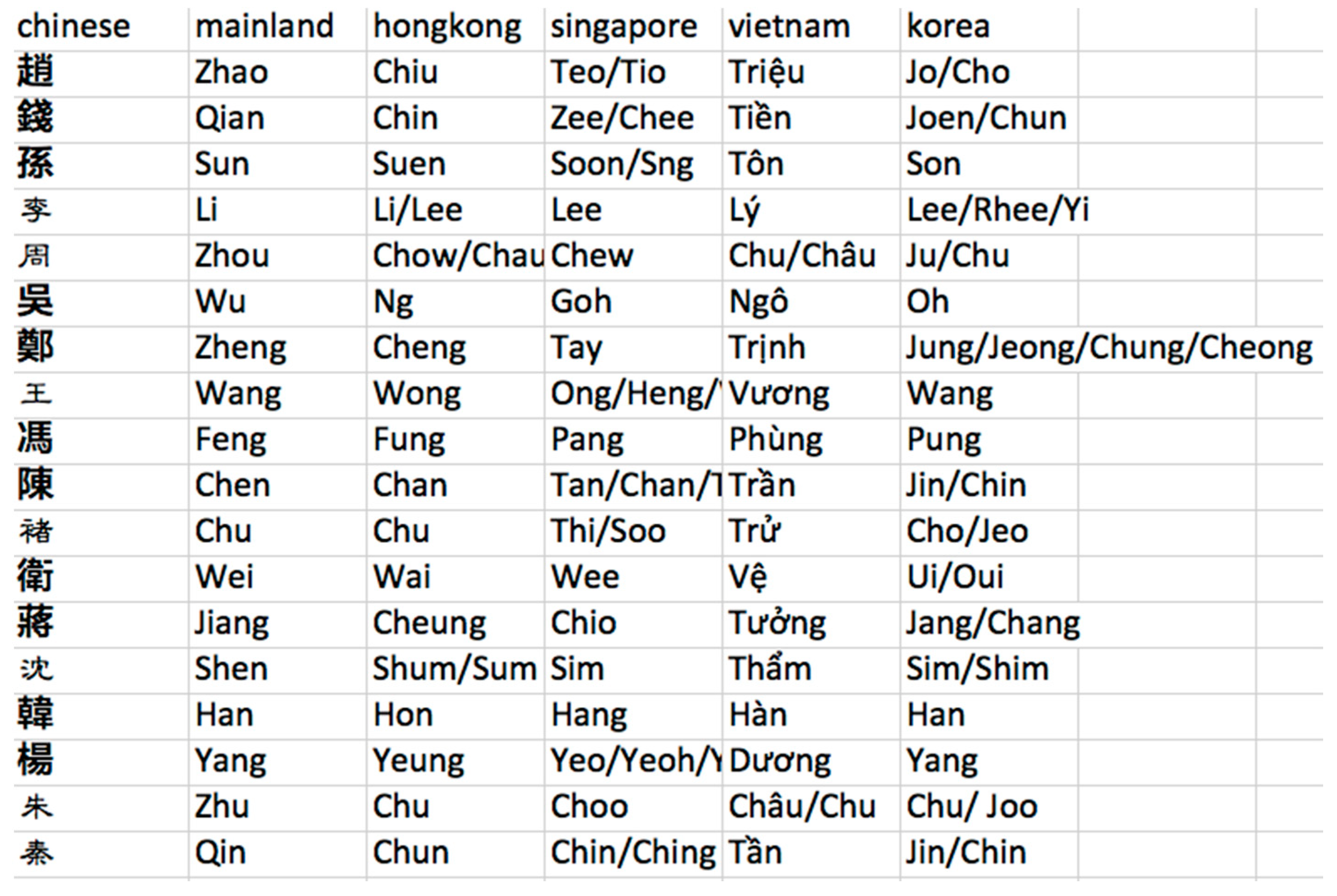
Consider a sequential search model for heterogeneous buyers of real estate (Lambson et al. 2004). Assume that apartment owners are willing to sell at different prices p, where F() is the distribution of per-unit prices. F(p) is the probability the buyer finds an offer to sell at p ∈ (0, ∞) in an independent offer. In this simple search model, the total cost of purchasing apartment units consists of the price paid for the apartments plus the costs incurred to discover the price.
Buyers search on the market with different beliefs about price distribution. Specifically, buyers perceive that the distribution of per-unit prices is F(p, b), where b ∈ (−∞, ∞) is a parameter that shifts some of the probability weight. In each round, a buyer needs to pay a fixed marginal search cost, c ∈ (0, ∞), to obtain an offer in which an owner is willing to sell a unit of real space at a per-unit price p. Thus, the price for a piece of real estate is ap. The buyer then chooses to agree to the seller’s asking price (i.e., accepting an offer) or to continue to search (i.e., rejecting the offer). Having already paid the (sunk) search cost, the net value or surplus from buying at price p is a(vp), where v ∈ (0, ∞) is the value per unit (i.e., the present value of cash flows for each property) calculated by the buyer.
Under the unconstrained search horizon, for the reservation price to be optimal, buyers will continue to search until the marginal cost of searching equals the expected marginal benefit, where
c = 0 p * a ( p * p ) f ( p , b ) d p
Since p∗ is a function of the primitive variables, implicit differentiation with respect to a, c, and b results in three comparative statics, namely p * / a < 0 , p * / c > 0 , and p * / b > 0   .13 The first focus of our paper is on the asymmetric information hypothesis (H1), which is stated by the implicit differentiation results of p * with respect to c, i.e., p * / c > 0 . Intuitively, ceteris paribus, the higher the search cost the non-local buyers incur, the higher reservation prices they have, and the sooner they stop searching and pay higher prices than their low-search-cost local counterparts. However, many buyers are constrained by time. When buyers have constrained search horizons (i.e., they intend to anchor on certain beliefs), where T is the maximum number of searches allowed, the optimal strategy is to set a sequence of reservation prices ( p 1 * ,   ,   p T * ) , which aligns with (or anchors) one’s values, beliefs, and prior knowledge. Thus, after c was paid, the value of having found the price per unit p t in round t is:
W t ( p t ) = m a x { a ( v     p t ) , 0 W t + 1 ( p ) f   ( p ,   b ) d p     c }
Compared to a buyer with one extra round to search, the price at round t, ( p t ) , will have the same sequence of (believed) reservation prices as the buyer at t − 1, ( p t 1 * ) plus one additional draw at the beginning with reservation price. A backward induction implies that reservation prices are increasing at time t, i.e., p t * > p t 1 * , for all t. That extra price will lead buyers with longer horizons to pay less, on average, than buyers with shorter horizons, which means E T + 1 ( p ) E T ( p ) . This implies that the greater the search horizon, the lower the expected per unit price.
There are two testable hypotheses here. As the search model shows that a non-local price premium (relative to the locals) is possible if non-local buyers (i) are more time-constrained (T), (ii) have higher search costs (c) and/or (iii) believe that the distribution of prices F(p, b) is higher than that for local buyers. The belief that the non-locals anchor on their belief in a set of reservation prices and conduct less searching illustrates that a non-local price premium is possible. That provides us with a basis to test our hypotheses of anchoring biases (H2), which states: ceteris paribus, non-local buyers who are more time-constrained and who believe that the distribution of prices F(p, b) is higher than local buyers believe, the higher reservation prices they have compared to their less time-constrained local counterparts. Thus, non-local price premium results.
In the empirical tests, we will use the housing market in Hong Kong as a case study to show that non-local buyers and sellers pay price premiums in the real estate market. Other than just testing the anchoring biases premium, we further argue that as non-locals are anchoring on a very different perspective on asset returns from that of locals, they may believe that reservation prices may be low enough for a price discount. More importantly, we exploit an exogenous policy change in transaction tax on non-local buyers in 2013 as an intervention, and the corresponding locals as counterfactuals, to confirm that such non-local price premium (or discount in this case) is due to the effect of anchoring biases.

Appendix B

An Analysis of Naming Patterns among Mainland Chinese
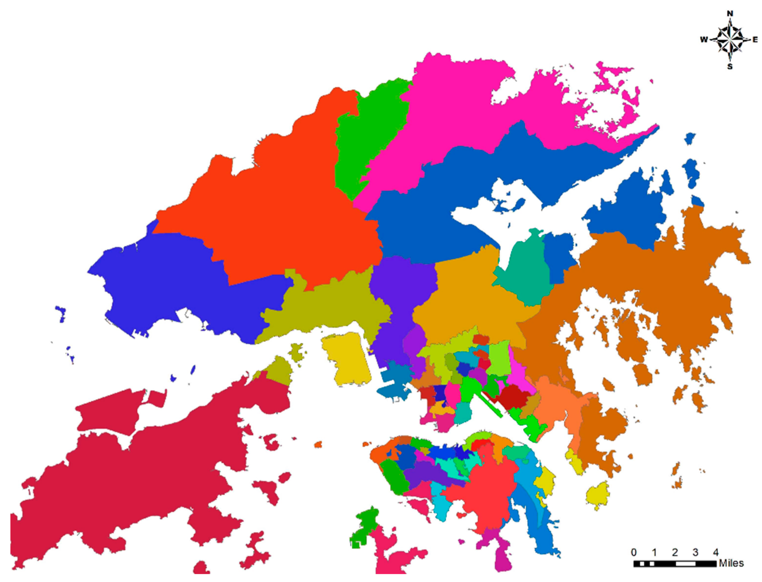
The Romanized names of Chinese are distinct across different regions. Due to the history of the former colony, Hong Kong and Mainland China adopt different romanization of Chinese people’s names. It is relatively straightforward to tell whether a person was born in Mainland China or Hong Kong by referring to their Romanized names in English. Cantonese and English are the most widely used languages in Hong Kong, while Mandarin is Mainland China’s official language. Chinese uses a logographic script, and its characters do not represent phonemes directly. The “romanization” of Chinese refers to the use of the Latin alphabet to write Chinese.
There have been many systems using Roman characters to represent the Chinese throughout history. However, since 1982 Hanyu Pinyin has become an international standard. The Hong Kong Government has been adopting the Eitel/Dyer-Ball system of romanization based on the spoken Cantonese language. It was first adopted in 1960 to standardize the romanization of place-names throughout Hong Kong (Hong Kong, Kowloon, and New Territories). Since then, this romanization system has been extended to local Hong Kong citizens’ Chinese names, which gives Romanized Hong Kong Chinese names a distinctive character different from that in Mainland China. The romanization of common Chinese surnames is illustrated in Figure A1. This difference in the romanization of Chinese names allows us to carry out a large-scale empirical test on the hypothesized premium (discount) paid by non-local buyers (sellers).
Figure A1. Examples of Common Chinese Surnames and their Romanization of various ethnicities. Notes: Romanization is the conversion of writing from a different writing system to the Roman (Latin) script. Despite the same written form of Chinese, the romanization is different in Mainland China (Mandarin), Hong Kong (Cantonese), Singapore (Singaporean), Vietnam (Vietnamese) and Korea (Korean).
Jrfm 14 00423 g0a1

Appendix C

Figure A2. Hong Kong 52 Housing subdistricts categorized by Economic Property Research Centre (EPRC). Data Source: EPRC; Retrieved from the interactive map at http://www.eprc.com.hk/DistrictBoundary/ (accessed on 30 August 2021).
Jrfm 14 00423 g0a2

Note

1.
To test the effects of government policies on non-local buyers and sellers, we limit our sample period from 2010 to 2015. The special tax for non-local buyers (Buyers’ Stamp Duty) was implemented in October 2012, but the 2nd Double Stamp Duty of a uniform 15% rate applied on both local and non-local buyers did not apply till November 2016. Better still, the period can exclude the effect of the first and only development of sale restrictions on non-native buyers, One Kai Tak, as it was not open for sale until August 2016.
2.
The statistics from the government audit’s report, Director of Audit’s Report No. 66: Chapter 4—Admission Schemes for Talent, Investors and Workers, Annex D: Statistics on entrants having acquired Hong Kong permanent resident status under various immigration policies/admission schemes, and having stayed in Hong Kong for seven years or more; retrieved from https://www.legco.gov.hk/yr15-16/english/pac/reports/66/app_13.pdf (accessed on 30 August 2021) indicate that the number of entrants who have acquired Hong Kong permanent resident status under various immigration policies remains low, fewer than 8000 per year.
3.
Local movers are assumed to have their own uniform level of search costs.
4.
The source code and model are publicly available at Github.
5.
The examples could be from an external source.
6.
Researchers can verify the accuracy using a hold-out sample known as testing data. We will discuss our procedure in this section.
7.
Others include non-Hong Kong or mainland Chinese names and company names.
8.
Dilution or dropout is a regularization technique that randomly omitting weights in a neural network model.
9.
We acknowledge that there could be limitations to our method of identifying non-local sellers and buyers. First, many investors from Mainland China would buy housing units in Hong Kong via buying companies, and the pricing information of these company transactions is not reflected from normal housing transaction data. Second, some Chinese with Mainland Chinese’s last names may have lived in Hong Kong for some years and may be as experienced as local participants, but their number is small. However, the reversal of non-local price differential from premiums to discounts in our empirical findings implies that our machine-learning algorithm can successfully identify the non-locals given they are the only buyers who have to pay the foreign buyers’ stamp duties.
10.
On 4 November 2016, the Hong Kong Government amended the Stamp Duty Ordinance to increase the ad valorem stamp duty rates for all residential property transactions to a flat rate of 15 percent, with immediate effect. It is considered “a significant leap from the so-called [1st] “Double Stamp Duty” under the current regime, which stands at a range of 4.25 to 8.5 percent, being applicable to purchases by non-Hong Kong permanent residents and/or if the purchaser already owns another residential property at the time of the subsequent purchase.” (Yip 2016).
11.
Equation (4) shows the typical repeat-sale model which subtracts the first-sale equation from the second-sale equation. Following the Hedonic Price Model (Equation (2)), we do not use Equation (3) is because most of the repeat-sales samples involve only one pair of repeat-sales in the study period, which does not provide information of the name of the seller in the first sale.
12.
Even if the sellers are to share part of the new stamp duties under the market negotiation process, the average market sharing ratio should be the same for both the local and non-local sellers.
13.
The three comparative statics are p * a = 0 p * ( p * p ) f   ( p ,   b )   d p   F ( p * ,   b ) < 0 ;   p * c = 1 a F ( p * ,   b ) > 0 ;   p * a = 0 p * ( p * p ) f b   ( p ,   b )   d p   a F ( p * ,   b ) > 0 .

References

  1. Akerlof, George A. 1970. The Market for “Lemons”: Quality Uncertainty and the Market Mechanism. The Quarterly Journal of Economics 84: 488–500. [Google Scholar] [CrossRef]
  2. Bailey, Martin J., Richard F. Muth, and Hugh O. Nourse. 1963. A Regression Model for Real Estate Price Index Construction. Journal of the American Statistical Association 58: 933–42. [Google Scholar] [CrossRef]
  3. Bucchianeri, Grace W., and Julia A. Minson. 2013. A homeowner’s dilemma: Anchoring in residential real estate transactions. Journal of Economic Behavior & Organization 89: 76–92. [Google Scholar] [CrossRef]
  4. Camerer, Colin F., and George Loewenstein. 2003. Behavioral economics: Past, present, future. In Advances in Behavioral Economics. Princeton: Princeton University Press. [Google Scholar]
  5. Chang, Chuang-Chang, Ching-Hsiang Chao, and Jin-Huei Yeh. 2016. The role of buy-side anchoring bias: Evidence from the real estate market. Pacific-Basin Finance Journal 38: 34–54. [Google Scholar] [CrossRef]
  6. Cho, Kyunghyun, Bart Van Merriënboer, Caglar Gulcehre, Dzmitry Bahdanau, Fethi Bougares, Holger Schwenk, and Yoshua Bengio. 2014. Learning phrase representations using RNN encoder-decoder for statistical machine translation. arXiv arXiv:1406.1078. [Google Scholar]
  7. Clauretie, Terrence M., and Paul D. Thistle. 2007. The Effect of Time-on-Market and Location on Search Costs and Anchoring: The Case of Single-Family Properties. The Journal of Real Estate Finance and Economics 35: 181–96. [Google Scholar] [CrossRef]
  8. Diaz, Julian, III, and Marvin L. Wolverton. 1998. A Longitudinal Examination of the Appraisal Smoothing Hypothesis. Real Estate Economics 26: 349–58. [Google Scholar] [CrossRef]
  9. Edelstein, Robert, and Wenlan Qian. 2014. Short-Term Buyers and Housing Market Dynamics. The Journal of Real Estate Finance and Economics 49: 654–89. [Google Scholar] [CrossRef] [Green Version]
  10. Elder, Harold W., Leonard V. Zumpano, and Edward A. Baryla. 1999. Buyer Search Intensity and the Role of the Residential Real Estate Broker. The Journal of Real Estate Finance and Economics 18: 351–68. [Google Scholar] [CrossRef]
  11. Garmaise, Mark J., and Tobias J. Moskowitz. 2004. Confronting information asymmetries: Evidence from real estate markets. The Review of Financial Studies 17: 405–37. [Google Scholar] [CrossRef]
  12. Haley, Alex. 1983. Ethnic Genealogy: A Research Guide. Santa Barbara: ABC-CLIO. [Google Scholar]
  13. Harding, John P., John R. Knight, and C. F. Sirmans. 2003a. Estimating bargaining effects in hedonic models: Evidence from the housing market. Real Estate Economics 31: 601–22. [Google Scholar] [CrossRef]
  14. Harding, John P., John R. Knight, and C. F. Sirmans. 2003b. Estimating bargaining power in the market for existing homes. The Review of Economics and Statistics 85: 178–88. [Google Scholar] [CrossRef]
  15. Humphreys, Brad R., Adam Nowak, and Yang Zhou. 2019. Superstition and real estate prices: Transaction-level evidence from the US housing market. Applied Economics 51: 2818–41. [Google Scholar] [CrossRef]
  16. Ihlanfeldt, Keith, and Tom Mayock. 2009. Price Discrimination in the Housing Market. Journal of Urban Economics 66: 125–40. [Google Scholar] [CrossRef]
  17. Ihlanfeldt, Keith, and Tom Mayock. 2012. Information, Search, and House Prices: Revisited. Journal of Real Estate Finance and Economics 44: 90–115. [Google Scholar] [CrossRef]
  18. Lambson, Val E., Grant R. McQueen, and Barrett A. Slade. 2004. Do Out-of-State Buyers Pay More for Real Estate? An Examination of Anchoring-Indexed Bias and Search Costs. Real Estate Economics 32: 85–126. [Google Scholar] [CrossRef]
  19. Lichtenstein, Sarah, and Paul Slovic. 1971. Reversal of Preferences between Bids and Choices in Gambling Decisions. Journal of Experimental Psychology 89: 46–55. [Google Scholar] [CrossRef] [Green Version]
  20. Ling, David C., Andy Naranjo, and Milena T. Petrova. 2018. Search Costs, Behavioral Biases, and Information Intermediary Effects. The Journal of Real Estate Finance and Economics 57: 114–51. [Google Scholar] [CrossRef]
  21. Liu, Yu, Paul Gallimore, and Jonathan A. Wiley. 2015. Non-local investors: Anchored by their markets and impaired by their distance. The Journal of Real Estate Finance and Economics 50: 129–49. [Google Scholar] [CrossRef]
  22. Mikolov, Tomas, Kai Chen, Greg Corrado, and Jeffrey Dean. 2013. Efficient estimation of word representations in vector space. arXiv arXiv:1301.3781. [Google Scholar]
  23. Mullainathan, Sendhil, and Jann Spiess. 2017. Machine learning: An applied econometric approach. Journal of Economic Perspectives 31: 87–106. [Google Scholar] [CrossRef] [Green Version]
  24. Neo, Poh Har, Seow Eng Ong, and Yong Tu. 2008. Buyer exuberance and price premium. Urban Studies 45: 331–45. [Google Scholar]
  25. Northcraft, Gregory B., and Margaret A. Neale. 1987. Expert, Amateurs, and Real Estate: An Anchoring-and-Adjustment Perspective on Property Pricing Decisions. Organizational Behavior and Human Decision Processes 39: 84–97. [Google Scholar] [CrossRef]
  26. OECD. 2013. Repeat Sales Methods. In Handbook on Residential Property Price Indices. Luxembourg: Eurostat, chp. 6. [Google Scholar] [CrossRef]
  27. Pace, R. Kelley, and Darren Hayunga. 2020. Examining the Information Content of Residuals from Hedonic and Spatial Models Using Trees and Forests. The Journal of Real Estate Finance and Economics 60: 170–80. [Google Scholar] [CrossRef]
  28. Platt, John R. 1964. Strong Inference. Science 146: 347–53. [Google Scholar] [CrossRef] [PubMed] [Green Version]
  29. Rosen, Sherwin. 1974. Hedonic prices and implicit markets: Product differentiation in pure competition. Journal of Political Economy 82: 34–55. [Google Scholar] [CrossRef]
  30. Salehinejad, Hojjat, Sharan Sankar, Joseph Barfett, Errol Colak, and Shahrokh Valaee. 2017. Recent advances in recurrent neural networks. arXiv arXiv:1801.01078. [Google Scholar]
  31. Scott, Peter J., and Colin Lizieri. 2012. Consumer house price judgements: New evidence of anchoring and arbitrary coherence. Journal of Property Research 29: 49–68. [Google Scholar] [CrossRef]
  32. Shen, Lily, and Stephen Ross. 2021. Information value of property description: A machine learning approach. Journal of Urban Economics 121: 103299. [Google Scholar] [CrossRef]
  33. South China Morning Post. 2017. Plunging Chinese Rental Yields Point to Property Bubbles in Major Cities. South China Morning Post. July 18. Available online: https://www.scmp.com/business/china-business/article/2103116/plunging-chinese-rental-yields-point-property-bubbles-major (accessed on 30 August 2021).
  34. Sun, Hua, and Seow Eng Ong. 2014. Bidding Heterogeneity, Signaling Effect and its Implications on House Seller’s Pricing Strategy. The Journal of Real Estate Finance and Economics 49: 568–97. [Google Scholar] [CrossRef]
  35. Turnbull, Geoffrey K., and Casey F. Sirmans. 1993. Information, Search, and House Prices. Regional Science and Urban Economics 23: 545–57. [Google Scholar] [CrossRef]
  36. Watkins, Craig. 1998. Are New Entrants to the Residential Property Market Informationally Disadvantaged? Journal of Property Research 15: 57–70. [Google Scholar] [CrossRef]
  37. Wong, Kai On, Osmar R. Zaïane, Faith G. Davis, and Yutaka Yasui. 2020. A machine learning approach to predict ethnicity using personal name and census location in Canada. PLoS ONE 15: e0241239. [Google Scholar] [CrossRef] [PubMed]
  38. Wright, Danika, and María B. Yanotti. 2019. Home advantage: The preference for local residential real estate investment. Pacific-Basin Finance Journal 57: 101167. [Google Scholar] [CrossRef] [Green Version]
  39. Yip, Alan. 2016. HK Residential Property Stamp Duty Jump to 15%. Industry Insights, Hong Kong Lawyer, December. Available online: http://www.hk-lawyer.org/content/hk-residential-property-stamp-duty-jump-15 (accessed on 30 August 2021).
  40. Yiu, Chung Yim. 2009. Disentanglement of Age, Time, and Vintage Effects on Housing Price by Forward Contracts. Journal of Real Estate Literature 17: 273–91. [Google Scholar] [CrossRef]
  41. Zhou, Xiaorong, Karen Gibler, and Velma Zahirovic-Herbert. 2015. Asymmetric Buyer Information Influence on Price in a Homogenous Housing Market. Urban Studies 52: 891–905. [Google Scholar] [CrossRef]
  42. Zumpano, Leonard V., Harold W. Elder, and Edward A. Baryla. 1996. Buying a house and the decision to use a real estate broker. The Journal of Real Estate Finance and Economics 13: 169–81. [Google Scholar] [CrossRef]
Figure 1. Estimated Housing Price Indices, 2010M1–2015M9. Notes: HPI_DVD is the housing price index compiled by the Rating and Valuation Department of Hong Kong (HPI_RVD). Housing Price Indices estimated by the Hedonic Price Model in Equation (3) (HPI_HPM) and repeat-sales model (HPI_RS) in Equation (5) are shown to compare the official government housing price index.
Jrfm 14 00423 g001
Figure 2. Transactions of Residential Properties in Hong Kong, 2010M1–2015M9. Notes: the number of transactions of residential properties in Hong Kong drops after the introduction of the Seller’s Stamp Duty (SSD) in November 2010, the Buyer’s Stamp Duty (BSD) in October 2012, and the 1st Double Stamp Duty (DSD1) in February 2013.
Jrfm 14 00423 g002
Figure 3. Temporal Changes of Price Differentials for Non-local Buyers and Sellers. Notes: The chart illustrates the coefficients estimated by Model (3) of the interactive terms between time and non-local buyers MLB ( τ t b + β 1 ) as well as the interactive terms between time and non-local sellers MLS ( τ t s + β 2 ) . The results vividly indicate that non-local price premia are changed into a non-local discount after the non-local specific stamp duties are introduced in circa 2012/13.
Jrfm 14 00423 g003
Figure 4. Proportions of Transactions of Non-local to Local Buyers and Sellers. Notes: the proportion of transactions of non-local buyers to local buyers (MLB/HKB)—left axis, the proportion of transactions of non-local sellers to local sellers (MLS/HKS)—right axis.
Jrfm 14 00423 g004
Figure 5. Temporal Changes of Price Differentials for Non-local Buyers and Sellers in Repeat-sale Model. Notes: MLB-HKS represents the coefficients of the interactive terms denoted by τ t + + β in the Equation (8) that non-local buyers engage with the local seller (i.e., MLS = 0), HKB-MLS represents the coefficients of the interactive terms denoted by τ t β in Equation (9) that local buyers engage with the non-local seller (i.e., MLB = 0). The time dummies are yearly dummies.
Jrfm 14 00423 g005
Table 1. Structure, hyperparameters and performance of the model.
Panel A—Hyperparameters of the Machine Learning Model
SequenceLayerHyperparameterValue
1st layerWord EmbeddingMax length50
Number of embeddings30
2nd layerGRUNumber of layers3
Number of neurons30
3rd layerActivationFunctional formtanh
4th layerDropoutProbability of dropout20%
5th layerMLPNumber of layers2
Number of neurons10
ActivationSigmoid
Panel B—Performance of the Machine Learning Model
Training SampleValidation SampleTesting Sample
99.14%98.94%99.00%
Table 2. Summary statistics of variables for the hedonic price model.
VariableDescriptionMean/
Count
S.D.Min.Max.
PSales Price (in HK$ Million)4.013.570.10236
AGEBuilding Age (in years)20.4010.40−3.2558
FLRFloor Level (in Storey)16.9512.150.0086
GFAGross Floor Area (in sq ft)655.49242.21346315
U_RATIOUtility Ratio = Saleable to Gross Floor Area (in sq ft)0.780.060.320.99
BWBay Window Area (in sq ft)15.3115.730.00250
LEASERemaining land lease period
(in years)
111.47223.5512890
PRESALEPre-sale Dummies238-01
MLSMainland Seller (1, or 0 otherwise)5265-01
MLBMainland Buyer (1, or 0 otherwise)7632-01
Direction Dummies8
Time Dummies692010M1–2015M9
District Dummies59Appendix C
Source: Economic Property Research Centre (EPRC). Notes: The 59 district dummy variables are illustrated in Appendix C. The time dummies are 69 monthly time dummies from January 2010 to September 2015. The direction dummies include the east (D_E), west (D_W), south (D_S), north (D_N), north-east (D_NE), north-west (D_NW), south-east (D_SE), and south-west (D_SW). To avoid exact collinearity, one neighborhood dummy, the first period time dummy (January 2010), and the direction east (D_E) are omitted as the base case. Mainland sellers and buyers are identified by using the machine learning algorithm outlined in another section.
Table 3. The results of the hedonic price model.
Equation (1) BaselineEquation (2)Equation (3)
Dep. Var.The Logarithm of Sales Prices ln(P)
MLB-0.0490.049
(0.003) ***(0.003) ***
MLS--−0.010
(0.004) ***
|AGE| × PRESALE0.135−0.128−0.124
(0.100)(0.100)(0.100)
AGE × (1 − PRESALE)−0.012−0.012−0.012
(0.000) ***(0.000) ***(0.000) ***
FLR0.0030.0030.003
(0.000) ***(0.000) ***(0.000) ***
GFA0.0010.0010.001
(0.000) ***(0.000) ***(0.000) ***
U_RATIO1.6801.6811.681
(0.020) ***(0.020) ***(0.020) ***
BW0.0030.0030.003
(0.000) ***(0.000) ***(0.000) ***
LEASE0.0000.0000.000
(0.000) ***(0.000) ***(0.000) ***
Constant−0.862−0.865−0.865
(0.016) ***(0.016) ***(0.016) ***
Direction Fixed EffectIncluded (8 Directions)
Time Fixed EffectIncluded (2010M1–2015M9)
Neighbourhood Fixed EffectIncluded (59 Subdistricts)
Observations:93,72693,72693,726
R-squared:0.8510.8520.852
Notes: The dependent variable ln(P) is the logarithm of the transacted house prices in Hong Kong dollars, and *, **, *** mean that the coefficient is significant at the 10%, 5%, 1% levels. Figures in the parentheses are the standard errors.
Table 4. Summary statistics of variables for the repeat-sales model.
DescriptionMean/
Count
S.D.MinMax
P1Price of the first sale in a repeat-sale2.933.360.10344.88
P2Price of the second sale in a repeat-sale3.893.830.10528.80
MLBMainland Buyer (1, or 0 otherwise)2860
MLSMainland Seller (1, or 0 otherwise)2895
Notes: Only the numbers of counts are shown for dummy variables.
Table 5. Results of the repeat-sales models of Equations (4)–(6).
Dep. Var: ln ( P j t 2 / P j t 1 )
VariableModel (4)Model (5)Model (6)
M L B t 2 M L S t 1 0.0283
(0.0037) ***
( M L B t 2 M L S t 1 ) + 0.0067
(0.0053)
0.0025
(0.0055) ***
( M L B t 2 M L S t 1 ) −0.0499
(0.0053) ***
−0.0381
(0.0055) ***
Time Fixed EffectsYes (2010M1–2015M9)Yes (2010–2015)
Observations54,79454,79454,794
R-squared0.22880.23020.1741
Notes: The dependent variable ln(P) is the logarithm of the transacted house prices in Hong Kong dollars, and *** mean that the coefficient is significant at 1% level. Figures in the parentheses are the standard errors.
Publisher’s Note: MDPI stays neutral with regard to jurisdictional claims in published maps and institutional affiliations.

