
The Optimal Spending Rate versus the Expected Real Return of a Sovereign Wealth Fund
Department of Business and Management Science, Norwegian School of Economics, 5045 Bergen, Norway
*
Authors to whom correspondence should be addressed.
J. Risk Financial Manag. 2021, 14(9), 425; https://0-doi-org.brum.beds.ac.uk/10.3390/jrfm14090425
Submission received: 24 June 2021
/
Revised: 19 July 2021
/
Accepted: 22 July 2021
/
Published: 6 September 2021
(This article belongs to the Section Mathematics and Finance)
Abstract
:We consider a sovereign wealth fund that invests broadly in the international financial markets. The influx to the fund has stopped. We adopt the life cycle model and demonstrate that the optimal spending rate from the fund is significantly less than the fund’s expected real rate of return. The optimal spending rate ensures that the fund will last “forever”. Spending the expected return will deplete the fund with probability one. Moreover, this strategy is inconsistent with optimal portfolio choice. Our results are contrary to the idea that it is sustainable to spend the expected return of a sovereign wealth fund.
Keywords:
optimal spending rate; endowment funds; expected utility; risk aversion; EIS; recursive utilityJEL Classification:
G10; G12; D9; D51; D53; D90; E211. Introduction
We consider optimal investment strategies and the associated optimal extraction from an endowment fund consistent with the life cycle model. We demonstrate that the optimal spending rate is strictly smaller than the expected rate of return. The difference is far from negligible, and amounts to several percentage points in most real situations.
The basic explanation is: If the fund is managed by diversification, this means that risk aversion, consumption substitution and impatience are essential in the optimal portfolio choice problem. Then, to be consistent, the spending rate must also reflect this. Accordingly, the expected real rate of return is typically not an optimal spending rate, since this criterion would normally be associated with risk neutrality.
We take the security market as given—it is assumed to be in equilibrium—and introduce a price taking agent in this market. In this setting we reconsider the problem of optimal consumption and portfolio selection. In the context of an endowment fund, the results from analyzing this more general problem can immediately be utilized in order to determine an optimal spending rate. We have considered both expected utility, in which case risk aversion plays a prominent role, and recursive utility, in which case consumption substitution is separated from risk aversion and is also important.
When the investment opportunity set is deterministic, there exist explicit and closed-form solutions for optimal extraction. Rather than depending upon the expected rate of return, the optimal extraction rate is a convex combination of the impatience rate and the certainty equivalent rate of return. The latter quantity is significantly smaller than the expected rate of return. This is normally true also for the impatience rate, and thus for the convex combination.
For a stochastic investment opportunity set, we present formulas herein which we believe are original. First and foremost, these solutions are demonstrated to result in smaller values than the expected real rate of return on the endowment fund, for plausible values of the preference parameters and the other parameters of the problem. The difference is significant in most cases.
If the extraction rate is the one of expected return, this normally means that the agent is risk neutral at the level of spending, and must then, to be consistent, be risk neutral at the level of optimal portfolio selection as well. However, the consequence of such an investment strategy is rarely advocated by anyone responsible for an endowment fund, whatever its purpose.
We demonstrate that a popular and much advertised extraction policy, the expected real rate, is not consistent with a sustainable spending rate, and will with probability one eventually deplete any fund that is managed by diversification.
Most endowments have the perspective that they should last “forever”. Consequently, there is a trade-off between current spending and future spending opportunities. Tobin (1974) develop sustainable spending rules in a deterministic world. It can be argued that it is sustainable to spend the real interest rate within this setting.
Uncertainty complicates this picture. Some would argue that it is sustainable for an endowment to spend the expected return; see, e.g., Campbell (2012), who considered university endowments. Moreover, this idea motivates the current 3% fiscal rule that applies to the 1 trillion USD Norwegian sovereign wealth fund.
Our article is concerned with optimal extraction from endowment funds in general, and has in particular been motivated by the Norwegian “Government Pension Fund Global”, which in the past was called the Norwegian Oil Fund or just the Norwegian Sovereign Wealth Fund, which we consider as an example of the general theory. This is illustrated on several occasions below.
Related Literature
Dybvik and Qin (2019) considered a fund with normal iid log-returns. The authors found that for the fund to last “forever”, spending must not exceed the expected return subtracted by half the variance. The discrepancy between the fund’s expected return and sustainable spending is far from negligible.
The two key decisions of an endowment fund that invests in the financial market are how much risk to take and how much to spend. From a theoretical point of view, the two decisions are closely related and must be determined jointly. To examine the questions one must, we claim, address the issue of the objective function by which optimality is to be measured. Merton (1971) presented optimal portfolio and consumption rules for an investor who maximizes expected, additive and separable utility with constant relative risk aversion in a continuous-time world, where risky asset returns are iid. Recursive utility is a more generalized framework where the investor’s risk aversion and consumption substitution are disentangeld; see, e.g., Epstein and Zin (1991).
Campbell and Sigalov (2020) adopted the Merton model and Epstein–Zin preferences, and assumed that there is a constraint on the spending rule. The authors examined two alternative constraints: (i) spending the expected return; and (ii) the maximum sustainable spending following the assumption of Dybvik and Qin (2019). The authors found that the former constraint induces increased risk taking (referred to as “reaching out for yield”).
In Merton (1990), optimal investment strategies for university endowment funds were analyzed. The objective was maximization of expected utility, related to several activities consistent with the purposes of the university. They limited the scope to how much to optimally spend in the numeraire unit of account, which is a purely financial question. How much to spend on each of several activities we consider a political issue.
One purpose of this study is to compare the optimal spending with the conventional wisdom of spending the expected return, or any other ad hoc rule, under various assumptions. For this purpose, we adopt the life cycle model used by Merton (1971). We also consider the recursive utility framework in the setting of continuous time. We find that for realistic parameter values, the endogenously determined optimal spending is less than the fund’s expected return. For most cases, the discrepancy is far from negligible. We also consider a more general situation where the investment opportunity set is stochastic and derive analytical results that to our knowledge are new. We find that the insights from a deterministic investment opportunity set carries over to a more general setting where the investment opportunity set is stochastic.
The paper is organized as follows: The basic continuous-time model is presented in Section 2. Section 3 analyzes the problem of the agent having standard additive and separable expected utility. We present examples in Section 3.3–Section 4. In Section 3.5–Section 6 we look at the asymptotic behavior of the wealth as time goes to infinity under the two extraction rules. Section 3.7 deals with a stochastic investment opportunity set. In Section 4 we introduce recursive utility and analyze the problem, first with a stochastic investment opportunity set, and then (in Section 4.5) with a deterministic one. In Section 4.6 we analyze the asymptotics of the wealth for the two types of spending rates with recursive utility. Section 4.7 deals with a particular example, the Norwegian SWF Government Fund Global. In Section 5 we discuss the role of a state owned sovereign wealth fund where there is additional consumption in society, and Section 6 concludes.
2. The Basic Model
We consider the optimal consumption and portfolio selection problem using the life cycle model. We have an agent represented by the pair , where is the agent’s utility function over consumption processes c, and e is the agent’s endowment process. The problem consists of maximizing utility, subject to the agent’s budget constraint:
where are the optimal fractions of wealth in the various risky investment possibilities facing the agent, and w is the current value of the agent’s wealth. The quantity is the state price deflator at each point in time t—i.e., the Arrow–Debreu state prices in units of probability. The horizon is .
The consumer takes as given a dynamic financial market, consisting of N risky securities and one riskless asset, the latter having rate of return , a stochastic process. The agent’s actions do not affect market prices of the risky assets, nor the risk-free rate of return .
3. Optimal Consumption and Portfolio Choice
Herein we consider two different specifications of utility: (i) the standard model with separable and additive expected utility, and (ii) recursive utility of the Duffie–Epstein type with a Kreps–Porteus specification of the associated certainty equivalent, the latter being derived from expected utility.
We consider a continuous-time framework. In case (i) the agent’s preferences are represented by standard expected additive and separable utility of the form
is the agent’s felicity index, which we assume to be of the CRRA-type, meaning that the real function , where is the agent’s relative risk aversion and is the agent’s impatience rate (the utility discount rate).
It follows from optimal consumption and portfolio choice theory that the optimal consumption per time unit, , and the optimal wealth at time t, , are connected. The starting point for this derivation is the following formula for the market value of current wealth .
is the conditional expectation of any random variable X given the information by time t, where is the information filtration, and is the state price deflator. Under the assumption of no arbitrage possibilities, it is given by
where is the risk free rate of return at time t, is the market price of risk and is a standard d-dimensional Brownian motion, which generates the information set for all .
The financial market consists of N risky assets, where , and the vector represents the risk premiums of the risky assets, i.e., the excess expected returns of the risky assets over the riskless returns at any time . The quantity is the rate of return on asset n at time t; ; and prime signifies the transpose of a vector (or matrix). The matrix is the instantaneous variance/covariance matrix of the risky assets in units of prices. All these quantities may be stochastic processes. For simplicity of exposition we assume that .
3.1. Optimal Consumption and Extraction with Expected Utility: A Deterministic Investment Opportunity Set
The agent’s optimal consumption and portfolio choice is determined next. First we give a representation of the optimal consumption at any time . By employing Kuhn–Tucker and the saddle point theorems, we find that the optimal consumption is given by
where is the Lagrange multiplier, ultimately determined by equality in the budget constraint. This gives the following dynamics for the optimal consumption.
where,
and
Let signify the investment opportunity set. We can write the optimal wealth in Equation (3) of the agent in terms of the optimal consumption as follows.
where we have used the dynamics for the state price deflator in (4) and for the optimal consumption in (6).
In this expression the conditional expectation is in general a random variable (process), in which case the volatility of is not the same as the volatility of , and the instantaneous correlation coefficient between these two processes is not unity. We want to compute the conditional expectation, and consider two cases: (i) where the investment opportunity set is deterministic, and (ii) where the set is stochastic.
We start with (i). Clearly this assumption involves some loss of generality. We treat the situation (ii) later. In Section 3.7 (for expected utility) and in the section about general recursive utility, aside from the obvious main result of the paper which is of an applied nature, the theoretical contributions of the paper can be found.
Now, by the Fubini theorem and the moment generating function of the normal distribution, we can write the above equation as follows.
The optimal consumption to wealth ratio is then
where is an estimate of the optimal extraction rate at the present time t, where . The expression for can be written as
where the k is a constant for all t by our above assumption (i), and is given by
Provided that , the function as for any fixed value of t.1
The result that k is non-random and time invariant follows from our assumption about a deterministic investment opportunity set. For example, it has as the consequence that the volatility of W is the same as the volatility of c. If the investment opportunity set is stochastic, naturally this is no longer true. However, in order to focus on the essential questions raised in this paper, we make this simplification here. We analyze the situation with a stochastic investment opportunity set in Section 3.7 below.
With a very long horizon T, it is optimal for the agent to consume a fraction of the remaining wealth at any time t. In reality, this fraction is a stochastic process. Here it is a deterministic function slowly increasing in t, and when the horizon approaches, it increases sharply (see, e.g., Figure 1 below). If the horizon is unbounded at the outset, the fraction k is consumed forever.
3.2. The Real Rate of Return versus the Optimal Extraction Rate
Recall the dynamics of the wealth portfolio . It is given by the following stochastic differential equation.
We do not use control theory explicitly in our exposition. In the language of optimal control theory, in order for the wealth W to remain nonnegative, any admissible control has and for t larger than the stopping time inf. Thus, nonzero investment and spending are ruled out once there is no remaining wealth.
The problem (1) of maximizing utility subject to the agent’s budget constraint results in both the optimal fractions in the various securities, and the associated optimal consumption, see Mossin (1968); Samuelson (1969) and Merton (1969, 1971) for the earliest treatments of this joint problem). With a deterministic investment opportunity set, the optimal portfolio weights at any time t are given by
We want to compare the optimal extraction rate k given Equation (11) with the (conditional) expected real rate of return on the optimal wealth portfolio , which is the solution to the stochastic differential equation (Equation (12)) with , the optimal consumption and the portfolio fractions given in Equation (13). The (simple) return in the time interval is , where
With this interpretation, Equation (14) is a standard expression for the real return with dividends.
Accordingly, from (14), Equation (12) and the optimal portfolio rule in Equation (13), the t-conditional expected real rate of return of the wealth portfolio is given by the following expression:
The optimal extraction rate k may be rewritten as follows.
We then have the following result.
Proposition 1.
Assuming a deterministic investment opportunity set, the optimal extraction rate k is a constant and depends on the return from the fund only via the certainty equivalent rate of return, and can be written as
Proof.
One basic comparison is between the expected real rate of return on the wealth portfolio given in (15) and the optimal extraction rate k. Assuming an infinite horizon for now, the inequality
holds if and only if
Since the second term on the right-hand side is negative, this inequality is true for reasonable values of the parameters of this problem.3
Alternatively, using the certainty equivalent and the representation for k given in Equation (16), the inequality (19) is equivalent to
That is, when half the expected excess return on the fund over the risk-free rate is larger than the right-hand side of (20), then the extraction rate is lower than the expected rate of return on the wealth portfolio.
Again, for reasonable values of the parameters of the problem, this can be seen to hold true. A very simple case occurs when , in which case the inequality is obviously true, a fact which can be recognized from the inequality (19) as well.
Typically, the real risk-free rate close to is consistent with US-data (see Table 1 below). Additionally, a reasonable value for the impatience rate is around .4 In this case the risk premium of the fund is certainly positive, about for the data of Table 1, so the inequality (20) holds with a significant margin.
We conclude that for plausible values of the parameters, the optimal extraction rate is strictly smaller than the expected real rate of return on the wealth portfolio.
It can be seen that when the extraction rate k equals the expected rate of return on the fund W, then the expected value for any horizon t, and can be shown to be a martingale. Seen from time 0, the end wealth of the agent corresponds to the random variable , not the sure amount . Considered from the beginning of the period, a risk-averse agent would prefer the to the random wealth . A claim that the agent considers the random future value as equivalent to the plain expected value as of time zero thus rests on an implicit assumption that the agent is risk-neutral.
To use the expected return on the endowment fund as the extraction rate is, on the other hand, consistent with investing “everything” in the single risky asset, or group of assets, with the largest expected return(s) one can find, and completely ignoring risk.5 Few responsible agents would recommend this “optimum portfolio selection strategy” for an endowment fund.
This is, however, what Campbell (2012) seems to claim, where the author recommends that k is set equal to the real expected rate of return. In the author’s own words:
This is called “vigorous immortality” by the author. As we have just demonstrated, this policy is a little bit too vigorous to be rational and consistent, and implies the above-mentioned contradiction. This policy will eventually deplete the fund with probability 1, to be shown in the Section 3.5.“The sustainable spending rate of an endowment, which is the amount spent as a fraction of the market value of the endowment, must equal the expected return in order to achieve immortality.”
Can the policy advocated by Dybvik and Qin (2019), also considered in Campbell and Sigalov (2020), be consistent with the optimal spending rule outlined in the above? A little analysis shows that this requires and , but the latter is not allowed in our model. Accordingly, the criterion of the expected return subtracted by half the variance is not optimal for valid values of the preference parameters.
3.3. An Example of a Typical Fund
We now illustrate the above theory by the use of real data. We assume that the agent takes the US market as given, where we let the risky part of our fund be represented by the -500 index. This corresponds to one of the best functioning securities market in the world, and should be representative in the construction of the underlying market quantities. The relevant data are given as follows.
Table 1 represents the summary statistics of the data used by Mehra and Prescott (1985).6 By we mean the instantaneous covariance rate between the return on the index S&P-500 and the consumption growth rate. Similarly, and are the corresponding covariance rates between the index M and government bills b and between aggregate consumption c and Government bills, respectively.7
3.4. Examples Based on Expected Additive and Separable Utility
As an example, consider a wealth fund described by the three upper rows of Table 1. The consumption data in Table 1, the fourth row, has to do with society at large, which is not under consideration here.
Let us assume a relative risk aversion of , and an impatience rate . For the market structure of Table 1, we obtain that the expected rate of return on the wealth portfolio is and the certainty equivalent rate of return is , corresponding to the optimal portfolio selection rule . The optimal extraction rate under our assumptions is , corresponding to . The drawdown rate is seen to be significantly lower than the expected rate of return on the portfolio for these rather reasonable parameters of the preferences of the agent.
In Figure 1 we present graphs with a finite time horizon of years using the expected utility model explained above, with the parameters of this example. The optimal long run extraction rate k is the lower horizontal (blue) line in Figure 1. The expected return on the wealth portfolio is the upper horizontal (green) line in the figure. As the horizon approaches, there is a sharp increase in the rate of consumption. After about 200 years, the rate , a modest increase from the steady state value of .
The optimal consumption in this case has the expected growth rate given by the formula
As in the proof of Proposition 1, we can alternatively write this as
This term is estimated as , and the estimate of the volatility is , which equals the estimate of . According to our assumption about a deterministic investment opportunity set, this implies that these two volatilities must be equal—i.e., .
As noticed, the optimal extraction rate k can be written as an arithmetic mean of the impatience rate and the certainty equivalent return rate, with weight . We may calculate how large the impatience rate must be in order to have an extraction rate equal to the expected return. The answer is . This level is rather unrealistic as an impatience rate.
In Figure 2 these aspects are illustrated. The increasing curve is the drawdown rate ; the lower horizontal line is the certainty equivalent, , at ; and the upper horizontal line is the expected return, , at —all as functions of . As we can see, the drawdown rate may exceed the expected return, but at a rather unrealistically high value of the impatience rate. For this data set, when the impatience rate is , then . An impatience rate above this level is hardly sustainable. At this level of spending, the optimal spending rate should be compared to the expected rate of return .
From the inequality (19) we can notice that when the impatience rate is large enough, the extraction rate may become larger than the expected rate of return. A high enough degree of impatience may then deplete the fund at a finite time in the future. This is usually not what politicians or owners of colleges and universities have in mind when deciding on an optimal drawdown rate from a fund or an endowment.
Failure to realize this may have negative consequences for the beneficiaries of the fund. If k is too large, equal to the expected rate of return from the fund, for example,8 then the fund will not last “forever” (see Section 3.5 below).
In Figure 3 we show a graph of the fraction of the risky asset as a function of (the falling curve) for the data in Table 1. In this situation the S&P-500 is a proxy for the risky asset, so here with one risk-free asset, and is one-dimensional. When is larger than about in this example, the agent does not borrow risk-free, since is then smaller than 1.
Figure 4 shows a graph of of the optimal extraction rate as a function of (the lowest curve) for the data of Table 1. The upper curve is a graph of the certainty equivalent return . We notice that , where the latter quantity is the expected return, not shown in the figure.
The function is falling in when the risk aversion is larger than about in the figure. It may be surprising that it does not decrease over the whole range of -values, but this can be attributed to the two, sometimes conflicting, roles that this parameter plays. In this model the elasticity of intertemporal substitution () in consumption . Later we will separate these to properties of an individual using recursive utility, in which case we denote . The parameter , called the marginal utility flexibility parameter by R. Frisch, is a measure of the individual’s resistance against substituting consumption across time (in a deterministic world). When this parameter increases, the agent will be inclined to extract more from the fund. Since here, this explains the shape of the left part of the graph of k. We demonstrate later that with recursive utility, where the parameters and are separated, the function is strictly increasing in the parameter , under plausible conditions.
A few other scenarios will be discussed next. When and , then the optimal extraction rate is . Hence, the expected rate of return on the wealth portfolio is and the certainty equivalent rate of return is , corresponding to an optimal portfolio strategy of . Furthermore, , . Now the agent takes on more portfolio risk, since the risk aversion has decreased.
When and , then the optimal extraction rate is . Now the agent takes on about the same portfolio risk, but the extraction rate has increased because of increased impatience.
From the expression (16) we notice that when , the optimal extraction rate equals , the impatience rate of the agent.
As a numerical example, when and , then . Thus, the expected rate of return on the wealth portfolio is and the certainty equivalent rate of return is , corresponding to an optimal portfolio strategy of . Furthermore, and .
In theory reported in textbooks, we often see examples where gamma is both (square root utility) and 1 (the Kelly Criterion), but it seems that such values are a bit too low in the present context, since they lead to positions that appear to be both risky, and sometimes rather odd.
Next we formulate our main findings related to the theme of the paper. Under our assumptions about the investment opportunity set , the following holds.
Proposition 2.
When (i) the objective is to maximize utility and (ii) we consider a particular fund in isolation, the optimal spending rate will be significantly lower than the expected real rate of return on the fund, for any reasonable levels of the impatience rate and the relative risk aversion.
For an endowment fund with a well-defined owner, this analysis may be general enough to answer the question of optimal extraction from an endowment. The situation where consumption in society at large is considered as well is treated in the last section of the paper.
3.5. The Asymptotic Behavior of a Sovereign Wealth Fund
When the optimal spending rate k is a constant, as in the above model, the wealth is a geometric Brownian motion with dynamics
where
In other words, when the spending rate k is equal to the expected rate of return, then and is a martingale. When k is optimal, given in (17), then either is a submartingale or a supermartingale depending on the size of the impatience rate . In general, when , then for all t.
Note that the optimal portfolio rule is the same in both lines in (23). It can be shown that if k is set to be equal to the expected real return, ex ante, and optimization is only in the variable , the optimal portfolio rule remains the same as in the standard approach. This is most easily demonstrated by use of dynamic programming.
If , the process is a submartingale, in which case for all ; if , the process is a supermartingale, in which case for all . We have the former, , if , and the latter, , if .
Of some interest here is that we can also conclude about the asymptotic behavior of the wealth process from the sign of . Since here , by the law of the iterated logarithm for Brownian motion and Feller’s test for explosions, the following results hold (see, e.g., Karatzas and Shreve 1987; Feller 1952, 1954):
Thus, when —i.e., when spending equals the expected return, as advocated by, e.g.,Campbell (2012)—the martingale property gives that for all , but despite this, the wealth eventually converges to zero with probability 1, by the above result.
Moreover, using (23) when k is optimal and given in (17), we see that (24) is satisfied when , and (25) materializes when . The right-hand side of this inequality is larger than or equal to the certainty equivalent rate of return when . Thus, for example, when is smaller than or equal to the certainty equivalent rate of return, then converges to infinity as time , provided , and the wealth never hits zero with probability 1.
These results are is not so surprising as they may seem at first, since it is well known that neither convergence to , nor almost sure convergence, implies the other. When is not uniformly integrable, as here, this may typically be the case.
As we have argued above, it is reasonable that is smaller than, or at the most equal to, the certainty equivalent rate of return. It follows that the impatience rate will satisfy this requirement provided . Hence, the prospects for a long-term sustainable management of a sovereign wealth fund are promising using the optimal spending rate k as outlined above.
Finally, if when k is optimal, then
in which case
In this situation inf, and sup, a.s.
We summarize the most essential findings as follows
Theorem 1.
(i) With the optimal spending rate k, the fund value goes to infinity as as long as the impatience rate δ is smaller than or equal to the certainty equivalent rate of return on the fund, assuming .
(ii) If the spending rate is set equal to the expected rate of the return on the fund, then the fund value goes to 0 with probability 1 as time goes to infinity.
The transversality condition for the infinite horizon case turns out to be the following: where
(see Merton (1971)). Notice that our condition in Theorem 1 (i) is that for the optimal spending rate. Thus the transversality condition holds for our optimal spending rate k. This means that the expected wealth grows at a slower rate than the impatience rate as .
We also have the following corollary:
Corollary 1.
With the optimal spending rate k we have the following:
(i) almost surely as provided , in which case is also a submartingale.
(ii) almost surely as provided , in which case is also a supermartingale.
We can also say something about the expected time till the wealth process reaches a certain value; or more precisely, if the wealth process today satisfies , we can calculate the conditional expected time to the process W reaches a for the first time, say, given that a is reached before b. This is of course a topic of interest in the present model, and is what we consider next.
3.6. A Conditional First Exit Expectation Result
Consider a Feller process on an interval F in the real line, and let , (see for example Breiman (1968)). Suppose and let , and . Then the following result holds (Aase (1977)):
In the same paper we find the following application of this result to a geometric Brownian motion: For a diffusion where , where are two constants, and . Let , it follows that
A similar result holds for the boundary a by use of . Notice that here .
Since we have a geometric Brownian motion process, where , these results are immediately applicable to our situation, which we explore below.
In the example related to Figure 1 above, we calculate the conditional expected time to the fund leaves a given interval. Consider the interval where and . In this scenario and with the optimal spending rate, the parameters are , and the constant . The first exit probabilities are and , so it is much more likely that the first exit takes place at the upper level b than at the lower a. We obtain that years while years.
In the situation where the spending rate is the expected rate of return, and while remains the same. The first exit probabilities have changed to and , so it is still more likely that the first exit takes place at the upper level b than at the lower level a, but much less likely than above. Here years and years. Yet we know that in this situation will eventually end up as zero, although it may take a long time, whereas in the former case with optimal extraction in place this does not ever happen with probability 1.
3.7. The Investment Opportunity Set Is Allowed to Be Stochastic
We now turn to the more general case with a stochastic investment opportunity set. As we now demonstrate, this can be made surprisingly simple. Starting with the optimal wealth given in Equation (7), we condition on the vector stochastic process and use the following iterated expectation result:
It is valid for an adapted (vector) process satisfying standard conditions. This result follows since the stochastic integral has an expectation of zero and variance , and is conditional on the process that the stochastic integral is normally distributed, so we can use the moment generating function for the normal distribution, which gives the last equality in the above.
Using this and the Fubini theorem, from Equation (7) we obtain the following.
Let us define the integrand in exponent by , that is,
where as before. By Jensen’s inequality we then have
We now assume first-order stationarity of the investment opportunity set. By Fubini’s theorem we then get
where does not depend on by our stationarity assumption. This gives that
where
It is still the case that the following convex representation holds:
However, we can no longer claim that the last term represents the certainty equivalent rate of return in the meaning of Proposition 1. The optimal portfolio weights are not given by the simple formula (13) with a stochastic investment opportunity set. It will contain an additional term that adjusts for the randomness in the market price of risk process , and the other quantities in .
The comparison of interest is then between the optimal expected spending rate and the expected real rate of return on the wealth portfolio given by .
First we must find the relevant portfolio weights when the investment opportunity set is stochastic. This problem has been discussed in great detail by, e.g., Karatzas and Shreve (1998), but no explicit formula seems to exist. Here we choose another path and go back to Equation (27) and write it as
where
When we notice that is deterministic, so no additional term arises. This corresponds to logarithmic utility, in which case the solution is known, and is quite generally given by the first term in (32) below, where both and are allowed to be stochastic processes.
The function is seen to be -measurable by definition, and by Itô’s representation theorem there exists a process with such that9
By the Clark–Ocone formula we know that
where is the Malliavin derivative of at .
From the stochastic differential equation for the optimal wealth given in (12) we then obtain by the product rule and diffusion invariance that
The expression for the optimal portfolio has two terms. The first is identical to the optimal portfolio for a constant investment opportunity set, except that here and are allowed to be stochastic. The second term adjusts for the time and state variations of the investment opportunities, referred to as the intertemporal hedging term, and is seen from (31) and (32) to be forward-looking. The first term ignores these variations, is certainly not forward-looking and is called myopic for that reason (see Mossin (1968)).
The random term can be connected to the parameters of the problem via the Malliavin derivative of . We have the following.
Therein we have used the “chain rule” and other rules of this calculus (see, e.g., Di Nunno et al. (2008)). The Malliavin derivatives and can be further broken down by specifying the types of model for r and . For example, if the spot interest rate follows a diffusion process of the Ornstein–Uhlenbeck model, or Vasicek type of the form
where and are deterministic, and , then , for a d-vector of positive constants.
When the relative risk aversion , we notice from (33) and the subsequent discussion that the second term in (32) typically is a vector of negative portfolio weights. This seems intuitive, since a risk-averse agent will invest less in the risky assets when confronted with a stochastic investment opportunity set. This term can be seen to hedge against the unanticipated changes in the variables in the investment opportunity set. The opposite conclusion follows if , but as we have indicated before, this case is not very intuitive with expected utility because of the two different interpretations of the parameter.
With an infinite horizon, the extraction rate is smaller than the real rate of return when the inequality holds, which is equivalent to
assuming that is invertible. This inequality holds for all t if and only if
We then have the following result:
Proposition 3.
With a stochastic investment opportunity set, provided the inequality holds, the optimal extraction rate is strictly smaller than the real rate of return on the fund, unless the impatience rate δ is unreasonably large.
Proof.
From the inequality (35) we notice that the second and third terms on the right-hand side add up to something negative under the condition of the proposition. Thus, if the inequality then holds, and the conclusion follows. □
How reasonable is the assumption of the proposition in practice? Unless the inequality holds, the investment policy more or less prescribes short-selling most of the risky assets in the portfolio, which is unheard of in real life portfolio choices of the type that we are studying here.
Further insights from the analysis involving a stochastic investment opportunity set can be gained from inspection of the expression in Equation (33). For example, the optimal portfolios are seen to depend on the impatience rate and the horizon T, neither of which is present in the standard expression with a deterministic investment opportunity set.
In other words, impatience has a direct impact on the optimal portfolio, and the dependence on T has a potential to address the horizon problem. There is, however, nothing in the model that indicates that the investments in the risky assets should decrease when t approaches the horizon T (see, e.g., Aase (2017) for a treatment of this problem).
The application of the results of this section to the data in Table 1 is by and large similar to the illustrations given in Section 3.4, since the data, like the data in Table 1, are based on estimates, assuming stationarity (or some kind of ergodicity), and are therefore estimates of the expected value . However, the margin between the optimal extraction rate and the expected rate of return may have diminished, depending upon the stochastic structure of and .
4. Recursive Utility
This preference structure is known to give far more reasonable results than the expected utility model when it comes to calibrating to real data; see, e.g., Aase (2016a, 2016b), where the celebrated equity premium puzzle is solved using recursive utility, among other things.
We use the framework established by Duffie and Epstein (1992a, 1992b) and Duffie and Skiadas (1994) which elaborates the foundational work by Kreps and Porteus (1978) of recursive utility in dynamic models. Recursive utility leads to the separation of risk aversion from the elasticity of intertemporal substitution in consumption, within a time-consistent model framework.
The recursive utility is defined by two primitive functions: and . The function corresponds to a felicity index, and A corresponds to a measure of absolute risk aversion of the Arrow–Pratt type for the agent. In addition to current consumption , the function f also depends on future utility at time t, a stochastic process with volatility at each time t.
The utility process V for a given consumption process c, satisfying , is given by the representation
If, for each consumption process , there is a well-defined utility process V, the stochastic differential utility U is defined by , the initial utility. The pair generating V is called an aggregator.
The utility function U is monotonic and risk-averse if , and f is jointly concave and increasing in consumption.
As for the last term in (36), recall the Arrow–Pratt approximation of the certainty equivalent of a mean zero risk X. It is , where is the variance of X, and is the absolute risk aversion function.
In the discrete time world the starting point for recursive utility is that future utility at time t is given by for some function , where m is a certainty equivalent at time t (see, e.g, Epstein and Zin (1989)). If h is a von Neumann–Morgenstern index, then . The passage to the continuous-time version in (36) is explained in Duffie and Epstein (1992b), and in a direct form from the discrete time analog, by Svensson (1989).
Unlike expected utility theory in a timeless situation, i.e., when consumption only takes place at the end, in a temporal setting where the agent consumes in every period, derived preferences have been claimed not to satisfy the substitution axiom (e.g., Mossin (1969); Kreps (1988)). In Aase (2021) this claim is demonstrated to be incorrect.
4.1. The Specification
We work with the Kreps–Porteus utility, where the aggregator has the following CES specification:
The parameter is the agent’s impatience rate; , is what we referred to earlier as the marginal utility flexibility parameter; and , , is the relative risk aversion. The parameter is the elasticity of intertemporal substitution in consumption, referred to as the parameter. The higher the value of the parameter , the more aversion the agent has towards consumption substitution across time in a deterministic world. The higher the value of , the more aversion the agent has to consumption fluctuations, due to the different states of the world that can occur. Clearly these two properties of an individual’s preferences are different. In the conventional Eu-model, however, .
It can be shown that this specification is the continuous-time analogue of the one used by Epstein and Zin (1989, 1991) in discrete time.
Using the notation , the dynamics of the utility process are
for , where . This is the backward stochastic differential equation, where a solution consists of the pair. For the particular Kreps–Porteus version that we consider, the standard Lipschitz condition in Duffie and Epstein (1992b) is not satisfied, but existence and uniqueness are shown for this version in Duffie and Lions (1992) under certain conditions. See also Schroder and Skiadas (1999) for uniqueness and existence of solutions of such equations, in particular their Theorem A2.
4.2. The Optimal Consumption and Portfolio Rule
As with the standard EU-model, we will need the optimal consumption of an agent. Here the agent is one with recursive utility who takes the market as a given and shifts his endowment e in each period from the given to the optimal one using the financial markets. In each period the agent decides how much to consume and how much to invest in the given opportunity set for future consumption. Thus these two problems are intimately connected.
4.2.1. The First Order Conditions
By properly extending Pontryagin’s maximum principle to a stochastic environment, we can solve for the basic version of recursive utility as follows.10 The first-order conditions can be written as
4.2.2. The Optimal Consumption
It has been shown in Aase (2016b) that the answers to these two problems are given as follows: The stochastic representation for the optimal consumption growth rate is given by
where,
and
. The latter appears in the definition (36) of recursive utility. Both and exist as solutions to a backward stochastic differential equation for V. The quantity is the market price of risk vector, and corresponds to our previous .
For recursive utility in discrete time it is known that the consumption to wealth ratio is equal to
where . It is seen that this ratio is a constant only when , in which case our model is not valid. Thus the consumption to wealth ratio is, in general, a stochastic process. However, in the continuous-time model this is a bit different, as a constant consumption to wealth ratio is possible without requiring that . We treat this special case below. With a stochastic investment opportunity set as we have assumed here, this ratio is not constant. This means that the volatility of consumption is not equal to the volatility of wealth .
It is shown in Aase (2016a) in the context of equilibrium that the wealth of the agent may be internalized as follows:
This is really an equilibrium result. We may “invert” this relationship when to obtain
where the volatility of utility, one of the primitives of the model, is connected to “observable” quantities. Combining this with (42), we find that
With expected utility , and . This formula is, however, not possible to reconcile with aggregated data in society, unless is disproportionately large. The result (45) on the other hand, can be used to explain market and consumption data with reasonable values for the two preference parameters and (see Aase (2016b)).
4.2.3. The Conditional Optimal Portfolio Selection Strategy
Turning to optimal portfolio choice in the life cycle model, where the agent is not necessarily the “representative agent”, this problem has been treated in detail by Schroder and Skiadas (1999).
Here we pursue a slightly different route. Given that the covariance rate between of the optimal consumption and the market is known, the optimal portfolio fractions in the risky assets associated with this are given by the following formula:
assuming .11 This formula follows from (42) and (44) by noticing that , and must be interpreted as a consistency result, given the covariance rate . Formula (47) can not be directly compared to the result for expected utility in Equation (32), but is nevertheless useful in what follows.12 In the next sections we establish an optimal spending rate based on (47), and also a formula for , which can indeed be compared to (32).
4.3. The Optimal Spending Rate versus the Real Rate of Return with Recursive Utility
With these preparations, we now turn to the spending rate with general recursive utility in a model with a stochastic investment opportunity set. The analysis is analogous to the analysis in Section 3.7 for the standard EU-model, with the exception that we utilize the expression in (47) for the optimal portfolio weights, which calls for some care in interpreting the results. We have found the optimal consumption path given an optimal portfolio strategy, and consequently the optimal wealth, is given by the formula
First observe that the optimal consumption can be represented as
where is given in (41) and in (42). With the expression for the state price deflator given in (4) we can write in terms of for any , since we can write the state price deflator as follows:
With these preparations, the expression for the optimal wealth can be written as
Next we condition on and , and obtain the following wealth to consumption ratio (see Section 3.7 for details):
Denoting the integrand in the exponent by , we have that
Using (41) and (42), this can be written as a convex combination with weight
By Jensen’s inequality we then have
We now assume first-order stationarity of the investment opportunity set. By Fubini’s theorem we then get
where does not depend on by our stationarity assumption. This gives that
where
This result we illustrate below for the data given in Table 1.
The comparison of interest is still between the optimal expected spending rate and the expected real rate of return on the wealth portfolio. With an infinite horizon, the former is the smaller of the two whenever
where the optimal portfolio weights are given in (47), consistent with the above optimal consumption.
With a little algebra, we can see that this inequality can be written as
We argue that for reasonable values of the quantities and , and for reasonable values of the preference parameters and , this inequality holds.
Concerning the latter, we restrict attention to the following two situations: (i) and , (ii) and . The former corresponds to the preference for early resolution of the uncertainty ) and ; the latter corresponds to a preference for late resolution of uncertainty ) and . Both these sets correspond to plausible values of the parameters, and were also found to explain empirical puzzles well (e.g., Aase (2016a)).
Consider (i): Then the first term on the right-hand side of (55) is positive, and the second is negative, provided . Since the consumption growth rate can safely be thought of as strictly positive, the inequality will certainly hold provided for all u. Just to illustrate numerically, using the data in Table 1, the left-hand side of the latter inequality is about , and the right-hand side is . Here is the correlation coefficient between the consumption growth rate and the market price of risk, and thus . Suppose . Then the inequality is , so the inequality holds with a very good margin.
Similarly to case (ii), the signs of the coefficients on the right-hand side of (55) are again the same as just considered, and the comparison is similar, except that the difference between the optimal expected spending rate and the expected rate of return is now larger, since has decreased.
The application of the results of this section to the data in Table 1 is by and large similar to the illustrations given in Section 3.4, since the data, like the data in Table 1, are based on estimates, assuming stationarity (or some kind of ergodicity), and are therefore estimates of the expected value . However, the margin between the optimal extraction rate and the expected rate of return may have changed, depending upon the stochastic structure of and .
Unit : From (51) it follows that when , then for all t, a constant. Here the inequality (55) is reduced to , or
Since and , this can be written as
Since for all t, this requirement constrains the impatience rate from being too large.13
The Optimal Portfolio Selection Rule
We can find the an expression for the portfolio weights when the investment opportunity set is stochastic. Although it may not be a simple task to interpret this formula, it will give some additional insights, and its derivation also addresses a problem of independent interest. Towards this end write Equation (49) as
where
When we notice that is deterministic, in accordance with the discrete time model, but recall that this is strictly speaking not an allowed value for in our treatment.
The function is seen to be -measurable by definition, and by Itô’s representation theorem there exists a process with such that
By the Clark–Ocone formula we know that
where is the Malliavin derivative of at .
From the stochastic differential equation for the optimal wealth given in (12) we then obtain by the product rule and diffusion invariance that
Using that , this equation can be written more compactly as
The expression for the optimal portfolio has again two terms, where the first is equal to the optimal portfolio for a constant investment opportunity set, except that now and are allowed to be stochastic. The second term is forward-looking, and depends upon both the horizon T and the impatience rate . This term is can be interpreted as a hedge against the unanticipated changes in the variables in the investment opportunity set.
The premise for interpreting (59) as a formula for rests on the concept of a solution to the basic backwards stochastic differential Equation (38). This gives the pair (), and consequently the volatility of utility (see Section 4.5 below).
Alternatively, since , (59) may also be considered as an equation in .
The random term can again be connected to the parameters and the primitives of the model via the Malliavin derivative of . Using the rules of Malliavin calculus, involving the chain rule and the product rule, we have the following.
The Malliavin derivatives , and for can, as explained, be further broken down by specifying the types of stochastics for r, and .
When we do get the analogous formula for expected utility given in Section 3.7, so unlike the formula (47), the expression (59) reduces to the standard formula when .
With an infinite horizon, the extraction rate is smaller than the real rate of return when the inequality holds, which is equivalent to
assuming that is invertible. This inequality holds for all t if and only if
We then have the following result:
Proposition 4.
With a stochastic investment opportunity set and recursive utility, provided the inequality holds, the optimal extraction rate is strictly smaller than the real rate of return on the fund, unless the impatience rate δ is unreasonably large.
Proof.
From the inequality (20) we notice that the second and third terms on the right-hand side add up to something negative under the condition of the proposition. Thus, if , the inequality then holds, and the conclusion follows. □
How reasonable is the assumption of the proposition in practice? Unless the inequality holds, the investment policy more or less prescribes short-selling most of the risky assets in the portfolio, which is not what fund managers do when considering a long-term perspective for the types of funds that we are discussing here.
We round off the treatment of this model with recursive utility by showing some numerical illustrations from the data in Table 1.
4.4. Numerical Illustrations
We now illustrate the above with numerical examples based on the data in Table 1. First we consider the situation where the agent has a preference for early resolution of uncertainty , and the . First we assume that the agent holds the market portfolio, and find the preference parameters consistent with the Formula (47) and the other expressions for the consumption growth rate and consumption volatility given above, consistent with this. Here this means that , and this is consistent with , . Additionally, we set . The optimal expected extraction rate is then . The expected rate of return on the wealth portfolio is . Furthermore, is smaller than , where . The time horizon years.
This is illustrated in Figure 5. We notice that the difference between the optimal spending rate and the real rate of return is large. If the impatience rate is lowered, so is the spending rate. For example, the value of becomes negative when , but with a finite horizon the actual spending rate is of course strictly positive for all values of .
By increasing the relative risk aversion, ceteris paribus, the expected real rate of return decreases and the optimal expected spending rate increases. By increasing the parameter , ceteris paribus, the optimal expected spending rate increases and the expected real rate of return decreases (when ). By increasing the impatience rate , ceteris paribus, the optimal expected spending rate increases, and the expected return is unaffected.
Next we consider the situation where the agent has a preference for late resolution of uncertainty , and the . Suppose , and .
The upper horizontal line in Figure 6 is the expected real rate of return ; the lower horizontal line is the optimal expected spending rate corresponding to the perpetual case; and the curve corresponds to optimal spending with a finite horizon of 300 years.
Here . The expected rate of return on the wealth portfolio is , following from an optimal portfolio strategy of . Additionally, , strictly larger than .
By increasing the relative risk aversion (when ), ceteris paribus, the expected real rate of return increases, and the optimal expected spending rate decreases. By increasing the parameter , ceteris paribus, the optimal expected spending rate increases and the expected real return also increases. By increasing the impatience rate , ceteris paribus, the optimal expected spending rate increases, and the expected return is again unaffected (see Equation (51) and the inequality in (54)).
For reasonable market quantities and plausible sets of preference parameters, the main conclusion of the paper holds with general recursive utility: the optimal spending rate is significantly smaller than the expected rate of return.
When the investment opportunity set is deterministic and preferences are represented by recursive utility, this conclusion can be given with the same kind of precision as for expected utility. This is treated in Section 4.6 below. Next a digression on optimal portfolio selection.
4.5. The Basic Backward Stochastic Differential Equation (Bsde)
Returning to the BSDE given in Equation (38), suppose we have a method to solve this equation for the optimal consumption .14 Then we can find closed-form solutions for both the optimal consumption to wealth ratio and the optimal portfolio rule in the general case with a stochastic investment opportunity set.
This problem is addressed in Schroder and Skiadas (1999). They considered the parameterization of an ordinary equivalent version of recursive utility. This parameterization was different from the one we used here, so it cannot be directly compared to our version, except, perhaps, for the most general case. The problem of solving the BSDE was addressed, which determined jointly and . By doing so, an auxiliary process was introduced for such that for some given function g. As in our approach, the consumption growth rates and were expressed by the parameters of the problem and by the two processes and —in our case by , or equivalently, by and . In particular, they found that
expressed in our parameter version. In order to demonstrate consistency between this method and our approach, let us equate this volatility with our corresponding expression for given in (42), which is
where is given in (46) as
This gives an equation from which we can find the optimal portfolio weights , and the solution is
This is the same expression for that appears in Theorem 4 of Schroder and Skiadas (1999).
There is now a BSDE in that can be addressed by standard methods. In the paper the authors used a method that requires a Markovian structure, which leads to the introduction of a state variable Y that takes care of the stochastics of the investment opportunity set. With this structure in place, the authors went on to develop a partial differential equation which, when solved, determines the pair , where .
Furthermore, the optimal consumption to wealth ratio was shown to be
which is smaller than the expected rate of return whenever
for some . In order to demonstrate when this inequality holds, we need closed-form expressions for and , which are not available currently (to our knowledge).
With our expression for the volatility of utility , once we have the pair (), the equation gives an equation from which the optimal portfolio rule can be found.
4.6. Recursive Utility: A Deterministic Investment Opportunity Set
In this section we make the same assumptions as in Section 3, except that we now consider recursive utility. In this situation we assume a deterministic investment opportunity set, in which case for all t, and moreover, these are assumed constant in t.
Based on the above results we first find the optimal extraction rate corresponding to the constant k in Section 3. Optimally, this rate will be a constant here. It is a routine matter to verify that when , it follows that the volatility of utility as well. Furthermore, the optimal fractions in the risky assets are then the same as in the expected utility model and given by
and the optimal consumption satisfies the usual dynamics with optimal expected growth rate
and volatility
Paralleling the analysis for expected utility in Section 3.1, or from the treatment of recursive utility in the last section, we can deduce directly from (48) and the above special results that the optimal extraction rate k reduces to the following constant:15
when . This is also consistent with the more general theory outlined above, under the special assumptions of this section, where the instantaneous correlation rate is set equal to 1. From this expression, it follows that the expected rate of return is larger than or equal to the extraction rate whenever
Since the second term on the right-hand side is negative, this inequality remains true for all reasonable values of the parameters, just as in the case of expected utility. Under the assumptions of this section, we have the following result:
Proposition 5.
With recursive utility, assuming a deterministic investment opportunity set, the optimal extraction rate k is a constant and depends on the return from the fund only via the certainty equivalent rate of return. It is given by
The expected real rate of return on the fund is larger than or equal to the optimal extraction rate if and only if the inequality (68) holds. For any reasonable set of parameters of this problem, this inequality is true.
Proof.
The fact that the term equals follows as in the proof of Proposition 1, since the optimal portfolio rule is given by the expression in (64) in this model as well. Again, is the certainty equivalent to the stochastic part of the rate of return of the fund. The rest of the argument follows as in the proof of Proposition 1. The second assessment of the proposition was explained above. □
Again, the logic of extracting the expected real rate of return rests on an implicit assumption that the agent is risk neutral. In the above derivation, on the other hand, the agent is strictly risk-averse with relative risk aversion , so this would again lead to the same problems as explained in Section 3.4 for EU.
We notice from the representation of k given in (69) that the difference from the corresponding result with expected utility is that the “weight” factor is replaced by , where is the marginal utility flexibility parameter, the reciprocal of the parameter. This has several consequences, to be discussed below.
Unit : When the optimal spending rate is seen to be , and the inequality (68) is reduced to . This is the same requirement as for general recursive utility, see (56)—except that here all the parameters are constants. This criterion is identical to (19) for expected utility when . Since in this model, for reasonable values of the parameter this inequality remainss true.
In Figure 7 we illustrate how k varies with . The increasing curve is as a function of when and , the lowest horizontal line is the certainty equivalent ) and the upper line is the expected return ) for these values of the relative risk aversion (both these are constant as functions of ). When increases, the extraction rate is seen to increase to the ) as long as , and decrease to ) when .
The extraction rate is a decreasing function of for given and provided for this model, just as we found for general recursive utility in the last section. While the expected rate of return is here constant as a function of , for general recursive utility we found that this is an increasing function of in this setting, for reasonable values of .
As a function of , the extraction rate is again a straight line that crosses the certainty equivalent at = ).
Let us illustrate our results with a numerical example. Let , and . The optimal extraction rate is then . The expected rate of return on the wealth portfolio is and the certainty equivalent rate of return is , following from an optimal portfolio strategy of . Furthermore, . This example is illustrated in the Figure 8 below.
The optimal spending rate increases as increases, for given values of and , consistent with general recursive utility of the last section. However, the expected rate of return here decreases with regardless of the value of , whereas this depends on whether , or for general recursive utility.
We now relate this model to the examples in Section 3.4. First we notice that our earlier results for are translated to in the present model. Thus, in the bigger picture, it is really the condition that that yields the optimal extraction rate . Accordingly, this result is not a “risk aversion-type result”, but rather a result where consumption substitution plays the main role.
Consider the following example. Suppose , and . This gives the optimal extraction rate . The expected rate of return on the wealth portfolio is now and the certainty equivalent rate of return is . Furthermore, , and . These results indicate a less risky strategy than in the corresponding example of Section 3.4 where . Part of the explanation is that the agent is now more risk-averse. Still, the optimal extraction rates are the same and equal to .
The literature does not give clear answers regarding the parameter. In calibrations to market data, it has been observed that is typically larger than one, and and (see, e.g., Aase (2016a, 2016b) or Bansal and Yaron (2004)), which indicates a preference for early resolution of uncertainty (), or and . When the the agent has preference for late resolution of uncertainty, which is not irrational, but it typically calibrates to the data when also , which seems a bit too low for the relative risk aversion. Guvenen (2009) seemed to think that is the most natural choice, although this is not a result, but an assumption.16
To take an example when and , assume that , and . Then the optimal extraction rate is . The expected rate of return on the wealth portfolio is and the certainty equivalent rate of return is with an optimal portfolio strategy of . Here , . Now the agent takes on a much more risky portfolio strategy due to the rather low relative risk aversion. This gives a rather large discrepancy between the expected real rate of return from the fund and the optimal extraction rate (see Figure 9).
The numerical results in this example show a bigger discrepancy between the optimal spending rate and the expected rate of return than for the corresponding example with general recursive utility in Section 4.4, see Figure 6.
When decreases in this example (), ceteris paribus, the extraction rate increases, which is also consistent with the result for general recursive utility. This seems natural, since then the agent becomes less risk-averse. For expected utility, however, this does not hold; see Figure 4.
As we noticed for the model with expected utility, the spending policy advocated by Dybvik and Qin (2019) was not consistent with the optimal EU-spending rule. Is that still the case here? As we have one more parameter in the preferences, our present model is more flexible. With we do not find a match, but for parameters consistent with a preference for late resolution of uncertainty, we can find consistency between the two methods for certain choices of the parameters. An example is , and . However, this is, of course, rather special.
4.7. The Asymptotic Behavior of a Sovereign Wealth Fund: Recursive Utility
When the optimal spending rate k is a constant, as in the model of the last section, the wealth is a geometric Brownian motion as in Section 3.5 where we considered expected utility. The wealth dynamics are
where
In other words, when the spending rate k is equal to the expected rate of return, then and is a martingale. When k is optimal, here given in Equation (69), then either is a submartingale or a supermartingale depending on the size of the impatience rate :
If the process is a submartingale if , and if , the wealth process is a supermartingale provided .
Next consider the quantity
Again we can conclude about the asymptotic behavior for a geometric Brownian motion from the sign of . Since here , by the law of the iterated logarithm for Brownian motion, the following results hold:
Thus, when , where the spending rate is the expected rate of return on the fund, the martingale property gives that for all , but despite of this, by the above result eventually the wealth converges to zero with probability 1, and with a good margin.
Moreover, using (71) when k is optimal and given in (69), we see that the situation in (73) happens when . The other case in (74) materializes when .
As we have argued above, it is reasonable that is smaller than or equal to the certainty equivalent () rate of return, which holds for . For (74) to be true, can be larger than the if , but must be smaller than the when .
Hence, the prospects for long-term sustainable management of a sovereign wealth fund using the optimal spending rate k as outlined above are promising.
Finally, if when k is optimal, then
in which case
We summarize as follows for recursive utility:
Theorem 2.
(i) With the optimal spending rate k, the fund value goes to infinity as , as long as the impatience rate δ satisfies
(ii) If the spending rate is set to be equal to the expected rate of the return on the fund, then the fund value goes to 0 with probability 1 as time goes to infinity.
We also have the following corollary with recursive utility:
Corollary 2.
With the optimal spending rate k, we have the following:
(i) almost surely as provided
in which case is also a submartingale.
(ii) almost surely as provided
in which case is also a supermartingale.
As with expected utility, we can also say something about the expected time till the wealth process reaches a certain value. This is of course a topic of interest in the present model as well, and is what we consider in the next section.
First we take closer look at a special sovereign fund, the Norwegian SWF Government Pension Fund Global, which in daily language is referred to as “the oil fund”.
4.8. The Norwegian SWF Government Fund Global
For this sovereign fund the Norwegian Ministry of Finance set down a commission in 2016 to consider the asset allocation problem. Table 2 below reflects the commission’s market view on equity and risky bonds.17
The commission recommends an equity share of . Given a riskless rate of and an equity premium with expectation and standard deviation , this translates into an implicit risk aversion of . The expected return and standard deviation of the fund are then and , respectively.
The certainty equivalent fund return is , which is less than half the expected rate of return on the fund. Observe that the certainty equivalent fund return is substantially less than the current fiscal rule, which is .
Suppose for the moment that the utility impatience rate . In this case, where the impatience rate and the certainty equivalent fund returns are equal, the optimal spending rate , regardless of the elasticity of intertemporal substitution ().
Now, suppose instead that the utility impatience rate is . In fact, if the is sufficiently large, the optimal consumption rate k might become zero or even negative, which clearly must be ruled out in the infinite horizon case but which still makes sense with a finite horizon. Say, for instance, that the fixed horizon is years from now, and that . Then it follows that the optimal spending rate to three decimal places (). Does this mean no spending at all? Clearly not. The optimal spending the first year is of the fund’s value, the optimal spending in year 2 is and the optimal spending in year 50 is . In year 90 it is of the fund’s value, and so forth (recall Equation (10)).
In Figure 10 this situation is illustrated, where the upper horizontal line is the real expected rate of return, the next line is the certainty equivalent rate of return, the curve is the optimal spending rate with as the horizon and the horizontal line close to the origin is the value .
If we increase the further, the value of k becomes negative. Still, the optimal spending with a finite horizon is strictly positive, and increasing as the horizon comes closer, as in Figure 10.
In this situation we can calculate the conditional expected time till the fund leaves a given interval at a specified level for the first time, treated in Section 3.6. Consider the interval where and . In this scenario and with the optimal spending rate, the parameters are , and (the constant). The first exit probabilities are and , so it is far more likely that the first exit takes place at the upper level b than at the lower level a. From the results of Section 3.4 we obtain that years, and years. Here years.
In the situation where the spending rate is the expected rate of return, and ; remains the same. The first exit probabilities have changed to and , so it is still more likely that the first exit takes place at the upper level b than at the lower level a, but less so than in the optimal case. Now we get years, and years. Here years, yet we know that in this situation will eventually end up in zero, although it may take a long time. In the former case with optimal extraction in place, this does not ever happen with probability 1.
There are several important lessons we can draw from this example. First, for reasonable parameter values, it is optimal to consume considerably less than the expected rate of return of the fund. Second, if the utility impatience rate and the certainty equivalent fund return are equal, the optimal consumption rate equals the two regardless of . Third, if the utility impatience rate is less than the certainty equivalent fund return, the latter is an upper bound for the optimal consumption rate.
5. Additional Consumption in Society
The analysis in the preceding sections took place under the assumption that the fund can be considered in isolation from consumption in the rest of society.
For a fund established by society for the benefits of its inhabitants, it may be of interest to investigate whether the above analysis is general enough, since the ownership and purpose of the fund may be more complex. If the fund is owned by a state, the rest of the wealth in society may matter. Typically, for a sovereign wealth fund owned by the state, the government could perhaps be inclined to compare the extraction from the fund with consumption in society that originates from other more common sources. This we now address.
Let us assume that there is a consumption stream in society that does not originate from the fund, denoted , and the consumption that originates from the fund is denoted , so that total consumption at any time t. The objective is to maximize utility subject to the relevant budget constraint. Here we assume where is power utility of the kind used in Section 2 and Section 3 of the paper.
In order to discuss this problem, let us return to Equation (3) for the market value of the optimal wealth. This equation can be expressed as follows under our present assumptions.
Here is the total wealth in society at time t and is the state price deflator related to the consumption that stems from other sources than the fund, so we can write for all t, where is the optimal wealth from the fund, and where is the wealth stemming from other sources than the fund, at any time .
The central planner’s problem is then to solve the following.
where w is the present value of wealth in the society.
The Lagrangian of this problem is
where is the Lagrange multiplier. Using directional derivatives, the first-order conditions are
where is the relative risk aversion and is the impatience rate. As a direct consequence of this, for all t, so the two state price deflators must be identical (a.s.).
In the same vein we consider the two wealths. Here we make the bold assumption that all assets in society are marketed, so that, for example, we can consider labor as a shadow asset contained in . We then get
The first-order conditions of optimal portfolio selection, using either dynamic programming or otherwise, lead in the same manner to the following.
and
The conclusion of this is that an endowment fund, whether owned by the state, by a university or otherwise, should be managed optimally as a fund, separated from the rest of the consumption problem in society. This separation principle is also rather intuitive.
A Real Case
Let us discuss a concrete case, and consider again the Norwegian Government Pension Fund Global, formerly simply the Norwegian Oil Fund, from the perspective of the last section. The idea of the origins of this fund is that also future generations are supposed to benefit from the oil exploration of the present generation, not only those who live in Norway at the present.
Consider, for example, a situation where the pension liabilities increase in the future for some limited amount of time, and then returns to a more normal state after this period. If the fund is supposed to take care of this particular problem, one can simply use actuarial methods to calculate the relevant extraction rates in the future. This problem is not connected, or at the best, just vaguely related to the problem analyzed above. In principal, no utility function is needed for the actuarial calculations involved. Thus we must make assumptions about both ownership of the fund and the intended purpose of the fund.
Despite the change in the name of the former Norwegian Oil Fund, the fund is still normally referred to by its former name (or simply “the oil fund”). The conclusion from the last section is then to use the separation principle and treat this fund in isolation; an optimal extraction policy must be consistent with the portfolio selection strategy used. Since this fund is diversifying its assets through acquiring various government bonds and real estate, it is clear that this implies risk aversion on the investment side. Consistently with this, the extraction rate should also take into account risk aversion, consumption substitution and impatience, as explained in this paper.
This is contrary to the current state of affairs of the Norwegian Government Pension Fund Global, where the extraction from this fund is determined by a mandate from Parliament (Stortinget) to be equal to the expected real return on the fund. As we have shown, this is not the sustainable spending rate and will deplete the fund in the future with probability one.
6. Conclusions
We have derived concrete formulas for optimal extraction from an endowment fund consistent with risk aversion, and demonstrated that it can be written as a convex combination of the impatience rate and the certainty equivalent rate of return on the fund, in the most basic form of the models considered.
As a consequence, the optimal extraction rate is strictly smaller than the expected rate of return, provided that the impatience rate is reasonable. The difference is far from negligible, and amounts to several percentage points in most real situations.
The explanation has to do with the strategy at the portfolio selection stage: If the fund is managed by diversification, this means that risk aversion, consumption substitution and impatience are all essential in the optimal portfolio choice problem. Then, to be consistent, the spending rate must also reflect all these three properties, which is what we have shown.
We have taken a security market as given, assumed to be in equilibrium, and introduced a price taking agent into this market. In this setting we have reconsidered the problem of optimal consumption and portfolio selection. In the context of an endowment fund, the results from analyzing this more general problem can immediately be utilized in order to determine an optimal spending rate. We have considered expected, additive and separable utility, in which case risk aversion plays a prominent role together with impatience; and recursive utility, in which case consumption substitution is separated from risk aversion.
When the investment opportunity set is deterministic, there exist explicit and closed-form solutions for optimal extraction, which we have rewritten in a form that is easy to interpret. For a stochastic investment opportunity set, we have developed formulas in the paper, which we claim to be original. First and foremost, these solutions are demonstrated to be smaller than the expected real rate of return on the endowment fund, for plausible values of the preference parameters and the other parameters of the problem. The difference is significant in most cases.
If the extraction rate is the same as the expected return, this usually goes along with agent risk neutrality at the level of extraction, and should then, to be consistent, go along with risk neutrality at the level of optimal portfolio selection as well. However, the consequence of such an investment strategy is rarely advocated by anyone responsible for an endowment fund, whatever its purpose.
We demonstrate that a popular and much advertised extraction policy, the expected real rate, is not consistent with a sustainable spending rate, and will with probability one eventually deplete any fund that is managed by diversification.
Author Contributions
Methodology, K.K.A. and P.B.; formal analysis, K.K.A. and P.B.; writing—original draft preparation, K.K.A. and P.B.; writing—review and editing, K.K.A. and P.B. All authors have read and agreed to the published version of the manuscript.
Funding
This research received no external funding.
Institutional Review Board Statement
Not applicable.
Informed Consent Statement
Not applicable.
Acknowledgments
Special thanks to Jostein Lillestøl. Any remaining errors are ours.
Conflicts of Interest
The authors declare no conflict of interest.
| 1 | |
| 2 | It is really the Arrow–Pratt approximation of this quantity. In continuous-time models with Brownian-driven uncertainty, this approximation is in fact exact. |
| 3 | Based on about 100 years of US-data, an estimate of the real short rate r is around 1 per cent, which is also the usual suggestion for the impatience rate . |
| 4 | |
| 5 | “Everything” here includes borrowing risk-free as much as possible. This problem has, of course, no mathematical solution unless there is a borrowing constraint. |
| 6 | The data were adjusted from discrete-time to continuous-time compounding. |
| 7 | These quantities were “estimated” directly from the original data obtained from R. Mehra; we used an underlying assumption about ergodicity, and estimates are denoted by , etc. |
| 8 | This is the value that is recommended by an expert panel for the Norwegian Government Pension Fund Global. |
| 9 | This is analogous to the result that the price of a zero-cupon bond is a process of bounded variation in T, but an Itô-process in t. |
| 10 | With this method we do not need to go via the ordinally equivalent version with the corresponding . |
| 11 | In this formula, and otherwise throughout, a term such as is to be interpreted as the covariance rate between the market for risky securities and the optimal consumption, and not as a mere multiplication of volatilities, which would imply an instantaneous correlation coefficient of 1. |
| 12 | |
| 13 | |
| 14 | There is a fairly large amount of literature on this topic, which began in the early 1990s. |
| 15 | |
| 16 | When discussing whether is larger or smaller than 1, many economists implicitly seem to be taking the standard expected utility model as the “truth”, in which case , since is considered most reasonable ( for expected utility). |
| 17 | The report uses geometric returns. We translated this into expected continuously compounded arithmetic returns: Equity: ; and Bonds: . The covariance reported in the table stems from the calculation: , where the intertemporal correlation coefficient is . |
References
- Aase, Knut K. 1977. A conditional expectation formula for diffusion processes. Journal of Applied Probability 14: 626–29. [Google Scholar] [CrossRef]
- Aase, Knut K. 2016a. Recursive utility using the stochastic maximum principle. Quantitative Economics 7: 859–87. [Google Scholar]
- Aase, Knut K. 2016b. Life insurance and pension contracts II: The life cycle model with recursive utility. Astin Bulletin 46: 71–102. [Google Scholar]
- Aase, Knut K. 2017. The investment horizon problem. A possible solution. Stochastics 89: 115–41. [Google Scholar] [CrossRef]
- Aase, Knut K. 2021. Elements of Economics of Uncertainty and Time with Recursive Utility. Wiley StatsRef: Statistics Reference Online. Hoboken: John Wiley & Sons. [Google Scholar] [CrossRef]
- Bansal, Ravu, and Amir Yaron. 2004. Risks for the Long Run: A Potential Resolution of Asset Pricing Puzzles. The Journal of Finance 109: 1481–509. [Google Scholar] [CrossRef] [Green Version]
- Breiman, Leo. 1968. Probability. Reading: Addison-Wesley. [Google Scholar]
- Campbell, John. 2012. Investing and Spending: The Twin Challenges of University Endowment Management. Forum Futures. Available online: https://dash.harvard.edu/bitstream/handle/1/22423613/ff1205s.pdf?sequence=2 (accessed on 30 August 2021).
- Campbell, John Y., and Roman Sigalov. 2020. Portfolio Choice with Sustainable Spending: A Model of Reaching for Yield. Cambridge: Harvard University, Available online: https://scholar.harvard.edu/files/campbell/files/reachingforyield_20201221.pdf (accessed on 30 August 2021).
- Di Nunno, Giulia, Bernt Øksendal Ksendal, and Frank Proske. 2008. Malliavin Calculus for Lévy Processes with Applications to Finance. Berlin/Heidelberg: Springer. [Google Scholar]
- Duffie, Darrell, and Larry G. Epstein. 1992a. Asset pricing with stochastic differential utility. Review of Financial Studies 5: 411–36. [Google Scholar]
- Duffie, Darrell, and Larry G. Epstein. 1992b. Stochastic differential utility. Econometrica 60: 353–94. [Google Scholar]
- Duffie, Darrell, and Pierre-Louis Lions. 1992. PDE Solutions of Stochastic Differential Utility. Journal of Mathematical Economics 21: 577–606. [Google Scholar] [CrossRef]
- Duffie, Darrell, and Costis Skiadas. 1994. Continuous-time security pricing. A utility gradient approach. Journal of Mathematical Economics 23: 107–31. [Google Scholar] [CrossRef]
- Dybvig, Philip H., and Zhenjiang Qin. 2019. How to Squander Your Endowment: Pitfalls and Remedies. St. Louis: Washington University in St. Louis, Available online: http://dybfin.wustl.edu/research/papers/squander190217.pdf (accessed on 30 August 2021).
- Epstein, Larry G., and Stanley E. Zin. 1989. Substitution, risk aversion, and the temporal behavior of consumption and asset returns: A theoretical framework. Econometrica 57: 937–69. [Google Scholar] [CrossRef]
- Epstein, Larry G., and Stanley E. Zin. 1991. Substitution, risk aversion, and the temporal behavior of consumption and asset returns: An empirical analysis. Journal of Policital Economy 99: 263–86. [Google Scholar] [CrossRef] [Green Version]
- Feller, William. 1952. The parabolic differential equation and the associated semi-groups of transformations. Annals of Mathematics 55: 468–519. [Google Scholar] [CrossRef]
- Feller, William. 1954. Diffusion processes in one dimension. Transactions of the American Mathematical Society 77: 1–31. [Google Scholar] [CrossRef]
- Guvenen, Fatih. 2009. A parsimonious macroeconomic model for asset pricing. Econometrica 77: 1711–50. [Google Scholar]
- Karatzas, Ioannis, and Steven E. Shreve. 1987. Brownian Motion and Stochastic Calsulus. Berlin/Heidelberg: Springer. [Google Scholar]
- Karatzas, Ioannis, and Steven E. Shreve. 1998. Methods of Mathematical Finance. Berlin/Heidelberg: Springer. [Google Scholar]
- Kreps, David M. 1988. Notes on the Theory of Choice. Underground Classics in Economics. Boulder and London: Westview Press. [Google Scholar]
- Kreps, David M., and Evan L. Porteus. 1978. Temporal resolution of uncertainty and dynamic choice theory. Econometrica 46: 185–200. [Google Scholar] [CrossRef] [Green Version]
- Mehra, R., and E. C. Prescott. 1985. The equity premium: A puzzle. Journal of Monetary Economics 22: 133–36. [Google Scholar] [CrossRef] [Green Version]
- Merton, Robert C. 1969. Lifetime portfolio selection under uncertainty: The continuous time case. Review of Economics and Statistics 51: 247–57. [Google Scholar] [CrossRef] [Green Version]
- Merton, Robert C. 1971. Optimum Consumption and Portfolio Rules in a Continuous-Time Model. Journal of Economic Theory 2: 373–413. [Google Scholar] [CrossRef] [Green Version]
- Merton, Robert C. 1990. Continuous-Time Finance. Oxford: Basil Blackwell. [Google Scholar]
- Mossin, Jan. 1968. Optimal Multiperiod Portfolio Policies. Journal of Business 41: 215–29. [Google Scholar] [CrossRef]
- Mossin, Jan. 1969. A Note on Uncertainty and Preferences in a Temporal Context. The American Economic Review 59: 172–74. [Google Scholar]
- Norwegian Ministry of Finance. 2016. Aksjeandelen i Statens Pensjonsfond Utland; Official Norwegian Report NOU. p. 20. Available online: https://www.regjeringen.no/no/dokumenter/nou-2016-20/id2516269/?q=2016:20 (accessed on 30 August 2021).
- Schroder, Paul A. 1969. Lifetime Portfolio Selection By Dynamic Stochastic Programming. The Review of Economics and Statistics 51: 239–46. [Google Scholar]
- Schroder, Mark, and Costis Skiadas. 1999. Optimal consumption and portfolio selection with stochastic differential utility. Journal of Economic Theory 89: 68–126. [Google Scholar] [CrossRef] [Green Version]
- Svensson, Lars E. O. 1989. Portfolio choice with non-expected utility in continuous-time. Economics Letters 30: 313–17. [Google Scholar] [CrossRef] [Green Version]
- Tobin, James. 1974. What is a permanent endowment income? American Economic Review 64: 427–32. [Google Scholar]
Figure 1.
The optimal drawdown rate vs. expected return. .

Figure 2.
The drawdown rate as a function of when .

Figure 3.
as a function of .

Figure 4.
) and ) as functions of ; .

Figure 5.
Optimal spending rate vs. expected return; .

Figure 6.
Optimal spending rate vs. expected return; .

Figure 7.
k as a function of .

Figure 8.
Recursive utility. Drawdown rate vs. return; .

Figure 9.
Recursive utility. Drawdown rate vs. return; .

Figure 10.
Spending rate when k is zero; , .


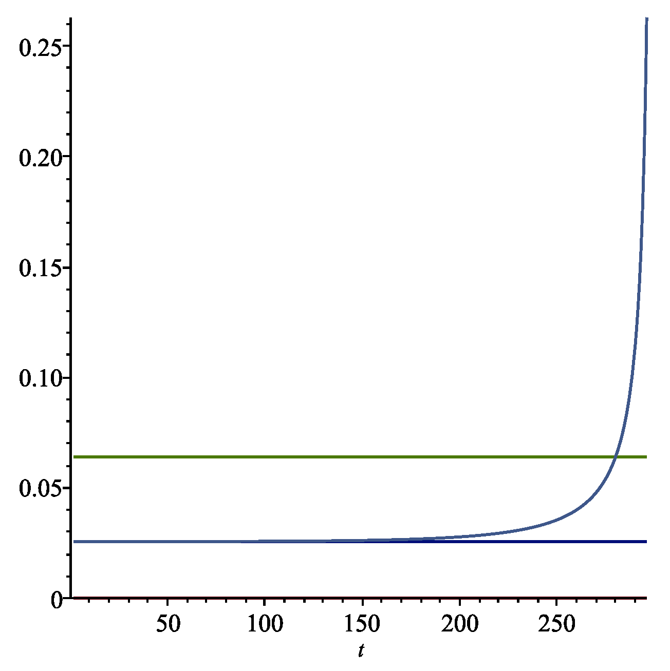
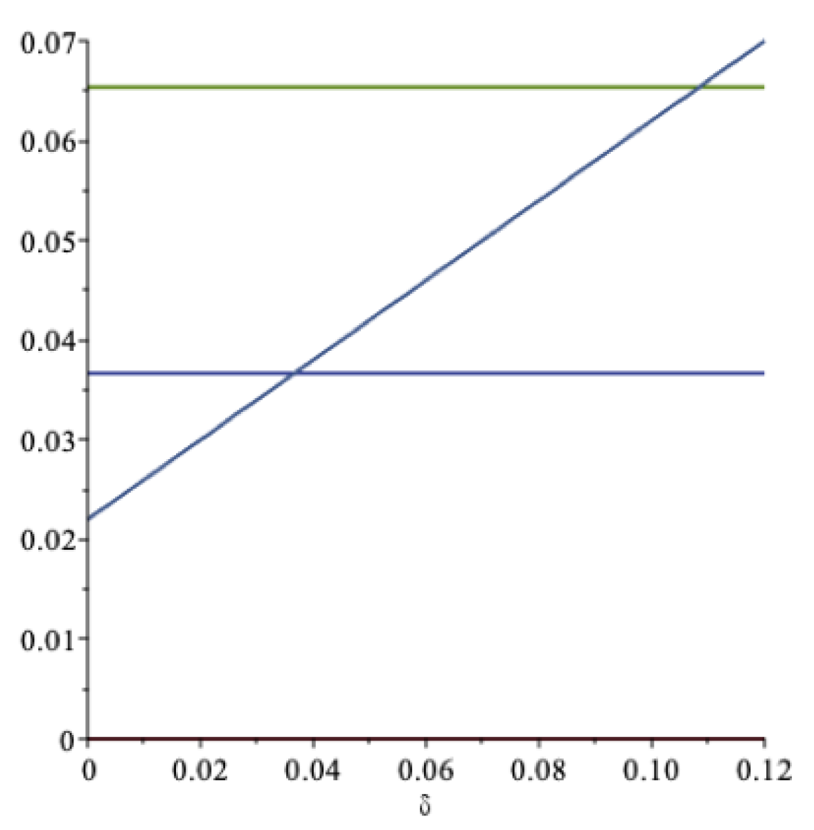
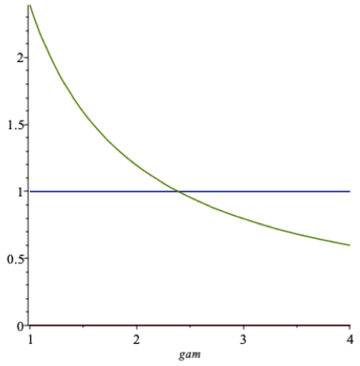
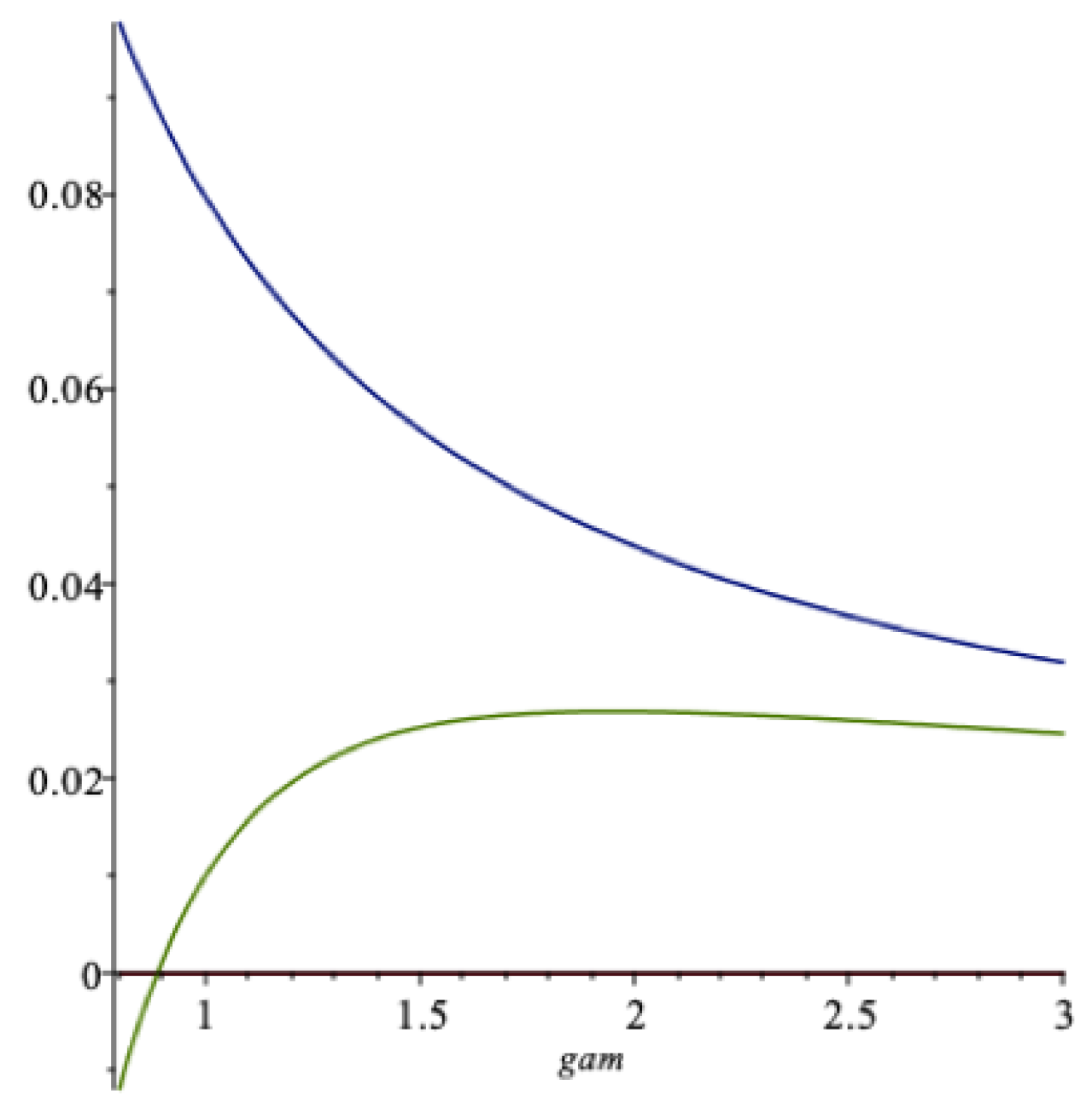
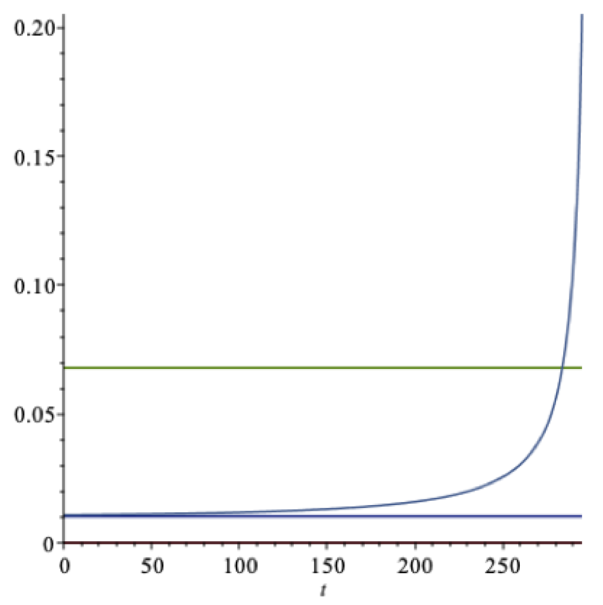
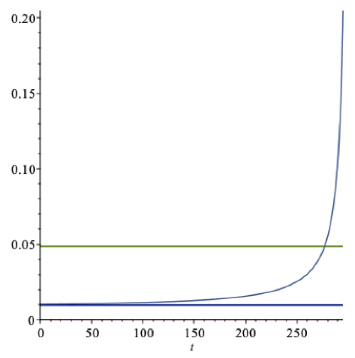
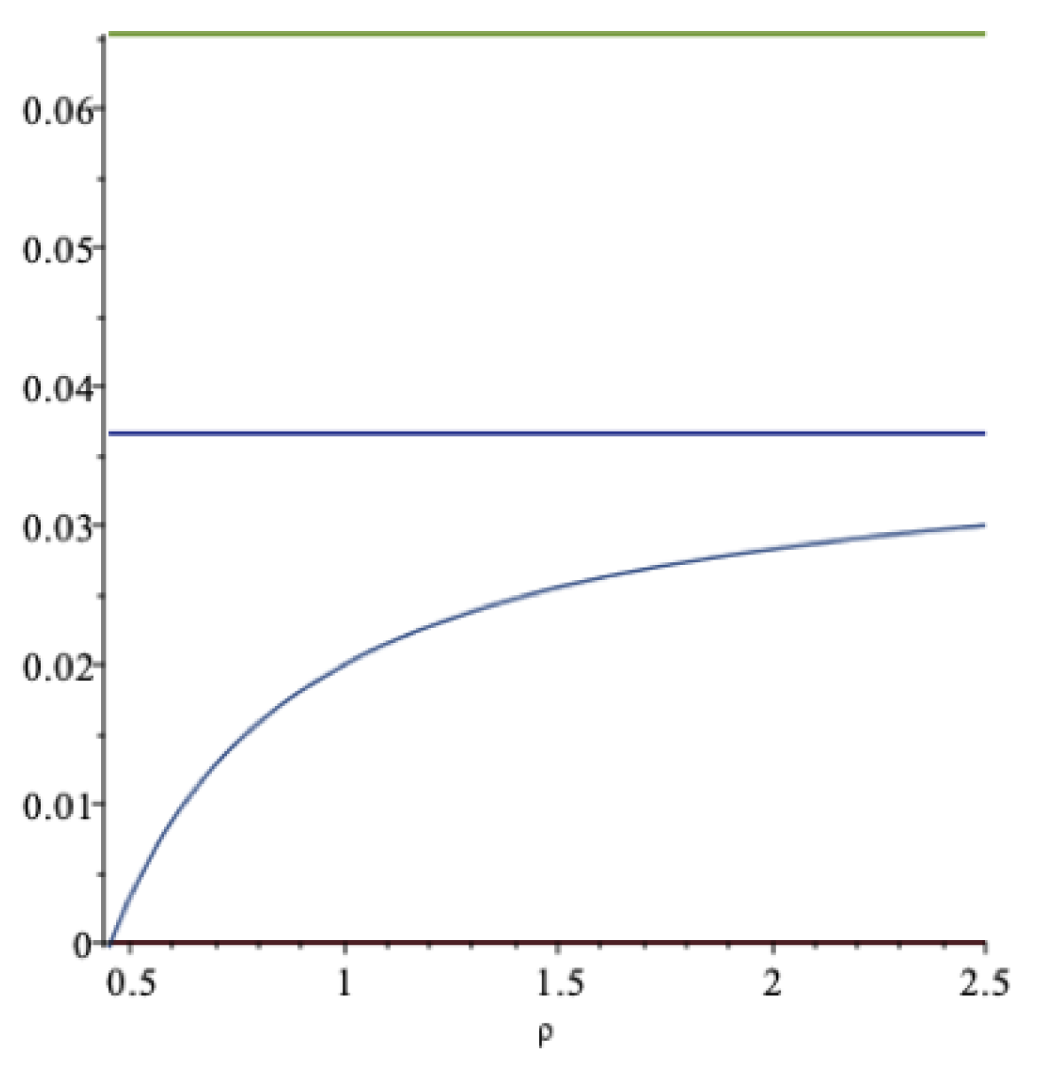
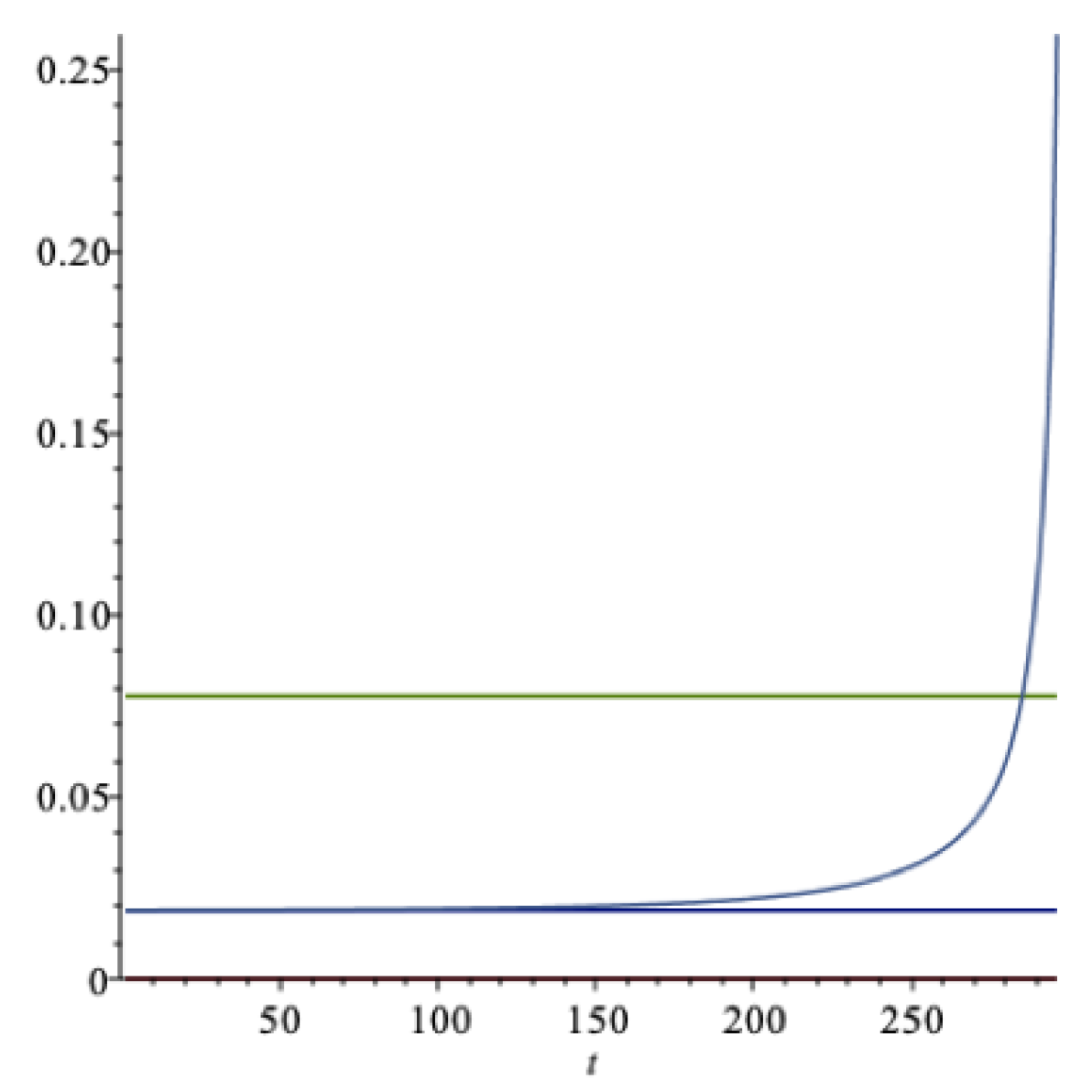
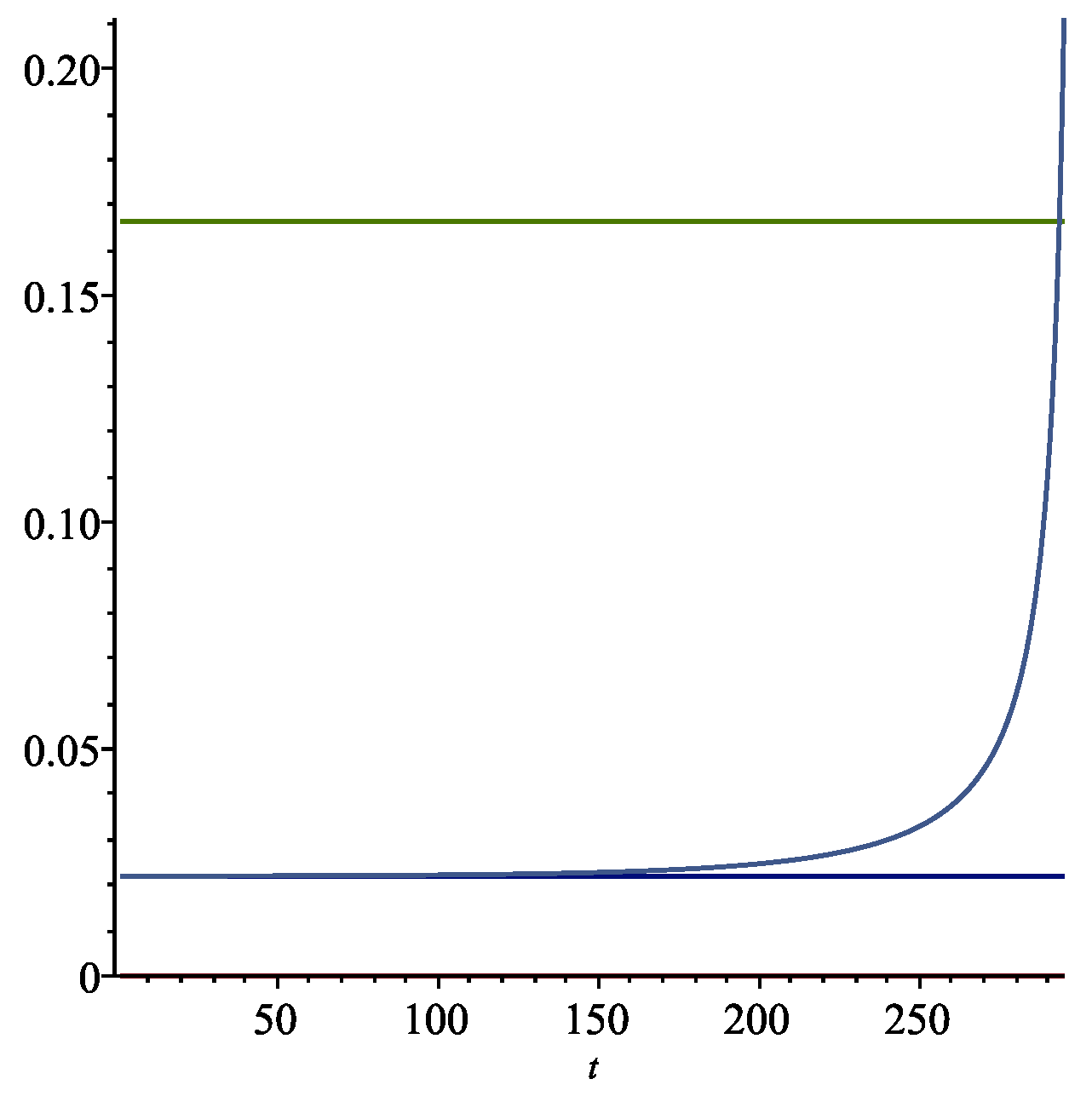
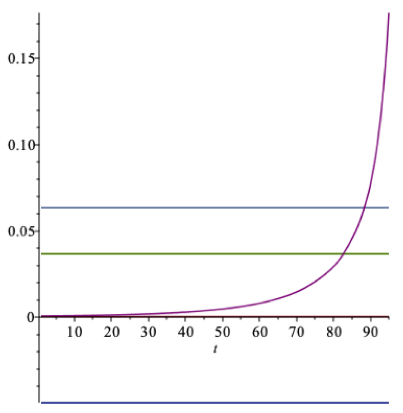
Table 1.
Key US-data for the time period 1889–1978. Continuous-time compounding.
| Expectation | Standard dev. | Covariances | |
|---|---|---|---|
| Return S&P-500 | 6.78% | 15.84% | |
| Government bills | 0.80% | 5.74% | = −0.000149 |
| Equity premium | 5.98% | 15.95% | |
| Consumption growth | 1.81% | 3.55% |
Table 2.
The commission’s market view, Norwegian Ministry of Finance (2016).
Table 2.
The commission’s market view, Norwegian Ministry of Finance (2016).
| Expectation | Standard Dev. | Covariance | |
|---|---|---|---|
| Equity | 4.72% | 16.00% | |
| Bonds | 0.68% | 6.00% | |
| Equity premium | 4.04% | 14.67% |
Publisher’s Note: MDPI stays neutral with regard to jurisdictional claims in published maps and institutional affiliations. |
© 2021 by the authors. Licensee MDPI, Basel, Switzerland. This article is an open access article distributed under the terms and conditions of the Creative Commons Attribution (CC BY) license (https://creativecommons.org/licenses/by/4.0/).
Share and Cite
MDPI and ACS Style
Aase, K.K.; Bjerksund, P. The Optimal Spending Rate versus the Expected Real Return of a Sovereign Wealth Fund. J. Risk Financial Manag. 2021, 14, 425. https://0-doi-org.brum.beds.ac.uk/10.3390/jrfm14090425
AMA Style
Aase KK, Bjerksund P. The Optimal Spending Rate versus the Expected Real Return of a Sovereign Wealth Fund. Journal of Risk and Financial Management. 2021; 14(9):425. https://0-doi-org.brum.beds.ac.uk/10.3390/jrfm14090425
Chicago/Turabian StyleAase, Knut K., and Petter Bjerksund. 2021. "The Optimal Spending Rate versus the Expected Real Return of a Sovereign Wealth Fund" Journal of Risk and Financial Management 14, no. 9: 425. https://0-doi-org.brum.beds.ac.uk/10.3390/jrfm14090425