
Time-Varying Risk and the Relation between Idiosyncratic Risk and Stock Return


School of Business, Faculty of Business and Economics, University of Northern British Columbia, 3333 University Way, Prince George, BC V2N 4Z9, Canada
J. Risk Financial Manag. 2021, 14(9), 432; https://0-doi-org.brum.beds.ac.uk/10.3390/jrfm14090432
Submission received: 16 July 2021
/
Revised: 2 September 2021
/
Accepted: 6 September 2021
/
Published: 9 September 2021
(This article belongs to the Special Issue Financial and Panel Data Econometrics)
Abstract
:This paper studies the historical time-varying dynamics of risk for individual stocks in the U.S. market. Total risk of an individual stock is decomposed into two components, systematic risk and idiosyncratic risk, and both components are studied separately. We start from the historical trend in the magnitude of risk and then turn to the relation between idiosyncratic risk and stock returns. The result shows that both components of risk for individual stocks are changing over time. They increased from the 1960s to the 1990s/2000s and then declined until today. This paper also studies the risk-return tradeoff by investigating the relation between idiosyncratic risk and stock return in the long run. Stocks are sorted into portfolios for analysis and the whole sample period is further decomposed into decades for subgroup analysis. Multivariable regressions are used to study this relation as we control for beta, size, book-to-market ratio, momentum and liquidity. From a historical point of view, we show that the relation between idiosyncratic risk and stock return is time-varying, and it did not exist in certain decades. The results indicate that the risk-return tradeoff also varied in history.
JEL Classification:
G11; G121. Introduction
The risk-return tradeoff is an important topic for investors and researchers in finance. After the Markowitz modern portfolio theory (Markowitz 1952), it is agreed that investors care only about systematic risk in theory as the idiosyncratic risk can be eliminated by holding a well-diversified portfolio. While there is a debate about how to measure the systematic risk, empirical results in the literature also show that idiosyncratic risk plays an important role in affecting stock returns. A lot of studies in the literature have investigated the two components, systematic and idiosyncratic, of risk in stock market such as measuring systematic stock return using factor models (e.g., Fama and French 1992), modeling stock return with conditional models (e.g., Ferson and Harvey 1999), tracking market volatility over time (e.g., Schwert 1989) as well as exploring the effect of idiosyncratic risk on stock returns (e.g., Ang et al. 2006).
As risk is so important for investors, a lot of studies in the literature attempt to model and forecast risk. For example, Andersen et al. (2001) studied the distribution of realized stock return volatility and found that realized volatility and correlation move together. Lu and Perron (2010) used a random level shift model in modeling and forecasting stock return volatility. Molnar (2016) employed a GARCH (1,1) model to improve the out-of-sample volatility forecasting ability. Kambouroudis et al. (2016) focused on the information content of implied volatility forecasts for stock index. Moreover, other studies link risk to important firm characteristics. For example, Harjoto and Jo (2015) found that the corporate social responsibility reduces analyst dispersion of stock return volatility. Pan et al. (2015) show that CEO ability is closely related with risk. They find evidence that the uncertainty about CEO ability contributes to stock return volatility. Adam et al. (2015) used consumption-based asset pricing models to generate stock price volatility.
To further understand risk in the financial market, some studies in literature extend the scope of risk study to international area. In a study of 31 emerging markets, Li et al. (2011) found a negative relation between large foreign ownership and stock return volatility. Moreover, Chen et al. (2013) present evidence that foreign institutional ownership increases stock return volatility in the Chinese stock market. Vo and Ellis (2018) show a volatility linkage between Vietnamese stock market with other leading equity markets of the U.S., Hongkong and Japan. Li et al. (2005) found a positive but insignificant relationship between stock returns and volatility in the 12 largest international stock markets. On the other hand, a few studies link risk with investor behavior. For example, Behrendt and Schmidt (2018) used information from stock-related Tweets to construct an investor sentiment measure. They show that the intraday volatility co-moves with the investor sentiment.
However, none of the studies start from the risk of individual stocks in a historical perspective. We attempt to fill the gap in this study. The change of pattern for risk in the long run will reveal ample information about the risk itself and the risk-return tradeoff. We are also motivated by the historical panel data on the U.S. stock returns and the methodology used by Ang et al. (2006) that allows us to estimate systematic risk and idiosyncratic risk for individual stocks. The research questions in this study are: (1) what is the historical trend of stock risk, and (2) how does the relation between idiosyncratic risk and return change over time? Using the historical data from 1963 to 2019, we explore how each component of risk changes in the long run to answer the first question. Moreover, we describe the systematic risk and idiosyncratic risk of individual stocks for each decade within the sample period. Such analysis helps to discover the time trend in stock risk. Moreover, we explore the second questions by investigating the historical trend in the relation between idiosyncratic risk and stock returns. Both portfolio analysis and cross-sectional regression analysis are used. The analysis provides detailed results about this relation on a portfolio level and on an individual stock level.
The historical trend of risk of individual stocks is important for investors. Few studies in the literature discuss the risk-related issues in the long run and find them insightful. Using an international data of 200 years, Danielsson et al. (2018) found that stock market volatility has an effect on risk-taking. Low market volatility leads to more risk taken by agents. Bodie (1995) studied whether investing in common stocks is less risky for an investor with longer holding horizon. He found this proposition is wrong in the real world. Chiang and Li (2012) investigated the relation between risk and return using high frequency data. Aslanidis et al. (2021) studied the risk-return tradeoff with a focus of tails of the stock returns. Other studies focus on the interaction between volatility and returns and on the predictability of stock returns by risk. For example, Zumbach (2010) found that trending stock prices lead to increased realized volatility. These studies in the literature build up, as what we conduct in this study, the risk-return tradeoff in the stock market. To our knowledge, this is the first study that explores the historical risk-return tradeoff for individual stocks.
There are two components of risk, systematic risk and idiosyncratic risk. We focus on the relation between idiosyncratic risk and stock return because this relation seems puzzling to researchers. Based on the Markowitz modern portfolio theory (Markowitz 1952), investors hold a well-diversified portfolio, and the idiosyncratic risk will be eliminated. Investors will be compensated by bearing only systematic risk. However, Ang et al. (2006) found a significantly negative relation between idiosyncratic risk and stock return. The empirical result seems puzzling as it contradicts to the theory. Studies in the literature follow Ang et al. (2006) and investigate why such a relation exists. For example, Huang et al. (2010) argue that the negative relation is mainly driven by return reversal. Stambaugh et al. (2015) present evidence that arbitrage asymmetry explains the relation. Cao et al. (2008) suggest that growth options can explain the trend in idiosyncratic volatility. Han and Lesmond (2011) demonstrate that liquidity bias is the driving factor of the ability of idiosyncratic volatility to predict future returns. Moreover, Cao and Han (2013) show a robust negative relation between delta-hedged equity option return and idiosyncratic risk of underlying stock. Overall, the results seem mixed, and no consensus has been reached yet.
Additionally, some studies in the literature attempt to deepen the understanding of idiosyncratic risk. For example, Bekaert et al. (2012) show that the aggregate idiosyncratic risk is highly correlated across 23 developed equity markets. Fu (2018) present evidence that the time-varying alpha is a component of idiosyncratic risk, and it negatively relates with stock returns. Other studies in the literature attempt to link idiosyncratic risk with other important issues in finance. For example, Becchetti et al. (2015) show that idiosyncratic risk is positively related with aggregate corporate social responsibility. Aabo et al. (2017) argue that idiosyncratic volatility seems to be an indicator of noise trading. Huang et al. (2015) and Vo and Phan (2019) found consistent evidence that idiosyncratic volatility is linked with herding behavior in different markets. In a comprehensive study, Hou and Loh (2016) attempt to explain the puzzling relation by summarizing the effects of several potential factors and they argue that “all existing explanations still leave a sizable portion of the puzzle unexplained”. Therefore, the investigation on the relation between idiosyncratic risk and return is still not conclusive and we attempt to add to the exploration of this puzzling relation from a historical point of view.
This study is also motivated by Cao et al. (2021). In the recent study, Cao et al. (2021) show that the negative relation between idiosyncratic risk and return exhibits strong calendar effects. They found that the puzzling relation is generally negative on Mondays but positive on Fridays. Their results suggest that the relation between idiosyncratic risk and return is not the same over time. However, our study is different from Cao et al. (2021) in that our study focuses on decades in history, and they focused on the calendar from Monday to Friday. Moreover, we are more concerned about the time trend instead of a certain point of time. On the other hand, in another study, Herskovic et al. (2016) found a common factor in idiosyncratic volatility. If this is true, it implies that both components of risk co-move over time. To the best of our knowledge, this paper is the first study that investigates the historical time-varying relation between idiosyncratic risk and return.
This study has two main contributions. First, it contributes to the literature by showing the historical dynamics of systematic risk and idiosyncratic risk for individual stocks. Instead of estimating the market level volatility, we show that both components of risk for individual stocks change over time. Stock risk grew from the 1960s to its peaks in the 1990s and 2000s, and then declined until today. It adds value to the literature that predicts stock market risk and improves investment decision making. Second, this study extends the understanding of the relation between idiosyncratic risk and stock returns. The empirical results of portfolio analysis and regression analysis indicate that the relation changes over time. It implies that the risk-return tradeoff is not stable as it shrinks in several periods of time in history. This study conducts a subperiod analysis of the relation between idiosyncratic risk and stock returns. The results show that the significance of the relation between idiosyncratic risk and stock return is negatively related with the level of idiosyncratic risk. The negative relation is significant when the level of idiosyncratic risk is low, and it becomes insignificant when the level peaks. The findings deepen the understanding of stock risk and provide insights for future studies in the risk-return tradeoff. Overall, the contribution of this study adds to the literature of risk-return tradeoff and helps researchers and investors understand the time-varying dynamics of each component of risk in the long run. This study is structured as follows. Section 2 presents the data and methodology. Section 3 provides empirical results. Section 4 concludes.
2. Data and Methodology
We built the sample from the Center for Research in Security Prices (CRSP) common shares traded on the New York Stock Exchange (NYSE), American Stock Exchange (AMEX) and NASDAQ from July 1963 to December 2019. The daily and monthly stock returns are obtained from the CRSP. Following Fu (2009), stocks with monthly returns greater than 300 percent are excluded from the sample. The accounting data are collected from the Compustat database. The Fama–French factors are downloaded from Professor French’s website1.
The idiosyncratic risk of stock return is estimated in the same way as Ang et al. (2006). Within each month, daily stock returns are regressed on the Fama–French three factors. A stock should have at least 15 days of returns in a month to be included in the calculation. The following Equation (1) shows the process of idiosyncratic risk estimation.
where is excess return of stock i at day t. , and are the Fama and French (1992) three factors. ε is the residual term used to calculate idiosyncratic volatility. The monthly idiosyncratic risk for an individual stock is the standard deviation of the residual term ε multiplied by the square root of number of trading days in that month. This method is also used by many following studies in the literature such as Huang et al. (2010), Han and Lesmond (2011) and Hou and Loh (2016).
Then, the systematic risk is calculated by subtracting the idiosyncratic risk from total risk, which is calculated as the standard deviation of stock returns multiplied by the square root of number of trading days in that month. The process is given in Equation (2) below.
where is the total risk and and are the two components of risk. Rearranging Equation (2) gives Equation (3) below, which shows the calculation of systematic volatility.
where the idiosyncratic risk is calculated as in Equation (1).
Next, we started the analysis with portfolio formation. The main reason for portfolio formation is to eliminate noise in the idiosyncratic volatility of individual stock returns. On a portfolio level, it helps to observe any pattern in the relation between idiosyncratic risk and stock returns. As small size stocks usually come with high level of firm-specific risk2 (i.e., idiosyncratic risk), we conducted a double sorting to make sure size is control for when analyzing the relation on a portfolio level. A similar method is used in other studies such as Ang et al. (2006), Han and Lesmond (2011) and Cao and Han (2013).
In the portfolio analysis, stocks are first sorted into five size quintile portfolios based on its size on month t and then each size quintile is further sorted into five quintiles based on idiosyncratic risk on month t. As a result, it gives the 5 × 5 portfolios. Each portfolio is held by another month and the holding period return is calculated on month t + 1. This portfolio sorting process makes sure the size and idiosyncratic risk are observable when forming the portfolios so that the looking forward bias is eliminated. As size is the most important stock characteristic that is related with idiosyncratic risk, this portfolio sorting assures that the relation is studied within portfolios of stocks with similar size. In other words, portfolio analysis mitigates the concern that our results are affected by size.
Finally, we employed the firm-level Fama and MacBeth (1973) regressions as described in the following Equation (4).
where is the excess return of stock i on month t. is the idiosyncratic risk of stock i at month t. Controls is the vector of controlling variables including beta, size, book to market ratio, momentum and liquidity. Size and book to market ratio (B/M) are calculated following Fama and French (1992). Stock-level market beta (Beta) is estimated from 60-month rollover regressions. Momentum is calculated as the compound gross return from month (t − 7) to (t − 2). The average volume turnover (TURN) and coefficient of variance of volume turnover (CVTURN) are calculated over the past 36 months following Chordia et al. (2001). TURN and CVTURN are the liquidity-related controlling variables. Additional description of control variables can be found in the corresponding tables. The periods of economic recession and boom are collected from National Bureau of Economic Research (NBER) website3 of business cycle dates.
3. Empirical Results
In this section, we describe the empirical results of historical trend in stock risk. To start with, we analyze the systematic risk and idiosyncratic risk estimated from the panel data of stock returns. Then, a portfolio analysis is conducted to show how the relation between idiosyncratic risk and stock returns changes over time. Finally, we present the results of Fama and MacBeth (1973) regressions and conduct several robustness tests on such relation.
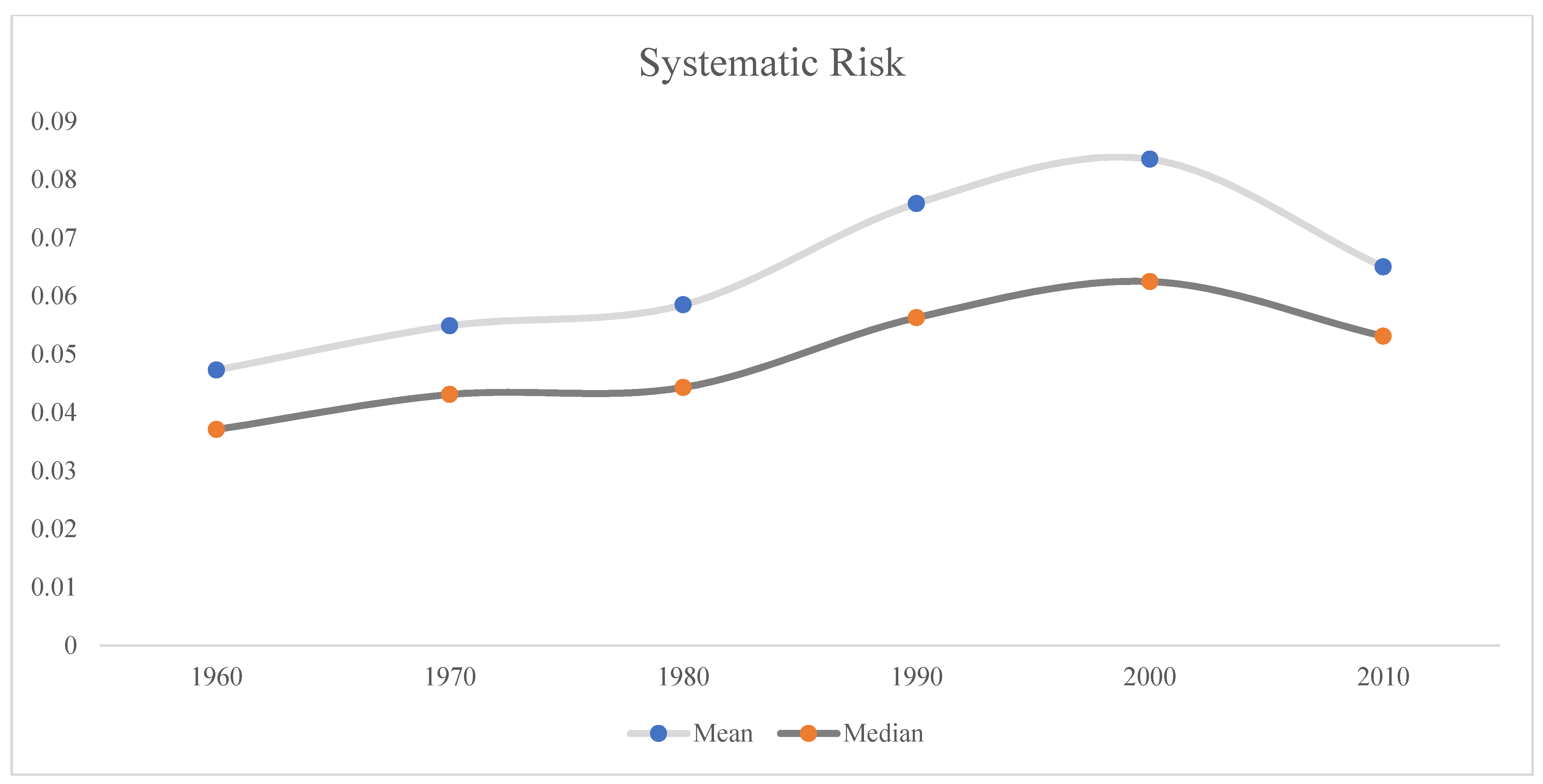
Table 1 is the descriptive statistics of systematic risk on stock returns. Within the whole sample period, the average systematic risk of all stocks is 0.0661 and the standard deviation is 0.0637. The total number of monthly observations after data filtering is about 3 million. The following portion of the table describes the systematic risk in each decade. We observe that the mean of systematic risk increased from the 1960s to the 2000s and then dropped in the 2010s. This is also true for the median and standard deviation of systematic risk. While systematic risk was reduced in the 2010s, it is still on a higher level comparing with the periods before the 1980s. This historical patten of systematic risk is depicted in Figure 1. It is clear that the mean and median of systematic risk co-moves in a similar way. In sum, the systematic stock risk is not nonchanging from a historical point of view.
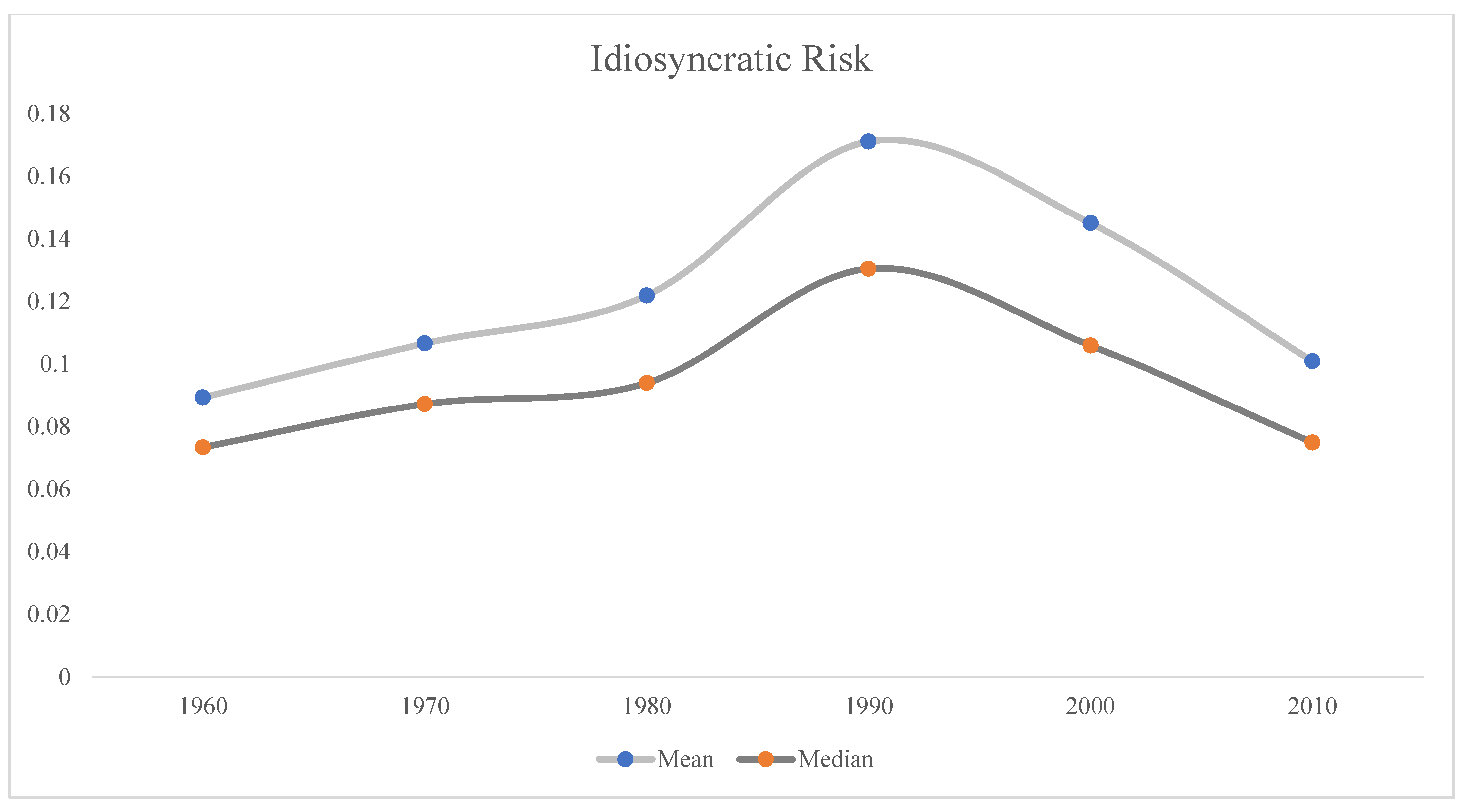
The description of idiosyncratic risk on stock returns is presented in Table 2. The average idiosyncratic risk is 0.1298 for the whole sample period, higher than the average systematic risk of 0.0661 in Table 1. The median (0.0967) is lower than the mean (0.1298), showing that idiosyncratic risk is not normally distributed. Then, the descriptive statistics of idiosyncratic risk for each decade is reported. Again, we observe that the idiosyncratic risk is not stable as it changes over time. Similar to the pattern of systematic risk, the average idiosyncratic risk grew until the 1990s and then started to decline in the 2000s. In the 2010s, the average level of idiosyncratic risk was close to that of the 1960s and 1970s when it started to grow. Figure 2 depicts such historical trend for the mean and median of idiosyncratic risk that co-moves in a same pattern. Given the previously discussed results of systematic risk, we conclude that risk of individual stocks changes in history. This is true for both systematic risk and idiosyncratic risk. In today’s stock market, both components of stock risk are experiencing a shrink.
Our results are consistent with Fink et al. (2010) in that aggregate idiosyncratic risk increased during the Internet boom. These results are also supportive of Campbell et al. (2001) in that there was a positive trend in idiosyncratic volatility between 1962 and 1997. It seems to be partially explained by the changes in the business cycles of the U.S. economy. The economy experiences ups and down from a historical point of view, as does the risk on the U.S. stock market. Risk tends to be high in certain periods in history and then tends to decline. The critical point is close to the 1990s, when the dot-com bubble emerged as it eventually became the largest bubble in the U.S. stock market history. This possible explanation is from Bekaert et al. (2012) as they show evidence that the trend in aggregate idiosyncratic volatility could be attribute to a business cycle sensitive risk indicator. Another possible explanation for this phenomenon is the time varying maturity of firms in the U.S. stock market. As argued by Fink et al. (2010), market-wide decline in maturity of the typical public firm can explain most of the increase in idiosyncratic risk during the Internet boom. If this is true, the decline trend in the 2000s and 2010s could be attributed to an increase in maturity of public firms because companies who experienced the dot-com bubble tend to be more careful when making financial decisions4. It is possible that more companies tend to survive from following economic downturn and live longer today as they are learning from the lesson of the dot-com bubble. As a result, we observe a decline in risk in the stock market after the dot-com bubble.
As we show the historical trend of stock risk, it will not be surprising to extend our study on the risk-return trade off. Specifically, we are interested in how the relation between stock risk and return develops in history. In this study, we focus on the relation between idiosyncratic risk and stock returns because it is puzzling and seems more interesting to researchers. As we estimate the idiosyncratic risk of individual stocks for a long period of time, it becomes feasible for us to investigate the relation in a historical perspective. Because the levels of both components of risk are time-varying in history, one could expect that the risk-return tradeoff also changes over time.
Table 3 presents the results of portfolio analysis of the relation between idiosyncratic risk and stock returns. In each month, all stocks are sorted into five quintile portfolios based on their size (market capitalization) and then stocks in each portfolio are further sorted into five portfolios based on their idiosyncratic risk. As a result, 25 portfolios are obtained. Instead of one-month portfolio returns, risk-adjusted portfolio returns are reported. The Fama–French 3-factor alpha, portfolio return adjusted by Fama–French 3 factors, is then calculated equally weighted and reported in the table. Given a size quintile, we calculated the monthly long-short portfolio strategy alpha by taking a long position of the portfolio with the highest idiosyncratic risk and a short position of the one with the lowest idiosyncratic risk. The t-values are reported in the parentheses. For the whole sample period, we observed a negative long-short portfolio strategy alpha ranging from −0.41 to −1.21, all statistically significant. It indeed supports the negative relation between idiosyncratic risk and stock return on a portfolio level. This is consistent with studies in the literature.
Then, a subperiod analysis was conducted for each decade. The results are different from that of the whole sample period. For example, in the 1960s, four out of the long-short portfolio strategy alphas are statistically insignificant, showing that the negative relation between idiosyncratic risk and stock return is minimum in that period. While not significant, we found a positive long-short portfolio strategy alpha of 0.32 for stocks in the second largest size quintile. Moreover, there is a similarly marginal relation in the 1990s and 2000s when the level of idiosyncratic risk is high as discussed earlier. This is surprising as the results indicate that the negative relation is mainly driven by small stocks and such relation is close to none in the subperiods when idiosyncratic risk is high. Finally, we wanted to see if the relation is affected by the periods of recessions. The results show that there is a significantly negative relation between idiosyncratic risk and stock return in booming periods but not in recessionary periods. Overall, the empirical results in Table 3 show that similar to the historical change in risk, the risk-return relation also changes over time on a portfolio level. The negative relation between idiosyncratic risk and stock return does not exist in the 1960s and the periods when the level of idiosyncratic risk is high. It also disappears in large and middle size stocks in certain periods.
The result on portfolios analysis is generally consistent with what we expect as the level of risk changes over time. As time passes in history, it shows that the relation between idiosyncratic risk and stock return is not stable on a portfolio level. One possible explanation is in spirit of the change in business cycle discussed by Bekaert et al. (2012). They show that the trend in aggregate idiosyncratic volatility could be attribute to a business cycle sensitive risk indicator. If this is true, one could expect that the business cycle may also affect the relation between idiosyncratic risk and stock returns over time. However, additional tests are needed to verify this expectation. On the other hand, the result also implies that the systematic component of risk becomes more dominant in determining stock returns in some periods. For example, in the periods of the 1990s, both systematic risk and idiosyncratic risk peaked at a historical high. Although not tested in this study, one could project that the stock returns are more associated with the systematic risk in that period because the relation between idiosyncratic risk and returns disappears. In other words, the investor could hardly use information from firm-specific risk to trade in that period of time. It is possible that herding behavior discussed by Huang et al. (2015) and Vo and Phan (2019) plays a role in this period. In the 1990s, investors “followed the crowd” to buy any stocks that were related to the Internet in the market. If investors ignored firm-specific risk information, it is possible that the relation between idiosyncratic risk and stock return became minimum.
While we provided evidence that the risk-return trade off changes over time on a portfolio level, one may want to see if this holds on an individual stock level. Moreover, only size and idiosyncratic risk are controlled in portfolio sorting, one may ask if the relation is still time-varying by adding more control variables. To answer this question, the Fama and MacBeth (1973) cross-sectional regressions were used to study the relation between idiosyncratic risk and stock returns. Several control variables were considered including beta, size, book-to-market ratio, momentum and turnover. Table 4 shows the correlation matrix of the controlling variables. It is observable that the controlling variables are not highly correlated with each other. However, there is one pair of variables, size and coefficient of variance of turnover (CVTURN), that has a correlation of −0.44. It suggests that collinearity may be a concern in the following regression tests and additional diagnostic test are required.
Table 5 presents the results of regressions described in Equation (4). The coefficient of idiosyncratic risk is the most important variable as it tells its relation with stock returns. In the whole sample period, the coefficient is −0.042, indicating that a 1 percent increase in idiosyncratic risk is associated with 0.04 percent decrease in monthly stock returns. This relation is statistically significant as the Newey–West adjusted t-value is −6.95.
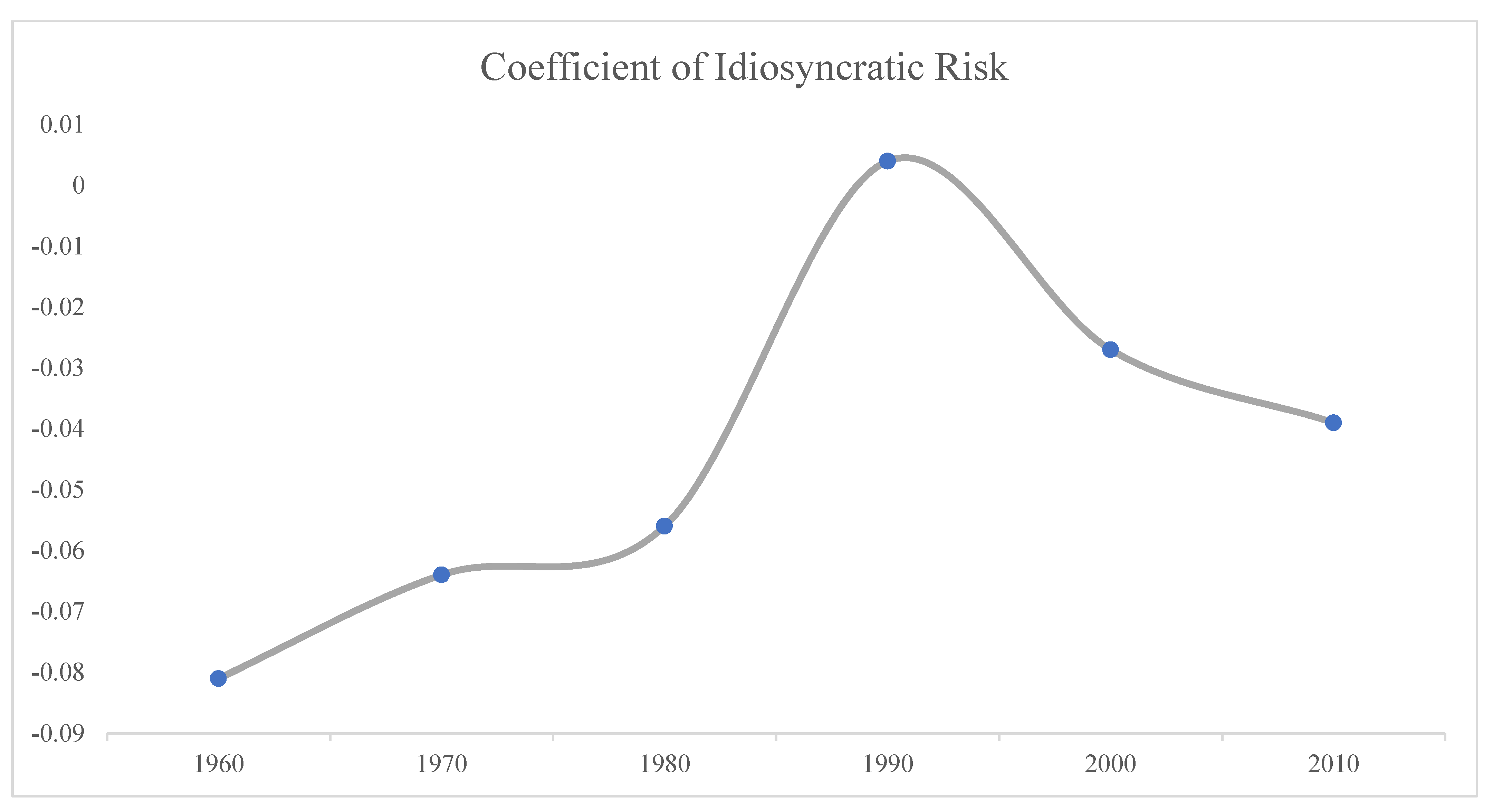
Next, the regression results of subperiods show a time-varying relation, but it tells a slightly different story than that in portfolio analysis. In the 1960s, there was a significantly negative relation between idiosyncratic risk and stock return. This is different from the results on a portfolio level. We observe a similar negative relation for all decades except 1990s when the coefficient was statistically insignificant at 0.004. It is noticeable that the negative relation was strong in the 1960s and then became weaker until the 1990s. After this decades, the negative relation restored until the 2010s. Such trend is demonstrated in Figure 3. To conclude, the time-varying relation on an individual stock level is not identical to that on a portfolio level. Comparing with the pattern of average idiosyncratic risk in history, we conclude that the significance of the relation between idiosyncratic risk and stock return is negatively associated with the level of idiosyncratic risk. That is, the relation is strong (weak) when market average idiosyncratic risk is low (high). Finally, there is no difference between recession and boom in terms of the relation between idiosyncratic risk and stock return.
As discussed before, one needs to be cautious in interpreting the results by addressing the potential collinearity in the control variables. Thus, we conduct a variance inflation factor (VIF) to check for collinearity. In the regression for the whole sample period, we find that the tolerance for size and CVTURN are 0.33 and 0.40, respectively. Both of them are greater than the threshold 0.1. Comparably, we found that the VIF for size and CVTURN are 2.99 and 2.51, respectively. Again, both factors are less than the threshold 10, indicating these two variables in the regressions are fine. The VIF results also show that other variables are not subject to collinearity. Then, we conducted the VIF diagnosis for each subperiod and subgroup analysis; the results are similar. Overall, the VIF results suggest no collinearity concerns in our models.
Is it possible that the results are affected by other pricing models in estimating idiosyncratic risk? To address this concern, we used different factor models (i.e., CAPM, Carhart (1997), and Fama and French (2015) five factor model) to estimate idiosyncratic risk and investigate its relation with stock return in history. Those additional tests will show if our results are robust in the selection of factor models when calculating idiosyncratic risk. The results of these tests are presented in Appendix A Table A1, Table A2 and Table A3. When idiosyncratic risk is estimated by different pricing models, we observe a similar pattern of the historical risk-return tradeoff. In the 1990s, the negative relation was weak but it is significant in all other decades.
As Olbrys (2021) summarizes that the global financial crisis (GFC) had a significant impact on the stock market; we also considered additional robustness tests by excluding business contraction periods of the great financial crisis (GFC) or the dot-com bubble period. The regression test results are presented in Appendix A, Table A4. In general, the results show that GFC has minimal effect on the relation between idiosyncratic risk and stock returns. This result is consistent with the results in Table 5 that recession and boom periods have almost the same relation between idiosyncratic risk and stock returns. However, when we consider the dot-com bubble only, the negative relation becomes insignificant. This is in support of the results in Table 5 that the relation did not exist in the 1990s.
In sum, our results indicate that the relation between idiosyncratic risk and stock return is not always the same, as suggested by previous studies. It also implies that investors and researchers need more understanding about the relation in history. This implication is consistent with Hou and Loh (2016), who assert that there is still a lot of unknown in the relation between idiosyncratic risk and stock return. The business cycle is one of the potential explanations for the time-varying relation as both the risk level and its relation with return changes in a historical point of view.
4. Conclusions
In this study, we estimated the systematic and idiosyncratic components of risk for individual stocks. We analyzed them in the historical trends and found that both components of risk change over time. The systematic risk and idiosyncratic risk increased from the 1960s to the 1990s and the 2000s and then started to drop until the 2010s. Then, the relation between idiosyncratic risk and stock return was investigated. We used both portfolio analysis and cross-section regressions and found that the relation also changes in different decades in history. On a portfolio level, the puzzling relation did not exist in the 1960s, 1990s, 2000s and the recessionary period. On an individual stock level, the negative relation disappeared in the 1990s. Moreover, we found that the relation between idiosyncratic risk and stock return is strong (weak) when market average idiosyncratic risk is low (high). There is no difference of this relation between recession and boom in history.
The findings in this study are important for investors in the U.S. stock market. It provides evidence about the effectiveness of portfolio diversification. Investors will learn from this study in terms of the compensation for bearing systematic risk and idiosyncratic risk. It is more beneficial for long term investors as this study reveal the historical change in the risk-return tradeoff. Investors can learn from the historical trends and patterns in the risk-return tradeoff to generate new trading strategies and predict future stock returns. For example, investors can compare the current risk in the market with historical median or mean risk and then take action to adjust their exposure to the risk and trading strategy. Moreover, this study will also benefit researchers in the puzzling relation between idiosyncratic risk and returns. It adds to the findings of Hou and Loh (2016) and Cao et al. (2021). This study provides new insights in the relation between idiosyncratic risk and stock returns. Future research could be done on the reasons of the time-varying risk and risk-return tradeoff.
Funding
This research received no external funding.
Institutional Review Board Statement
Not applicable.
Informed Consent Statement
Not applicable.
Data Availability Statement
Data available on request.
Conflicts of Interest
The authors declare no conflict of interest.
Appendix A

Table A1.
This table reports the regression results of robustness tests when idiosyncratic risk is estimated by CAPM model. It reports the results of the firm-level Fama and MacBeth (1973) regressions of monthly stock returns on idiosyncratic risk for the period of July 1963 to December 2019. A stock should have at least 15 daily returns in a month to be included in the risk estimation. Stock-level market beta is estimated from 60-month rollover regressions. ME Size and B/M are size and book-to-market ratio in Fama and French (1992). Momentum is the compound gross return from month (t − 7) to (t − 2). TURN and CVTURN are the average volume turnover and coefficient of variance of TURN calculated over the past 36 months in Chordia et al. (2001). The idiosyncratic risk (Idio) is the standard deviation of regression residuals of daily stock returns in month t − 1. The Newey–West adjusted t-value is reported in parentheses. To avoid the effect of possibly spurious outliers, all explanatory variables below 0.1 (above 99.9) percentile are set equal to 0.1 (99.9) percentile. *, ** and *** denote the statistical significance level at 10%, 5% and 1%, respectively.
| Whole Period | 1960s | 1970s | 1980s | 1990s | 2000s | 2010s | |
|---|---|---|---|---|---|---|---|
| Intercept | 1.480 *** | 1.141 | 1.591 ** | 1.311 ** | 0.565 | 2.095 *** | 2.032 *** |
| (5.52) | (1.56) | (2.13) | (1.77) | (0.98) | (3.61) | (4.39) | |
| Idio | −0.040 *** | −0.072 *** | −0.069 *** | −0.048 *** | 0.002 | −0.025 * | −0.037 *** |
| (−6.05) | (−3.11) | (−4.33) | (−4.94) | (0.18) | (−1.78) | (−3.62) | |
| Beta | 0.430 *** | 0.205 | 0.740 * | 0.448 | 0.545 | 0.223 | 0.171 |
| (2.72) | (0.63) | (1.82) | (1.04) | (1.30) | (0.51) | (0.67) | |
| Size | −0.177 *** | −0.312 *** | −0.253 *** | −0.015 | −0.218 *** | −0.177 *** | −0.082 |
| (−5.21) | (−3.54) | (−2.82) | (−0.16) | (−2.65) | (−2.39) | (−1.56) | |
| B/M | 0.170 *** | 0.025 | 0.161 | 0.397 *** | 0.154 | 0.184 | −0.024 |
| (3.67) | (0.52) | (1.17) | (4.40) | (1.20) | (1.55) | (−0.24) | |
| Momentum | 0.773 *** | 1.586 *** | 0.622 | 0.544 ** | 1.290 *** | 0.327 | 0.270 |
| (5.74) | (4.20) | (1.56) | (2.22) | (4.34) | (1.16) | (1.07) | |
| TURN | −0.208 *** | 0.025 | −0.162 | −0.383 *** | −0.212 * | −0.052 | −0.310 *** |
| (−4.41) | (0.16) | (−1.58) | (−4.78) | (−1.78) | (−0.46) | (−3.73) | |
| CVTURN | −0.331 *** | −0.174 | −0.273 *** | −0.092 | −0.805 *** | −0.391 ** | −0.391 *** |
| (−5.81) | (−1.14) | (−2.63) | (−0.80) | (−6.62) | (−2.26) | (−3.15) | |
| 0.077 *** | 0.115 *** | 0.087 *** | 0.061 *** | 0.078 *** | 0.077 *** | 0.058 *** | |
| (18.00) | (8.98) | (8.95) | (8.14) | (7.96) | (7.60) | (8.18) |
Table A2.
This table reports the regression results of robustness tests when idiosyncratic risk is estimated by Carhart (1997) model. It reports the results of the firm-level Fama and MacBeth (1973) regressions of monthly stock returns on idiosyncratic risk for the period of July 1963 to December 2019. A stock should have at least 15 daily returns in a month to be included in the risk estimation. Stock-level market beta is estimated from 60-month rollover regressions. ME Size and B/M are size and book-to-market ratio in Fama and French (1992). Momentum is the compound gross return from month (t − 7) to (t − 2). TURN and CVTURN are the average volume turnover and coefficient of variance of TURN calculated over the past 36 months in Chordia et al. (2001). The idiosyncratic risk (Idio) is the standard deviation of regression residuals of daily stock returns in month t − 1. The Newey–West adjusted t-value is reported in parentheses. To avoid the effect of possibly spurious outliers, all explanatory variables below 0.1 (above 99.9) percentile are set equal to 0.1 (99.9) percentile. *, ** and *** denote the statistical significance level at 10%, 5% and 1%, respectively.
| Whole Period | 1960s | 1970s | 1980s | 1990s | 2000s | 2010s | |
|---|---|---|---|---|---|---|---|
| Intercept | 1.449 *** | 1.107 | 1.568 ** | 1.263 * | 0.548 | 2.085 *** | 1.982 *** |
| (5.40) | (1.52) | (2.11) | (1.73) | (0.93) | (3.55) | (4.24) | |
| Idio | −0.041 *** | −0.075 *** | −0.073 *** | −0.050 *** | 0.003 | −0.026 * | −0.038 *** |
| (−5.96) | (−3.31) | (−4.25) | (−4.68) | (0.22) | (−1.77) | (−3.64) | |
| Beta | 0.426 *** | 0.203 | 0.734 * | 0.441 | 0.542 | 0.219 | 0.167 |
| (2.696) | (0.63) | (1.80) | (1.03) | (1.29) | (0.50) | (0.66) | |
| Size | −0.175 *** | −0.311 *** | −0.251 *** | −0.012 | −0.216 *** | −0.176 *** | −0.079 |
| (−5.17) | (−3.53) | (−2.81) | (−0.13) | (−2.64) | (−2.39) | (−1.49) | |
| B/M | 0.171 *** | 0.026 | 0.161 | 0.399 *** | 0.156 | 0.184 | −0.025 |
| (3.68) | (0.54) | (1.17) | (4.42) | (1.22) | (1.56) | (−0.25) | |
| Momentum | 0.780 *** | 1.594 *** | 0.625 | 0.557 ** | 1.292 *** | 0.326 | 0.283 |
| (5.79) | (4.28) | (1.57) | (2.28) | (4.32) | (1.16) | (1.09) | |
| TURN | −0.213 *** | 0.017 | −0.167 | −0.387 *** | −0.213 * | −0.055 | −0.316 *** |
| (−4.49) | (0.11) | (−1.63) | (−4.86) | (−1.78) | (−0.49) | (−3.76) | |
| CVTURN | −0.332 *** | −0.178 | −0.274 ** | −0.091 | −0.808 *** | −0.392 ** | −0.390 *** |
| (−5.81) | (−1.16) | (−2.62) | (−0.80) | (−6.60) | (−2.25) | (−3.17) | |
| 0.077 *** | 0.115 *** | 0.087 *** | 0.061 *** | 0.078 *** | 0.078 *** | 0.057 *** | |
| (18.02) | (8.97) | (8.94) | (8.12) | (7.99) | (7.61) | (8.27) |
Table A3.
This table reports the regression results of robustness tests when idiosyncratic risk is estimated by Fama and French (2015) five factor model. It reports the results of the firm-level Fama and MacBeth (1973) regressions of monthly stock returns on idiosyncratic risk for the period of July 1963 to December 2019. A stock should have at least 15 daily returns in a month to be included in the risk estimation. Stock-level market beta is estimated from 60-month rollover regressions. ME Size and B/M are size and book-to-market ratio in Fama and French (1992). Momentum is the compound gross return from month (t − 7) to (t − 2). TURN and CVTURN are the average volume turnover and coefficient of variance of TURN calculated over the past 36 months in Chordia et al. (2001). The idiosyncratic risk (Idio) is the standard deviation of regression residuals of daily stock returns in month t − 1. The Newey–West adjusted t-value is reported in parentheses. To avoid the effect of possibly spurious outliers, all explanatory variables below 0.1 (above 99.9) percentile are set equal to 0.1 (99.9) percentile. *, ** and *** denote the statistical significance level at 10%, 5% and 1%, respectively.
| Whole Period | 1960s | 1970s | 1980s | 1990s | 2000s | 2010s | |
|---|---|---|---|---|---|---|---|
| Intercept | 1.341 *** | 0.936 | 1.431 ** | 1.237 ** | 0.413 | 1.871 *** | 2.007 *** |
| (6.17) | (1.21) | (2.17) | (1.99) | (0.70) | (3.00) | (4.21) | |
| Idio | −0.043 *** | −0.078 *** | −0.067 *** | −0.049 *** | 0.004 | −0.025 ** | −0.039 *** |
| (−6.31) | (−3.56) | (−4.87) | (−5.84) | (0.36) | (−2.35) | (−3.70) | |
| Beta | 0.401 ** | 0.231 | 0.786 | 0.387 | 0.631 | 0.081 | 0.161 |
| (2.32) | (0.59) | (1.57) | (0.88) | (1.40) | (0.74) | (0.58) | |
| Size | −0.176 *** | −0.281 *** | −0.235 *** | −0.046 | −0.219 *** | −0.225 *** | −0.074 |
| (−5.78) | (−3.56) | (−3.39) | (−0.62) | (−2.74) | (−3.64) | (−1.33) | |
| B/M | 0.148 *** | 0.052 | 0.237 ** | 0.289 *** | 0.168 | 0.042 | −0.021 |
| (3.51) | (0.97) | (1.83) | (3.21) | (1.41) | (0.31) | (−0.20) | |
| Momentum | 0.712 *** | 1.508 *** | 0.458 | 0.711 *** | 1.288 *** | 0.309 | 0.268 |
| (5.05) | (4.37) | (1.11) | (3.01) | (4.54) | (0.52) | (1.01) | |
| TURN | −0.104 *** | −0.065 | −0.209 ** | −0.357 *** | −0.221 ** | 0.063 | −0.311 *** |
| (−4.54) | (−0.42) | (−2.21) | (−4.76) | (−2.00) | (0.61) | (−3.69) | |
| CVTURN | −0.298 *** | −0.219 | −0.305 *** | −0.068 | −0.816 *** | −0.374 ** | −0.381 *** |
| (−5.20) | (−1.48) | (−3.16) | (−0.59) | (−7.03) | (−2.55) | (−3.08) | |
| 0.091 *** | 0.119 *** | 0.102 *** | 0.072 *** | 0.075 *** | 0.093 *** | 0.058 *** | |
| (18.75) | (9.85) | (9.73) | (10.25) | (8.55) | (7.84) | (8.28) |
Table A4.
This table reports the subperiod regression results of robustness tests when the contraction periods of GFC or the dot-com bubble are considered in the analysis. The contraction period of GFC is from December 2007 to June 2009. The contraction period of the dot-com bubble is from March 2001 to November 2001. The business cycle dates are from the website of National Bureau of Economic Research (NBER) at https://www.nber.org/research/business-cycle-dating (accessed on 1 June 2021). Stock-level market beta is estimated from 60-month rollover regressions. ME Size and B/M are size and book-to-market ratio in Fama and French (1992). Momentum is the compound gross return from month (t − 7) to (t − 2). TURN and CVTURN are the average volume turnover and coefficient of variance of TURN calculated over the past 36 months in Chordia et al. (2001). The idiosyncratic risk (Idio) is the standard deviation of regression residuals of daily stock returns in month t − 1. The Newey–West adjusted t-value is reported in parentheses. To avoid the effect of possibly spurious outliers, all explanatory variables below 0.1 (above 99.9) percentile are set equal to 0.1 (99.9) percentile. *, ** and *** denote the statistical significance level at 10%, 5% and 1%, respectively.
| Whole Period | Contraction of GFC | Excluding GFC | Dot-Com Bubble | Excluding Dot-Com Bubble | |
|---|---|---|---|---|---|
| Intercept | 1.388 *** | −0.039 | 1.427 *** | 2.085 | 1.363 *** |
| (5.25) | (−0.02) | (5.38) | (1.63) | (5.09) | |
| Idio | −0.042 *** | −0.040 *** | −0.042 *** | −0.022 | −0.043 *** |
| (−6.95) | (−2.93) | (−6.78) | (−0.49) | (−7.19) | |
| Beta | 0.423 ** | −0.357 | 0.444 ** | −1.470 | 0.492 ** |
| (2.16) | (−0.10) | (2.57) | (−1.53) | (2.46) | |
| Size | −0.186 *** | −0.318 ** | −0.183 *** | −0.297 | −0.182 *** |
| (−6.08) | (−2.16) | (−5.87) | (−1.31) | (−6.00) | |
| B/M | 0.154 *** | −0.515 | 0.172 *** | −0.012 | 0.160 *** |
| (3.46) | (−1.22) | (3.95) | (−0.05) | (3.62) | |
| Momentum | 0.753 *** | 0.102 | 0.771 *** | 0.930 | 0.747 *** |
| (5.28) | (0.05) | (5.72) | (1.05) | (5.22) | |
| TURN | −0.188 *** | 0.403 | −0.204 *** | 0.443 | −0.211 *** |
| (−4.23) | (1.33) | (−4.60) | (1.27) | (−4.80) | |
| CVTURN | −0.327 *** | −0.183 | −0.331 *** | −1.107 *** | −0.299 *** |
| (−6.19) | (−0.34) | (−6.32) | (−2.99) | (−5.77) | |
| 0.087 *** | 0.191 *** | 0.084 *** | 0.158 *** | 0.084 *** | |
| (19.00) | (5.11) | (19.18) | (5.82) | (18.74) |
| 1 | The website is http://mba.tuck.dartmouth.edu/pages/faculty/ken.french/data_library.html (accessed on 1 June 2021). We thank Professor French to make this data available. |
| 2 | See, for example, Han and Lesmond (2011). |
| 3 | The dates are obtained from: https://www.nber.org/research/business-cycle-dating (accessed on 1 June 2021). |
| 4 | See, for example, Ljungqvist and Wilhelm (2003). |
References
- Aabo, Tom, Christos Pantzalis, and Jung Chul Park. 2017. Idiosyncratic volatility: An indicator of noise trading? Journal of Banking and Finance 75: 136–51. [Google Scholar] [CrossRef] [Green Version]
- Adam, Klaus, Albert Marcet, and JuanPablo Nicolini. 2015. Stock Market Volatility and Learning. The Journal of Finance 71: 33–82. [Google Scholar] [CrossRef] [Green Version]
- Andersen, Torben G., Tim Bollerslev, Francis X. Diebold, and Heiko Ebens. 2001. The distribution of realized stock return volatility. Journal of Financial Economics 61: 43–76. [Google Scholar] [CrossRef]
- Ang, Andrew, Robert J. Hodrick, Yuhang Xing, and Xiaoyan Zhang. 2006. The cross-section of volatility and expected returns. The Journal of Finance 61: 259–99. [Google Scholar] [CrossRef] [Green Version]
- Aslanidis, Nektarios, Charlotte Christiansen, and Christos S. Savva. 2021. Quantile Risk–Return Trade-Off. Journal of Risk and Financial Management 14: 249. [Google Scholar] [CrossRef]
- Becchetti, Leonardo, Rocco Ciciretti, and Iftekhar Hasan. 2015. Corporate social responsibility, stakeholder risk, and idiosyncratic volatility. Journal of Corporate Finance 35: 297–309. [Google Scholar] [CrossRef]
- Behrendt, Simon, and Alexander Schmidt. 2018. The Twitter myth revisited: Intraday investor sentiment, Twitter activity and individual-level stock return volatility. Journal of Banking and Finance 96: 355–67. [Google Scholar] [CrossRef]
- Bekaert, Geert, Robert J. Hodrick, and Xiaoyan Zhang. 2012. Aggregate Idiosyncratic Volatility. Journal of Financial and Quantitative Analysis 47: 1155–85. [Google Scholar] [CrossRef]
- Bodie, Zvi. 1995. On the risk of stocks in the long run. Financial Analysts Journal 51: 18–22. [Google Scholar] [CrossRef]
- Campbell, John Y., Martin Lettau, Burton G. Malkiel, and Yexiao Xu. 2001. Have Individual Stocks Become More Volatile? An Empirical Exploration of Idiosyncratic Risk. The Journal of Finance 56: 1–43. [Google Scholar] [CrossRef]
- Cao, Jie, Tarun Chordia, and Xintong Zhan. 2021. The Calendar Effects of the Idiosyncratic Volatility Puzzle: A Tale of Two Days? Management Science. [Google Scholar] [CrossRef]
- Cao, Jie, and Bing Han. 2013. Cross section of option returns and idiosyncratic stock volatility. Journal of Financial Economics 108: 231–49. [Google Scholar] [CrossRef]
- Cao, Charles, Timothy Simin, and Jing Zhao. 2008. Can Growth Options Explain the Trend in Idiosyncratic Risk? The Review of Financial Studies 21: 2599–633. [Google Scholar] [CrossRef] [Green Version]
- Carhart, Mark M. 1997. On Persistence in Mutual Fund Performance. The Journal of Finance 52: 57–82. [Google Scholar] [CrossRef]
- Chen, Zhian, Jinmin Du, Donghui Li, and Rui Ouyang. 2013. Does foreign institutional ownership increase return volatility? Evidence from China. Journal of Banking and Finance 37: 660–69. [Google Scholar] [CrossRef]
- Chiang, Thomas C., and Jiandong Li. 2012. Stock Returns and Risk: Evidence from Quantile. Journal of Risk and Financial Management 5: 20–58. [Google Scholar] [CrossRef]
- Chordia, Tarun, Avanidhar Subrahmanyam, and V. Ravi Anshuman. 2001. Trading activity and expected stock returns. Journal of Financial Economics 59: 3–32. [Google Scholar] [CrossRef]
- Danielsson, Jon, Marcela Valenzuela, and Ilknur Zer. 2018. Learning from history: volatility and financial crises. The Review of Financial Studies 31: 2774–805. [Google Scholar] [CrossRef]
- Fama, Eugene F., and Kenneth R. French. 1992. The cross-section of expected stock returns. The Journal of Finance 47: 427–65. [Google Scholar] [CrossRef]
- Fama, Eugene F., and Kenneth R. French. 2015. A five-factor asset pricing model. Journal of Financial Economics 116: 1–22. [Google Scholar] [CrossRef] [Green Version]
- Fama, Eugene F., and James D. MacBeth. 1973. Risk, Return, and Equilibrium: Empirical Tests. Journal of Political Finance 81: 607–36. [Google Scholar] [CrossRef]
- Ferson, Wayne E., and Campbell R. Harvey. 1999. Conditioning variables and the cross section of stock returns. The Journal of Finance 54: 1325–60. [Google Scholar] [CrossRef]
- Fu, Chengbo. 2018. Alpha Beta Risk and Stock Returns—A Decomposition Analysis of Idiosyncratic Volatility with Conditional Models. Risks 6: 124. [Google Scholar] [CrossRef] [Green Version]
- Fu, Fangjian. 2009. Idiosyncratic risk and the cross-section of expected stock returns. Journal of Financial Economics 91: 24–37. [Google Scholar] [CrossRef]
- Fink, Jason, Kristin E. Fink, Gustavo Grullon, and James P. Weston. 2010. What Drove the Increase in Idiosyncratic Volatility during the Internet Boom? Journal of Financial and Quantitative Analysis 45: 1253–78. [Google Scholar] [CrossRef] [Green Version]
- Han, Yufeng, and David Lesmond. 2011. Liquidity Biases and the Pricing of Cross-sectional Idiosyncratic Volatility. The Review of Financial Studies 24: 1590–629. [Google Scholar] [CrossRef]
- Harjoto, Maretno A., and Hoje Jo. 2015. Legal vs. Normative CSR: Differential Impact on Analyst Dispersion, Stock Return Volatility, Cost of Capital, and Firm Value. Journal of Business Ethics 128: 1–20. [Google Scholar] [CrossRef]
- Herskovic, Bernard, Bryan Kelly, Hanno Lustig, and StijnVan Nieuwerburgh. 2016. The common factor in idiosyncratic volatility: Quantitative asset pricing implications. Journal of Financial Economics 119: 249–83. [Google Scholar] [CrossRef]
- Hou, Kewei, and Roger K. Loh. 2016. Have we solved the idiosyncratic volatility puzzle? Journal of Financial Economics 121: 167–94. [Google Scholar] [CrossRef]
- Huang, Wei, Qianqiu Liu, S. Ghon Rhee, and Liang Zhang. 2010. Return Reversals, Idiosyncratic Risk, and Expected Returns. The Review of Financial Studies 23: 147–68. [Google Scholar] [CrossRef] [Green Version]
- Huang, Teng-Ching, Bing-Huei Lin, and Tung-Hsiao Yang. 2015. Herd behavior and idiosyncratic volatility. Journal of Business Research 68: 763–70. [Google Scholar] [CrossRef]
- Kambouroudis, Dimos S., David G. McMillan, and Katerina Tsakou. 2016. Forecasting Stock Return Volatility: A Comparison of GARCH, Implied Volatility, and Realized Volatility Models. The Journal of Future Markets 36: 1127–63. [Google Scholar] [CrossRef]
- Li, Donghui, Quang N. Nguyen, Peter K. Pham, and Steven X. Wei. 2011. Large Foreign Ownership and Firm-Level Stock Return Volatility in Emerging Markets. Journal of Financial and Quantitative Analysis 46: 1127–55. [Google Scholar] [CrossRef] [Green Version]
- Li, Qi, Jian Yang, Cheng Hsiao, and Young-Jae Chang. 2005. The relationship between stock returns and volatility in international stock markets. Journal of Empirical Finance 12: 650–65. [Google Scholar] [CrossRef]
- Ljungqvist, Alexander, and William J. Wilhelm Jr. 2003. IPO Pricing in the Dot-com Bubble. The Journal of Finance 58: 723–52. [Google Scholar] [CrossRef] [Green Version]
- Lu, Yang K., and Pierre Perron. 2010. Modeling and forecasting stock return volatility using a random level shift model. Journal of Empirical Finance 17: 138–56. [Google Scholar] [CrossRef]
- Markowitz, Harry. 1952. Portfolio Selection. The Journal of Finance 7: 77–91. [Google Scholar]
- Molnar, Peter. 2016. High-low range in GARCH models of stock return volatility. Applied Economics 51: 4977–91. [Google Scholar] [CrossRef]
- Olbrys, Joanna. 2021. The Global Financial Crisis 2007–2009: A Survey. Available online: https://ssrn.com/abstract=3872477 (accessed on 30 August 2021). [CrossRef]
- Pan, Yihui, Tracy Yue Wang, and Michael S. Weisbach. 2015. Learning about CEO Ability and Stock Return Volatility. The Review of Financial Studies 28: 1623–66. [Google Scholar] [CrossRef]
- Schwert, G. 1989. Schwert, G. William 1989. Why dose stock market volatility change over time? The Journal of Finance 44: 1115–53. [Google Scholar] [CrossRef]
- Stambaugh, Robert F., Jianfeng Yu, and Yu Yuan. 2015. Arbitrage Asymmetry and the Idiosyncratic Volatility Puzzle. The Journal of Finance 70: 1903–48. [Google Scholar] [CrossRef] [Green Version]
- Vo, Xuan Vinh, and Craig Ellis. 2018. International financial integration: Stock return linkages and volatility transmission between Vietnam and advanced countries. Emerging Markets Review 36: 19–27. [Google Scholar] [CrossRef]
- Vo, Xuan Vinh, and Dang Bao Anh Phan. 2019. Herd behavior and idiosyncratic volatility in a frontier market. Pacific-Basin Finance Journal 53: 321–30. [Google Scholar] [CrossRef]
- Zumbach, Gilles. 2010. Volatility conditional on price trends. Quantitative Finance 10: 431–42. [Google Scholar] [CrossRef] [Green Version]
Figure 1.
Historical trend in systematic risk. This figure shows the historical patten of systematic risk. Every decade from 1963 to 2019, the mean and median of systematic risk of individual stocks are plotted. The calculation of systematic risk is discussed in Equations (2) and (3).
Figure 1.
Historical trend in systematic risk. This figure shows the historical patten of systematic risk. Every decade from 1963 to 2019, the mean and median of systematic risk of individual stocks are plotted. The calculation of systematic risk is discussed in Equations (2) and (3).

Figure 2.
Historical trend in idiosyncratic risk. This figure shows the historical patten of idiosyncratic risk. Every decade from 1963 to 2019, the mean and median of idiosyncratic risk of individual stocks are plotted. The calculation of idiosyncratic risk is discussed in Equation (1).
Figure 2.
Historical trend in idiosyncratic risk. This figure shows the historical patten of idiosyncratic risk. Every decade from 1963 to 2019, the mean and median of idiosyncratic risk of individual stocks are plotted. The calculation of idiosyncratic risk is discussed in Equation (1).

Figure 3.
Historical trend in the relation between idiosyncratic risk and stock return. This figure shows the historical patten of regression coefficient of idiosyncratic risk. The regression is discussed in Equation (4). Detailed results of the regression can be found in Table 5.
Figure 3.
Historical trend in the relation between idiosyncratic risk and stock return. This figure shows the historical patten of regression coefficient of idiosyncratic risk. The regression is discussed in Equation (4). Detailed results of the regression can be found in Table 5.

Table 1.
Descriptive statistics of systematic risk. This table presents the descriptive statistics of systematic risk for individual stocks for the period of July 1963 to December 2019. The calculation of systematic risk is discussed in the context following Equation (1). For each month, a stock should have at least 15 days returns to be included in the calculation.
| Systematic Risk | Mean | Std. Deviation | 5% | 25% | Median | 75% | 95% | N |
|---|---|---|---|---|---|---|---|---|
| Whole Period | 0.0661 | 0.0637 | 0.0109 | 0.0289 | 0.0498 | 0.0826 | 0.1732 | 3,135,235 |
| 1960s | 0.0473 | 0.0385 | 0.0099 | 0.0221 | 0.0371 | 0.0607 | 0.1182 | 268,470 |
| 1970s | 0.0549 | 0.047 | 0.0082 | 0.0241 | 0.0431 | 0.0722 | 0.1406 | 479,955 |
| 1980s | 0.0585 | 0.0573 | 0.0075 | 0.0248 | 0.0443 | 0.0743 | 0.1541 | 654,819 |
| 1990s | 0.0759 | 0.0743 | 0.0134 | 0.0327 | 0.0563 | 0.0951 | 0.2008 | 757,460 |
| 2000s | 0.0835 | 0.0773 | 0.0155 | 0.0372 | 0.0625 | 0.1041 | 0.2224 | 593,012 |
| 2010s | 0.065 | 0.0536 | 0.0161 | 0.0345 | 0.0531 | 0.0806 | 0.1517 | 381,519 |
Table 2.
Descriptive statistics of idiosyncratic risk. This table presents the descriptive statistics of idiosyncratic risk for individual stocks for the period of July 1963 to December 2019. Within each month, daily stock returns are regressed on the Fama–French three factors. The monthly idiosyncratic risk is the standard deviation of the residual term multiplied by the square root of number of trading days in that month. For each month, a stock should have at least 15 days returns to be included in the calculation.
| Systematic Risk | Mean | Std. Deviation | 5% | 25% | Median | 75% | 95% | N |
|---|---|---|---|---|---|---|---|---|
| Whole Period | 0.1298 | 0.1255 | 0.0293 | 0.0595 | 0.0967 | 0.1591 | 0.3359 | 3,135,235 |
| 1960s | 0.0893 | 0.0613 | 0.0312 | 0.0509 | 0.0734 | 0.1095 | 0.1974 | 268,470 |
| 1970s | 0.1066 | 0.0803 | 0.0238 | 0.0551 | 0.0872 | 0.1355 | 0.2541 | 479,955 |
| 1980s | 0.1219 | 0.1119 | 0.0215 | 0.0577 | 0.0939 | 0.1511 | 0.3125 | 654,819 |
| 1990s | 0.1711 | 0.1304 | 0.0392 | 0.0798 | 0.1304 | 0.2113 | 0.4321 | 757,460 |
| 2000s | 0.145 | 0.1378 | 0.0339 | 0.0625 | 0.1059 | 0.1781 | 0.3784 | 593,012 |
| 2010s | 0.1009 | 0.1053 | 0.0271 | 0.0472 | 0.0749 | 0.1223 | 0.2501 | 381,519 |
Table 3.
Portfolio sorting analysis. This table shows the results of portfolio sorting analysis for the period of July 1963 to December 2019. Stocks are first sorted into five size quintile portfolios and then each size quintile is further sorted into five quintiles based on idiosyncratic risk. As a result, it gives the equally weighted returns of 5 × 5 portfolios. Under each size quintile, yield by buying the portfolio with the high idiosyncratic risk and short selling the one with the low idiosyncratic risk is calculated. The equally weighted Jensen’s alphas from the Fama–French three-factor model are reported. The periods of economic recession and boom are from NBER business cycle dates. The t-statistics are in parentheses. *, ** and *** denote the statistical significance level at 10%, 5% and 1%, respectively.
| FF3 Alphas | 1 Small | 2 | 3 | 4 | 5 Large | |||||
|---|---|---|---|---|---|---|---|---|---|---|
| 1 Low | 0.12 | (1.51) | 0.16 | (2.09) | 0.16 | (2.27) | 0.24 | (3.62) | 0.35 | (5.12) |
| 2 | 0.16 | (2.11) | 0.13 | (1.74) | 0.17 | (2.66) | 0.16 | (2.75) | 0.35 | (5.25) |
| 3 | 0.00 | (0.02) | −0.01 | (−0.21) | 0.09 | (1.38) | 0.12 | (1.95) | 0.38 | (5.01) |
| 4 | −0.49 | (−4.87) | −0.25 | (−2.67) | −0.10 | (−1.27) | 0.06 | (0.78) | 0.24 | (2.74) |
| 5 High | −1.12 | (−7.15) | −0.87 | (−6.04) | −0.61 | (−4.97) | −0.17 | (−1.31) | −0.16 | (−1.06) |
| High-Low | −1.21 *** | (−7.01) | −1.02 *** | (−5.82) | −0.76 *** | (−5.21) | −0.41 ** | (−2.57) | −0.51 *** | (−3.09) |
| 1960s | −0.68 ** | (−2.21) | −0.66 | (−1.62) | −0.78 | (−1.62) | 0.32 | (1.00) | −0.01 | (−0.03) |
| 1970s | −0.49 | (−1.34) | −0.51 * | (−1.72) | −0.84 *** | (−3.57) | −0.44 * | (−1.76) | −0.62 ** | (−2.49) |
| 1980s | −2.11 *** | (−6.90) | −1.75 *** | (−6.02) | −1.21 *** | (−4.53) | −0.96 *** | (−2.97) | −1.27 *** | (−4.06) |
| 1990s | −1.04 ** | (−2.22) | −0.64 | (−1.40) | −0.21 | (−0.57) | 0.19 | (0.48) | 0.02 | (0.05) |
| 2000s | −1.11 *** | (−2.65) | −0.79 * | (−1.86) | −0.46 | (−1.13) | −0.19 | (−0.48) | −0.31 | (−0.69) |
| 2010s | −1.80 *** | (−5.80) | −1.73 *** | (−5.17) | −0.96 *** | (−3.08) | −1.23 *** | (−2.94) | −1.12 ** | (−2.30) |
| Recession | −1.10 * | (−1.73) | −0.82 | (−1.31) | −0.57 | (−1.10) | −0.24 | (−0.50) | −0.27 | (−0.48) |
| Boom | −1.25 *** | (−6.70) | −1.01 *** | (−5.40) | −0.80 *** | (−4.66) | −0.42 ** | (−2.40) | −0.55 *** | (−3.10) |
Table 4.
Correlation matrix. This table shows the time series average of correlations among the control variables in the analysis for the period of July 1963 to December 2019. Beta is the stock-level market beta estimated from 60-month rollover regressions. Size and B/M are size and book-to-market ratio in Fama and French (1992). Momentum is the compound gross return from month (t − 7) to (t − 2). TURN and CVTURN are the average volume turnover and coefficient of variance of TURN calculated over the past 36 months in Chordia et al. (2001). The idiosyncratic risk (Idio) is the standard deviation of regression residuals of daily stock returns in month t − 1.
| Beta | Size | B/M | Momentum | TURN | CVTURN | |
|---|---|---|---|---|---|---|
| Idio | 0.07 | −0.31 | −0.02 | −0.12 | −0.03 | 0.26 |
| Beta | 0.08 | −0.01 | 0.06 | 0.22 | −0.01 | |
| Size | −0.21 | 0.01 | 0.34 | −0.44 | ||
| B/M | 0.08 | −0.11 | 0.15 | |||
| Momentum | 0.01 | 0.04 | ||||
| TURN | −0.19 |
Table 5.
Fama–Macbeth regression analysis. This table reports the results of the firm-level Fama and MacBeth (1973) regressions of monthly stock returns on idiosyncratic risk for the period of July 1963 to December 2019. A stock should have at least 15 daily returns in a month to be included in the risk estimation. Stock-level market beta is estimated from 60-month rollover regressions. Size and B/M are size and book-to-market ratio in Fama and French (1992). Momentum is the compound gross return from month (t − 7) to (t − 2). TURN and CVTURN are the average volume turnover and coefficient of variance of TURN calculated over the past 36 months in Chordia et al. (2001). The idiosyncratic risk (Idio) is the standard deviation of regression residuals of daily stock returns in month t − 1. The Newey–West adjusted t-value is reported in parentheses. To avoid the effect of possibly spurious outliers, all explanatory variables below 0.1 (above 99.9) percentile are set equal to 0.1 (99.9) percentile. *, ** and *** denote the statistical significance level at 10%, 5% and 1%, respectively.
| Whole Period | 1960s | 1970s | 1980s | 1990s | 2000s | 2010s | Recession | Boom | |
|---|---|---|---|---|---|---|---|---|---|
| Intercept | 1.388 *** | 0.985 | 1.455 ** | 1.240 ** | 0.421 | 1.875 *** | 2.018 *** | 0.971 | 1.461 *** |
| (5.25) | (1.45) | (2.08) | (2.05) | (0.72) | (3.03) | (4.33) | (1.12) | (5.46) | |
| Idio | −0.042 *** | −0.081 *** | −0.064 *** | −0.056 *** | 0.004 | −0.027 ** | −0.039 *** | −0.047 *** | −0.041 *** |
| (−6.95) | (−3.70) | (−4.93) | (−6.21) | (0.31) | (−2.49) | (−3.68) | (−3.24) | (−6.01) | |
| Beta | 0.423 ** | 0.257 | 0.793 | 0.399 | 0.628 | 0.063 | 0.168 | 0.398 | 0.427 *** |
| (2.16) | (0.74) | (1.60) | (0.93) | (1.39) | (0.10) | (0.66) | (0.42) | (2.70) | |
| Size | −0.186 *** | −0.275 *** | −0.237 *** | −0.042 | −0.213 *** | −0.230 *** | −0.081 | −0.250 *** | −0.175 *** |
| (−6.08) | (−3.42) | (−3.30) | (−0.57) | (−2.64) | (−3.72) | (−1.54) | (−3.26) | (−5.18) | |
| B/M | 0.154 *** | 0.050 | 0.200 * | 0.296 *** | 0.172 | 0.050 | −0.026 | 0.056 | 0.171 *** |
| (3.46) | (0.93) | (1.71) | (3.34) | (1.44) | (0.43) | (−0.25) | (0.40) | (3.68) | |
| Momentum | 0.753 *** | 1.531 *** | 0.472 | 0.706 *** | 1.297 *** | 0.316 | 0.276 | 0.621 | 0.776 *** |
| (5.28) | (4.44) | (1.28) | (2.93) | (4.57) | (0.80) | (1.07) | (1.08) | (5.77) | |
| TURN | −0.188 *** | −0.067 | −0.206 ** | −0.364 *** | −0.228 ** | 0.066 | −0.313 *** | −0.056 | −0.211 *** |
| (−4.23) | (−0.46) | (−2.16) | (−4.91) | (−2.04) | (0.65) | (−3.73) | (−0.44) | (−4.45) | |
| CVTURN | −0.327 *** | −0.206 | −0.310 *** | −0.072 | −0.817 *** | −0.376 ** | −0.386 *** | −0.311 ** | −0.330 *** |
| (−6.19) | (−1.50) | (−3.22) | (−0.73) | (−7.08) | (−2.57) | (−3.13) | (−2.04) | (−5.79) | |
| 0.087 *** | 0.124 *** | 0.108 *** | 0.069 *** | 0.079 *** | 0.099 *** | 0.058 *** | 0.141 *** | 0.077 *** | |
| (19.00) | (10.23) | (9.95) | (10.19) | (8.61) | (7.96) | (8.24) | (10.33) | (18.01) |
Publisher’s Note: MDPI stays neutral with regard to jurisdictional claims in published maps and institutional affiliations. |
© 2021 by the author. Licensee MDPI, Basel, Switzerland. This article is an open access article distributed under the terms and conditions of the Creative Commons Attribution (CC BY) license (https://creativecommons.org/licenses/by/4.0/).
Share and Cite
MDPI and ACS Style
Fu, C. Time-Varying Risk and the Relation between Idiosyncratic Risk and Stock Return. J. Risk Financial Manag. 2021, 14, 432. https://0-doi-org.brum.beds.ac.uk/10.3390/jrfm14090432
AMA Style
Fu C. Time-Varying Risk and the Relation between Idiosyncratic Risk and Stock Return. Journal of Risk and Financial Management. 2021; 14(9):432. https://0-doi-org.brum.beds.ac.uk/10.3390/jrfm14090432
Chicago/Turabian StyleFu, Chengbo. 2021. "Time-Varying Risk and the Relation between Idiosyncratic Risk and Stock Return" Journal of Risk and Financial Management 14, no. 9: 432. https://0-doi-org.brum.beds.ac.uk/10.3390/jrfm14090432