Financial Contagion Patterns in Individual Economic Sectors. The Day-of-the-Week Effect from the Polish, Russian and Romanian Markets

Abstract

This paper studies the presence of the day-of-the-week (DOW) effect in the financial contagion process observed on individual economic sectors from the Post-Communist East European markets. The only markets that provide national-specific sector indices determined throughout the 2008 financial crisis are Poland, Romania and Russia. The novel methodology combines two existing perspectives from financial literature, by employing a GJR-GARCH framework on a dummy regression model that accounts for both the crisis period and the weekdays. All indices show the presence of the DOW effect during the crisis and/or non-crisis periods, thus signaling their low level of market efficiency. However, the contagion process affects only eight of these indices: the banking, IT and oil and gas sectors from Poland, the chemical, telecommunication and transport sectors from Russia and energy sectors from Russia and Romania. All of them show signs of the DOW effect in contagion: five exhibit higher spillovers on crisis Mondays, while the other three show other weekday patterns. The findings suggest that the DOW effect is not specific to certain countries or certain economic sectors.

1. Introduction

Financial contagion is an important theme in academic literature as it studies a phenomenon with a high probability of occurrence in real life. Shocks are often present on capital markets and can be caused by various aspects (e.g., financial, healthcare, macro-economic disturbances). Given the highly globalized financial system, once a shock appears on a certain market, it will, most likely, be transmitted to other countries. Thus, these shocks will affect not only the country in which it was generated but other connected markets. This implies a financial contagion process with different transmission channels, patterns and speeds that can be specific to every affected country or economic environment.

The process has been studied from various perspectives in financial literature, presumably in an attempt to capture the complexities of the phenomenon. Several papers analyze the phenomenon at a general level, by taking into account the evolution of stock markets, seen as a whole (through their national general index). In most cases, financial contagion is presumed to be a linear process that affects the markets in a similar manner. Baur (2012) proposes a different perspective. He shows that the economic sectors from a country (depicted through their sector indices) can be impacted by the crisis in different ways and with different magnitudes. Sewraj et al. (2019) also develop an alternative approach, showing that the contagion process is calendar dependent. The authors observe the presence of the day-of-the-week effect (hereafter, DOW) in the financial contagion process’s evolution when studying developed European markets affected by the 2008 financial crisis. The current study endeavors to fill a gap in literature, by taking into account, simultaneously, the methodology of Baur (2012) and Sewraj et al. (2019).

The development of every new regional or global crisis represents an opportunity to investigate financial contagion, one of the most studied being the Global Financial Crisis (hereafter, GFC) and, more recently, the COVID-19 Pandemic. Both crises have impacted the evolution of the world stock markets, but they were caused by profoundly different factors. The GFC emerged in the financial sector, while the COVID-19 crisis is generated, primarily, by a healthcare issue. Nonetheless, Phan and Narayan (2020) have shown that the lockdown measures put in place during the COVID-19 pandemic have led to devastating effects on the economic sectors. However, given that the pandemic environment is still ongoing, the crisis period cannot be clearly defined. Moreover, the negative implications of this crisis on the economic environment are still hard to determine, thus the financial contagion is harder to observe in its true form. Additionally, the GFC emerged in the US market, while the COVID-19 epicenter appears to be the Chinese market (Corbet et al. 2020). For this reason, it was decided to limit the contagion analysis to only the GFC period, as its impact on the stock markets can be studied in a more precise manner.

Thus, this paper studies the presence of the DOW effect observed in the financial contagion process for different economic sectors during the GFC. The database includes the East European markets that offer sufficient information to allow the implementation of the proposed analysis. The only markets from this region that provide national-specific sector indices are Poland, Romania and Russia. Thus, the database consists of the daily returns of the 19 indices provided by these stock exchanges for the period January 2000–December 2019 (eight sectors in Poland, two in Romania and nine in Russia).

The methodology consists in a GJR-GARCH framework applied to a regression model. It includes dummy variables to account for the days of the week and to distinguish between the GFC crisis period and non-crisis periods. To the best of my knowledge, this perspective has not been included in other related studies from financial literature.

The obtained results show that the DOW is present in the evolution of most of the 19 indices included in the database. However, the effect is mostly present in the spillovers from the US market during non-crisis periods. Most indices show signs of this calendar pattern, with the exception of the financial sectors from Poland and Romania, the food sector in Poland and the chemical, telecommunication, transport and energy sectors in Russia.

Moreover, the GFC had a different impact on the analyzed sectors. Some sectors become affected by the DOW effect during the crisis period, even though during non-crisis periods it was not present (the financial sector in Poland and the chemical, telecommunication, transport and energy sectors in Russia). Other sectors develop new patterns for this effect during the GFC (the IT and oil and gas sectors in Poland and energy sector in Romania exhibit significant positive coefficients on Wednesdays, Fridays and Tuesdays, respectively). The food sector in Poland and the financial sector in Romania are not affected by the DOW effect. For the rest of the analyzed sectors, the results suggest that this effect is not present in the spillovers during the GFC. These findings suggest that the DOW effect during the GFC is not specific to certain countries (not all sectors from a certain country are affected by this pattern in the same manner) or to certain economic sectors (the same sector from different markets does not exhibit the same pattern).

These results can prove useful for both academics and practitioners. The former could use them to better understand the transmission patterns that appeared during the GFC and formulate new hypotheses related to market efficiency, trading strategies’ usefulness or investor behavior. Portfolio managers or individual investors (as practitioners) could take into consideration these findings if they wish to include, alongside the US market, the analyzed sectors in their portfolios, for diversification purposes. The sectors included in the database are part of still developing stock markets (FTSE 2020). This means that, during non-turbulent times, they could be considered as potential investment opportunities, as their higher risk could lead to higher returns for certain strategies. In turbulent times (during crisis periods), the high risk attributed to these sectors can lead, in classical investment strategies (e.g., market timing, Chen and Liang 2007), to the recommendation of reducing market exposure by applying exit strategies (flight-to-quality behavior). However, the findings of the current paper show that the spillovers from the US markets are not linear in time, especially during crisis periods. Thus, when creating international portfolios, some of these sectors could be included, based on the observed connection with the US market. A lower level of spillovers is recommended, as a higher degree of integration with the US markets leads to a lower portfolio diversification (Nardo et al. in press).

The remainder of the paper is structured as follows. Section 2 presents a brief review of existing literature connected to financial contagion. The purpose is not to carry out a complete survey but to highlight the main ideas that were taken into account in the development of the current paper. Section 3 details the methodology employed in the study, while Section 4 describes the database. Section 5 presents the results obtained in the analysis and a discussion of their main implications is presented in Section 6. Section 7 provides the main conclusions that can be made based on the findings and their implications.

2. Literature Review

Academic literature offers various possible definitions for the financial contagion process. While similar, they represent different perspectives on what can be considered as contagion. Typically, five major approaches can be observed: increased probability of a crisis in a country due to the crisis from another country, volatility spillovers from one country to another, comovements between markets which cannot be explained by fundamentals, increases in comovements due to the crisis from one market or a shock in one market leads to changes in the transmission channel between markets (Pericoli and Sbracia 2003). Seth and Panda (2018) offer an extensive review of the different approaches seen in literature and the diverse methodologies used to test them.

The approach used in the current paper is in line with the one proposed by Forbes and Rigobon (2002): they define contagion as “a significant increase in cross-market linkages after a shock to one country”. Ahlgren and Antell (2010) present a similar view: financial contagion represents a “significant immediate short-term transmission of shocks between financial markets in times of crisis”.

Academic literature includes numerous studies concerning financial contagion observed on different markets during crises. Most, if not all crises, recent or not, have been the subject of research papers. Bordo and Murshid (2001) included the 1890 Argentine crisis in their analysis, while Abeysinghe (2001) was interested in the 1997 Asian financial crisis. Huang and Chen (2020) focus on the “Black Monday” from the 1987 crisis, by proposing a new theoretical model. Presumably, this approach that applies new methodologies to well known, historical crises can be connected to the desire to use the latest technological and research improvements to provide explanations for the observed behavior which could prove useful in future crises.

Other studies are interested in investigating the most up-to-date information regarding the markets’ behavior during turbulent times. The latest such period is caused by the COVID-19 pandemic, on one hand, and the necessary lockdown measures it imposed, on the other hand. Cepoi (2020) shows that the top six most affected countries by the pandemic have a significant reaction to the coronavirus news. Fake news has a nonlinear negative influence on returns. Corbet et al. (2020) analyze the gold and cryptocurrencies markets in relation to the Chinese financial markets. They observe signs of the “flight to quality” strategies during the COVID-19 initial financial turmoil. Akhtaruzzaman et al. (2021) study financial contagion between China and the G7 countries. They show an important increase in their conditional correlations. However, financial companies seem to exhibit higher increases of correlations than non-financial firms. Other perspectives can also be identified in literature, like evaluating the impact of the pandemic on other selected economic sectors (Batool et al. 2021).

The present paper studies the evolution of the crisis that started in the US at the end of 2007 and was transmitted in the world markets throughout 2008 and 2009. For this reason, this section of literature review will focus, mainly, on the results related to financial contagion during this global crisis.

Typically, these studies take into account the stock markets seen as a whole, by including in the analysis the general index provided by the exchanges. Horvath and Petrovski (2013) investigated comovements between different regions of Europe. They find that comovements of Western Europe with Central Europe (Czech Republic, Hungary, Poland) are much higher when compared to the ones with South Eastern Europe (with the exception of Croatia). Harkmann (2014) uses a DCC-GARCH model framework to determine the degree of correlations between the Eurozone and eight countries from Central and Eastern Europe. The results show a continual increase in correlations during 2002–2012, which signals an increase in financial integration. However, during the GFC, the correlations register a significant rise which signals the presence of contagion. Market integration across the EU28 markets during the GFC is also investigated by Nardo et al. (in press). The authors show that, during the sovereign debt crisis, financial integration has increased and it was mainly driven by macroeconomic variables, market capitalization and political uncertainty. Horvath et al. (2018) examine financial contagion from the US market to six Central and Eastern European stock markets (Croatia, the Czech Republic, Estonia, Hungary, Poland and Romania). They show that financial contagion has been identified on these markets between 1998 and 2014, but the process is stronger during crisis periods.

Trivedi et al. (2021) and Spulbar et al. (2020) also study the evolution of comovements for a selected number of developed and emerging markets (8 and 12, respectively). However, they employ a different approach, based on the GARCH family models which investigate the presence of the leverage effect. Their results show that, for most cases, volatility clustering is present.

A different approach can be observed in financial literature, presumably starting with the seminal work of Baur (2012), which posits that the contagion process has a different impact on individual sectors from the same country. The author studied the impact of the GFC separately on 10 real-economy sectors from 25 developed and emerging stock markets. His perspective splits the impact of the contagion process in two major sources: foreign contagion (linked to the volatility of the world financial sector) and domestic contagion (linked to the national financial sector). He shows that some real-economy sectors (e.g., the healthcare, telecommunications and technology sectors) were less affected by the GFC than others. Additionally, his findings suggest that some sectors are influenced mainly through domestic contagion (e.g., consumer services sector), while others exhibit foreign contagion (e.g., utilities). Based on the methodology proposed by Baur (2012); Kenourgious and Dimitriou (2014, 2015) study the impact of the GFC on different developed and emerging markets. While their analysis is performed at a regional perspective, not for each individual country, their results support the findings of Baur (2012). Samitas et al. (2020) follow the same perspective, but they develop it by employing additional methodologies (the ADCC model and various copula functions) and including two major crisis periods (the Subprime crisis and the Eurozone Debt crisis). Their findings show that a pure contagion process can be observed only during the Subprime crisis and only for Oil and Gas and Basic materials sectors. Chen et al. (2020) also include in their study spatial spillover and industry aggregation effects. Their results show that the financial sector was the epicenter of the GFC. Moreover, their findings suggest the US and European markets were, mainly, affected by the global contagion process, while the real-economy sectors from China exhibited domestic contagion. Țilică (2021) employs the methodology of Baur (2012) on the evolution of sector indices from Poland during the GFC. The findings show that the constructions and oil and gas sectors have shown signs of contagion through the domestic financial sector, while the others have been less affected by this process.

Sewraj et al. (2019) study the financial contagion process from a different perspective, by investigating if the impact of the crisis is similar across the days of the week or if it is calendar dependent. This approach is in line with the perspective of Baur (2012) in the sense that it presumes a not constant development of the contagion process, but the form it considers is different. The authors study the link between the US market and eleven developed European markets during the GFC. They show that the financial contagion process is not linear across all weekdays, having found patterns in its evolution, different for every country in the database.

The authors offer explanations about the possible causes behind this phenomenon. In their opinion, the same factors that lead to the development of calendar patterns in the evolution of returns are the same that create the premises of these effects in contagion. They can be split into multiple categories: market trading characteristics (e.g., short-selling regulation differences between markets create different exposure to the shock contagion from foreign countries), investor behavior (e.g., the “blue Monday” effect can have a higher impact in turbulent times) or to macroeconomic characteristics that define the relationship between the analyzed countries. Additionally, they show that ignoring the existence of the DOW effect in the contagion process could lead, in certain cases, to the misidentification of “those contagious but infrequent days” or, at least, to not observe “when exactly the contagion risk is most severe”.

However, their analysis is performed for each individual country at a general level. Thus, their approach does not take into account the findings of Baur (2012) and the other related studies which show that the GFC has impacted the economic sectors in a different manner. The current paper endeavors to fill this gap in literature, by taking into account, simultaneously, both the approach proposed by Baur (2012) and by Sewraj et al. (2019).

The methodology focuses on the developing markets from Eastern Europe because financial literature has shown that these markets exhibit the presence of the DOW anomalies in their evolution, oftentimes experiencing a higher magnitude in patterns as compared to more developed markets. Ajayi et al. (2004) study this effect in 11 Eastern European markets. The authors find significant patterns in three of the analyzed countries: negative returns on Mondays in Estonia and Lithuania and positive returns on Mondays in Russia. Guidi et al. (2011) investigate the DOW effect in seven Eastern European countries using a GARCH-M (1,1) model. They show the presence of this anomaly on the stock markets from Czech Republic, Poland and Slovenia. Oprea and Țilică (2014) study this effect on 18 Eastern European markets. By incorporating the global market risk, they find that six of the studied markets continue to exhibit the influence of the DOW effect.

To the best of my knowledge, this is a novel approach in financial literature, with no other study being concerned, simultaneously, with the mixed perspectives of Baur (2012) and Sewraj et al. (2019)

3. Methodology

The methodological approach is based on the model proposed by Sewraj et al. (2019) to observe the DOW effect in financial contagion. However, the sector indices are investigated instead of a general index in order to study the behavior of individual economic sectors. This is in line with the methodology proposed by Baur (2012), which developed the work of Bekaert et al. (2005). The author showed that individual real-economy sectors have been affected differently by the GFC. Additionally, as the crisis definition can have a major effect on the obtained results (Baur 2012), three possible crisis periods are used for each studied index in order to test the robustness of the results.

Initially, the analysis is based on the evolution of the US market, as it is the starting place of the GFC. Thus, the first crisis period includes the first 3 of the 4 phases of the GFC described by the Federal Reserve Board of St. Louis (2009) and BIS (2009): “initial financial turmoil” between Q3 in 2007 and mid-September 2008, “sharp financial market deterioration” from mid-September 2008 to late 2008, the “macroeconomic deterioration” from late 2008 to Q1 2009, followed by the “stabilization and tentative signs of recovery”. Taking into consideration the moments of negative news announcements on the US market leads to a more specific timeframe: between August 2007 to March 2009 (hereafter, Dc1).

The second approach includes the stock market evolution of the US market, based on its daily volatility which is estimated through a GARCH (1,1) model. The days with high volatility around the period determined through the first analysis are considered to be part of the GFC. The benchmark used to determine the high volatility level is equal to the 90% quantile of the GARCH (1,1) generated series. Thus, the second crisis period is between 9 June 2008 and 5 August 2009 as this is the timeframe when the US stock market exhibits excess volatility (hereafter, Dc2).

Finally, a third analysis takes into consideration the period that is needed for the crisis to spread from the US market to the rest of the world. Thus, the third crisis period is defined based on the individual evolution of each sector index included in the analysis. The methodology is similar to the previous one, using a GARCH (1,1) model, and it leads to different timeframes for each sector index, as presented in the following section. (hereafter, Ds).

In order to determine which of the three crisis periods best defines the evolution of the sector index, the log likelihood (hereafter, LLH) indicator is used (Alberg et al. 2008). A higher value of the indicator suggests a better fit of the model.

The model used to observe the patterns of the financial contagion process is presented in Equation (1):

$$\begin{array}{l}{R}_{i,t}={\alpha }_i+{\displaystyle \sum _{j=2}^5{\alpha }_{i,j}\times D_j+}{\beta }_i\times R_{US,t}+{\displaystyle \sum _{j=2}^5{\beta }_{i,j}\times D_j\times R_{US,t}+}{\alpha }_i^{*}\times D_{crisis}\\ +{\displaystyle \sum _{j=2}^5{\alpha }_{i,j}^{*}\times D_{crisis}\times D_j+}{\beta }_i^{*}\times R_{US,t}\times D_{crisis}+{\displaystyle \sum _{j=2}^5{\beta }_{i,j}^{*}\times D_j\times R_{US,t}\times D_{crisis}}+{\epsilon }_t\end{array}$$

(1)

where: R_i,t is the daily index return of sector i at time t, D_j (with j from 2 to 5) are weekday dummy variables (e.g., D₂ is a dummy variable with the value 1 if the return is registered on a Tuesday and 0 otherwise), D_crisis is a dummy variable that has the value 1 if the return is registered on a crisis day and 0 otherwise. α and β are 10 coefficients to be estimated in the model which will be used to determine whether the DOW effect is observable.

α_i represents the average return of the index i on non-crisis Mondays, while α_i,j (with j from 2 to 5) are the intercepts for the remaining days of the week, relative to non-crisis Mondays. β_i shows spillovers from the US market to the economic sector i on non-crisis Mondays and coefficients β_i,j are additional effects seen in the rest of the non-crisis week-days, relative to Mondays. Parameters with asterisks: α_i*, α_i,j*, β_i* and β_i,j* (with j from 2 to 5) show the additional effects observed during the crisis period, compared to the non-crisis period.

Based on this model, the DOW effect is present in financial contagion if one of the following conditions is met: (i) contagion is present during crisis Mondays (β_i* > 0) and in any of the remaining weekdays the behavior changes (at least one of β_i,2* to β_i,5* ≠ 0) or (ii) contagion is not observed on crisis Mondays (β_i* ≤ 0), but it is present in at least one of the remaining weekdays, leading to a positive total effect (β_i* + β_i,j* > 0, j from 2 to 5). This would show that crisis spillovers on non-Mondays (β_i* plus one of β_i,2* to β_i,5*) are higher than spillovers from non-crisis days (β_i + β_i,j).

The presence of heteroskedasticity was controlled by using a GJR-GARCH framework. Glosten et al. (1993) proposed this model which includes the hypothesis of an asymmetrical response to positive and negative shocks (negative and positive news are perceived differently on the market). According to Brailsford and Faff (1996), it is one of the best suited models to forecast volatility on stock markets, especially during crisis periods. The non-normality of residuals was considered by using a t-student distribution and their autocorrelation was corrected by employing an ARMA process. By employing an ARCH LM test, no additional ARCH effects were detected.1

4. Database

The present paper studies the behavior of different economic sectors from Post-Communist East-European Countries during the GFC. One of the specific characteristics of these countries is the relative short life of the current stock markets due to the Communist influence: the stock exchanges were closed during the Communist Era and were reopened after the 1990s (Dragotă and Țilică 2014). This leads to a low level of development for their stock exchanges: FTSE (2020) classifies most of them as frontier markets, with the exception of the Czech Republic, Hungary, Romania and Russia (emerging) and Poland (developed market2). Presumably, this is one of the reasons that so few of these markets provide separate indices for different economic sectors. Usually, they provide either general indices, which cover the whole market, or indices including the best, most liquid stocks, regardless of the company’s domain.

The exceptions are the stock exchanges from Poland, Romania and Russia (which are included in the present database) and Estonia, Latvia and Lithuania (which are part of the NASDAQ Baltic Stock Exchange). However, the Baltic countries define only aggregated sector indices which do not differentiate between the three countries. Thus, they were not included in the current analysis as their aggregate sector indices are not comparable to the other nationally-specific sector indices. The database includes only the sector indices from Poland, Romania and Russia and only if their values were determined throughout the GFC period.

In Poland, the Warsaw Stock Exchange (WSE) provides 8 sector indices that satisfy this condition: for the banking system, chemical sector, constructions, food, IT, media, oil and gas and telecommunication sector. For Russia, 8 indices from the Moscow Stock Exchange (MSE) were included: chemical sector, electric utilities, financials, consumer goods and retail, metals and mining sector, oil and gas sector, telecommunication sector and transport. Additionally, the analysis includes an index that covers the whole energy sector in Russia. In Romania, only 2 sector indices provided by the Bucharest Stock Exchange (BSE) satisfy the aforementioned condition: the financial sector and the energy sector. The Thomson Reuters Eikon Database provided the Polish indices and the Russian energy sector. Investing.com provided the rest of the indices: from MSE, BSE and the S&P500 index (for the US market).

Table 1. Descriptive statistics.

Sector	Mean	Median	Max	Min	Std. Dev.
PO.bank	0.02%	0.00%	9.19%	−13.19%	1.50%
PO.chemicals	0.04%	0.00%	8.92%	−9.86%	1.66%
PO.constructions	0.01%	0.00%	8.55%	−8.04%	1.29%
PO.food	0.02%	0.00%	9.89%	−11.17%	1.30%
PO.IT	0.01%	0.00%	8.15%	−10.48%	1.48%
PO.media	0.03%	0.00%	6.92%	−10.18%	1.40%
PO.oil and gas	0.03%	0.00%	10.35%	−8.93%	1.71%
PO.telecommunication	−0.01%	0.00%	9.30%	−24.57%	1.69%
RO.financial	0.05%	0.00%	13.83%	−16.08%	2.00%
RO.energy	−0.01%	0.00%	13.46%	−15.26%	1.52%
RU.chemicals	0.03%	0.00%	28.19%	−31.28%	1.97%
RU.electric utilities	0.00%	0.00%	19.39%	−21.99%	1.87%
RU.energy	0.07%	0.00%	31.77%	−19.17%	2.01%
RU.financials	0.04%	0.02%	20.20%	−21.20%	2.06%
RU.goods	0.02%	0.01%	14.17%	−20.22%	1.47%
RU.mining	0.03%	0.05%	14.37%	−16.63%	1.79%
RU.oil and gas	0.05%	0.02%	24.41%	−25.21%	2.13%
RU.telecommunication	0.02%	0.02%	15.34%	−19.81%	1.67%
RU.transport	−0.01%	0.00%	19.07%	−19.40%	1.88%
S&P 500	0.02%	0.03%	10.96%	−9.47%	1.17%
Sector	Start Date	Missing Days	Start Crisis	End Crisis
PO.bank	8 February 2000	0.00%	8 September 2008	1 December 2009
PO.chemicals	23 September 2008	4.15%	24 September 2008	22 December 2008
PO.constructions	8 February 2000	4.03%	22 September 2008	24 December 2008
PO.food	8 February 2000	4.03%	16 September 2008	29 December 2008
PO.IT	3 July 2000	3.99%	13 October 2008	18 December 2008
PO.media	4 January 2005	4.07%	13 October 2008	24 December 2008
PO.oil and gas	3 January 2006	4.11%	13 October 2008	28 August 2009
PO.telecommunication	3 July 2000	3.99%	30 October 2008	12 January 2009
RO.financial	7 January 2003	4.02%	3 September 2008	14 July 2009
RO.energy	3 January 2007	3.66%	16 September 2008	24 June 2009
RU.chemicals	10 January 2007	3.81%	28 July 2008	14 April 2009
RU.electric utilities	13 January 2005	3.92%	11 September 2008	22 December 2008
RU.energy	30 January 2000	0.02%	11 August 2008	25 August 2009
RU.financials	8 February 2000	0.96%	10 September 2008	14 April 2009
RU.goods	12 January 2005	3.84%	7 October 2008	22 May 2009
RU.mining	6 January 2004	4.01%	27 August 2008	7 April 2009
RU.oil and gas	3 January 2001	4.00%	10 September 2008	06 May 2009
RU.telecommunication	29 December 2000	6.26%	11 September 2008	14 January 2009
RU.transport	9 January 2008	3.59%	11 September 2008	12 June 2009
S&P 500	8 February 2000	0.00%	9 June 2008	5 August 2009

Note: PO represents a sector index from the Warsaw Stock Exchange (Poland), RO suggests an index from the Bucharest Stock Exchange (Romania) and RU depicts an index from the Moscow Stock Exchange (Russia). Source: own calculation.

provides the descriptive statistics of the indices included in the database. Due to the COVID-19 crisis, which also affected the markets’ evolution, the year 2020 was excluded from the database, based on the considerations stated in the previous sections. Thus, the intended analysis period is 1 January 2000–30 December 2019. However, due to data unavailability (some indices started being calculated after that intended initial date), the period was reduced for certain indices as presented in Table 1. Different national holidays or market-specific characteristics lead to missing values for some indices in certain days. In order to create a complete data series, for the missing days, the last index value is considered to be an effective proxy for the next period (Wood et al. 1985). However, the number of these situations is relatively low, of around 4% of the trading days for most indices.

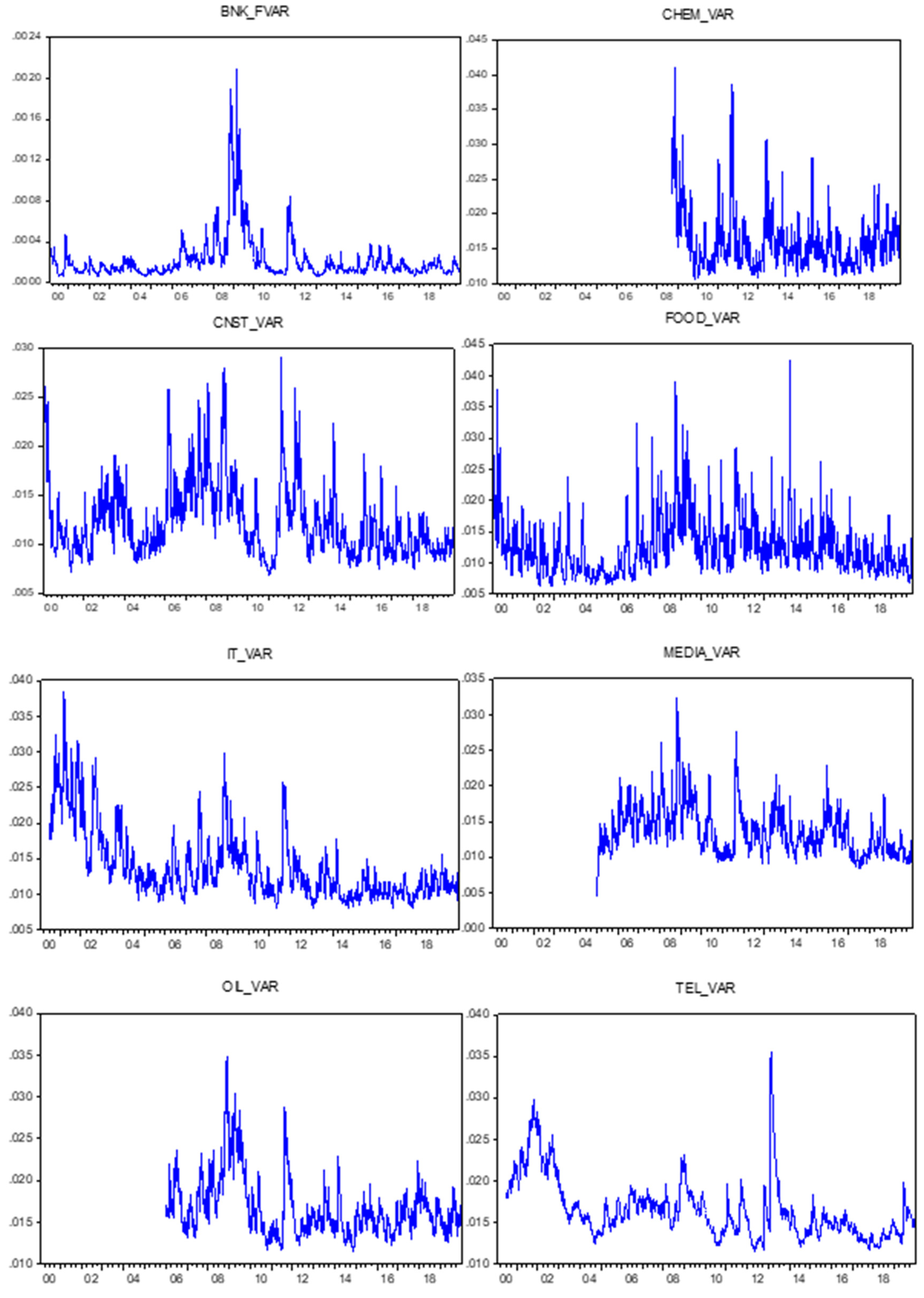
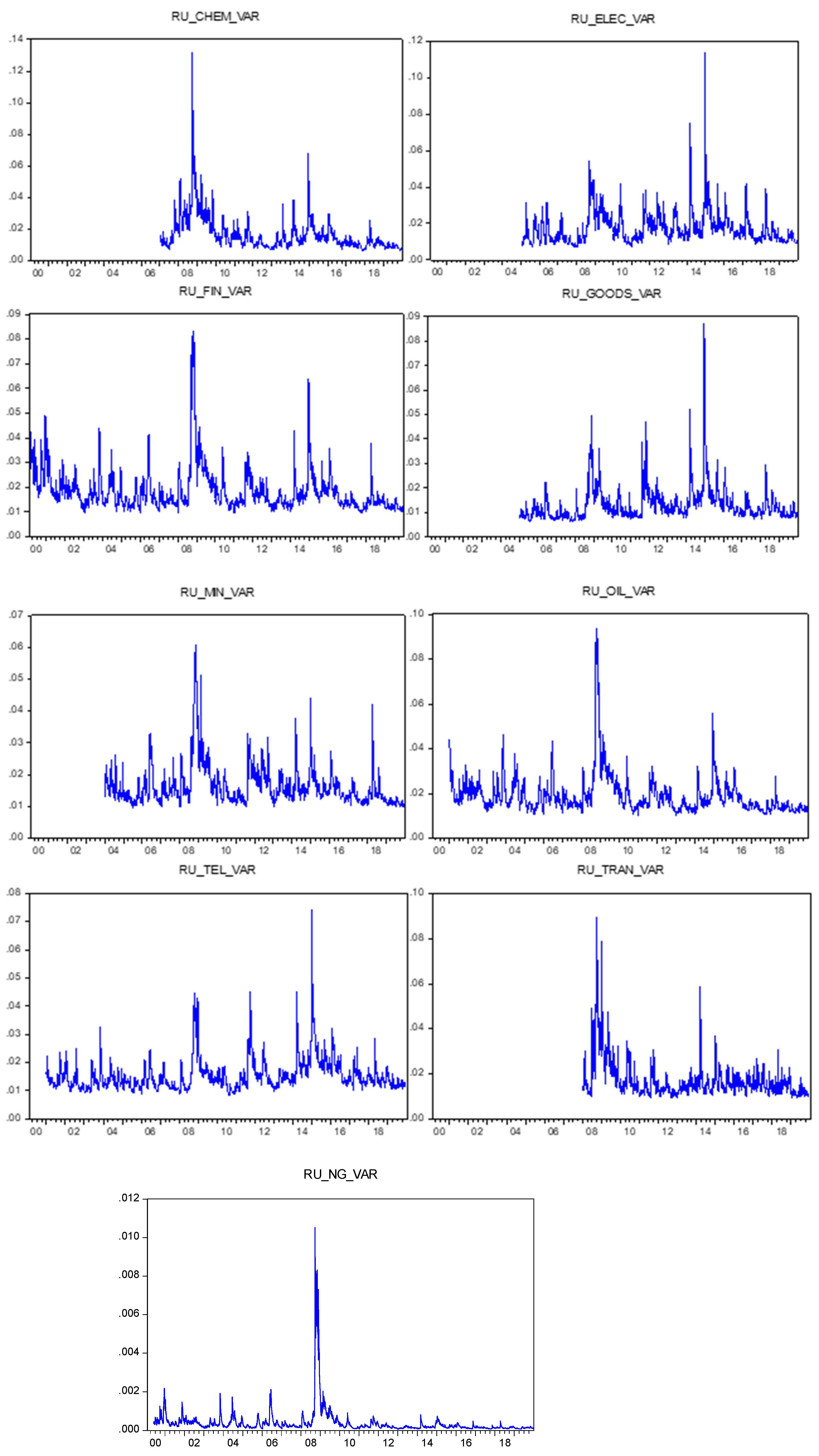
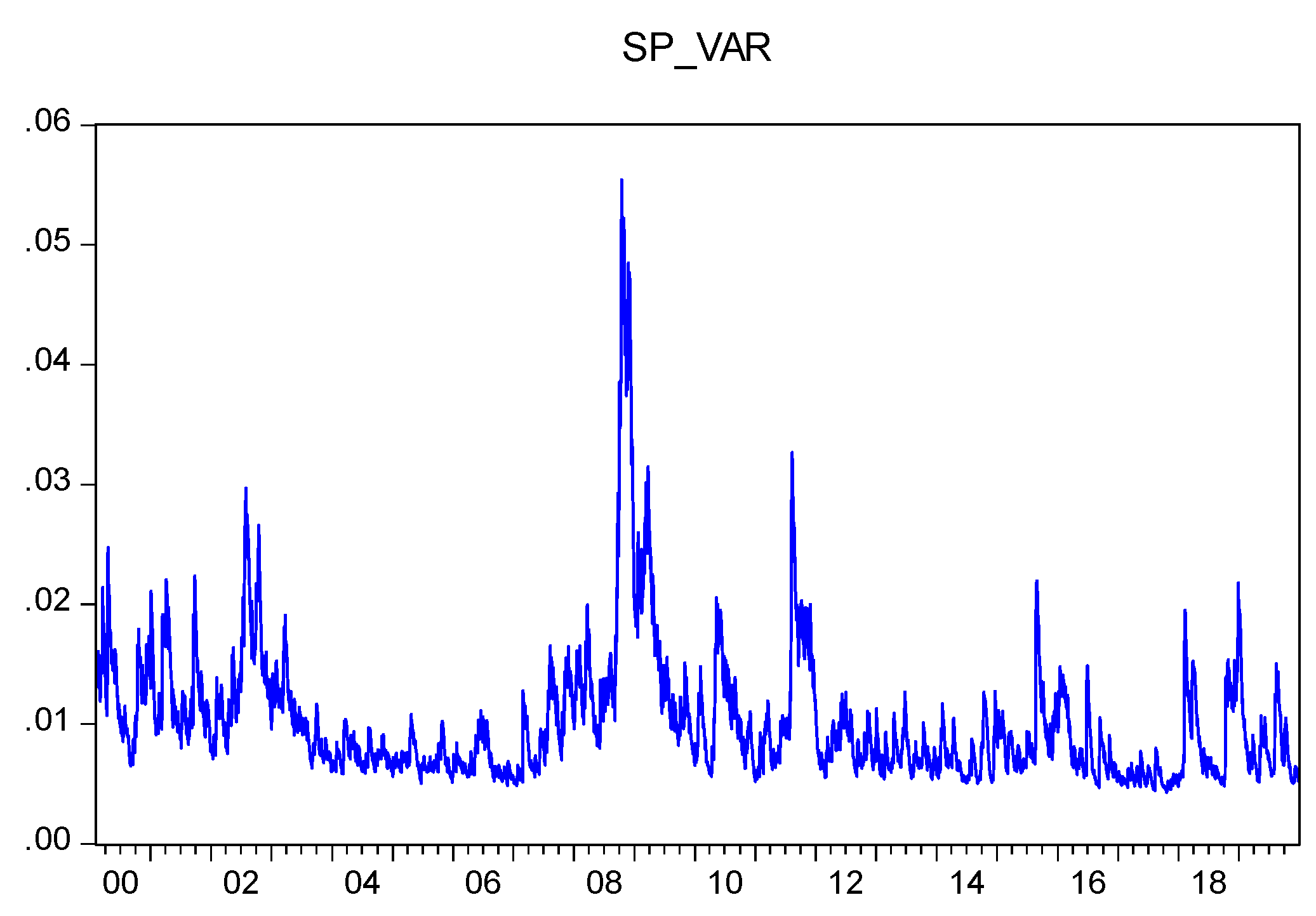
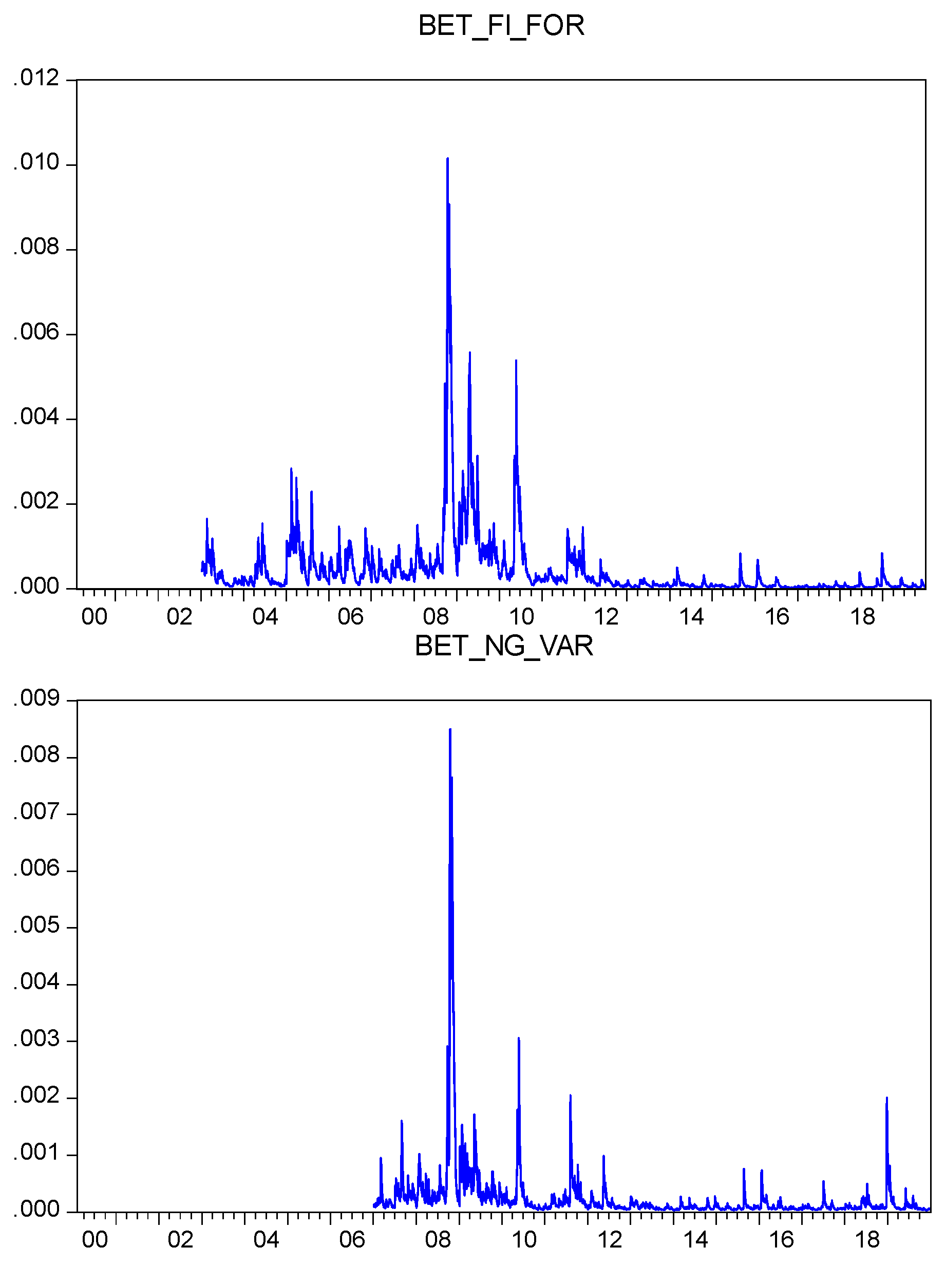
Appendix A presents the graphs of the volatility series used to determine the crisis period specific to each sector index (as seen in Table 1). They show an increased volatility for every index between 2008 and 2010, suggesting that all sectors have been affected by the GFC. However, the observed patterns are very different. Most sectors (the financial sector from all three countries, oil and gas from Poland and Russia, energy sector from Russia and Romania and chemical sector, mining and transport from Russia) registered the highest volatility during this timeframe, signaling that it was the one with the highest risk from the analyzed period. The other indices registered the highest volatility values outside the 2008–2010 period, suggesting that their evolution was influenced by other major events or, possibly, that the impact of the GFC was delayed by some factors. If they exist, they are of great importance at a sector level, even if they do not have national or global coverage.

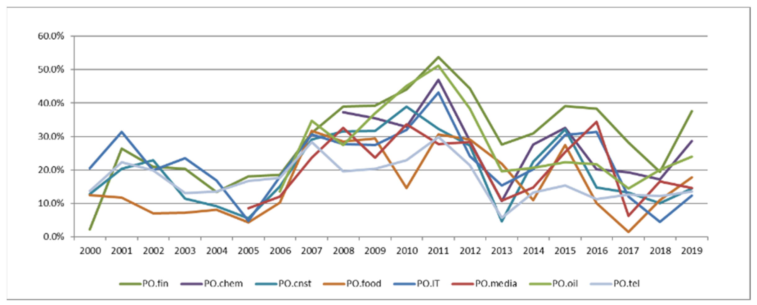
A basic analysis of the annual correlation coefficients between the sector indices and the S&P 500 index shows a high increase starting with the year 2007 or 2008, as seen in Figure 1, Figure 2 and Figure 3. This analysis can be considered a preliminary test, as it mostly conveys an increase in the interdependence between the analyzed indices with the S&P 500 index not necessarily a contagion (Pericoli and Sbracia 2003).

Figure 1 presents the evolution of the Polish sectors. As expected, the correlation level differs from one sector to the other. However, their annual evolution is similar to some extent: the coefficients show a high increase starting with 2007. The high level is maintained until the year 2011 or 2012, which is then followed by a significant decrease. Another increase, but with a lower magnitude, can be observed in 2015 or 2016, followed again by a substantial decrease. Moreover, as observed in Appendix B in

Table A1. Correlation coefficient for the Romanian sectors and Financial, Chemical and Construction sectors in Poland.

Correl. Coeff.	RO.Fin	RO.Energy	PO.Fin	PO.Chem	PO.Cnst
2000			2.2%		12.8%
2001			26.4%		20.4%
2002			21.0%		23.0%
2003	4.6%		20.3%		11.5%
2004	−5.1%		13.3%		9.2%
2005	−2.7%		18.1%		5.6%
2006	12.6%		18.6%		15.1%
2007	11.8%	3.5%	31.1%		29.1%
2008	29.6%	31.2%	38.9%	37.2%	31.6%
2009	31.7%	27.0%	39.2%	35.5%	31.7%
2010	31.7%	26.5%	44.1%	32.8%	38.9%
2011	32.0%	28.7%	53.7%	46.9%	32.4%
2012	26.4%	28.2%	44.4%	28.7%	27.3%
2013	15.9%	11.9%	27.6%	10.7%	4.6%
2014	19.0%	21.0%	30.9%	27.7%	22.5%
2015	31.6%	26.9%	39.0%	32.5%	32.2%
2016	31.9%	25.5%	38.3%	20.3%	14.8%
2017	13.3%	18.6%	28.2%	19.3%	13.2%
2018	3.7%	14.3%	19.5%	17.3%	10.1%
2019	12.7%	12.6%	37.6%	28.6%	14.5%
total	22.3%	25.3%	31.8%	30.1%	22.1%

Note: PO represents a sector index from the Warsaw Stock Exchange (Poland). RO represents a sector index from the Bucharest Stock Exchange (Romania). The table presents the annual correlation coefficients between the sector index and the S&P500 index. Values are depicted in bold if they are higher that the correlation coefficient between the sector index and the S&P500 index, determined for the whole analysis period. Missing values show that the sector index was not calculated in that specific year. Source: own calculation.

and

Table A2. Correlation coefficient for the remaining sectors in Poland.

Correl. Coeff.	PO.Food	PO.IT	PO.Media	PO.Oil	PO.Tel
2000	12.5%	20.5%			13.7%
2001	11.7%	31.4%			22.4%
2002	7.1%	19.9%			19.9%
2003	7.2%	23.6%			13.1%
2004	8.2%	16.8%			13.5%
2005	4.4%	4.8%	8.5%		16.8%
2006	10.2%	18.0%	12.1%	13.6%	17.7%
2007	31.7%	30.6%	23.7%	34.7%	28.3%
2008	28.5%	27.7%	32.6%	27.4%	19.6%
2009	29.4%	27.5%	23.7%	36.9%	20.4%
2010	14.5%	31.9%	33.6%	45.1%	23.0%
2011	30.6%	43.2%	27.8%	51.1%	29.9%
2012	29.2%	24.2%	28.3%	38.3%	21.4%
2013	21.9%	15.4%	10.9%	19.7%	5.7%
2014	10.9%	20.2%	14.8%	20.6%	13.3%
2015	27.4%	30.4%	25.4%	22.4%	15.3%
2016	10.1%	31.4%	34.4%	21.8%	11.3%
2017	1.5%	12.1%	6.3%	14.5%	12.7%
2018	11.0%	4.5%	16.6%	20.0%	12.3%
2019	17.8%	12.3%	14.6%	24.0%	13.5%
total	19.0%	23.9%	23.5%	29.1%	17.5%

Note: PO represents a sector index from the Warsaw Stock Exchange (Poland). The table presents the annual correlation coefficients between the sector index and the S&P500 index. Values are depicted in bold if they are higher that the correlation coefficient between the sector index and the S&P500 index, determined for the whole analysis period. Missing values show that the sector index was not calculated in that specific year. Source: own calculation.

, for most indices, the annual correlation is higher between 2007 and 2012 and 2015 and 2016 than the correlation coefficient determined for the whole analysis period. This is a signal that the link between the Polish economic sector and the US market was stronger during these periods. However, it does not show if this connection is observed during a crisis period, a recovery from the crisis period or during less turbulent, more optimistic times.

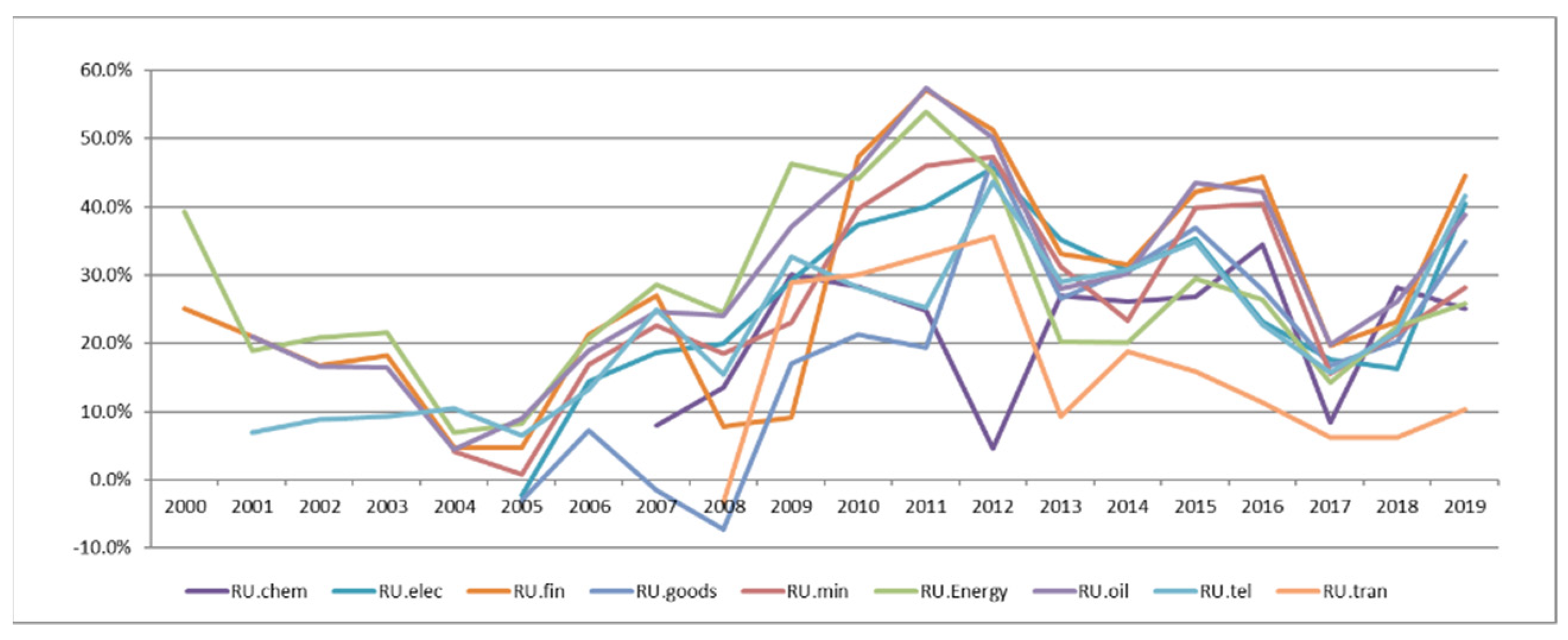
The evolution of the annual correlation between the Russian sector indices and the S&P 500 (Figure 2) shows that most indices record an increase in correlation in 2009. However, their situation is different from Poland because, with few exceptions, their level of correlation remains high until the end of the analysis period. The exceptions are 2013 and 2017 when most indices record an important decrease. This is also observed in Appendix B in

Table A3. Correlation coefficient for the chemical, electric utilities, financial, goods and mining sectors in Russia.

Correl. Coeff.	RU.Chem	RU.Elec	RU.Fin	RU.Goods	RU.Min
2000			25.0%
2001			21.0%
2002			16.7%
2003			18.2%
2004			4.7%		4.2%
2005		−2.2%	4.8%	−3.0%	0.8%
2006		14.4%	21.2%	7.2%	16.9%
2007	7.9%	18.7%	27.0%	−1.6%	22.6%
2008	13.6%	20.0%	7.9%	−7.3%	18.5%
2009	30.1%	29.2%	9.2%	17.1%	23.1%
2010	28.2%	37.4%	47.4%	21.3%	39.7%
2011	24.9%	40.0%	57.2%	19.3%	46.1%
2012	4.6%	45.7%	51.2%	47.2%	47.3%
2013	27.0%	35.2%	33.1%	26.5%	31.2%
2014	26.0%	30.7%	31.5%	30.8%	23.3%
2015	26.8%	35.4%	42.2%	36.9%	39.9%
2016	34.5%	23.1%	44.4%	27.8%	40.5%
2017	8.4%	17.6%	19.6%	16.7%	15.5%
2018	28.1%	16.4%	23.2%	20.2%	21.5%
2019	25.1%	40.5%	44.5%	34.8%	28.1%
total	20.3%	25.3%	22.4%	15.4%	25.5%

Note: RU represents a sector index from the Moscow Stock Exchange (Russia). The table presents the annual correlation coefficients between the sector index and the S&P500 index. Values are depicted in bold if they are higher that the correlation coefficient between the sector index and the S&P500 index, determined for the whole analysis period. Missing values show that the sector index was not calculated in that specific year. Source: own calculation.

and

Table A4. Correlation coefficient for the remaining sectors in Russia.

Correl. Coeff.	RU.Energy	RU.Oil	RU.Tel	RU.Tran
2000	39.2%
2001	18.9%	21.0%	7.0%
2002	20.8%	16.6%	8.8%
2003	21.6%	16.5%	9.3%
2004	7.0%	4.4%	10.4%
2005	8.3%	9.0%	6.5%
2006	20.7%	19.0%	13.3%
2007	28.6%	24.7%	24.9%
2008	24.5%	24.0%	15.4%	−3.3%
2009	46.4%	37.1%	32.7%	28.9%
2010	44.1%	45.6%	28.2%	30.0%
2011	53.9%	57.5%	25.2%	32.9%
2012	45.0%	50.2%	43.7%	35.7%
2013	20.2%	28.0%	29.0%	9.3%
2014	20.1%	30.2%	30.7%	18.9%
2015	29.5%	43.6%	34.8%	15.8%
2016	26.4%	42.2%	22.7%	11.3%
2017	14.3%	19.7%	15.7%	6.2%
2018	22.5%	26.2%	21.7%	6.2%
2019	25.9%	38.8%	41.6%	10.3%
total	27.7%	28.3%	19.8%	12.8%

Note: RU represents a sector index from the Moscow Stock Exchange (Russia). The table presents the annual correlation coefficients between the sector index and the S&P500 index. Values are depicted in bold if they are higher that the correlation coefficient between the sector index and the S&P500 index, determined for the whole analysis period. Missing values show that the sector index was not calculated in that specific year. Source: own calculation.

: between 2009 and 2019, in most cases, the annual correlation coefficients are higher than the one obtained for the whole analysis period. Furthermore, 2017 and 2018 offer the most cases of lower annual correlation. This suggests that the link between the national sector indices in Russia and the US market has changed after the beginning of the GFC.

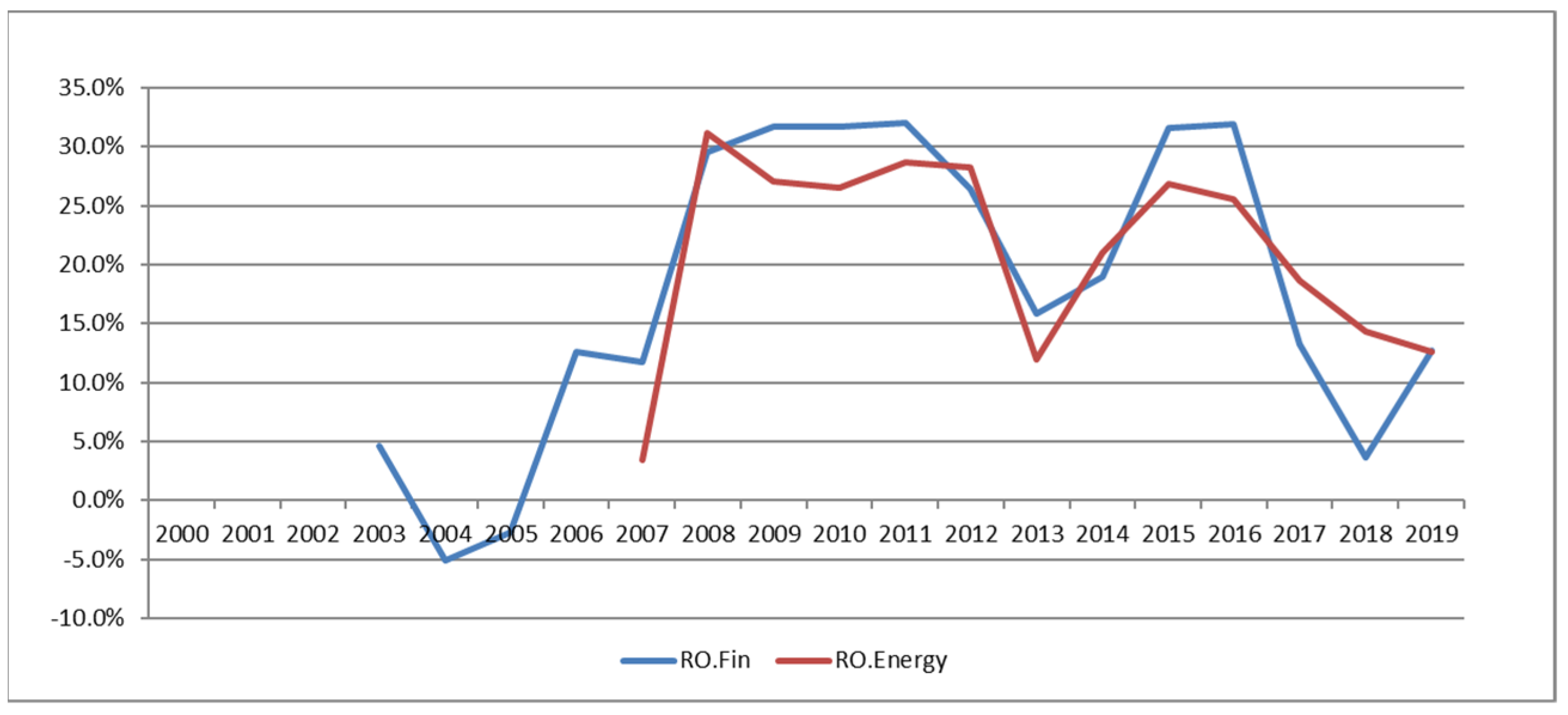
The analysis for the two Romanian sector indices (Figure 3) shows a significant increase of the annual correlation coefficient in 2008, followed by a period of relative stability until 2012. Then 2013 records an important decrease. In 2015 and 2016, the correlation levels jump to ones similar to 2009, followed again by a decrease. Additionally, the annual correlation coefficients between 2008 and 2012 and 2015 and 2016 are higher than the ones obtained for the whole period, as seen in Appendix B in Table A1. Thus, the situation of the Romanian indices is similar to the Polish ones.

These preliminary results point toward the fact that the 19 sector indices included in the analysis have been affected differently by the GFC. These results are in line with previous literature (e.g., Baur 2012; Chen et al. 2020; Țilică 2021). In order to better understand the pattern of this contagion process, the aforementioned methodology is employed and its results are presented in the following section.

5. Results

Table 2. DOW effect in the Polish sectors (1).

Coeff.	PO.Bank			PO.Chemicals			PO.Construction
	Dc1	Dc2	Ds	Dc1	Dc2	Ds	Dc1	Dc2	Ds
αi	0.06%	0.05%	0.05%	0.06%	0.06%	0.07%	−0.03%	−0.03%	−0.04%
αi,2	−0.04%	−0.03%	−0.03%	−0.06%	−0.06%	−0.07%	−0.02%	−0.02%	−0.02%
αi,3	−0.10% **	−0.10%	−0.09% *	−0.09%	−0.10%	−0.10%	0.00%	0.00%	0.01%
αi,4	−0.05%	−0.05%	−0.05%	−0.08%	−0.07%	−0.08%	0.04%	0.04%	0.04%
αi,5	−0.09% *	−0.10%	−0.10% *	0.04%	0.02%	0.03%	0.11% **	0.11% ***	0.11% ***
βi	33.22% ***	30.96% ***	29.58% ***	51.13% ***	47.37% ***	51.85% ***	29.14% ***	26.82% ***	29.72% ***
βi,2	−3.83%	1.08%	2.16%	−12.95%	−7.26%	−16.88% **	−8.40% *	−3.83%	−9.50% **
βi,3	−3.76%	−1.36%	−0.14%	−14.90% *	−11.97%	−15.51% **	−18.65% ***	−16.59% ***	−17.03% ***
βi,4	6.64%	6.75%	7.96%	−11.05%	−6.78%	−11.59%	−9.77% **	−9.86% **	−14.02% ***
βi,5	3.00%	6.19%	7.62%	−22.20% **	−18.55% **	−23.61% ***	−12.54% ***	−9.04% **	−11.61% ***
αi *	0.02%	0.41% *	0.72% ***	0.71% **	0.38%	0.11%	−0.30% *	−0.15%	0.28%
αi,2 *	0.05%	−0.42%	−0.80% **	−0.99% **	−0.42%	−0.56%	0.28%	0.19%	−0.12%
αi,3 *	0.00%	−0.49%	−0.84% **	−1.28% ***	−0.31%	−1.02%	0.29%	0.29%	−0.73%
αi,4 *	−0.35%	−0.51%	−0.65% *	−0.88% *	−0.47%	−1.80% *	−0.05%	0.04%	−1.19% *
αi,5 *	−0.25%	−0.59% *	−0.59%	−1.00% **	−0.03%	−1.78% *	0.06%	−0.21%	−1.63% **
βi *	9.52%	37.68% ***	50.10% ***	−8.39%	3.17%	−21.92%	5.03%	15.59% **	13.36%
βi,2 *	17.72%	−29.70% *	−38.35% **	−14.83%	−31.58% **	−1.13%	−6.25%	−26.85% **	−18.92%
βi,3 *	15.92%	−5.34%	−13.47%	4.45%	0.85%	19.45%	7.08%	−1.47%	−6.91%
βi,4 *	−42.56% ***	−52.68% ***	−64.17% ***	5.02%	−9.00%	−9.92%	−32.15% ***	−26.04% ***	−30.26% **
βi,5 *	6.21%	−24.50%	−41.54% **	−3.42%	−12.52%	46.73%	7.36%	−10.45%	−5.05%
LLH	15,410.92	15,406.87	15,412.98	8245.68	8245.42	8248.92	15,928.67	15,926.96	15,652.78

Note: PO represents a sector index from the Warsaw Stock Exchange (Poland). Dc1 represents the crisis dummy variable determined through the first assumption (August 2007 to March 2009), Dc2 is the one determined through the second analysis (9 June 2008–5 August 2009) and Ds is the crisis dummy variable specific to each sector index. ***, ** and * depict a 1%, 5% and 10% statistical significance, respectively. LLH stands for the Log likelihood indicator used to determine which of the three models is a better fit to the evolution of the sector index. Source: own calculation.

,

Table 3. DOW effect in the Polish sectors (2).

Coeff.	PO.Food			PO.IT			PO.Media
	Dc1	Dc2	Ds	Dc1	Dc2	Ds	Dc1	Dc2	Ds
αi	0.02%	0.00%	0.01%	0.07% **	0.07% ***	0.07% *	0.04%	0.03%	0.04%
αi,2	−0.01%	−0.01%	−0.01%	−0.09% *	−0.09% *	−0.09% *	−0.05%	−0.04%	−0.05%
αi,3	0.02%	0.03%	0.02%	−0.09% *	−0.09% *	−0.08% *	−0.01%	−0.01%	−0.01%
αi,4	0.00%	0.00%	−0.01%	−0.03%	−0.04%	−0.03%	−0.02%	−0.01%	−0.01%
αi,5	0.03%	0.03%	0.03%	0.01%	0.01%	0.01%	−0.01%	−0.02%	−0.02%
βi	14.02% ***	11.42% ***	14.85% ***	33.23% ***	29.25% ***	29.73% ***	38.51% ***	33.76% ***	35.52% ***
βi,2	−1.45%	2.05%	−2.58%	−6.64%	−3.19%	−4.29%	−6.20%	2.36%	−6.51%
βi,3	−5.36%	−2.54%	−4.25%	−10.26% *	−5.98%	−5.05%	−13.23% **	−9.28%	−12.62% **
βi,4	3.35%	3.80%	1.68%	−0.75%	−0.52%	−3.00%	−10.06%	−11.68% *	−15.60% ***
βi,5	−0.92%	1.88%	−0.90%	−4.50%	0.64%	−0.82%	−13.65% **	−6.14%	−6.89%
αi *	−0.30% **	0.13%	−0.45%	−0.20%	−0.03%	0.84%	0.00%	0.34% *	1.45% **
αi,2 *	−0.06%	−0.37%	0.46%	0.01%	−0.08%	−0.58%	−0.10%	−0.56% **	−1.55% *
αi,3 *	0.31% *	0.01%	0.11%	0.12%	0.18%	−2.38% *	−0.07%	−0.33%	−2.02% *
αi,4 *	0.01%	−0.09%	0.61%	0.03%	0.26%	−1.01%	−0.14%	−0.35%	−1.32%
αi,5 *	0.14%	−0.02%	0.04%	−0.13%	−0.23%	−1.94%	−0.13%	−0.36%	−2.67% ***
βi *	8.33%	20.94% ***	10.51%	−16.13% *	−2.40%	−10.92%	−8.84%	6.75%	0.74%
βi,2 *	−2.55%	−21.87% **	−12.16%	11.75%	−2.65%	1.39%	−3.87%	−35.05% ***	−14.21%
βi,3 *	4.32%	−9.63%	−6.50%	27.24% **	13.83%	5.36%	3.11%	−9.65%	3.56%
βi,4 *	−19.26% *	−13.41%	−17.71%	−12.31%	−8.04%	8.77%	−20.03% *	−12.20%	10.34%
βi,5 *	−5.49%	−22.39%	−7.25%	12.56%	−10.63%	5.34%	21.82%	−5.99%	−4.33%
LLH	15,931.72	15,928.64	15,660.27	15,082.45	15,073.77	15,075.64	11,529.65	11,529.00	11,529.16

Note: PO represents a sector index from the Warsaw Stock Exchange (Poland). Dc1 represents the crisis dummy variable determined through the first assumption (August 2007 to March 2009), Dc2 is the one determined through the second analysis (9 June 2008–5 August 2009) and Ds is the crisis dummy variable specific to each sector index. ***, ** and * depict a 1%, 5% and 10% statistical significance, respectively. LLH stands for the Log likelihood indicator used to determine which of the three models is a better fit to the evolution of the sector index. Source: own calculation.

,

Table 4. DOW effect in the Polish and Russian sectors.

Coeff.	PO.Oil and Gas			PO.Telecommunication			RU.Chemicals
	Dc1	Dc2	Ds	Dc1	Dc2	Ds	Dc1	Dc2	Ds
αi	0.16% ***	0.15% ***	0.15% ***	0.07% *	0.08% **	0.08% **	0.04%	0.04%	0.04%
αi,2	−0.14% *	−0.12%	−0.12%	−0.06%	−0.08%	−0.07%	−0.09%	−0.09%	−0.09%
αi,3	−0.14% *	−0.10%	−0.10%	−0.15% **	−0.17% ***	−0.16% ***	−0.03%	−0.03%	−0.03%
αi,4	−0.25% ***	−0.26% ***	−0.25% ***	−0.08%	−0.10%	−0.09%	−0.02%	−0.01%	−0.01%
αi,5	−0.19% **	−0.19% **	−0.20% **	−0.07%	−0.08%	−0.09%	−0.07%	−0.06%	−0.06%
βi	63.04% ***	56.00% ***	52.26% ***	38.46% ***	37.42% ***	33.84% ***	26.96% ***	22.41% ***	24.53% ***
βi,2	−10.68%	−3.51%	−0.99%	−14.06	−12.32% **	−12.77% ***	−1.62%	3.21%	0.45%
βi,3	−16.72% **	−11.70%	−9.83%	−17.46% ***	−15.36% **	−13.66% **	−1.67%	3.44%	1.28%
βi,4	−3.12%	−4.06%	−3.83%	−15.34% **	−14.68% **	−13.61% ***	2.25%	5.74%	4.21%
βi,5	−17.75% **	−9.06%	−5.44%	−10.10% *	−8.71%	−4.38%	2.68%	6.37%	4.24%
αi *	−0.30%	0.06%	0.24%	0.19%	0.04%	0.97%	0.12%	0.25%	0.90%
αi,2 *	0.36%	−0.18%	−0.19%	−0.18%	0.19%	0.17%	−0.17%	−0.23%	−0.89%
αi,3 *	0.64% **	−0.09%	−0.27%	−0.37%	−0.06%	−2.14% *	0.14%	−0.24%	−1.04%
αi,4 *	0.05%	0.61% *	0.16%	−0.32%	0.04%	−0.97%	−0.01%	−0.35%	−0.64%
αi,5 *	−0.09%	−0.50%	−0.49%	−0.21%	−0.31%	−0.94%	0.22%	−0.16%	−1.15%
βi *	−37.18% ***	−16.75%	−9.36%	−17.78% **	−13.36%	0.88%	7.33%	45.73% ***	42.52% *
βi,2 *	19.12%	−7.19%	−19.90%	1.96%	−13.68%	−34.26%	−9.31%	−56.26% **	−40.86%
βi,3 *	23.81%	8.44%	11.46%	6.70%	−5.17%	−35.22%	9.09%	−31.37%	−22.82%
βi,4 *	−10.29%	0.36%	4.64%	−4.40%	−8.64%	−12.10%	−21.78%	−56.77% **	−59.58% *
βi,5 *	50.83% ***	34.60% *	31.70%	21.06%	17.48%	−14.62%	−19.76%	−65.45% *	−72.61% *
LLH	10,080.21	10,069.48	10,065.75	14,226.42	14,227.51	14,225.16	9753.07	9757.93	9754.779

Note: PO represents a sector index from the Warsaw Stock Exchange (Poland). RU depicts an index from the Moscow Stock Exchange (Russia). Dc1 represents the crisis dummy variable determined through the first assumption (August 2007 to March 2009), Dc2 is the one determined through the second analysis (9 June 2008–5 August 2009) and Ds is the crisis dummy variable specific to each sector index. ***, ** and * depict a 1%, 5% and 10% statistical significance, respectively. LLH stands for the Log likelihood indicator used to determine which of the three models is a better fit to the evolution of the sector index. Source: own calculation.

,

Table 5. DOW effect in the Russian sectors.

Coeff.	RU.Electric Utilities			RU.Financials			RU.Goods
	Dc1	Dc2	Ds	Dc1	Dc2	Ds	Dc1	Dc2	Ds
αi	0.12% **	0.10% **	0.10% **	0.15% ***	0.15% ***	0.15% ***	0.10% ***	0.08% ***	0.08% **
αi,2	−0.15% **	−0.15% **	−0.15% ***	−0.13% **	−0.13% **	−0.14% **	−0.03%	−0.03%	−0.04%
αi,3	−0.06%	−0.08%	−0.06%	−0.10% *	−0.09%	−0.08%	−0.02%	−0.02%	−0.01%
αi,4	−0.09%	−0.06%	−0.05%	−0.04%	−0.04%	−0.04%	0.01%	0.03%	0.03%
αi,5	−0.06%	−0.03%	−0.02%	−0.09%	−0.07%	−0.08%	−0.08% *	−0.05%	−0.06%
βi	33.33% ***	24.93% ***	26.92% ***	40.66% ***	39.39% ***	39.40% ***	26.21% ***	23.32% ***	20.65% ***
βi,2	6.56%	2.48%	0.28%	2.73%	1.01%	0.56%	−8.31%	−13.91% **	−12.88% **
βi,3	−2.17%	−1.35%	−4.87%	1.61%	1.40%	−0.63%	−12.28% **	−12.14% **	−11.92% **
βi,4	12.83% *	8.39%	4.99%	15.70% **	13.01% **	12.74% **	−0.53%	−2.41%	−1.07%
βi,5	9.75%	7.51%	3.57%	14.18% **	11.98% *	11.19% *	−5.88%	−13.93% **	−10.94% **
αi *	−0.15%	−0.16%	1.00%	−0.04%	−0.23%	−0.27%	−0.15%	−0.04%	0.35%
αi,2 *	0.08%	−0.32%	−2.95% ***	−0.14%	−0.46%	0.27%	−0.03%	−0.37% *	−0.12%
αi,3 *	−0.06%	0.49%	−1.90%	0.23%	0.43%	−0.48%	0.06%	0.10%	0.32%
αi,4 *	0.10%	0.27%	−1.36%	−0.07%	0.17%	0.66%	0.12%	−0.06%	0.03%
αi,5 *	0.23%	0.18%	−1.23%	0.23%	−0.22%	0.21%	0.12%	−0.16%	−0.30%
βi *	−17.81% *	17.56% *	34.12% **	−16.34%	−13.58%	−17.13%	−17.33% **	−11.38%	0.86%
βi,2 *	−22.24% *	−34.01% **	−53.84% *	−10.98%	−31.85%	−34.60%	−7.42%	−2.62%	4.08%
βi,3 *	−8.05%	−26.64%	−42.63%	−10.83%	−25.37%	−9.30%	1.07%	−8.84%	−1.15%
βi,4 *	−22.63% *	−21.99%	−23.74%	−51.78% ***	−52.88% **	−105.72% ***	−2.80%	−2.10%	−11.81%
βi,5 *	−16.87%	−49.58% ***	−27.80%	−6.88%	−7.26%	31.46%	−6.14%	13.18%	−3.95%
LLH	11,046.78	11,015.56	11,014.68	14,130.73	14,124.73	14,124.28	12,103.40	12,085.28	12,079.69

Note: RU depicts an index from the Moscow Stock Exchange (Russia). Dc1 represents the crisis dummy variable determined through the first assumption (August 2007 to March 2009), Dc2 is the one determined through the second analysis (9 June 2008–5 August 2009) and Ds is the crisis dummy variable specific to each sector index. ***, ** and * depict a 1%, 5% and 10% statistical significance, respectively. LLH stands for the Log likelihood indicator used to determine which of the three models is a better fit to the evolution of the sector index. Source: own calculation.

,

Table 6. DOW effect in the Russian sectors (2).

Coeff.	RU.Mining			RU.Oil and Gas			RU.Telecommunication
	Dc1	Dc2	Ds	Dc1	Dc2	Ds	Dc1	Dc2	Ds
αi	0.08% *	0.07%	0.07%	0.15% ***	0.15% ***	0.15% ***	0.12% ***	0.12% ***	0.12% ***
αi,2	−0.02%	−0.01%	−0.02%	−0.16% **	−0.16% **	−0.16% ***	−0.05%	−0.06%	−0.07%
αi,3	−0.02%	0.02%	0.02%	−0.14% **	−0.13% **	−0.12% **	−0.09% *	−0.08% *	−0.08% *
αi,4	0.00%	0.01%	0.02%	−0.07%	−0.07%	−0.06%	−0.04%	−0.04%	−0.03%
αi,5	−0.06%	−0.03%	−0.02%	−0.08%	−0.08%	−0.08%	−0.04%	−0.03%	−0.04%
βi	36.16% ***	35.44% ***	36.38% ***	47.86% ***	44.05% ***	45.30% ***	21.07% ***	18.73% ***	21.38% ***
βi,2	−5.19%	−8.94%	−11.65% *	−3.86%	−1.73%	−4.20%	−5.79%	−4.32%	−7.19%
βi,3	−1.00%	−1.64%	−2.89%	0.10%	1.26%	−0.78%	−8.21%	−5.93%	−8.34% *
βi,4	13.21% *	10.02%	8.59%	12.31% *	11.98% *	10.53%	5.66%	6.18%	2.86%
βi,5	10.30%	7.58%	5.70%	9.07%	10.05%	7.74%	3.39%	2.91%	0.38%
αi *	−0.18%	0.10%	0.84%	0.02%	0.04%	0.07%	−0.01%	0.12%	−0.14%
αi,2 *	−0.12%	−0.86% **	−1.86% ***	−0.04%	−0.62%	−0.21%	−0.25%	−0.61% ***	−0.79%
αi,3 *	0.52% **	−0.10%	−1.69% **	0.23%	0.07%	0.03%	0.04%	−0.02%	−0.06%
αi,4 *	0.27%	0.36%	−0.69%	−0.02%	0.06%	−0.02%	0.01%	0.02%	−0.60%
αi,5 *	0.35%	−0.24%	−1.39% **	0.03%	−0.28%	0.05%	0.02%	−0.30%	−0.44%
βi *	−4.08%	4.30%	7.16%	2.40%	38.46% **	32.25%	4.58%	18.06% **	4.58%
βi,2 *	−22.87%	−26.52%	−6.54%	−18.80%	−66.81% ***	−33.84%	−9.96%	−24.82% **	−12.86%
βi,3 *	−10.77%	−18.55%	−27.48%	−21.70%	−41.66% *	−9.03%	−2.94%	−17.08%	−3.31%
βi,4 *	−32.43% *	−14.39%	−10.36%	−46.76% **	−49.70% **	−47.74%	−25.23% **	−34.07% ***	−36.76%
βi,5 *	−23.62%	−47.37% *	−51.54%	−26.81%	−71.63%	−33.35%	−18.71%	−24.54%	−13.44%
LLH	11,858.15	11,851.2	11,849.86	13,330.01	13,327.36	13,323.99	14,441.86	14,441.95	14,439.71

Note: RU depicts an index from the Moscow Stock Exchange (Russia). Dc1 represents the crisis dummy variable determined through the first assumption (August 2007 to March 2009), Dc2 is the one determined through the second analysis (9 June 2008–5 August 2009) and Ds is the crisis dummy variable specific to each sector index. ***, ** and * depict a 1%, 5% and 10% statistical significance, respectively. LLH stands for the Log likelihood indicator used to determine which of the three models is a better fit to the evolution of the sector index. Source: own calculation.

,

Table 7. DOW effect in the Russian energy sector (3).

Coeff.	RU.Transport			RU.Energy
	Dc1	Dc2	Ds	Dc1	Dc2	Ds
αi	−0.02%	−0.04%	−0.04%	0.11% ***	0.11% ***	0.11% ***
αi,2	−0.01%	0.01%	0.01%	−0.08%	−0.08%	−0.08%
αi,3	0.07%	0.08%	0.09%	−0.10% *	−0.10% *	−0.09% *
αi,4	−0.01%	0.00%	0.00%	−0.10% *	−0.10% *	−0.10% *
αi,5	−0.01%	−0.02%	−0.01%	−0.03%	−0.03%	−0.03%
βi	28.94% ***	24.31% ***	26.88% ***	45.82% ***	41.95% ***	41.42% ***
βi,2	−9.24%	0.53%	−2.56%	−10.31% *	−5.99%	−6.23%
βi,3	−8.03%	−3.79%	−6.14%	−3.49%	−1.09%	−1.06%
βi,4	0.54%	0.62%	−1.01%	1.41%	1.92%	2.29%
βi,5	−7.25%	0.29%	−3.49%	−7.59%	−3.93%	−4.03%
αi *	−0.29%	0.22%	0.70% *	0.14%	0.21%	0.24%
αi,2 *	0.21%	−0.80% **	−1.25% **	−0.28%	−0.78% *	−0.43%
αi,3 *	0.26%	−0.02%	−0.76%	0.11%	0.12%	−0.09%
αi,4 *	0.08%	−0.48%	−0.67%	−0.23%	−0.05%	0.11%
αi,5 *	−0.06%	0.03%	−0.14%	−0.06%	−0.45%	0.09%
βi *	4.51%	49.76% ***	37.87% ***	12.76%	65.91% ***	73.99% ***
βi,2 *	−2.56%	−88.15% ***	−78.38% ***	−12.47%	−75.08% ***	−68.25% ***
βi,3 *	−5.62%	−47.26% **	−40.19%	−15.73%	−43.55% *	−28.05%
βi,4 *	−25.04%	−45.93% ***	−37.75% *	−48.22% **	−59.83% ***	−62.61% ***
βi,5 *	−4.44%	−82.29% ***	−65.68% **	−13.42%	−68.63% **	−50.67%
LLH	8814.45	8820.24	8816.18	14,247.67	14,252.58	14,255.01

Note: RU depicts an index from the Moscow Stock Exchange (Russia). Dc1 represents the crisis dummy variable determined through the first assumption (August 2007 to March 2009), Dc2 is the one determined through the second analysis (9 June 2008–5 August 2009) and Ds is the crisis dummy variable specific to each sector index. ***, ** and * depict a 1%, 5% and 10% statistical significance, respectively. LLH stands for the Log likelihood indicator used to determine which of the three models is a better fit to the evolution of the sector index. Source: own calculation.

and

Table 8. DOW effect in the Romanian energy and financial sectors.

Coeff.	RO.Financial			RO.Energy
	Dc1	Dc2	Ds	Dc1	Dc2	Ds
αi	−0.06% *	−0.06% *	−0.06% **	−0.02%	−0.02%	−0.02%
αi,2	0.03%	0.03%	0.03%	0.03%	0.03%	0.03%
αi,3	0.07% *	0.06% *	0.06% *	0.01%	0.02%	0.01%
αi,4	0.08% **	0.08% **	0.07% *	0.07%	0.07%	0.07%
αi,5	0.13% ***	0.13% ***	0.13% ***	0.08% *	0.09% **	0.09% **
βi	16.89% ***	15.92% ***	16.53% ***	33.22% ***	31.50% ***	32.50% ***
βi,2	−7.01%	−6.18%	−6.27%	−22.03% ***	−19.65% ***	−20.46% ***
βi,3	−3.56%	−1.94%	−2.56%	−16.72% ***	−15.69% ***	−17.04% ***
βi,4	3.05%	3.37%	2.98%	−19.35% ***	−19.37% ***	−20.68% ***
βi,5	2.37%	3.84%	3.27%	−15.76% ***	−14.07% ***	−14.71% ***
αi *	−0.17%	0.05%	0.30%	−0.11%	0.30%	0.49%
αi,2 *	−0.18%	−1.09% ***	−0.72%	−0.25%	−0.85% ***	−1.25% ***
αi,3 *	−0.46% *	−0.48%	−1.20% *	−0.16%	−0.43%	−0.26%
αi,4 *	−0.48% *	−0.47%	−0.39%	−0.37%	−0.22%	−0.07%
αi,5 *	0.06%	−0.20%	−0.68%	−0.03%	−0.63% *	−0.52%
βi *	14.55%	44.61% ***	28.74% **	−9.77%	7.83%	0.82%
βi,2 *	−0.19%	4.95%	−8.96%	24.55% *	8.75%	20.52%
βi,3 *	13.83%	−14.32%	6.49%	0.03%	−3.17%	14.09%
βi,4 *	−31.48% *	−40.09% *	−32.17%	−5.99%	4.59%	22.01%
βi,5 *	−0.19%	−24.46%	−8.90%	10.82%	−1.02%	−3.28%
LLH	13,053.17	13,052.21	13,048.77	10,669.66	10,667.12	10,668.08

Note: RO suggests an index from the Bucharest Stock Exchange (Romania). Dc1 represents the crisis dummy variable determined through the first assumption (August 2007 to March 2009), Dc2 is the one determined through the second analysis (9 June 2008–5 August 2009) and Ds is the crisis dummy variable specific to each sector index. ***, ** and * depict a 1%, 5% and 10% statistical significance, respectively. LLH stands for the Log likelihood indicator used to determine which of the three models is a better fit to the evolution of the sector index. Source: own calculation.

present the results obtained for the 19 sector indices by using, consecutively, the three possible definitions of the crisis period. For most indices, the model with the best fit (with higher values of LLH) is represented by the one which uses the crisis dummy variable that takes into account the period of time when negative news announcements were made on the US market (Dc1). Some sectors exhibit a different behavior. The telecommunication sectors from both Poland and Russia and the chemicals and transportation sectors from Russia are best described by Dc2 (the period of high US market volatility). The banking and chemicals sectors from Poland and the energy sector from Russia show a better fit for the model with Ds which includes the crisis period specific to each sector index. The following comments regarding the pattern observed for each of the 19 indices are based on the results obtained on the model with the better fit. However, these patterns do not differ significantly from the ones obtained for the other two crisis definitions which suggests the robustness of the findings.

Table 2 presents the results for the banking, chemicals and construction sectors from Poland. The first sector had a very strong, stable connection with the US market in non-crisis periods (β_i is positive and statistically significant and the rest are not significant). During the crisis period, the link increases and it becomes more calendar variant: higher connection on Mondays than on Tuesdays, Thursdays and Fridays. The evolutions of the chemical and construction sectors are very different during the non-crisis periods: the spillovers from the US market were dependent on the day of the week: higher on Mondays than the other weekdays (β_i is positive and statistically significant and the rest are negative). During the GFC, this connection appears to remain the same (all β_i* coefficients are not significant), suggesting that the US financial turmoil has not determined new effects on these sectors.

Table 3 shows the results for the food, IT and media Polish sectors. During the non-crisis periods, the DOW effect was not present on the food sector, but it influenced both the national evolution of the IT index and the US spillovers to this sector, leading to a lower connection on Wednesdays (β_i and β_i,3 are statistically significant). During the crisis period, the spillovers from the US market continued throughout the week and even increased on Wednesdays (β_i* + β_i,3* is positive) in the IT sector, but they seem to maintain the same pattern in the food sector. The oil and gas index, as seen in Table 4, showed a similar pattern to the IT sector, with the distinction that the increased connection happened on Fridays during the GFC. The media and telecommunication indices show little sign of financial contagion. However, during the non-crisis period, their connection to the US market is stronger on Mondays than the other weekdays. Additionally, the oil and gas sectors, alongside the banking system, appear to be the ones which were the most affected by the GFC, by registering the highest positive coefficients (50.10% on Mondays for the latter and 50.83% on Fridays for the former).

The study of the Russian market (MSE) begins in Table 4 with the chemicals sector, while Table 5 presents the electric utilities, financials and consumer goods. Similar to the ones from WSE, they show a strong connection to the US market during non-crisis periods which is affected by the DOW effect, with the exception of the chemicals sector. However, while the electric utilities and financial sector appear to have a stronger link towards the end of the week (positive coefficients), the consumer goods sector registers the highest relation on Mondays. During the GFC period, the otherwise stable connection of the chemical sector to the US market changes, becoming affected by the DOW effect. For the other three sectors, the spillovers from the US market seem to decrease (β_i* coefficients are negative).

The last analyzed indices from the MSE are presented in Table 6 and Table 7. The strong connection with the US market is also observed for each of them during the non-crisis period. However, the calendar pattern is observed only for two sectors: mining and oil and gas which register higher spillovers on Thursday. For these indices, during the crisis period, the connection decreases significantly on Thursdays, leading to negative parameters. The other three sectors, telecommunication, transport and energy, show an increase of the link during Mondays (suggesting the existence of financial contagion) and subsequent decreases in other weekdays, which can be linked to the DOW effect. Additionally, the energy sector is the one which appears to be the most affected by the GFC, when compared to other Russian sectors, by registering the highest coefficient on Mondays (73.99%).

Romania is the final market taken into consideration in this analysis. The results obtained for its two sector indices, presented in Table 8, show that their evolution is very different. During the non-crisis period, the national evolution of the financial index was affected by the DOW effect and it showed a stable and strong connection with the US market. The same strong link can be seen in the energy sector, but it appears to be affected by the calendar pattern, leading to stronger ties on Mondays than the rest of the weekdays. During the GFC, the US spillovers to the financial sector remain the same most days, with the exception of Thursdays when they seem to decrease. However, the energy sector appears to experience an increased connection to the US market on Tuesdays. This suggests that the financial contagion process can be observed and that it is affected by the DOW effect.

6. Discussion

Table 9. Results obtained for the 19 sector indices.

Sector Index	DOW, Non-Crisis Period		DOW, Crisis Period		Best Fit Model
	National	US Market	National	US Market
PO.bank	Y	Poz(1)	Y	Y+	Ds
PO.chemicals	NS	Y	Y	NS	Ds
PO.construction	Y	Y	Y	Neg(4)	Dc1
PO.food	NS	Poz(1)	Y	Neg(4)	Dc1
PO.IT	Y	Y	NS	Y-(3)	Dc1
PO.media	NS	Y	NS	Neg(4)	Dc1
PO.oil and gas	Y	Y	Y	Y-(5)	Dc1
PO.telecommunication	Y	Y	NS	NS	Dc2
RU.chemicals	NS	Poz(1)	NS	Y+	Dc2
RU.electric utilities	Y	Y	NS	Neg(1,2,4)	Dc1
RU.financials	Y	Y	NS	Neg(4)	Dc1
RU.goods	Y	Y	NS	Neg(1)	Dc1
RU.mining	NS	Y	Y	Neg(4)	Dc1
RU.oil and gas	Y	Y	NS	Neg(4)	Dc1
RU.telecommunication	Y	Poz(1)	Y	Y+	Dc2
RU.transport	NS	Poz(1)	Y	Y+	Dc2
RU.Energy	Y	Poz(1)	NS	Y+	Ds
RO.financial	Y	Poz(1)	Y	Neg(4)	Dc1
RO.energy	Y	Y	NS	Y-(2)	Dc1

Note: DOW represents the day of the week effect, national refers to the evolution of the national-specific, sector index (alpha coefficients for crisis and non-crisis periods), US market to the link between the sector index and the S&P500 index (beta coefficients for crisis and non-crisis periods). PO stands for an index from the Warsaw Stock Exchange (Poland), RU depicts an index from the Moscow Stock Exchange (Russia) and RO suggests an index from the Bucharest Stock Exchange (Romania). Best fit model includes the crisis definition that best describes the index evolution, based on the log likelihood indicator. Dc1 represents the crisis dummy variable determined through the first assumption (August 2007 to March 2009), Dc2 is the one determined through the second analysis (9 June 2008–5 August 2009) and Ds is the crisis dummy variable specific to each sector index. Y means that the results showed the presence of the DOW effect, NS means that the obtained coefficients are not significant (no DOW effect), Poz(1) means that spillovers from the US market are present, but do not vary during weekdays. Y+ shows that contagion was present during the GFC, Monday’s spillovers being higher than in other weekdays. Y- shows that contagion was present during the GFC, but non-Monday spillovers during crisis periods are lower. Neg shows that contagion is not observed, but the link with the US market appears to decrease in certain weekdays. The value in brackets represents the weekdays that registered a significant coefficient. Source: own calculation.

presents an overview of the findings obtained for the 19 sector indices from the three East European countries. The results included in the table are the ones which recorded the highest LLH indicator, signaling the model with the best fit.

Furthermore, 12 of these indices have the best fit when using as crisis definition the period when negative announcements were visible on the US market (Dc1), suggesting that these sectors are highly connected to the American newsfeed. This result is in line with existing literature that shows the important impact that news announcements have on the evolution of stock markets (e.g., Kim et al. 2019; Cepoi 2020). The telecommunication sectors from Poland and Russia as well as the chemicals and transport sectors in Russia seem to have been in crisis during the high volatility period of the US market (Dc2). The only ones that were best defined by the period when the specific sector registered high volatility are the financial and chemicals sectors in Poland and the energy sector in Russia. These findings signal that, even though all sectors were affected by the crisis, the timeframe when they were affected is different. Thus, investors that seek to diversify their international portfolios, including during turbulent times, may benefit from these results: they suggest that the moment to enter and/or exit a specific sector is different, thus supporting the diversification process.

The results show that all the analyzed indices exhibit the presence of the DOW effect in their evolution during non-crisis and/or turbulent periods. This finding supports existing literature that showed that East European markets are highly susceptible to these calendar anomalies (e.g., Guidi et al. 2011; Oprea and Țilică 2014). An important contribution of this paper is showing that these patterns are not typical for a certain market, with sectors from the same market developing different variations of the DOW effect. This anomaly’s presence can provide useful insights to academics, especially the ones concerned with market efficiency, as it signals the low level of efficiency for these sectors (Dragotă and Țilică 2014).

Spillovers from the US market to all the analyzed indices can be observed during crisis and/or non-crisis periods. This highlights the strong connection between these sectors and the international market. However, an increase in comovements during the GFC can be observed for only eight sectors: financial, IT and oil and gas from Poland, chemicals, telecommunications, transport and energy from Russia and energy from Romania. This highlights that the contagion process has affected differently the economic sectors, which is in line with previous literature (e.g., Baur 2012; Țilică 2021).

An interesting fact is represented by the significant negative coefficient registered by nine of the analyzed sectors regarding the spillovers from the US market during the crisis period. Most of them, with the exception of the Russian commercial goods sector, are obtained for the fourth weekday. This is not a typical sign of contagion, as it does not show an increase of comovements but a decrease. However, it could signal that an important factor influences the connection between these sectors and the US market. Future research could be developed in this direction, endeavoring to discover and explain the nature of this factor.

The main purpose of this paper is to determine if the DOW effect can be observed in the financial contagion process that affected the sectors during the GFC. Contagion can be observed in eight of the studied indices and, for all of them, a calendar variant pattern is present. Five of the eight sectors show that, during the crisis period, the Monday spillovers are higher than the ones from the rest of the weekdays (financial sector in Poland and chemicals, telecommunication, transport and energy in Russia). The other three show that spillovers in another weekday during the GFC are higher: Wednesday for the Polish IT sector, Friday for the Polish oil and gas sector and Tuesday for the Romanian energy sector. These results are similar to the ones obtained by Sewraj et al. (2019) when investigating different developed West European markets.

These findings represent the main contribution of the paper, obtained by employing a novel approach that takes into account both the perspectives of Baur (2012) and Sewraj et al. (2019). They suggest that investors interested in international portfolio diversification, including in turbulent times, are not obligated to completely exit the Eastern European markets. Instead, by performing intra-weekly trades, they could enter certain sectors in the days when contagion risk is minimal. Further research should be performed to ascertain the profitability of such strategies, by also taking into account the impact of the trading fees (which can be significant given a high number of trades).

7. Conclusions

Academic literature has been focused on analyzing financial contagion, presumably as it studies a common event from real life: the shocks’ transmission from one country (or market) to another. The presence of shocks in capital markets is a usual occurrence that can be caused by various aspects (e.g., financial, healthcare, macroeconomic). The important technological improvements from the last decades (both in terms of digitalization and globalization) have led to a higher connection between the capital markets and the economic sectors of different countries. Thus, a shock from a certain financial environment will, most likely, be transmitted to other countries. For this reason, financial literature has been constantly studying their transmission process, both during historical events (e.g., the 1987 crash) and current ones (e.g., the COVID-19 crisis).

This paper investigates the presence of the DOW effect in financial contagion during the GFC. The analysis is conducted on several economic sectors from three Post-Communist East European markets: Poland, Romania and Russia. The three were chosen as they are the only ones from this region that provide national-specific sector indices. The database consists in their daily returns for the period 1 January 2000–30 December 2019. This leads to a total number of 19 indices (8 from Poland, 2 from Romania and 9 from Russia). The methodological approach consists in a GJR-GARCH framework applied in a model that includes dummy variables to account for both the crisis period and the different weekdays.

This model is constructed by taking into account, simultaneously, the perspective proposed by Baur (2012) and the one of Sewraj et al. (2019). The former shows that different economic sectors have been influenced differently by the financial contagion process. The latter shows that contagion is not a linear process, but it exhibits a calendar variant development: the process varies across the days of the week. To the best of my knowledge, the methodological approach that combines the two perspectives has not been used in previous literature.

The results show that these indices were affected differently by the GFC and that the DOW effect can be observed in the evolution of certain indices but not all. During the non-crisis periods, calendar variant spillovers from the US market affected most indices, with the exception of the financial sectors from Poland and Romania, the food sector in Poland and the chemical, telecommunication, transport and energy sectors in Russia.

However, during the crisis period, the link with the US market changed for most indices. The Polish financial sector and the Russian chemical, telecommunication, transport and energy sectors become affected by the DOW effect during GFC, exhibiting significant positive coefficients on Mondays and negative ones on other weekdays. The IT and oil and gas sectors in Poland and energy sector in Romania continue to exhibit the presence of the DOW effect during the crisis, but the pattern changes (the significant positive coefficients are obtained on Wednesdays, Fridays and Tuesdays, respectively). The food sector in Poland and the financial sector in Romania are still not affected by the DOW effect. For the rest of the analyzed sectors, the results suggest that the DOW effect is not present during the GFC. Thus, these findings show the presence of this calendar pattern in the evolution of most of the studied indices, during crisis and/or non-crisis periods. This result can be useful for academics concerned with the study of market efficiency as it signals a low level of efficiency for these market sectors.

Moreover, the DOW patterns observed during the GFC are not specific to certain countries (not all sectors from a country are affected by this effect in the same manner). Similarly, it is not specific to certain economic sectors (a sector does not exhibit the same pattern on different markets). The energy sector could be considered an exception, as it is affected by the DOW effect during the crisis both in Romania and Russia, but the observed pattern is different. These results could be of use to investors concerned with the diversification of international portfolios, especially during turbulent times. The usual recommendation is to avoid the high-risk markets during crisis periods, but this limits the diversification possibilities. The current results suggest that, by performing intra-weekly trading, investors could choose to enter certain sectors from various markets in the days when the contagion is minimal. Future research should be performed to study the profitability of such strategies.

The main findings of this research can be split in two. First, the results show that most of the studied indices do not show increased comovements with the US market during the GFC. This is in line with previous literature and supports the concept of portfolio diversification. The second conclusion is that the indices that have been affected by contagion during the GFC exhibit a calendar variant process. Most of them (five of the eight indices with contagion) show that Monday spillovers during the crisis period are higher than the ones from the other weekdays. The other three show higher spillovers on different weekdays (Tuesday, Wednesday and Friday). These DOW patterns which could vary between the sectors from the same country are, as far as I know, an addition to the existing research.

A possible direction to develop this study would be to analyze whether the DOW effects can also be observed in other trading indicators during the GFC as it could provide useful insight in developing profitable investment strategies. For example, it would be helpful to investigate the presence of these patterns in the volatility’s evolution, following a methodology similar to the one employed by Kiymaz and Berument (2003) or Yalcin and Yucel (2006). However, some adjustments should be made as they researched the presence of this anomaly on different stocks markets without differentiating between crisis and non-crisis periods.

Another interesting future research direction could be studying if certain characteristics specific to the economic sectors could explain the observed patterns. Namely, by taking into account certain macroeconomic indicators (e.g., unemployment, commercial trading, etc.) or investors’ related indicators (e.g., trading behavior, investor type, financial literacy, etc.), endeavor to explain the DOW effect. The factors proposed by Sewraj et al. (2019) as the possible contagion causes for the various DOW effects observed on different markets could be useful suggestions.

One limitation of the current research is that only the US market, the epicenter of this crisis, was considered as a possible crisis transmission channel. Given the particularities of the investigated East European markets, it is possible that the GFC crisis reached their sectors not through the connections with the US market but to other ones which are closer geographically and/or economically. Given that two of the analyzed countries are part of EU27 and Russia has extensive commercial links to this region, the other member states could be a plausible alternative as crisis transmission channel. This represents a possible direction for further research. Thus, it would be possible to observe if sectors which do not show signs of contagion are, in fact, affected by the crisis transmitted from other capital markets.

The decision to not include the COVID-19 crisis in the analysis, alongside the GFC, can be seen as another limitation of the current study. The reasons behind this decision lie in the specific characteristics of the two crises: different epicenters (US and China), different policies implemented to mitigate their impact on the financial markets, etc. These differences suggest that including, simultaneously, both crises in the analysis is problematic. However, it would be interesting to investigate if the presence of the DOW effect can be seen during COVID-19 or other crisis periods. Thus, it would be possible to observe if the patterns are similar.

Moreover, another possible direction of future research stems from previous studies. Financial literature has shown that the evolution of the East European markets is influenced by other calendar anomalies: the turn of the month effect (Țilică 2018), the month of the year effect (Dragotă and Țilică 2014) and the Halloween effect (Oprea 2014). It could be useful to observe if these patterns are also present in the financial contagion process, given the underlying hypothesis that the factors which cause the development of calendar anomalies in non-crisis times are also present during turbulent periods (Sewraj et al. 2019).