
Accuracy of European Stock Target Prices †


1
KPMG, Department Business Services, Av. Fontes Pereira de Melo 41 15, 1069-006 Lisboa, Portugal
2
ISEG and CEMAPRE/REM Research Center, Universidade de Lisboa, R. Quelhas 6, 1200-781 Lisboa, Portugal
*
Author to whom correspondence should be addressed.
†
The views and opinions expressed in this paper are not necessarily those of KPMG. This study was developed for academic purposes only.
J. Risk Financial Manag. 2021, 14(9), 443; https://0-doi-org.brum.beds.ac.uk/10.3390/jrfm14090443
Submission received: 30 June 2021
/
Revised: 24 August 2021
/
Accepted: 31 August 2021
/
Published: 14 September 2021
(This article belongs to the Special Issue European Financial Market Efficiency: Investors' Behaviour, Efficient Market Hypothesis and Behavioural Finance)
Abstract
:Equity studies are conducted by professionals, who also provide buy/hold/sell recommendations to investors. Nowadays, target prices determined by financial analysts are publicly available to investors, who may decide to use them for investment purposes. Studying the accuracy of such analysts’ forecasts is, thus, of paramount importance. Based upon empirical data on 50 of the biggest (larger capitalisation) European stocks over a 15-year period, from 2004 to 2019, and using a panel data approach, this is the first study looking at overall accuracy in European stock markets. We find that Bloomberg’s 12-month consensus target prices have no predictive power over future market prices. Our panel results are robust to company fixed effects and subperiod analysis. These results are in line with the (mostly US-based) evidence in the literature. Extending common practice, we perform a comparative accuracy analysis, comparing the accuracy of target prices with that of simple capitalisations of current prices. It turns out target prices are not better at forecasting than simple capitalisations. When considering individual regressions, accuracy is still very low, but it varies considerably across stocks. By also analysing the relationship between both measures—target prices and capitalised prices—we find evidence that, for some stocks, capitalised prices partially explain how target prices are determined.
1. Introduction
Currently, millions of shares are traded daily on world markets. Investors who buy and sell shares wonder if they are trading at the right/fair prices.
Defenders of market efficiency would claim market prices are “fair” by definition and that there is no added value to stock picking. Still, financial markets are full of financial analysts that keep analysing stocks and providing buy/hold/sell recommendations, suggesting it is possible to “beat” the market by investing according to their advice. These analyses typically also provide so-called “price targets”. According to Bilinski et al. (2013), “a target price forecast reflects the analyst’s estimate of the firm’s stock price level in 12 months, providing easy to interpret, direct investment advice”.
Nowadays, price targets determined by financial analysts are available to investors via platforms such as Bloomberg or even Yahoo Finance and can, therefore, be used for defining investment strategies. Although price targets may vary from analyst to analyst, depending on the models they use and parameter estimations, one can rely on overall statistics, also provided by financial data platforms.
In this study, we use Bloomberg’s 12-month consensus target prices for 50 of the highest capitalisation European stocks, over the past 15 years, and look into their predictive power. This statistic is calculated by Bloomberg taking the estimates of all analysts who are, at a given moment, publishing 12-month ahead estimates for a company and averaging these numbers out. We use panel regressions to study analysts’ target price accuracy for the European stock market. In addition to Bonini et al. (2010), which focuses on Italian stocks alone, this is the first study providing European evidence on target price accuracy. Our results are in line with the (mostly US-based) literature, suggesting that globally average prices targets have no predictive power.
In addition, we propose our own 12-month forecast statistic based on simple capitalisation of current prices. This kind of comparative accuracy analysis is very informative and new in the literature. Unquestionably naive, our forecast measure proves to have the same level of (non-)accuracy of analysts’ target prices, suggesting both forecasts are equally (non-)reliable. Although globally it slightly outperforms target prices, the differences are too small to be statistically meaningful. By also studying the relationship between both forecasts, in terms of informativeness, we conclude that target prices and capitalised prices contain different types of information, as at least globally they prove to be uncorrelated.
The full sample findings are robust and consider the firm-specific fixed effects and subperiod analysis. Concretely, we look at three subperiods: the pre-crisis period (until the end of August 2008), crisis (between September 2008 and end of 2012) and post-crisis period (from 2013 onwards). Despite the consistently bad accuracy of target prices, no matter the subperiod, we do find analysts were pessimistic before and during the crisis, contradicting the full-sample results where we attest to their overall optimism. These optimism/pessimism results are in line with the previous literature—see (Bradshaw et al. 2014; Bradshaw et al. 2016; Engelberg et al. 2020).
2. Literature Overview
The discussion about whether or not price targets can be used to “beat” the market is related to the much older but ongoing debate about passive vs. active portfolio management, or even to the more general discussion about the market efficiency—see (Fama 1965; Fama et al. 1969; Barr Rosenberg and Lanstein 1984; Sharpe 1991; Admati and Pfleiderer 1997; Sorensen et al. 1998; Malkiel 2003; Shukla 2004; French 2008; Vermorken et al. 2013; Cao et al. 2017; Elton et al. 2019), to mention just a few.
Although the literature about market efficiency presents mixed evidence, depending on concrete markets, asset classes and/or forms of efficiency under analysis (see Dimson and Mussavian 1998 overview), there seems to be an agreement that, in particular for large capitalisation stocks, markets are supposed to be at least semi-strong efficient. That is, one should not be able to trade profitably on the basis of publicly available information, such as analysts’ recommendations and target prices. Nonetheless, research departments of brokerage houses spend large sums of money on security analysis —with particular emphasis on large capitalisation stocks—presumably because these firms and their clients believe its use can generate superior returns (Barber et al. 2001), suggesting markets may not be that efficient.
In addition to the non-efficiency argument, it could also be that target prices act in financial markets as self-fulfilling prophecies. See, for instance, the early and recent overviews in Krishna (1971) and Zulaika (2019), respectively. A self-fulfilling prophecy is an event that is caused only by the preceding prediction or expectation that it was going to occur. If extremely large numbers of people base trading decisions on the same indicators, thereby using the same information to take their positions, this in turn pushes the price in the predicted direction. The self-fulfilling prophecy argument has been mostly used in studies about financial bubbles (Garber 1989), market cycles (Farmer Roger 1999) or panics (Calomiris and Mason 1997), but also to justify some industry (theoretically odd) trading practices, such as technical analysis (Menkhoff 1997; Oberlechner 2001; Reitz 2006) and momentum (Jordan 2014), for instance. Most analysts determining price targets work at high status entities such as consulting firms and investment banks. It turns out that the reputation of these entities ultimately could significantly influence the behaviour of investors, in our view, supporting the self-fulling argument.
Early investigations on the market impact of analysts are primarily related to the market’s reaction to revisions in either analysts’ earnings forecasts or recommendations. For example, Abdel-Khalik and Ajinkya (1982) find significant abnormal returns during the publication week of forecast revisions by Merrill Lynch analysts. Similarly, the authors of Lys and Sohn (1990) present evidence consistent with forecast revisions (see also Stickel 1991).
Later studies on target prices’ informativeness examine their predictability either in the short term or the long term. While they unanimously document a significant short-term market reaction to the release of target prices (Asquith et al. 2005; Bradshaw et al. 2013; Brav and Lehavy 2003), many find little evidence of target prices’ long-term predictability (Bonini et al. 2010; Bradshaw et al. 2013; Da and Schaumburg 2011). Indeed, the authors of Bonini et al. (2010) find that analysts’ forecasting ability of target prices is limited. Additionally, Bradshaw et al. (2013) finds no evidence of persistence in forecasting accuracy of target prices. On the contrary, covering data from 16 countries, Bilinski et al. (2013) provides evidence that analysts have differential and persistent skill to issue accurate target price forecasts.
More recent studies on target price focus either on the determinants of target prices (Da et al. 2016) or on exploring the possible relationship between their accuracy and a variety of analysts, markets, accounting systems (Bradshaw et al. 2019), firm or governance (Cheng et al. 2019) characteristics among others, happily ignoring the fact most evidence points to very low accuracy levels.
In this study, we go back to accuracy evaluation, providing empirical evidence on the virtually unexplored European stock market.
3. Data and Methodology
3.1. Data
This study focuses on 50 major (high capitalisation) European companies’ stocks. From all the constituents of EURO STOXX 50 index during the 15 years under analysis, we chose the 50 companies that stayed the longest in the index. These companies are listed in Table 1.
From Table 1, it is clear that we do not focus on any particular country or sector, as the listed companies belong to variety of countries and all sort of sectors, such as air freight and logistics; airspace and defense; automobile manufacturers; chemicals; construction and engineering; consumer durables and apparel; diversified chemicals; diversified banks; electric components and equipment; electric utilities; food products; food, beverage and tobacco; health care equipment; industrial conglomerates; integrated oil and gas; integrated telecommunication services; movies and entertainment; multi-line insurance; personal products; pharmaceuticals; real estate; reinsurance; retailing; semiconductors, software; technology hardware and equipment; and hypermarkets, supermarkets, convenience stores, cash and carry, e-commerce.
For each of the companies under analysis, we collected weekly (close) prices and the so-called Bloomberg’s 12-month consensus target prices , from 27 April 2004 to 23 April 2019, providing us with a total of 78,300 observations.
Our accuracy analysis is based upon three variables: observed futures prices (FP), 12-month ahead target prices (TP) forecasts on FP and capitalised prices (CP) forecasts for the same FP based upon market prices one year before.
Definition 1.
We denote by the future price (FP) of company i observed at the future date t. is the 12-month target price for date t, observed one year in advance, i.e., at , weekly observed data. is the capitalised price of company i for date t, determined as
where is the market price of company i observed one year in advance at date and is the weekly average past return of company i.
Using the above definition, and are one-year ahead forecasts for .
3.2. Research Design
Our predictive power analysis relies mostly on panel data regressions.
The idea is to analyse to what extent analysts’ target prices (TP) forecast futures prices (FP) and compare their forecasting performance to that of using simple capitalisations of current market prices—capitalised prices (CP). By also regressing target prices on the mentioned capitalised prices, one can also get an idea about how much target prices actually result from simple capitalisation rules.
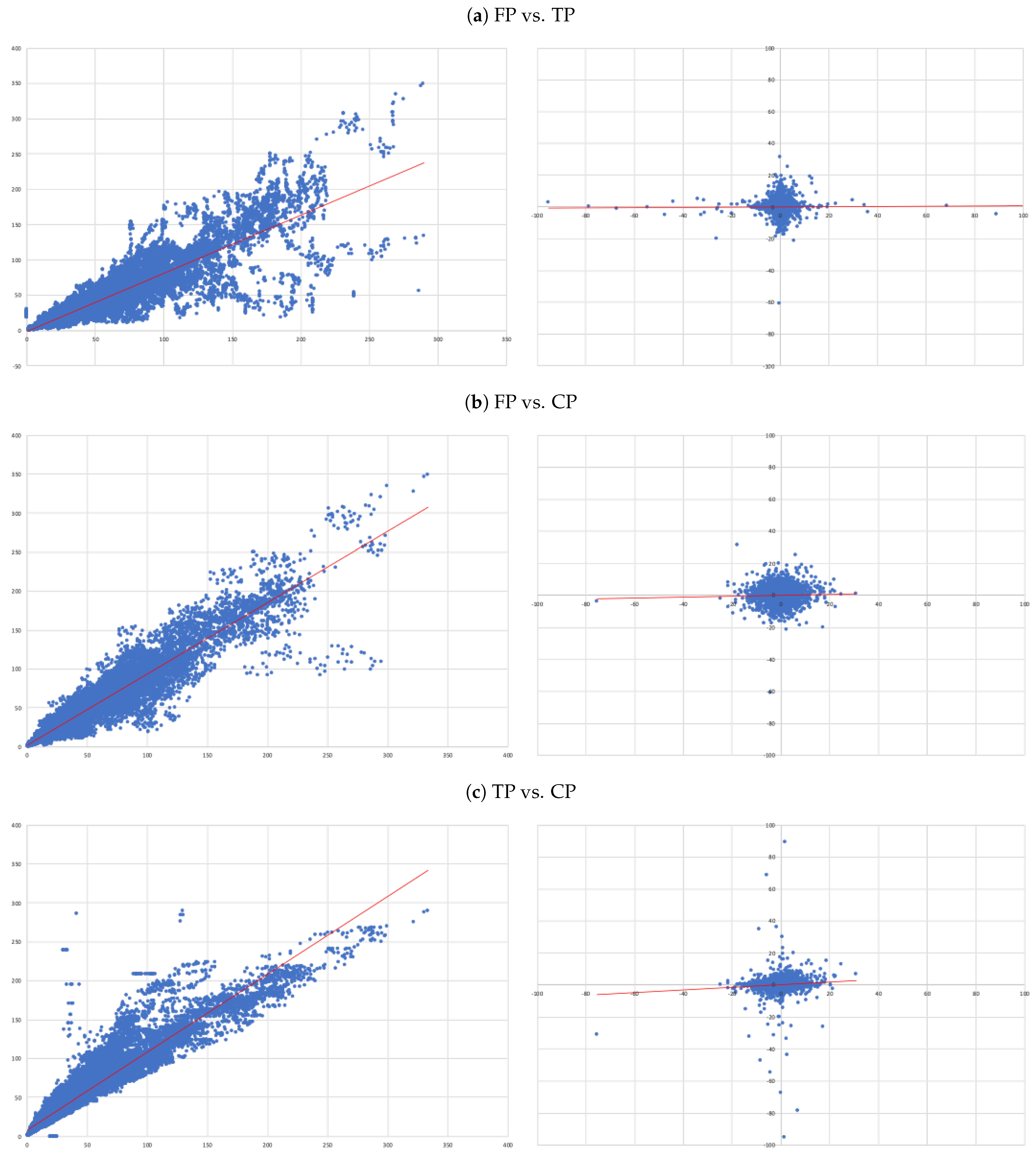
Thus, we look into three types of pairwise relationships:
- (A)
- FP vs. TP: we evaluate the accuracy of TP forecasts made by analysts.
- (B)
- FP vs. CP: to compare the accuracy of a forecast as naive as CP to analysts’ TP forecast.
- (C)
- TP vs. CP: to evaluate to what extent TP can be determined by CP.
The basic linear panel models used in econometrics can be described through suitable restrictions of the following general model:
where a represents a random disturbance term of mean 0.
In our case, is either (in (A) and (B) listed above) or (for (C)) and is either (in (A)) or (in (B) and (C)), with , and as in the variables Definition 1, whenever we are considering in level panel regressions. For in difference panel regressions, we consider its differences , , and accordingly.
Table 2 shows that our panel variables—FP, TP and CP—are non-stationary, but are integrated in the order of one1.
Therefore, when regressing our level panel variables on one another, one needs to be very careful with interpretations, as mostly there is likely nothing but spurious relationships. For further discussion on spurious relationship identification, see, for instance Granger and Newbold (2001). Despite this, intercept coefficients of in level panel regressions can be interpreted as optimism/pessimism indicators (forecast bias), when we use target prices as predictors of future prices. Likewise, when capitalised prices are used to predict future prices, intercept levels can be interpreted in terms of how much past returns over or under estimate future returns.
On the other hand, accuracy can only be properly evaluated from in differences panel regressions. For completeness, in Section 4 (or in the Appendix A), we present regression results both on levels and differences.
3.2.1. Overall Panel Regressions
We start by considering parameter homogeneity, i.e., and for all .
The resulting model
is a standard linear model pooling all the data across i and t.
This is the most common panel model and by considering fixed parameters, we aim to evaluate the overall relationship between y and x. Then, we consider two less restrictive models: cross-fixed effects models and period fixed effect models.
3.2.2. Panel Robustness
We checked the robustness of the overall panel regression results in two ways: by considering individual company fixed effects and by performing subperiod panel regressions.
To model individual company heterogeneity, we assume that the error term in (3) has two separate components,
is firm-specific and does not change over time, and is a random disturbance term of mean 0.
As in our case, it is likely that if the individual component is correlated with the regressors, the ordinary least squares (OLS) estimator of would be inconsistent, so it is customary to treat the as a further set of n parameters to be estimated, as if in the general model for all t.
In panel data terminology, are called fixed effects (otherwise known as within or least squares dummy variables) model, estimated by OLS on transformed data, guaranteeing consistent estimates for .
To test the robustness of our panel results over time, instead of considering time-fixed effects, we opted to take a different perspective, estimating additional panel regressions (as in (3)), for three subperiods:
- The pre-crisis period, until the end of August 2008;
- The crisis period, from September 2008 until the end of 2012;
- The pots crisis period, from 2013 onwards.
These are well-established subperiods for European stock markets2. When compared to a more formal structural break analysis, as proposed for instance in Okui and Wang (2021), considering these concrete sub-periods has the advantage of interpretability and comparability vis a vis the already vast literature around the financial crisis.
3.2.3. Individual Regressions
Finally, we also consider individual regressions, which is the same as allowing both coefficients and to vary for each firm i,
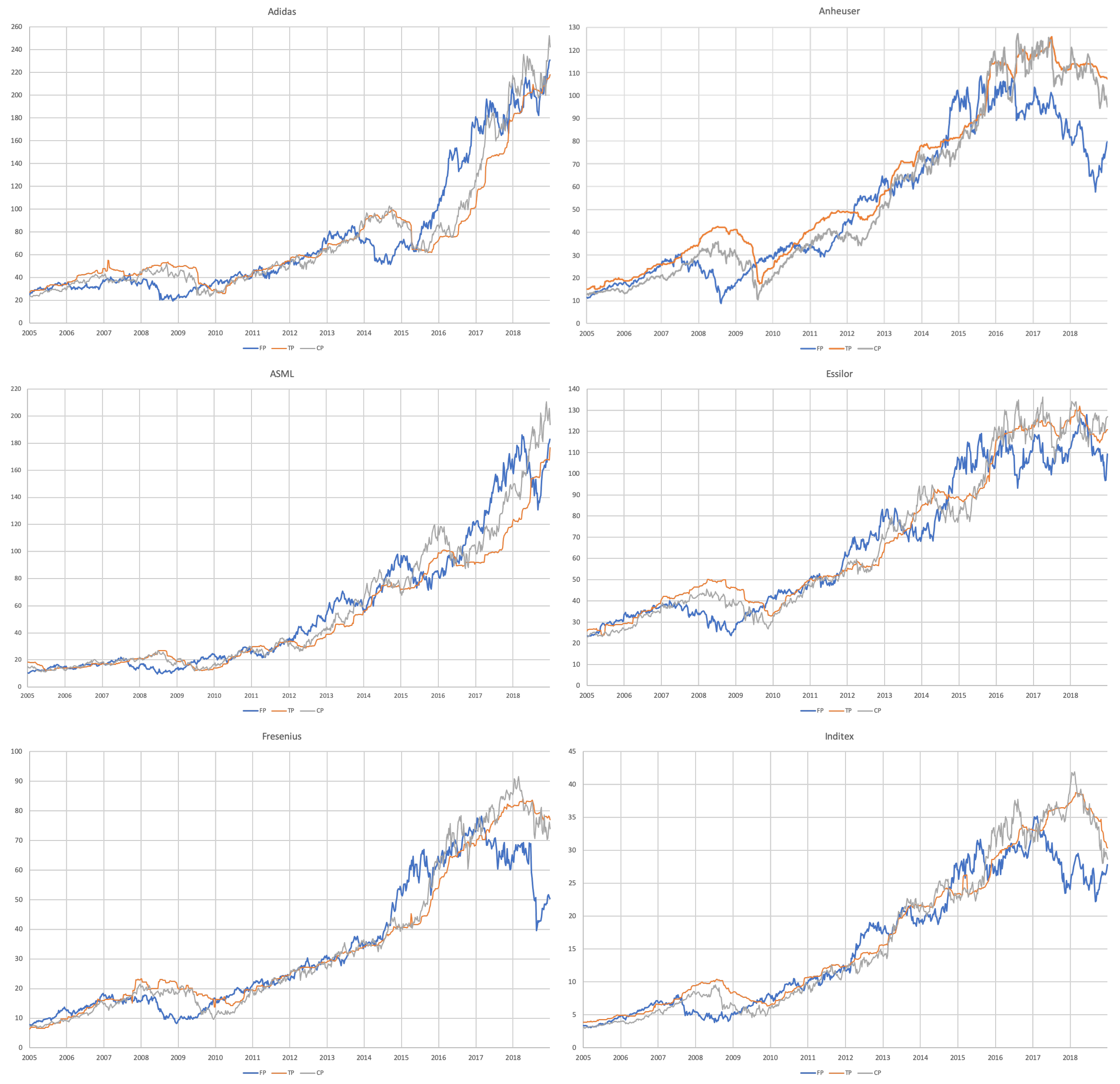
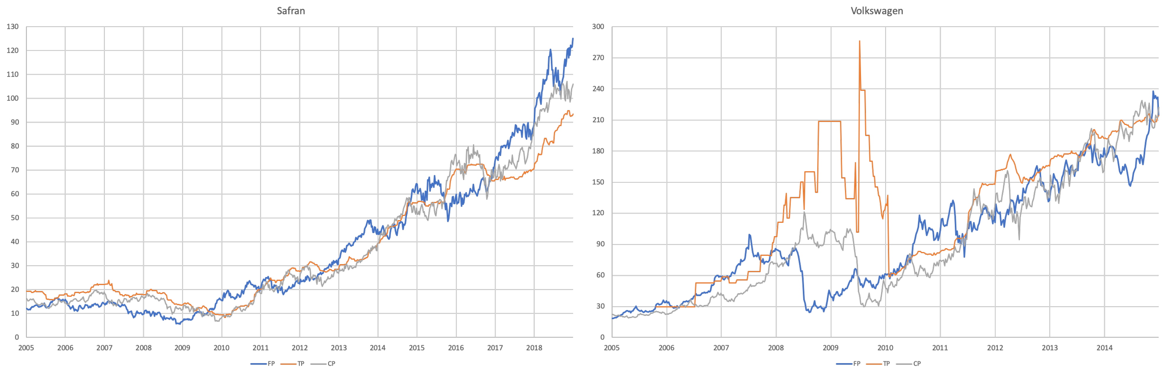
For illustration purposes, Figure 1 shows the evolution of the three variables—future prices (FP), target prices (TP) and capitalised prices (CP)—for the eight best performing companies over the 15-year period of our sample.
4. Results
4.1. Overall Panel Regressions
Table 3 summarises the overall panel regression results (Figure 2 illustrates them). As previously discussed, level regressions should be interpreted with extreme care, as we are dealing with non-stationary variables (recall results in Table 2). These relationships are indeed spurious as confirmed by the extremely small Durbin–Watson statistic values in Table 3 (0.019, 0.047 and 0.037)3. In practical terms, this means that, based upon level regressions, we cannot infer the relationship between the dependent and independent variables—we cannot interpret dependent variables coefficients nor use regression statistics to attest models quality. Still, we can interpret the constant coefficient and its significance.
From level results columns—(1), (3) and (5) in Table 3—we show evidence that:
- In our overall sample and on average, target prices overestimate future prices (positive and statistically significant negative );
- While capitalised prices tend to under estimate them (positive and statistically significant positive ).
This is in line with the literature attesting that the majority of target prices are too optimistic, supporting theoretical predictions by Ottaviani and Sørensen (2006), in line with the results of Bonini et al. (2010).
In terms of forecast accuracy, what can be interpreted are the results for the regressions in differences. From the analysis of the in difference results—columns (2), (4) and (6) in Table 3—we can conclude that:
- Overall, there is no evidence that target prices can forecast future prices—the second column of results in Table 3. In fact, the regression not only shows and of 0.000, but also the coefficient associated with the independent variable is also not statistically different from zero (as attested by its t-statistics);
- The ability capitalised prices have to explain analysts’ forecasts is very limited—sixth column of results in Table 3. In fact, we only get an . Nonetheless, in relative terms this regression is the “best”, as attested by the all model selection statistics.
4.2. Panel Robustness
Considering company fixed effects does not considerably change the “picture” in terms of accuracy (see in difference columns (2), (4) and (6) of Table A1, in the Appendix A), it seems that:
- The reason why, overall, our forecast variables (both TP and CP ) have no predicting power over future prices cannot be explained by firm-specific components.
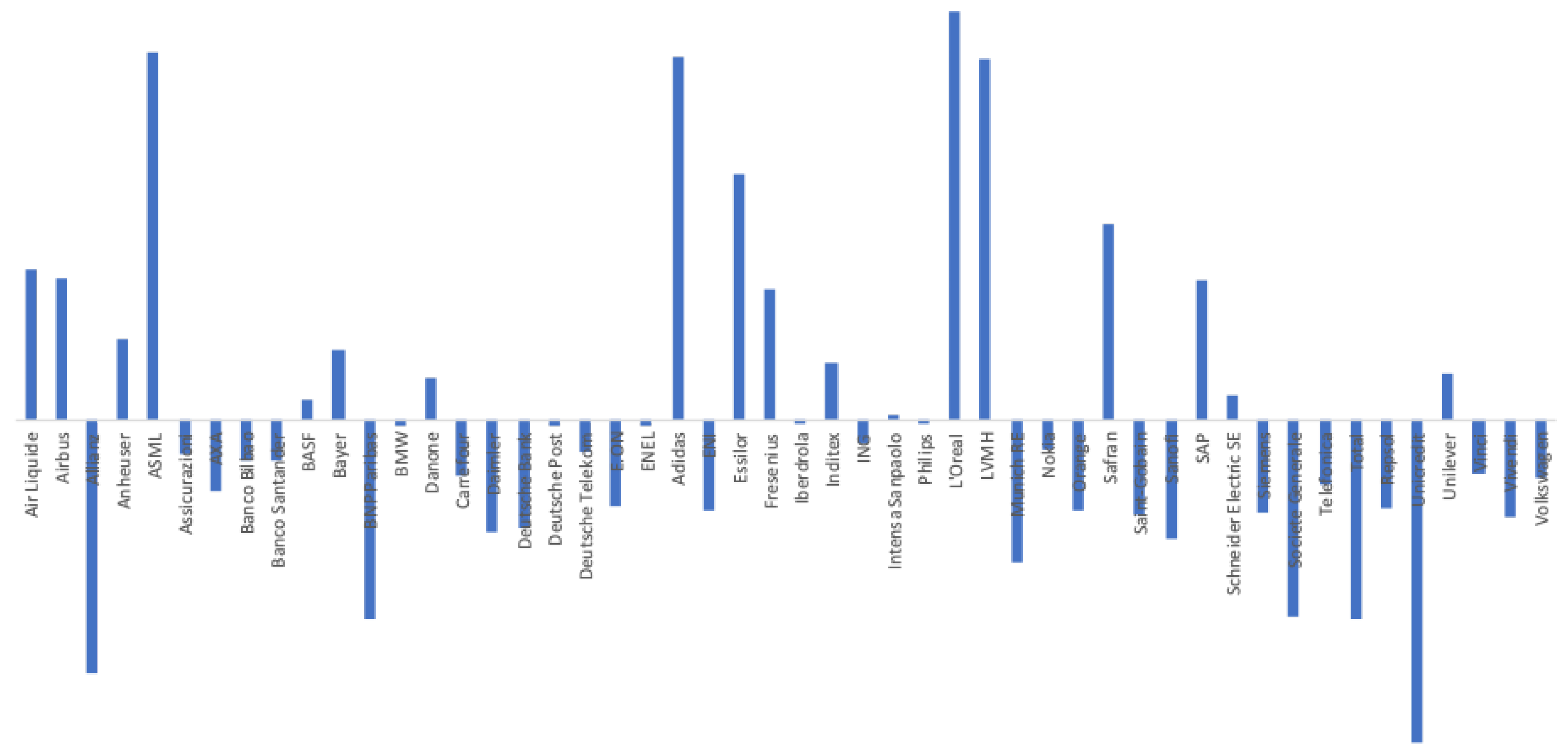
As before in the level regressions (columns (2), (4) and (6) of Table A1, in the Appendix A) are spurious. However, looking deeper into the variation of firm-specific estimates ( in Equation (4), illustrated at Figure 3), it seems we can conclude:
- Firm-specific variables may explain optimism/pessimism in target prices forecasts, as we obtained a wide range of values.
Results also do no change much, when considering panel regressions over the three proposed subperiods: pre-crisis, crisis and post-crisiss. Table 4 summarises the relevant statistics on the subperiod panel regressions (see full results for each of the subperiods in Table A2, Table A3 and Table A4, in the Appendix A).
Looking across periods its seems:
- Analysts became particularly pessimistic during the crisis-period (positive and significant crisis period level intercept) and optimistic in the post-crisis period (negative and significant for the equivalent post-crisis intercept);
- Absence of accuracy, of both target prices and capitalised prices, became even more severe during the crisis period (lowest adjusted ).
4.3. Individual Regressions
Perhaps most interesting are the individual sample results. Table 5, Table 6 and Table 7 show individual time series regressions for the eight best performing companies (the ones in Figure 1).
In general, when considering individual time series, the for in difference regressions increase.
- For each of the eight companies presented, the accuracy is not as bad as in the overall sample; the levels of the “FP vs TP” regressions range from 0.0012 (Inditex) to 0.1157 (Safran), suggesting that the accuracy of target prices is less than 12%, and varies considerably from firm to firm.
- Similarly, levels of the “FP vs CP” regressions range from 0.0021 (Essilor) to 0.1214 (Volkswagen), suggesting similar levels of accuracy of the two forecasts with target prices working better for some firms and capitalised prices for others.
- It is interesting that the highest levels are found for the “TP vs CP” regressions, where the levels range from 0.0904 (Fresenius) to as high as 0.3685 (Adidas), suggesting that at least between 10% and 35% of target prices can be explained by simple capitalisation rules.
5. Conclusions
Our empirical evidence indicates that, in the European stock market, Bloomberg’s consensus 12-month target prices are not accurate forecasts for future markets prices. It also shows that target prices by analysts do not even “beat” the accuracy of capitalised prices as forecasters of future prices (both do similarly bad).
This is at least the case for large capitalisation stocks, as our sample considers only stocks of the 50 European companies that stayed the longest in the Eurostoxx index between 2004 and 2019. If, as Falkenstein (1996) suggests, research intensity is positively related with accuracy, due to a learning effect, and, analogously, prediction errors are inversely related with some market factors such as size and liquidity, then accuracy for smaller cap companies is expected to be even worse.
Despite the spurious nature of in level panel regressions and the extreme low explanatory power of in difference regressions, we found evidence that the overall target prices are positively biased, as suggested by Ottaviani and Sørensen (2006), although, based upon our subperiod analysis, that was during the European crisis period (both global financial and sovereign debt), between September 2009 and 2012. In fact, during those times analysts were overall pessimistic.
The individual regression analysis seems to indicate the overall low accuracy may result from considerable variety in individual firm accuracy and size bias. Nonetheless, we still observed that target prices and capitalised prices are just slightly more accurate predictors of future prices and, if anything, capitalised prices seems to do better.
Although possibly polemical, from the industry perspective, our findings are in line with most of the academic literature.
One of the limitations of our analysis is the fact that we rely on Bloomberg consensus 12-month market prices that are averages of individual analysts’ forecasts. As suggested by Palley et al. (2019) and Tiberius and Lisiecki (2019), dispersion across analysts may also play a role. It could also be that a concrete analyst would perform much better (whilst others would need to perform worse) at particular time periods and/or for a particular set of companies. The debate on the performance (and survival) of “star” analysts goes on in the literature (see e.g., Bjerring et al. 1983; Desai et al. 2000).
However, unless the “good” forecasters are always the same , it is unlikely investors would risk following a particular analyst or set of analysts, instead of the industry consensus.
Author Contributions
Conceptualisation, R.M.G.; methodology, J.A. and R.M.G.; software, J.A.; validation, R.M.G.; formal analysis, R.M.G.; investigation, J.A. and R.M.G.; resources, J.A.; data curation, J.A.; writing—original draft preparation, R.M.G.; writing—review and editing, R.M.G.; visualisation, R.M.G.; supervision, R.M.G.; project administration, R.M.G.; funding acquisition, R.M.G. All authors have read and agreed to the published version of the manuscript.
Funding
R.M.G. was partially supported by the Project CEMAPRE/REM—UIDB/05069/2020 financed by FCT/MCTES (Portuguese Science Foundation), through national funds.
Data Availability Statement
This study uses data from Bloomberg.
Conflicts of Interest
The authors declare no conflict of interest.
Appendix A

Table A1.
Overall panel regression: cross-fixed effects.
| FP vs. TP | FP vs. CP | TP vs. CP | ||||
|---|---|---|---|---|---|---|
| (1) | (2) | (3) | (4) | (5) | (6) | |
| Dependent Variable | ||||||
| Mean dependent var | 38.516 | 0.070 | 38.516 | 0.070 | 48.456 | 0.057 |
| S.D. Dependent var | 39.241 | 1.839 | 39.241 | 1.839 | 42.886 | 1.758 |
| Intercept | ||||||
| Coefficient | −0. 811 | 0.069406 | 4.186 | 0.068 | 14.029 | 0.051 |
| Std. Error | 0.179 | 0.010 | 0.108 | 0.010 | 0.090 | 0.009 |
| t-Statistic | −4.532 | 7.212 | 38.883 | 7.033 | 153.288 | 5.542 |
| Prob. | 0.000 | 0. 0000 | 0.000 | 0.000 | 0.000 | 0.000 |
| Independent Variable | ||||||
| Coefficient | 0.812 | 0.004 | 0.857 | 0.026 | 0.859 | 0.080 |
| Std. Error | 0.003 | 0.005 | 0.002 | 0.005 | 0.002 | 0.005 |
| t-Statistic | 246.739 | 0.757 | 382.297 | 5.401 | 450.965 | 1.706 |
| Prob. | 0.000 | 0.449 | 0.000 | 0.000 | 0.000 | 0.000 |
| Regression Statistics | ||||||
| R-squared | 0.843 | 0.003 | 0.916 | 0.004 | 0.949 | 0.010 |
| Adjusted R-squared | 0.843 | 0.001 | 0.916 | 0.002 | 0.949 | 0.009 |
| S.E. Of regression | 15.544 | 1.838 | 11.350 | 1.837 | 9.649 | 1.750 |
| Sum square resid | 8,819,023 | 123,084 | 4,701,829 | 122,988 | 3,398,162 | 111,608 |
| Log Likelihood | −152,118 | −73,975 | −140,624 | −73,960 | −134,690 | −72,188 |
| F-statistic | 3928.6 | 2.014 | 8007.9 | 2.588 | 13,710 | 7.608 |
| Prob (F-statistic) | 0.000 | 0.000 | 0.000 | 0.000 | 0.000 | 0.000 |
| Model Statistics | ||||||
| AIC | 8.327 | 4.056 | 7.698 | 4.055 | 7.373 | 3.958 |
| BIC | 8.339 | 4.068 | 7.710 | 4.067 | 7.385 | 3.970 |
| HQC | 8.330 | 4.060 | 7.701 | 4.059 | 7.377 | 3.962 |
| Residuals Autocorr. | ||||||
| Durbi–Watson stat | 0.022 | 2.061 | 0.047 | 2.061 | 0.058 | 2.081 |
Regression results using panel least squares based upon 36550 balanced panel observations (with a total of 731 periods included and 50 cross-sections) with fixed effects. Panel variables are future prices (FP), target prices (TP) and capitalised prices (CP). Each column represents a specific panel regression as in Equations (4) and (5). We regress FP on TP, FP on CP and TP on CP, both in levels and differences. We report the model selection criteria of Akaike (1973) (AIC), (Schwarz et al. 1978) (SIC) and Hannan and Quinn (1979) (HQC). For residual autocorrelation, we used the panel data generalisation by Bhargava et al. (1982) of the classical Durbin and Watson (1950) statistic.
Table A2.
Pre-crisis period panel regressions.
| FP vs. TP | FP vs. CP | TP vs. CP | ||||
|---|---|---|---|---|---|---|
| (1) | (2) | (3) | (4) | (5) | (6) | |
| Dependent Variable | ||||||
| Mean dependent var | 28.077 | 0.035 | 28.077 | 0.035 | 41.649 | 0.135 |
| S.D. Dependent var | 23.214 | 1.196 | 23.214 | 1.196 | 35.118 | 1.750 |
| Intercept | ||||||
| Coefficient | 3.157 | 0.037 | 2.220 | 0.027 | 0.992 | 0.124 |
| Std. Error | 0.164 | 0.013 | 0.143 | 0.013 | 0.152 | 0.019 |
| t-Statistic | 19.289 | 2.873 | 15.503 | 2.135 | 6.527 | 6.590 |
| Prob. | 0.000 | 0.004 | 0.000 | 0.033 | 0.000 | 0.000 |
| Independent Variable | ||||||
| Coefficient | 0.598 | 0.017 | 0.931 | 0.089 | 1.464 | 0.132 |
| Std. Error | 0.003 | 0.007 | 0.004 | 0.013 | 0.004 | 0.020 |
| t-Statistic | 199.172 | −2.285 | 235.154 | 6.678 | 348.352 | 6.775 |
| Prob. | 0.000 | 0.022 | 0.000 | 0.000 | 0.000 | 0.000 |
| Regression Statistics | ||||||
| R-squared | 0.819 | 0.001 | 0.863 | 0.005 | 0.933 | 0.005 |
| Adjusted R-squared | 0.819 | 0.000 | 0.863 | 0.005 | 0.933 | 0.005 |
| S.E. of regression | 9.868 | 1.195 | 8.580 | 1.193 | 9.107 | 1.746 |
| Sum square resid | 851,841 | 12,426 | 643,983 | 12,370 | 725,530 | 26,514 |
| Log Likelihood | −32,446 | −13,895 | −31,222 | −13,876 | −31,744 | −17,192 |
| F-statistic | 39,670 | 5.220 | 55,297 | 4.460 | 121,349 | 45.898 |
| Prob (F-statistic) | 0.000 | 0.022 | 0.000 | 0.000 | 0.000 | 0.000 |
| Model Statistics | ||||||
| AAIC | 7.417 | 3.195 | 7.137 | 3.190 | 7.256 | 3.953 |
| SIC | 7.418 | 3.196 | 7.139 | 3.192 | 7.258 | 3.954 |
| HQC | 7.417 | 3.195 | 7.138 | 3.191 | 7.257 | 3.953 |
| Residuals Autocorr. | ||||||
| Durbi–Watson stat | 0.027 | 2.072 | 0.028 | 2.067 | 0.056 | 1.944 |
Regression results using panel least squares based upon 8750 balanced panel observations (with a total of 135 periods included and 50 cross-sections). Panel variables are future prices (FP), target prices (TP) and capitalised prices (CP). Each column represents a specific panel regression as in Equation (3). We regress FP on TP, FP on CP and TP on CP, both in levels and differences. We report the model selection criteria of Akaike (1973) (AIC), (Schwarz et al. 1978) (SIC) and Hannan and Quinn (1979) (HQC). For residual autocorrelation, we used the panel data generalisation by Bhargava et al. (1982) of the classical Durbin and Watson (1950) statistic.
Table A3.
Crisis period panel regressions.
| FP vs. TP | FP vs. CP | TP vs. CP | ||||
|---|---|---|---|---|---|---|
| (1) | (2) | (3) | (4) | (5) | (6) | |
| Dependent Variable | ||||||
| Mean dependent var | 26.324 | 0.038 | 26.324 | 0.038 | 41.647 | 0.073 |
| S.D. Dependent var | 22.156 | 1.582 | 22.156 | 1.582 | 33.856 | 2.539 |
| Intercept | ||||||
| Coefficient | 5.468 | 0.038 | 2.480 | 0.038 | 3.087 | 0.072 |
| Std. Error | 0.213 | 0.015 | 0.158 | 0.015 | 0.187 | 0.024 |
| t-Statistic | 25.705 | 2.557 | 15.672 | 2 557854 | 16.495 | −3.008 |
| Prob. | 0.000 | 0.011 | 0.000 | 0.011 | 0.000 | 0.003 |
| Independent Variable | ||||||
| Coefficient | 0.501 | 0.000 | 0.816 | 0.001 | 1.320 | 0.026 |
| Std. Error | 0.004 | 0.006 | 0.004 | 0.008 | 0.005 | 0.013 |
| t-Statistic | 126.367 | 0.057 | 194.373 | 0.117 | 265.826 | 1.947 |
| Prob. | 0.000 | 0.954 | 0.000 | 0.907 | 0.000 | 0.052 |
| Regression Statistics | ||||||
| R-squared | 0.586 | 0.000 | 0.770 | 0.000 | 0.862 | 0.000 |
| Adjusted R-squared | 0.586 | 0.000 | 0.770 | 0.000 | 0.862 | 0.000 |
| S.E. of regression | 14.262 | 1.582 | 10.631 | 1.582 | 12.570 | 2.539 |
| Sum square resid | 2,298,141 | 28,138 | 1,276,771 | 28,138 | 1,785,249 | 72,490 |
| Log Likelihood | −46,064 | −21,120 | −42,743 | −21,120 | −44,637 | −26,443 |
| F-statistic | 15,969 | 0.003 | 37,781 | 0.014 | 70,664 | 3.791 |
| Prob (F-statistic) | 0.000 | 0.954 | 0.000 | 0.907 | 0.000 | 0.052 |
| Model Statistics | ||||||
| AIC | 8.153 | 3.755 | 7.566 | 3.755 | 7.901 | 4.701 |
| SIC | 8.155 | 3.756 | 7.567 | 3.756 | 7.902 | 4.703 |
| HQC | 8.154 | 3.755 | 7.566 | 3.755 | 7.901 | 4.702 |
| Residuals Autocorr. | ||||||
| Durbi–Watson stat | 0.0203 | 2.2066 | 0.0417 | 2.2067 | 0.0761 | 2.2790 |
Regression results using panel least squares based upon 11300 balanced panel observations (with a total of 226 periods included and 50 cross-sections). Panel variables are future prices (FP), target prices (TP) and capitalised prices (CP). Each column represents a specific panel regression as in Equation (3). We regress FP on TP, FP on CP and TP on CP, both in levels and differences. We report the model selection criteria of Akaike (1973) (AIC), (Schwarz et al. 1978) (SIC) and Hannan and Quinn (1979) (HQC). For residual autocorrelation, we used the panel data generalisation by Bhargava et al. (1982) of the classical Durbin and Watson (1950) statistic.
Table A4.
Post-crisis period panel regressions.
| FP vs. TP | FP vs. CP | TP vs. CP | ||||
|---|---|---|---|---|---|---|
| (1) | (2) | (3) | (4) | (5) | (6) | |
| Dependent Variable | ||||||
| Mean dependent var | 52.401 | 0.107 | 52.401 | 0.107 | 56.730 | 0.106 |
| S.D. Dependent var | 49.365 | 2.242 | 49.365 | 2.242 | 50.105 | 0.895 |
| Intercept | ||||||
| Coefficient | −1.026 | 0.098 | 2.701 | 0.103 | 5.021 | 0.093 |
| Std. Error | 0.170 | 0.018 | 0.150 | 0.017 | 0.090 | 0.007 |
| t-Statistic | −6.016 | 5.562 | 18.063 | 5.862 | 55.952 | 13.744 |
| Prob. | 0.000 | 0.000 | 0.000 | 0.000 | 0.000 | 0.000 |
| Independent Variable | ||||||
| Coefficient | 0.942 | 0.086 | 0.919 | 0.033 | 0.957 | 0.097 |
| Std. Error | 0.002 | 0.020 | 0.002 | 0.007 | 0.001 | 0.003 |
| t-Statisti | 418.079 | 4.406 | 459.943 | 4.518 | 797.498 | 34.875 |
| Prob. | 0.000 | 0.000 | 0.000 | 0.000 | 0.000 | 0.000 |
| Regression Statistics | ||||||
| R-squared | 0.914 | 0.001 | 0.928 | 0.001 | 0.975 | 0.069 |
| Adjusted R-squared | 0.914 | 0.001 | 0.928 | 0.001 | 0.975 | 0.069 |
| S.E. of regression | 14.498 | 2.241 | 13.278 | 2.241 | 7.967 | 0.864 |
| Sum square resid | 3,467,636 | 82,572 | 2,908,700 | 82,567 | 1,047,283 | 12,266 |
| Log Likelihood | −67,532 | −36,611 | −66,082 | −36,611 | −57,655 | −20,927 |
| F-statistic | 174,790 | 1.941 | 211,548 | 2.041 | 636,003 | 1216 |
| Prob (F-statistic) | 0.000 | 0.000 | 0.000 | 0.000 | 0.000 | 0.000 |
| Model Statistics | ||||||
| AIC | 8.186 | 4.451 | 8.010 | 4.451 | 6.989 | 2.545 |
| SIC | 8.187 | 4.452 | 8.011 | 4.452 | 6.990 | 2.546 |
| HQC | 8.186 | 4.452 | 8.011 | 4.452 | 6.989 | 2.545 |
| Residuals Autocorr. | ||||||
| Durbi–Watson stat | 0.027 | 2.009 | 0.054 | 2.005 | 0.079 | 1.306 |
Regression results using panel least squares based upon 16500 balanced panel observations (with a total of 330 periods included and 50 cross-sections). Panel variables are future prices (FP), target prices (TP) and capitalised prices (CP). Each column represents a specific panel regression as in Equation (3). We regress FP on TP, FP on CP and TP on CP, both in levels and differences. We report the model selection criteria of Akaike (1973) (AIC), (Schwarz et al. 1978) (SIC) and Hannan and Quinn (1979) (HQC). For residual autocorrelation, we used the panel data generalisation by Bhargava et al. (1982) of the classical Durbin and Watson (1950) statistic.
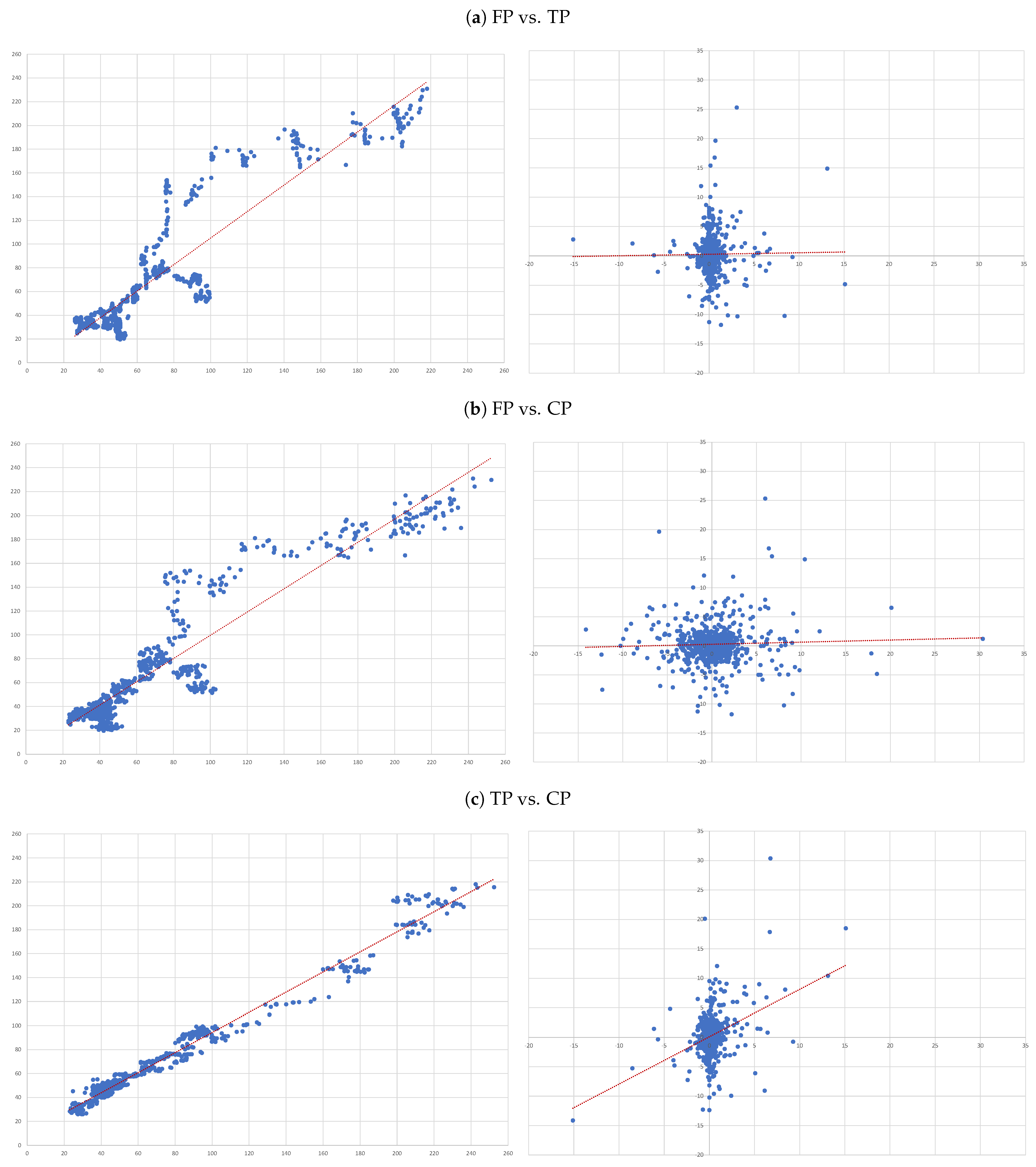
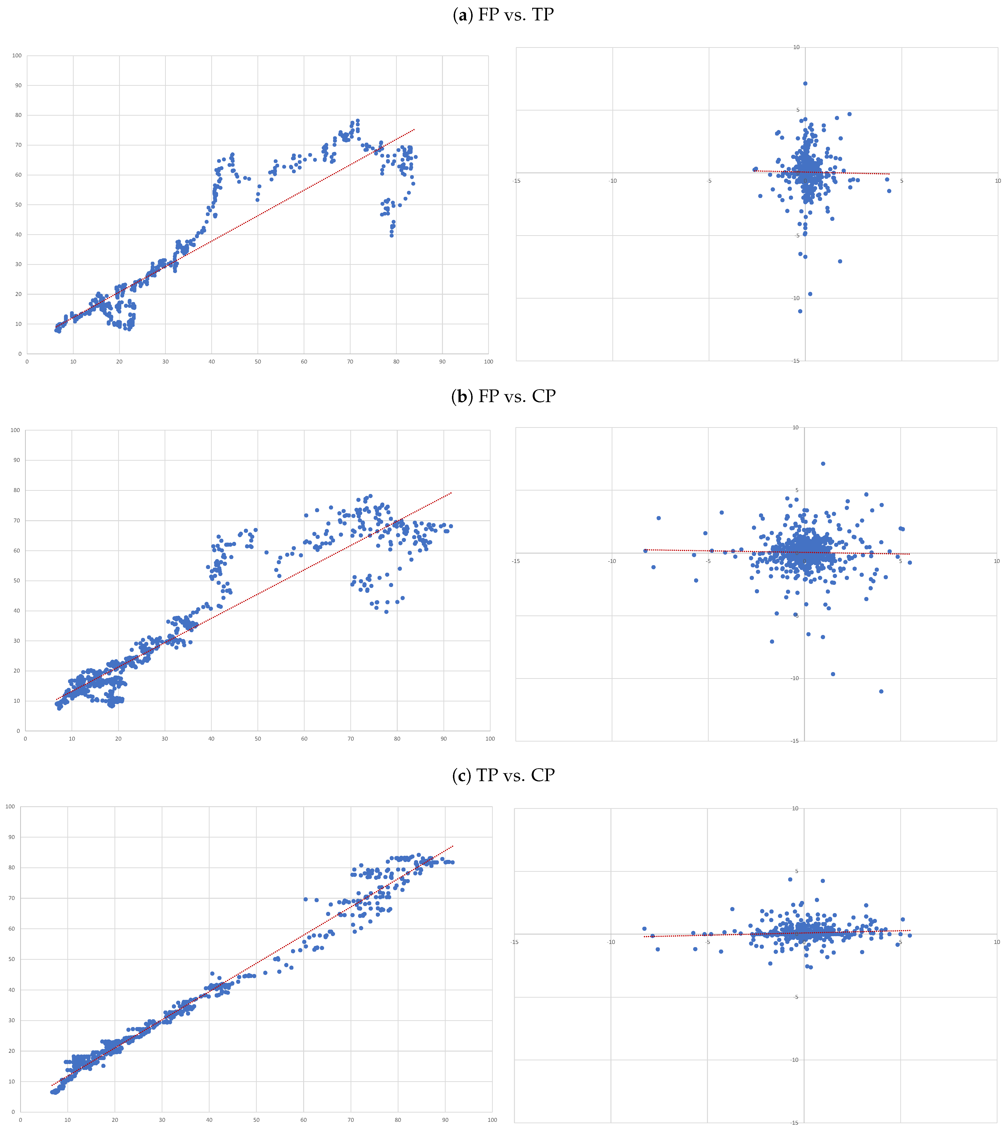
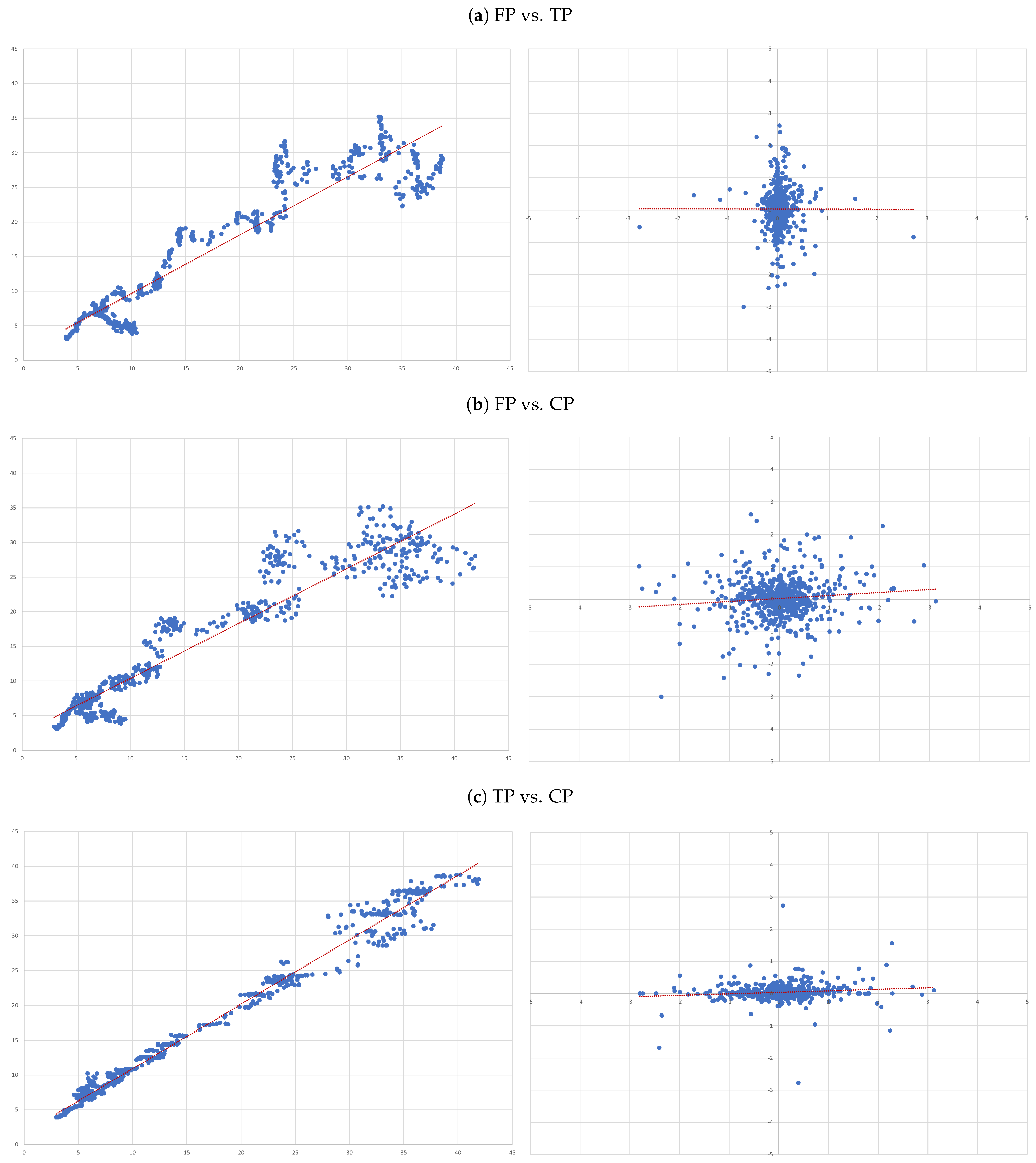
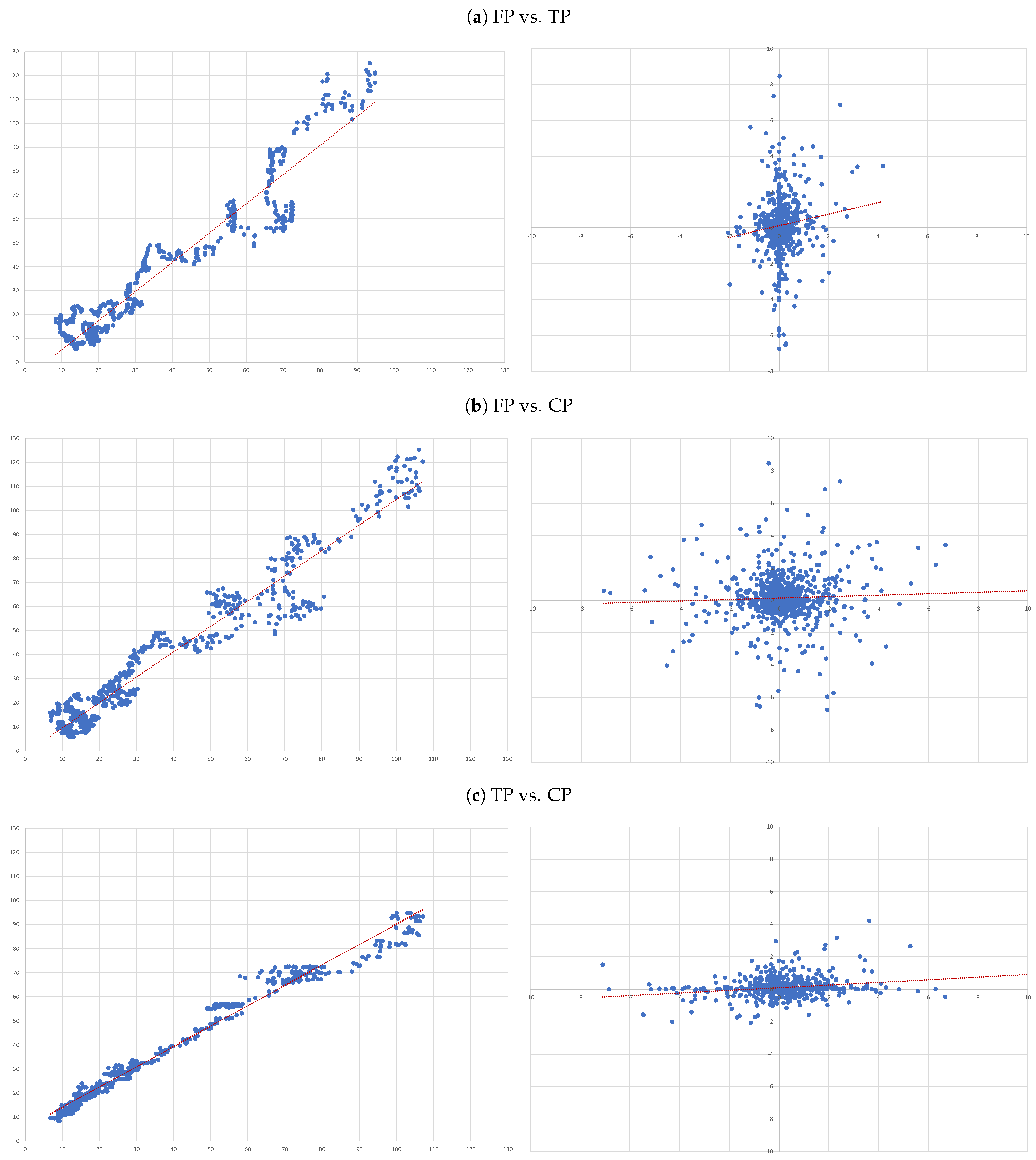
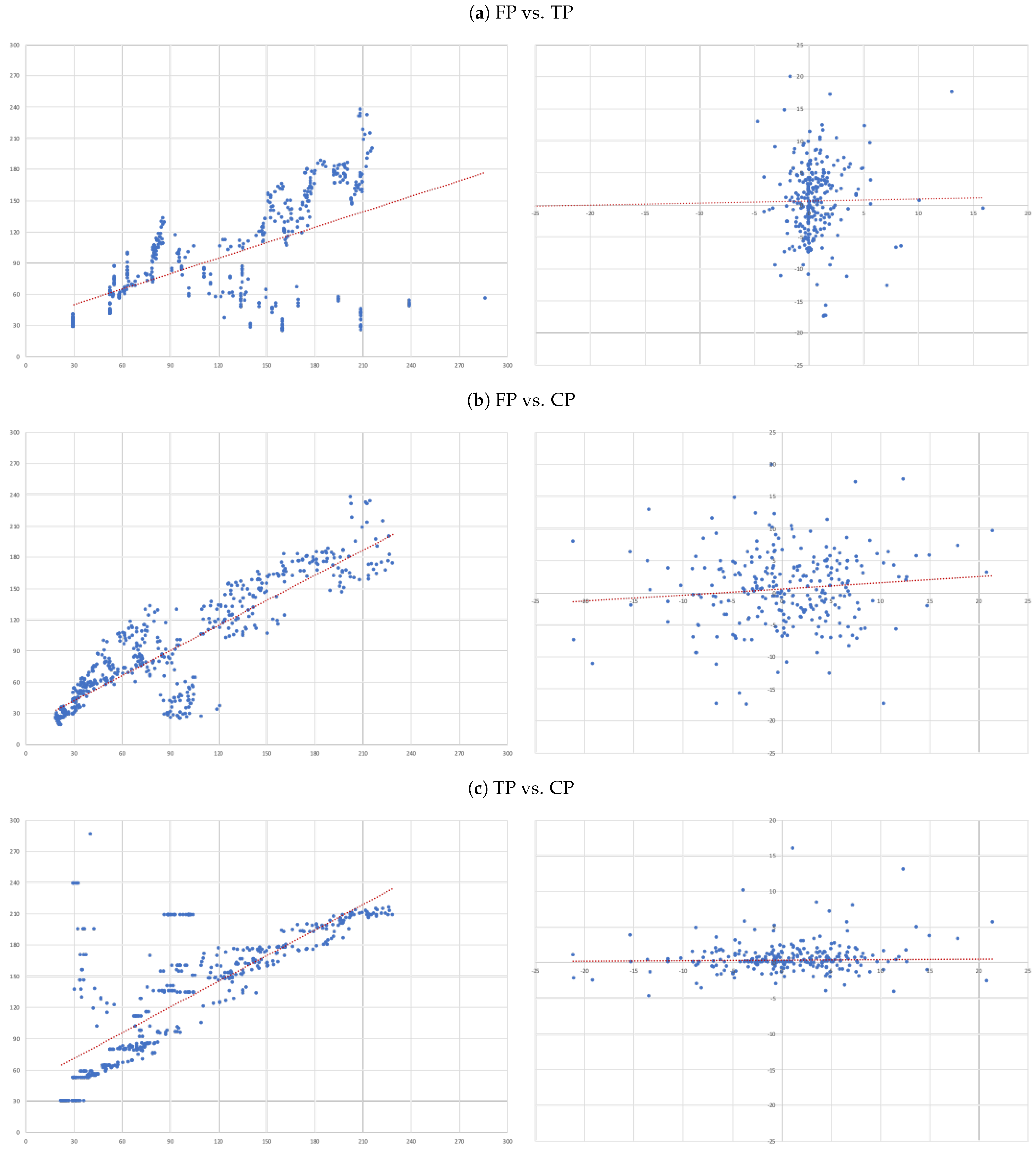
Figure A1.
Adidas. Individual time series regressions using three price series on Adidas: future prices (FP), target prices (TP), and capitalised prices (CP) forecasts. On the left-hand-side are images of level regressions and on the right-hand-side are the regressions in differences.
Figure A1.
Adidas. Individual time series regressions using three price series on Adidas: future prices (FP), target prices (TP), and capitalised prices (CP) forecasts. On the left-hand-side are images of level regressions and on the right-hand-side are the regressions in differences.

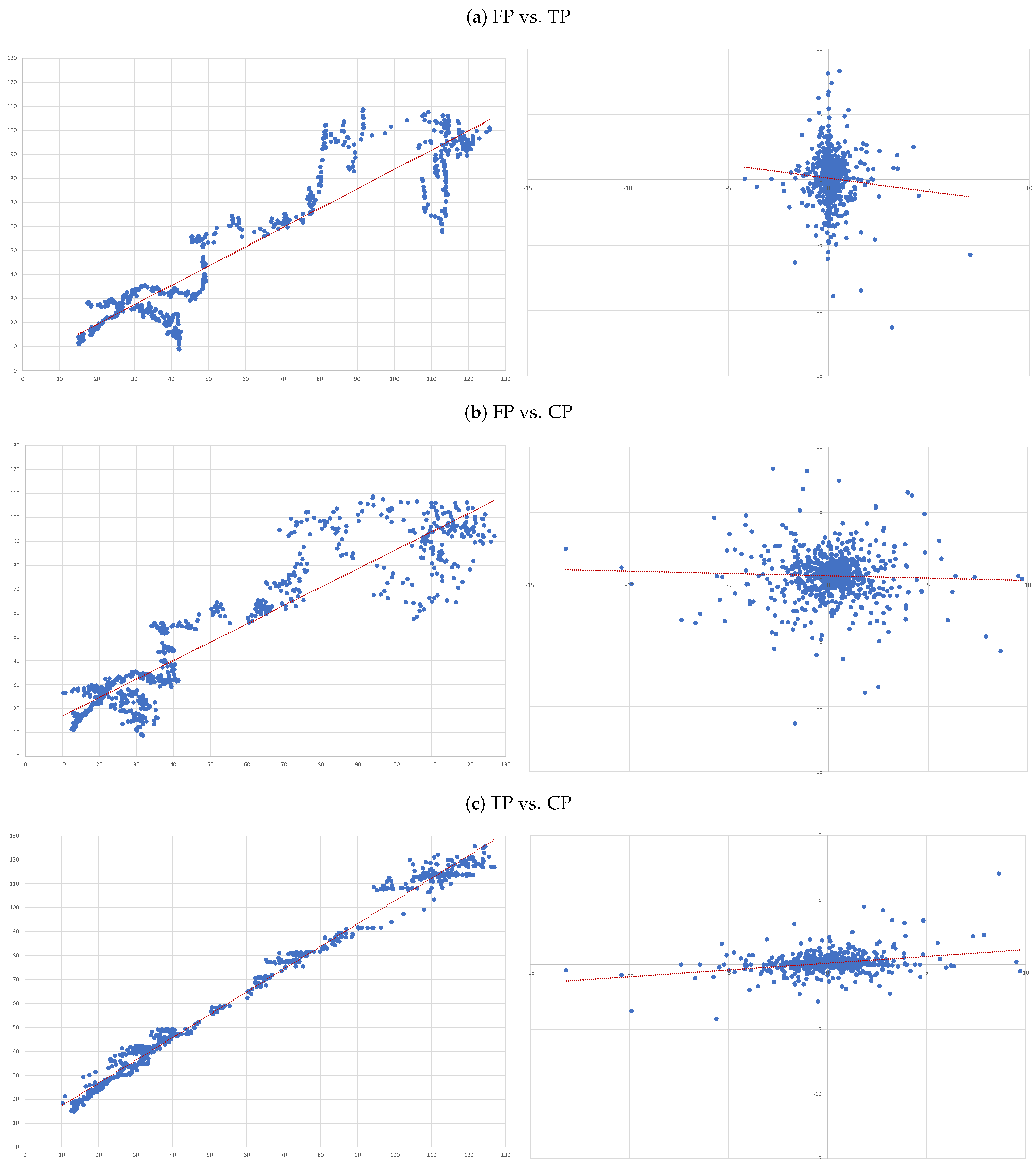
Figure A2.
Anheuser. Individual time series regressions using three price series on Anheuser: future prices (FP), target prices (TP), and capitalised prices (CP) forecasts. On the left-hand-side images of level regressions and on the right-hand-side of regressions in differences.
Figure A2.
Anheuser. Individual time series regressions using three price series on Anheuser: future prices (FP), target prices (TP), and capitalised prices (CP) forecasts. On the left-hand-side images of level regressions and on the right-hand-side of regressions in differences.

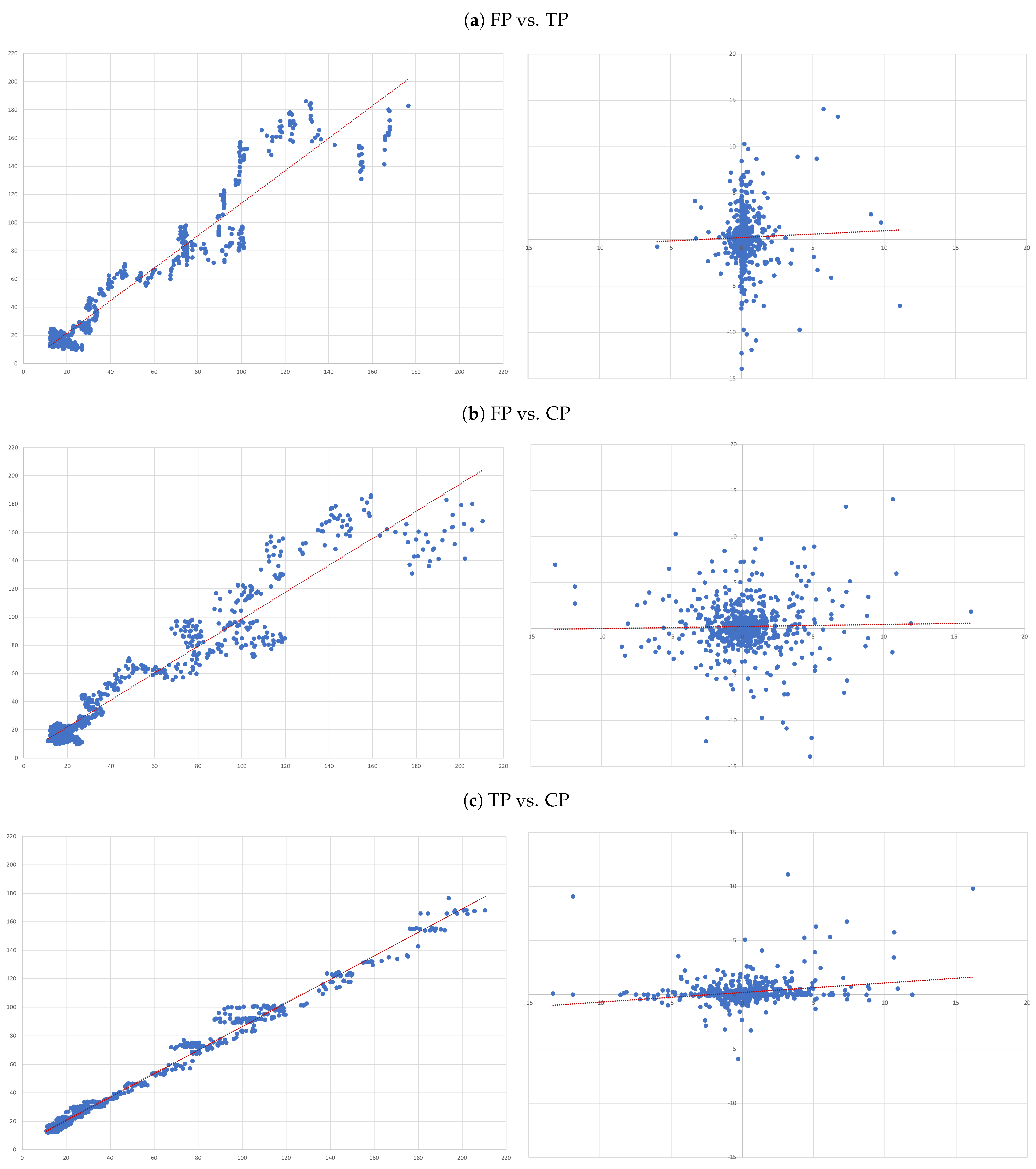
Figure A3.
ASML. Individual time series regressions using three price series on ASML: future prices (FP), target prices (TP), and capitalised prices (CP) forecasts. On the left-hand-side are images of level regressions and on the right-hand-side are regressions in differences.
Figure A3.
ASML. Individual time series regressions using three price series on ASML: future prices (FP), target prices (TP), and capitalised prices (CP) forecasts. On the left-hand-side are images of level regressions and on the right-hand-side are regressions in differences.

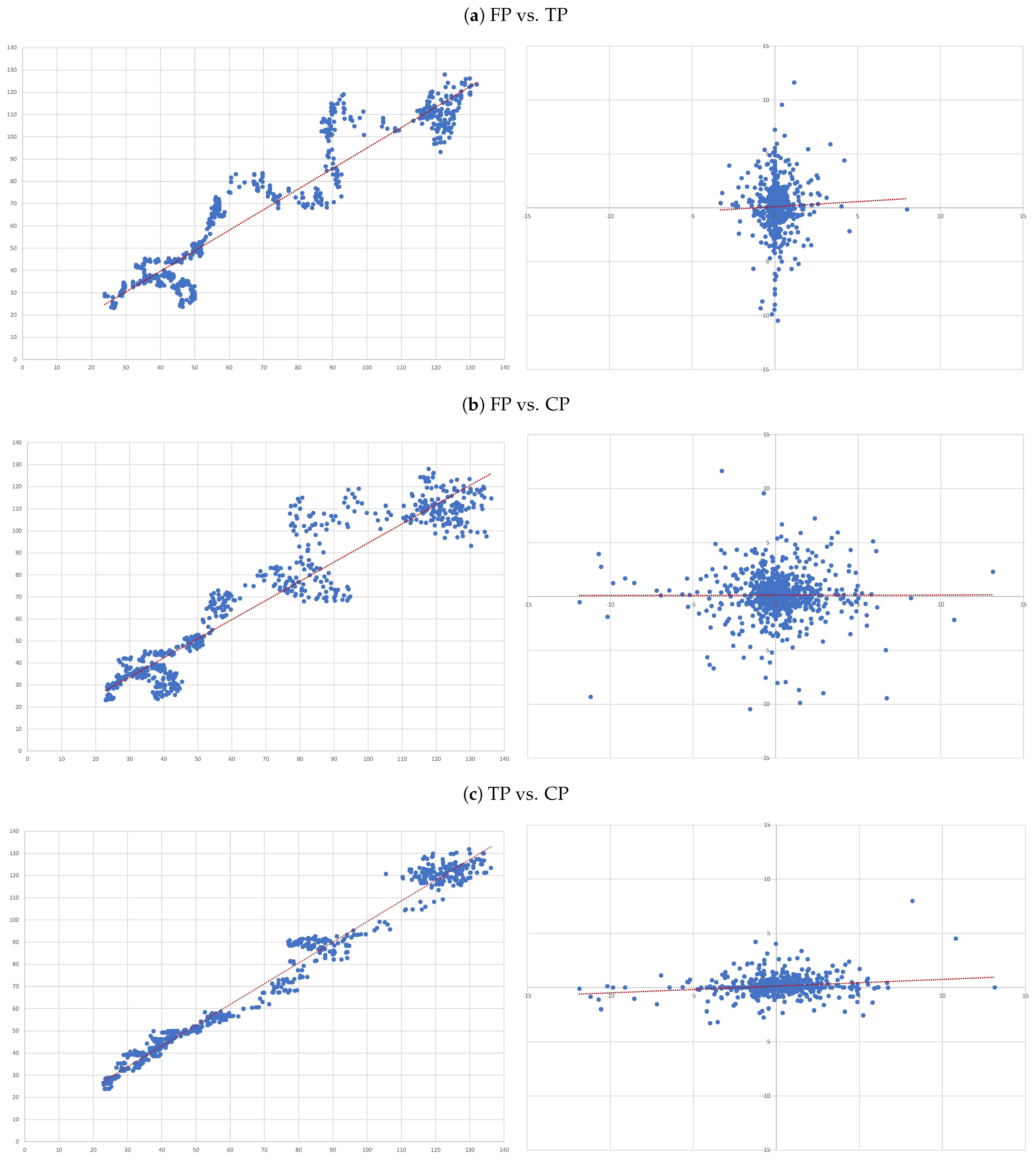
Figure A4.
Essilor. Individual time series regressions using three price series on Essilor: future prices (FP), target prices (TP), and capitalised prices (CP) forecasts. On the left-hand-side are images of level regressions and on the right-hand-side are regressions in differences.
Figure A4.
Essilor. Individual time series regressions using three price series on Essilor: future prices (FP), target prices (TP), and capitalised prices (CP) forecasts. On the left-hand-side are images of level regressions and on the right-hand-side are regressions in differences.

Figure A5.
Fresenius. Individual time series regressions using three price series on Fresenius: future prices (FP), target prices (TP), and capitalised prices (CP) forecasts. On the left-hand-side are images of level regressions and on the right-hand-side are regressions in differences.
Figure A5.
Fresenius. Individual time series regressions using three price series on Fresenius: future prices (FP), target prices (TP), and capitalised prices (CP) forecasts. On the left-hand-side are images of level regressions and on the right-hand-side are regressions in differences.

Figure A6.
Inditex. Individual time series regressions using three price series on Inditex: future prices (FP), target prices (TP), and capitalised prices (CP) forecasts. On the left-hand-side are images of level regressions and on the right-hand-side are regressions in differences.
Figure A6.
Inditex. Individual time series regressions using three price series on Inditex: future prices (FP), target prices (TP), and capitalised prices (CP) forecasts. On the left-hand-side are images of level regressions and on the right-hand-side are regressions in differences.

Figure A7.
Safran. Individual time series regressions using three price series on Safran: future prices (FP), target prices (TP), and capitalised prices (CP) forecasts. On the left-hand-side are images of level regressions and on the right-hand-side are regressions in differences.
Figure A7.
Safran. Individual time series regressions using three price series on Safran: future prices (FP), target prices (TP), and capitalised prices (CP) forecasts. On the left-hand-side are images of level regressions and on the right-hand-side are regressions in differences.

Figure A8.
Volkswagen. Individual time series regressions using three price series on Volkswagen: future prices (FP), target prices (TP), and capitalised prices (CP) forecasts. On the left-hand-side are images of level regressions and on the right-hand-side are regressions in differences.
Figure A8.
Volkswagen. Individual time series regressions using three price series on Volkswagen: future prices (FP), target prices (TP), and capitalised prices (CP) forecasts. On the left-hand-side are images of level regressions and on the right-hand-side are regressions in differences.

| 1 | “Order of integration” is a summary statistic used to describe a unit root process in time series analysis. Specifically, it tells you the minimum number of differences needed to obtain a stationary series (Engle and Granger 1991). |
| 2 | Our crisis period includes both the global financial crisis and the European sovereign debt crisis. |
| 3 | According to Granger and Newbold (2001), we should suspect that a regression is spurious if , where d is the Durbin–Watson statistic, which is the case for all level regressions and not the case for the regressions in differences. |
References
- Abdel-Khalik, A. Rashad, and Bipin B. Ajinkya. 1982. Returns to informational advantages: The case of analysts’ forecast revisions. Accounting Review 57: 661–80. [Google Scholar]
- Admati, Anat R., and Paul Pfleiderer. 1997. Does it all add up? benchmarks and the compensation of active portfolio managers. The Journal of Business 70: 323–50. [Google Scholar] [CrossRef] [Green Version]
- Akaike, Hirotogu. 1973. Information theory as an extension of the maximum likelihood. In IEEE International Symposium on Information Theory. Budapest: Akadémiai Kiadó. [Google Scholar]
- Asquith, Paul, Michael B. Mikhail, and Andrea S. Au. 2005. Information content of equity analyst reports. Journal of Financial Economics 75: 245–82. [Google Scholar] [CrossRef] [Green Version]
- Barber, Brad, Reuven Lehavy, Maureen McNichols, and Brett Trueman. 2001. Can investors profit from the prophets? security analyst recommendations and stock returns. The Journal of Finance 56: 531–63. [Google Scholar] [CrossRef]
- Barr Rosenberg, Kenneth Reid, and Ronald Lanstein. 1984. Persuasive evidence of market inefficiency. Journal of Portfolio Management 11: 9–17. [Google Scholar] [CrossRef]
- Bhargava, Alok, Luisa Franzini, and Wiji Narendranathan. 1982. Serial correlation and the fixed effects model. The Review of Economic Studies 49: 533–49. [Google Scholar] [CrossRef]
- Bilinski, Pawel, Danielle Lyssimachou, and Martin Walker. 2013. Target price accuracy: International evidence. The Accounting Review 88: 825–51. [Google Scholar] [CrossRef]
- Bjerring, James H, Josef Lakonishok, and Theo Vermaelen. 1983. Stock prices and financial analysts’ recommendations. The Journal of Finance 38: 187–204. [Google Scholar] [CrossRef]
- Bonini, Stefano, Laura Zanetti, Roberto Bianchini, and Antonio Salvi. 2010. Target price accuracy in equity research. Journal of Business Finance & Accounting 37: 1177–217. [Google Scholar]
- Bradshaw, Mark, Alan Huang, and Hongping Tan. 2014. Analyst Target Price Optimism around the World. Working Paper. Chestnut Hill: Boston College. [Google Scholar]
- Bradshaw, Mark T., Lawrence D. Brown, and Kelly Huang. 2013. Do sell-side analysts exhibit differential target price forecasting ability? Review of Accounting Studies 18: 930–55. [Google Scholar] [CrossRef]
- Bradshaw, Mark T., Alan G. Huang, and Hongping Tan. 2019. The effects of analyst-country institutions on biased research: Evidence from target prices. Journal of Accounting Research 57: 85–120. [Google Scholar] [CrossRef] [Green Version]
- Bradshaw, Mark T., Lian Fen Lee, and Kyle Peterson. 2016. The interactive role of difficulty and incentives in explaining the annual earnings forecast walkdown. The Accounting Review 91: 995–1021. [Google Scholar] [CrossRef] [Green Version]
- Brav, Alon, and Reuven Lehavy. 2003. An empirical analysis of analysts’ target prices: Short-term informativeness and long-term dynamics. The Journal of Finance 58: 1933–67. [Google Scholar] [CrossRef]
- Calomiris, Charles W., and Joseph R. Mason. 1997. Contagion and bank failures during the great depression: The june 1932 chicago banking panic. The American Economic Review 87: 863–883. [Google Scholar]
- Cao, Charles, Bing Liang, Andrew W. Lo, and Lubomir Petrasek. 2017. Hedge fund holdings and stock market efficiency. The Review of Asset Pricing Studies 8: 77–116. [Google Scholar] [CrossRef]
- Cheng, Lee-Young, Yi-Chen Su, Zhipeng Yan, and Yan Zhao. 2019. Corporate governance and target price accuracy. International Review of Financial Analysis 64: 93–101. [Google Scholar] [CrossRef]
- Choi, In. 2001. Unit root tests for panel data. Journal of International Money and Finance 20: 249–72. [Google Scholar] [CrossRef]
- Da, Zhi, Keejae P. Hong, and Sangwoo Lee. 2016. What drives target price forecasts and their investment value? Journal of Business Finance & Accounting 43: 487–510. [Google Scholar]
- Da, Zhi, and Ernst Schaumburg. 2011. Relative valuation and analyst target price forecasts. Journal of Financial Markets 14: 161–92. [Google Scholar] [CrossRef]
- Desai, Hemang, Bing Liang, and Ajai K. Singh. 2000. Do all-stars shine? evaluation of analyst recommendations. Financial Analysts Journal 56: 20–29. [Google Scholar] [CrossRef]
- Dimson, Elroy, and Massoud Mussavian. 1998. A brief history of market efficiency. European Financial Management 4: 91–103. [Google Scholar] [CrossRef] [Green Version]
- Durbin, James, and Geoffrey S. Watson. 1950. Testing for serial correlation in least squares regression: I. Biometrika 37: 409–28. [Google Scholar] [PubMed]
- Elton, Edwin J., Martin J. Gruber, and Andre de Souza. 2019. Are passive funds really superior investments? an investor perspective. Financial Analysts Journal 73: 7–19. [Google Scholar] [CrossRef] [Green Version]
- Engelberg, Joseph, R. David McLean, and Jeffrey Pontiff. 2020. Analysts and anomalies. Journal of Accounting and Economics 69: 101249. [Google Scholar] [CrossRef]
- Engle, Robert, and Clive Granger. 1991. Long-Run Economic Relationships: Readings in Cointegration. Oxford: Oxford University Press. [Google Scholar]
- Falkenstein, Eric G. 1996. Preferences for stock characteristics as revealed by mutual fund portfolio holdings. The Journal of Finance 51: 111–35. [Google Scholar] [CrossRef]
- Fama, Eugene F. 1965. The behavior of stock-market prices. The Journal of Business 38: 34–105. [Google Scholar] [CrossRef]
- Fama, Eugene F., Lawrence Fisher, Michael C. Jensen, and Richard Roll. 1969. The adjustment of stock prices to new information. International Economic Review 10: 1–21. [Google Scholar] [CrossRef]
- Farmer, Roger E. A. 1999. Macroeconomics of Self-Fulfilling Prophecies. Cambridge: MIT Press. [Google Scholar]
- French, Kenneth R. 2008. Presidential address: The cost of active investing. The Journal of Finance 63: 1537–73. [Google Scholar] [CrossRef]
- Garber, Peter M. 1989. Tulipmania. Journal of Political Economy 97: 535–60. [Google Scholar] [CrossRef]
- Granger, Clive W. J., and Paul Newbold. 2001. Spurious regressions in econometrics. In Essays in Econometrics: Collected Papers of Clive WJ Granger vol.32. Cambridge: Cambridge University Press, pp. 109–18. [Google Scholar]
- Hannan, Edward J., and Barry G. Quinn. 1979. The determination of the order of an autoregression. Journal of the Royal Statistical Society: Series B (Methodological) 41: 190–95. [Google Scholar] [CrossRef]
- Im, Kyung So, M. Hashem Pesaran, and Yongcheol Shin. 2003. Testing for unit roots in heterogeneous panels. Journal of Econometrics 115: 53–74. [Google Scholar] [CrossRef]
- Jordan, Steven J. 2014. Is momentum a self-fulfilling prophecy? Quantitative Finance 14: 737–48. [Google Scholar] [CrossRef]
- Krishna, Daya. 1971. “The self-fulfilling prophecy” and the nature of society. American Sociological Review 36: 1104–7. [Google Scholar] [CrossRef]
- Levin, Andrew, Chien-Fu Lin, and Chia-Shang James Chu. 2002. Unit root tests in panel data: Asymptotic and finite-sample properties. Journal of Econometrics 108: 1–24. [Google Scholar] [CrossRef]
- Lys, Thomas, and Sungkyu Sohn. 1990. The association between revisions of financial analysts’ earnings forecasts and security-price changes. Journal of Accounting and Economics 13: 341–63. [Google Scholar] [CrossRef]
- Malkiel, Burton G. 2003. Passive investment strategies and efficient markets. European Financial Management 9: 1–10. [Google Scholar] [CrossRef]
- Menkhoff, Lukas. 1997. Examining the use of technical currency analysis. International Journal of Finance & Economics 2: 307–18. [Google Scholar]
- Oberlechner, Thomas. 2001. Importance of technical and fundamental analysis in the european foreign exchange market. International Journal of Finance & Economics 6: 81–93. [Google Scholar]
- Okui, Ryo, and Wendun Wang. 2021. Heterogeneous structural breaks in panel data models. Journal of Econometrics 220: 447–73. [Google Scholar] [CrossRef]
- Ottaviani, Marco, and Peter Norman Sørensen. 2006. Reputational cheap talk. The Rand Journal of Economics 37: 155–75. [Google Scholar] [CrossRef]
- Palley, Asa, Thomas D. Steffen, and Frank Zhang. 2019. Consensus Analyst Target Prices: Information Content and Implications for Investors. Working Paper. Available online: https://ssrn.com/abstract=3467800 (accessed on 23 May 2021).
- Reitz, Stefan. 2006. On the predictive content of technical analysis. The North American Journal of Economics and Finance 17: 121–37. [Google Scholar] [CrossRef]
- Schwarz, Gideon. 1978. Estimating the dimension of a model. The Annals of Statistics 6: 461–64. [Google Scholar] [CrossRef]
- Sharpe, William F. 1991. The arithmetic of active management. Financial Analysts Journal 47: 7–9. [Google Scholar] [CrossRef] [Green Version]
- Shukla, Ravi. 2004. The value of active portfolio management. Journal of Economics and Business 56: 331–46. [Google Scholar] [CrossRef]
- Sorensen, Eric H., Keith L. Miller, and Vele Samak. 1998. Allocating between active and passive management. Financial Analysts Journal 54: 18–31. [Google Scholar] [CrossRef]
- Stickel, Scott E. 1991. Common stock returns surrounding earnings forecast revisions: More puzzling evidence. Accounting Review 66: 402–16. [Google Scholar]
- Tiberius, Victor, and Laura Lisiecki. 2019. Stock price forecast accuracy and recommendation profitability of financial magazines. International Journal of Financial Studies 7: 58. [Google Scholar] [CrossRef] [Green Version]
- Vermorken, Maximilian, Marc Gendebien, Alphons Vermorken, and Thomas Schröder. 2013. Skilled monkey or unlucky manager? Journal of Asset Management 14: 267–77. [Google Scholar] [CrossRef]
- Zulaika, Joseba. 2019. Self-fulfilling prophecy. In The Blackwell Encyclopedia of Sociology. Edited by George Ritzer and C. Rojek. New York: John Wiley & Sons, Ltd., pp. 1–3. [Google Scholar]
Figure 1.
Comparison of target prices (TP) and capitalised prices (CP) with actual future prices (FP). Target prices (TP: orange lines) and capitalised prices (CP: grey lines) forecast for the indicated date t, jointly with actually observed future prices (FP: blue lines) att, for the 8 best performing companies over the 15-year period of our sample: Adidas, Anheuser, ASML, Essilor, Fresenius, Inditex, Safran, Volkswagen.


Figure 2.
Panel regressions’ illustration. Illustration of the panel regressions of Table 3. On the left-hand-side are images of level regressions and on the right-hand–ide are regressions in differences.
Figure 2.
Panel regressions’ illustration. Illustration of the panel regressions of Table 3. On the left-hand-side are images of level regressions and on the right-hand–ide are regressions in differences.

Figure 3.
Company fixed effects.

Table 1.
List of European stocks under analysis (by alphabetic order).
| Adidas | BASF | E.ON | L’Oreal | Schneider Electric SE |
| Air Liquide | Bayer | ENEL | LVMH | Siemens |
| Airbus | BNP Paribas | ENI | Mucich RE | Societe Generale |
| Allianz | BMW | Essilor | Nokia | Telefonica |
| Anheuser | Danone | Fresenius | Orange | Total |
| ASML | Carrefour | Iberdrola | Repsol | Unicredit |
| Assicurazioni | Daimler | Inditex | Safran | Unilever |
| AXA Deutsche | Bank | ING | Saint-Gobain | Vinci |
| Banco Bilbao | Deutsche Post | Intesa Sanpaolo | Sanofi | Vivendi |
| Banco Santander | Deutsche Telekom | Philips | SAP | Volkswagen |
Table 2.
Panel unit root test results.
| Future Prices (FP) | Target Prices (TP) | Capitalised Prices (CP) | ||||
|---|---|---|---|---|---|---|
| Method | Statistic | Prob | Statistic | Prob | Statistic | Prob |
| LLC | 6.755 | 1.000 | 7.966 | 1.000 | 7.074 | 1.000 |
| IPS | 6.156 | 1.000 | 8.492 | 1.000 | 6.635 | 1.000 |
| ADF– Fisher | 60.653 | 0.999 | 39.983 | 0.999 | 53.817 | 1.000 |
| PP–Fisher | 57.242 | 1.000 | 40.002 | 1.000 | 49.630 | 1.000 |
Results of the LLC (Levin et al. 2002), the null hyphothesis of which assumes common unit root process, and IPS (Im, Pesaran, and Shin 2003), Fisher-type (Choi 2001) tests that as the null hypothesis assume an individual unit root process, considering a cross-section of 50 time series, individual effects, such as exogenous variables, and automatic maximum lags and lag length selection based on SIC (Schwarz et al. 1978). Probabilities for Fisher tests are computed using the asymptotic Chi-square distribution. All other tests assume asymptotic normality.
Table 3.
Overall panel regressions.
| FP vs. TP | FP vs. CP | TP vs. CP | ||||
|---|---|---|---|---|---|---|
| (1) | (2) | (3) | (4) | (5) | (6) | |
| Dependent Variable | ||||||
| Mean dependent var | 38.516 | 0.070 | 38.516 | 0.070 | 48.456 | 0.057 |
| S.D. Dependent var | 39.241 | 1.839 | 39.241 | 1.839 | 42.886 | 1.758 |
| Intercept | ||||||
| Coefficient | −1.424 | 0.069 | 1.789 | 0.068 | 8.433 | 0.051 |
| Std. Error | 0.134 | 0.010 | 0.085 | 0.010 | 0.096 | 0.009 |
| t-Statistic | −10.590 | 7.192 | 20.922 | 7.012 | 87.712 | 5.525 |
| Prob. | 0.000 | 0.000 | 0.000 | 0.000 | 0.000 | 0.000 |
| Independent Variable | ||||||
| Coefficient | 0.824 | 0.007 | 0.916 | 0.029 | 0.999 | 0.081 |
| Std. Error | 0.002 | 0.005 | 0.001 | 0.005 | 0.002 | 0.004 |
| t-Statistic | 396.586 | 1.215 | 613.740 | 5.851 | 594.747 | 17.470 |
| Prob. | 0.000 | 0.224 | 0.000 | 0.000 | 0.000 | 0.000 |
| Regression Statistics | ||||||
| R-squared | 0.811 | 0.000 | 0.912 | 0.001 | 0.906 | 0.008 |
| Adjusted R-squared | 0.811 | 0.000 | 0.912 | 0.001 | 0.906 | 0.008 |
| S.E. of regression | 17.040 | 1.839 | 11.670 | 1.838 | 13.124 | 1.750 |
| Sum square resid | 106.123 | 123,419.8 | 4,977,847 | 123,309 | 6,295,006 | 111,838 |
| Log Likelihood | −155,501 | −740,255 | −141,667 | −74,009 | −145,957 | −72,226 |
| F-statistic | 157,281 | 1.476 | 376,676 | 34.241 | 353,724 | 305.203 |
| Prob (F-statistic) | 0.000 | 0.224 | 0.000 | 0.000 | 0.000 | 0.000 |
| Model Statistics | ||||||
| AIC | 8.509 | 4.056 | 7.752 | 4.055 | 7.987 | 3.958 |
| SIC | 8.509 | 4.057 | 7.753 | 4.056 | 7.987 | 3.958 |
| HQC | 8.509 | 4.056 | 7.752 | 4.056 | 7.987 | 3.958 |
| Residuals Autocorr. | ||||||
| Durbi–Watson stat | 0.019 | 2.055 | 0.047 | 2.055 | 0.037 | 2.007 |
Regression results using panel least squares based upon 36,550 balanced panel observations (with a total of 731 periods included and 50 cross-sections). Panel variables are future prices (FP), target prices (TP) and capitalised prices (CP). Each column represents a specific panel regression as in Equation (3). We regress FP on TP, FP on CP and TP on CP, both in levels and differences. We report the model selection criteria of Akaike (1973) (AIC), (Schwarz et al. 1978) (SIC) and Hannan and Quinn (1979) (HQC). For residual autocorrelation we use the panel data generalisation by Bhargava et al. (1982) of the classical Durbin and Watson (1950) statistic.
Table 4.
Summary of subperiod panel regression results.
| Panel A: FP vs. TP | |||
| Pre-crisis | Crisis | Post-crisis | |
| In level (1) | |||
| Intercept | 3.15669 *** | 5.467543 *** | −1.025766 *** |
| In Differences (2) | |||
| Intercept | 0.036918 *** | 0.038144 ** | 0.097836 *** |
| Independent Variable | 0.016726 ** | 0.000336 | 0.086016 *** |
| Adjusted R-squared | 0.000485 | 0.000089 | 0.001118 |
| Hannan-Quinn criter. | 3.19534 | 3.755410 | 4.451777 |
| Panel B: FP vs. CP | |||
| Pre-crisis | Crisis | Post-crisis | |
| In level (3) | |||
| Intercept | 2.219831 *** | 2.480338 *** | 2.701088 *** |
| In Differences (4) | |||
| Intercept | 0.027395 ** | 0.038147 ** | 0.102555 *** |
| Independent Variable | 0.089025 *** | 0.000953 | 0.032768 *** |
| Adjusted R-squared | 0.004987 | 0.000088 | 0.001179 |
| Hannan-Quinn criter. | 3.190830 | 3.755 | 4.451717 |
Significative at 10% (*) 5% (**) or 1% (***).
Table 5.
Future prices vs. target prices: individual asset results. Individual regressions of future prices (FP) on target prices (TP): (a) in levels and (b) in differences .
Table 5.
Future prices vs. target prices: individual asset results. Individual regressions of future prices (FP) on target prices (TP): (a) in levels and (b) in differences .
| (a) In levels | ||||||||
| Adidas | Anheuser | ASML | Essilor | Fresenius | Inditex | Safran | Volkswagen | |
| Regression Statistics | ||||||||
| Multiple R | 0.9132 | 0.9245 | 0.9566 | 0.9489 | 0.9143 | 0.9391 | 0.9584 | 0.5404 |
| R Square | 0.8339 | 0.8547 | 0.9151 | 0.9004 | 0.8359 | 0.8818 | 0.9185 | 0.2921 |
| Adjusted R Square | 0.8336 | 0.8545 | 0.9150 | 0.9003 | 0.8357 | 0.8817 | 0.9184 | 0.2910 |
| Standard Error | 23.0141 | 11.6967 | 14.1228 | 10.2800 | 8.7074 | 3.3725 | 8.6591 | 41.2734 |
| Observations | 731 | 731 | 731 | 731 | 731 | 731 | 731 | 679 |
| Intercept | ||||||||
| Coefficient | −6.5788 | 3.2317 | −1.3111 | 2.7221 | 3.6783 | 1.2282 | −7.0116 | 46.9403 |
| Standard Error | 1.5922 | 0.8641 | 0.8400 | 0.8709 | 0.5775 | 0.2310 | 0.5916 | 4.2281 |
| t Stat | −4.1318 | 3.7398 | −1.5608 | 3.1255 | 6.3691 | 5.3175 | −11.8514 | 11.1019 |
| P-value | 0.0000 | 0.0002 | 0.1190 | 0.0018 | 0.0000 | 0.0000 | 0.0000 | 0.0000 |
| Lower 95% | −9.7048 | 1.5352 | −2.9602 | 1.0123 | 2.5445 | 0.7748 | −8.1731 | 38.6385 |
| Upper 95% | −3.4529 | 4.9283 | 0.3381 | 4.4319 | 4.8121 | 1.6817 | −5.8501 | 55.2421 |
| TP Variable | ||||||||
| Coefficient | 1.1167 | 0.8049 | 1.1506 | 0.9225 | 0.8532 | 0.8437 | 1.2215 | 0.4511 |
| Standard Error | 0.0185 | 0.0123 | 0.0130 | 0.0114 | 0.0140 | 0.0114 | 0.0135 | 0.0270 |
| t Stat | 60.4917 | 65.4910 | 88.6353 | 81.1974 | 60.9478 | 73.7592 | 90.6476 | 16.7120 |
| P-value | 0.0000 | 0.0001 | 0.0002 | 0.0003 | 0.0004 | 0.0005 | 0.0006 | 0.0007 |
| Lower 95% | 1.0805 | 0.7808 | 1.1251 | 0.9002 | 0.8257 | 0.8212 | 1.1950 | 0.3981 |
| Upper 95% | 1.1530 | 0.8290 | 1.1761 | 0.9448 | 0.8807 | 0.8661 | 1.2480 | 0.5041 |
| ANOVA | ||||||||
| SS | 1,938,122 | 586,797 | 1,566,947 | 696,737 | 281,640 | 61,878 | 616,104 | 475,771 |
| MS | 1,938,122 | 586,797 | 1,566,947 | 696,737 | 281,640 | 61,878 | 616,104 | 475,771 |
| F | 3659 | 4289 | 7856 | 6593 | 3715 | 5440 | 8217 | 279 |
| Significance F | 0.0000 | 0.0001 | 0.0002 | 0.0003 | 0.0004 | 0.0005 | 0.0006 | 0.0007 |
| (b) In differences | ||||||||
| Adidas | Anheuser | ASML | Essilor | Fresenius | Inditex | Safran | Volkswagen | |
| Regression Statistics | ||||||||
| Multiple R | 0.0124 | 0.0812 | 0.0297 | 0.0345 | 0.0137 | 0.0012 | 0.1157 | 0.0488 |
| R Square | 0.0002 | 0.0066 | 0.0009 | 0.0012 | 0.0002 | 0,0000 | 0.0134 | 0.0024 |
| Adjusted R Square | −0.0012 | 0.0052 | −0.0005 | −0.0002 | −0.0012 | −0.0014 | 0.0120 | 0.0002 |
| Standard Error | 3.1255 | 0.7287 | 2.6244 | 2.1335 | 1.3584 | 0.5834 | 1.5236 | 6.4974 |
| Observations | 730 | 730 | 730 | 730 | 730 | 730 | 730 | 470 |
| Intercept | ||||||||
| Coefficient | 0.2757 | 0.1192 | 0.2204 | 0.1055 | 0.0616 | 0.0336 | 0.1223 | 0.1998 |
| Standard Error | 0.1174 | 0.0682 | 0.0992 | 0.0800 | 0.0511 | 0.0218 | 0.0573 | 0.2999 |
| t Stat | 2.3488 | 1.7493 | 2.2227 | 1.3178 | 1.2048 | 1.5381 | 2.1327 | 0.6662 |
| P-value | 0.0191 | 0.0807 | 0.0265 | 0.1880 | 0.2287 | 0.1245 | 0.0333 | 0.5056 |
| Lower 95% | 0.0452 | −0.0146 | 0.0257 | −0.0517 | −0.0388 | −0.0093 | 0.0097 | −0.3895 |
| Upper 95% | 0.5061 | 0.253 | 0.415 | 0.2626 | 0.1619 | 0.0765 | 0.2348 | 0.7890 |
| DTP Variable | ||||||||
| Coefficient | 0.0255 | −0.2023 | 0.0737 | 0.0931 | −0.0352 | −0.003 | 0.3207 | 0.0622 |
| Standard Error | 0.0760 | 0.0920 | 0.0918 | 0.0999 | 0.0955 | 0.0914 | 0.1020 | 0.0589 |
| t Stat | 0.3356 | −2.1989 | 0.8029 | 0.9317 | −0.369 | −0.0328 | 3.1430 | 1.0563 |
| P-value | 0.7373 | 0.0282 | 0.4223 | 0.3518 | 0.7122 | 0.9738 | 0.0017 | 0.2914 |
| Lower 95% | −0.1237 | −0.3828 | −0.1066 | −0.1031 | −0.2226 | −0.1825 | 0.1204 | −0.0535 |
| Upper 95% | 0.1746 | −0.0217 | 0.2540 | 0.2894 | 0.1522 | 0.1765 | 0.5211 | 0.1780 |
| ANOVA | ||||||||
| SS | 1.1000 | 15.9185 | 4.4402 | 3.9518 | 0.2513 | 0.0004 | 22.9319 | 47.1055 |
| MS | 1.1000 | 15.9185 | 4.4402 | 3.9518 | 0.2513 | 0.0004 | 22.9319 | 47.1055 |
| F | 0.1126 | 4.835 | 0.6447 | 0.8682 | 0.1362 | 0.0011 | 9.8782 | 1.1158 |
| Significance F | 0.7373 | 0.0282 | 0.4223 | 0.3518 | 0.7122 | 0.9738 | 0.0017 | 0.2914 |
Table 6.
Future prices vs. capitalised prices: individual asset results. Individual regressions of future prices (FP) on capitalised prices (CP): (a) in levels and (b) in differences .
Table 6.
Future prices vs. capitalised prices: individual asset results. Individual regressions of future prices (FP) on capitalised prices (CP): (a) in levels and (b) in differences .
| (a) In levels | ||||||||
| Adidas | Anheuser | ASML | Essilor | Fresenius | Inditex | Safran | Volkswagen | |
| Regression Statistics | ||||||||
| Multiple R | 0.9404 | 0.9262 | 0.9566 | 0.9487 | 0.9328 | 0.9448 | 0.9697 | 0.7627 |
| R Square | 0.8843 | 0.8579 | 0.9150 | 0.900 | 0.8702 | 0.8927 | 0.9402 | 0.5818 |
| Adjusted R Square | 0.8841 | 0.8577 | 0.9149 | 0.8999 | 0.8700 | 0.8925 | 0.9402 | 0.5811 |
| Standard Error | 19.206 | 11.567 | 14.1260 | 10.3022 | 7.7464 | 3.214 | 7.4152 | 31.724 |
| Observations | 731 | 731 | 731 | 731 | 731 | 731 | 731 | 679 |
| Intercept | ||||||||
| Coefficient | 2.183 | 9.2317 | 3.0541 | 7.5376 | 5.1339 | 2.4446 | −1.0466 | 39.3794 |
| Standard Error | 1.2048 | 0.7764 | 0.8022 | 0.8199 | 0.4897 | 0.2062 | 0.4568 | 2.6745 |
| t Stat | 1.8119 | 11.8897 | 3.8071 | 9.1934 | 10.4831 | 11.8543 | −2.2909 | 14.7239 |
| P-value | 0.0704 | 0.0000 | 0.0002 | 0.0000 | 0.0000 | 0.0000 | 0.0223 | 0.0000 |
| Lower 95% | −0.1823 | 7.7074 | 1.4792 | 5.928 | 4.1725 | 2.0397 | −1.9434 | 34.1281 |
| Upper 95% | 4.5483 | 10.7560 | 4.6291 | 9.1473 | 6.0954 | 2.8494 | −0.1497 | 44.6308 |
| CP Variable | ||||||||
| Coefficient | 0.9747 | 0.7703 | 0.9547 | 0.8697 | 0.8087 | 0.7918 | 1.0556 | 0.5835 |
| Standard Error | 0.0131 | 0.0116 | 0.0108 | 0.0107 | 0.0116 | 0.0102 | 0.0099 | 0.0190 |
| t Stat | 74.6454 | 66.3494 | 88.6132 | 81.0032 | 69.897 | 77.8717 | 107.0977 | 30.6864 |
| P-value | 0.0000 | 0.0000 | 0.0000 | 0.0000 | 0.0000 | 0.0000 | 0.0000 | 0.0000 |
| Lower 95% | 0.9490 | 0.7475 | 0.9335 | 0.8487 | 0.786 | 0.7718 | 1.0363 | 0.5461 |
| Upper 95% | 1.0003 | 0.7931 | 0.9758 | 0.8908 | 0.8315 | 0.8118 | 1.075 | 0.6208 |
| ANOVA | ||||||||
| SS | 2,055,329 | 588,997 | 1,566,881 | 696,404 | 293,167 | 62,639 | 630,679 | 947,694 |
| MS | 2,055,329 | 588,997 | 1,566,881 | 696,404 | 293,167 | 62,639 | 630,679 | 947,694 |
| F | 5572 | 4402 | 7852 | 6562 | 4886 | 6064 | 11,470 | 942 |
| Significance F | 0.0000 | 0.0000 | 0.0000 | 0.0000 | 0.0000 | 0.0000 | 0.0000 | 0.0000 |
| (b) In differences | ||||||||
| Adidas | Anheuser | ASML | Essilor | Fresenius | Inditex | Safran | Volkswagen | |
| Regression Statistics | ||||||||
| Multiple R | 0.0387 | 0.0390 | 0.0223 | 0.0021 | 0.0246 | 0.1010 | 0.0432 | 0.1214 |
| R Square | 0.0015 | 0.0015 | 0.0005 | 0.0000 | 0.0006 | 0.0102 | 0.0019 | 0.0147 |
| Adjusted R Square | 0.0001 | 0.0002 | −0.0009 | −0.0014 | −0.0008 | 0.0088 | 0.0005 | 0.0126 |
| Standard Error | 3.1234 | 1.8191 | 2.6249 | 2.1348 | 1.3581 | 0.5805 | 1.5325 | 6.4570 |
| Observations | 730 | 730 | 730 | 730 | 730 | 730 | 730 | 470 |
| Intercept | ||||||||
| Coefficient | 0.2714 | 0.0976 | 0.2309 | 0.1173 | 0.0605 | 0.0303 | 0.1493 | 0.1773 |
| Standard Error | 0.1161 | 0.0674 | 0.0976 | 0.0792 | 0.0504 | 0.0215 | 0.0569 | 0.2981 |
| t Stat | 2.3382 | 1.4480 | 2.3659 | 1.4817 | 1.1999 | 1.4061 | 2.6235 | 0.5948 |
| P-value | 0.0196 | 0.1480 | 0.0182 | 0.1389 | 0.2306 | 0.1601 | 0.0089 | 0.5523 |
| Lower 95% | 0.0435 | −0.0347 | 0.0393 | −0.0381 | −0.0385 | −0.0120 | 0.0376 | −0.4085 |
| Upper 95% | 0.4993 | 0.2300 | 0.4224 | 0.2727 | 0.1594 | 0.0725 | 0.2611 | 0.7631 |
| DCP Variable | ||||||||
| Coefficient | 0.0365 | −0.0356 | 0.0224 | 0.0020 | −0.0249 | 0.0924 | 0.0446 | 0.1026 |
| Standard Error | 0.0349 | 0.0337 | 0.0373 | 0.0350 | 0.0376 | 0.0337 | 0.0382 | 0.0388 |
| t Stat | 1.0460 | −1.0539 | 0.6015 | 0.0571 | −0.6629 | 2.7390 | 1.1676 | 2.6450 |
| P-value | 0.2959 | 0.2923 | 0.5477 | 0.9545 | 0.5076 | 0.0063 | 0.2434 | 0.0084 |
| Lower 95% | −0.0320 | −0.1018 | −0.0508 | −0.0668 | −0.0988 | 0.0262 | −0.0304 | 0.0264 |
| Upper 95% | 0.1051 | 0.0307 | 0.0957 | 0.0708 | 0.0489 | 0.1586 | 0.1196 | 0.1788 |
| ANOVA | ||||||||
| SS | 10.6731 | 3.6758 | 2.4931 | 0.0149 | 0.8105 | 2.5277 | 3.2016 | 291.6781 |
| MS | 10.6731 | 3.6758 | 2.4931 | 0.0149 | 0.8105 | 2.5277 | 3.2016 | 291.6781 |
| F | 1.0941 | 1.1108 | 0.3618 | 0.0033 | 0.4394 | 7.5019 | 1.3632 | 6.9958 |
| Significance F | 0.2959 | 0.2923 | 0.5477 | 0.9545 | 0.5076 | 0.0063 | 0.2434 | 0.0084 |
Table 7.
Target prices vs. capitalised prices: individual asset results. Individual regressions of target prices (FP) on capitalised prices (CP): (a) in levels and (b) in differences .
Table 7.
Target prices vs. capitalised prices: individual asset results. Individual regressions of target prices (FP) on capitalised prices (CP): (a) in levels and (b) in differences .
| (a) In levels | ||||||||
| Adidas | Anheuser | ASML | Essilor | Fresenius | Inditex | Safran | Volkswagen | |
| Regression Statistics | ||||||||
| Multiple R | 0.9907 | 0.9947 | 0.9944 | 0.9910 | 0.9927 | 0.9926 | 0.9909 | 0.8291 |
| R Square | 0.9816 | 0.9895 | 0.9889 | 0.9820 | 0.9855 | 0.9852 | 0.9819 | 0.6875 |
| Adjusted R Square | 0.9815 | 0.9895 | 0.9889 | 0.9820 | 0.9855 | 0.9852 | 0.9819 | 0.6870 |
| Standard Error | 6.2686 | 3.6153 | 4.2426 | 4.4920 | 2.7701 | 1.3281 | 3.2030 | 32.8506 |
| Observations | 731 | 731 | 731 | 731 | 731 | 731 | 731 | 679 |
| Intercept | ||||||||
| Coefficient | 10.3126 | 7.8353 | 4.0534 | 5.7802 | 2.5836 | 1.6513 | 5.5437 | 50.0617 |
| Standard Error | 0.3932 | 0.2427 | 0.2409 | 0.3575 | 0.1751 | 0.0852 | 0.1973 | 2.7695 |
| t Stat | 26.2256 | 32.2865 | 16.8234 | 16.1686 | 14.7528 | 19.3773 | 28.0942 | 18.0760 |
| P-value | 0.0000 | 0.0000 | 0.0000 | 0.0000 | 0.0000 | 0.0000 | 0.0000 | 0.0000 |
| Lower 95% | 9.5406 | 7.3589 | 3.5804 | 5.0784 | 2.2398 | 1.484 | 5.1563 | 44.6238 |
| Upper 95% | 11.0845 | 8.3118 | 4.5264 | 6.4821 | 2.9274 | 1.8186 | 5.9311 | 55.4995 |
| CP Variable | ||||||||
| Coefficient | 0.8397 | 0.9501 | 0.8251 | 0.9345 | 0.9223 | 0.9259 | 0.8464 | 0.7598 |
| Standard Error | 0.0043 | 0.0036 | 0.0032 | 0.0047 | 0.0041 | 0.0042 | 0.0043 | 0.0197 |
| t Stat | 197.029 | 261.8558 | 255.0016 | 199.6117 | 222.9159 | 220.3481 | 198.7974 | 38.5915 |
| P-value | 0.0000 | 0.0000 | 0.0000 | 0.0000 | 0.0000 | 0.0000 | 0.0000 | 0.0000 |
| Lower 95% | 0.8313 | 0.9430 | 0.8188 | 0.9253 | 0.9142 | 0.9176 | 0.8380 | 0.7212 |
| Upper 95% | 0.8480 | 0.9573 | 0.8315 | 0.9437 | 0.9305 | 0.9341 | 0.8548 | 0.7985 |
| ANOVA | ||||||||
| SS | 1,525,453 | 896,221 | 1,170,423 | 804,003 | 381,300 | 85,646 | 405,440 | 1,607,205 |
| MS | 1,525,453 | 896,221 | 1,170,423 | 804,003 | 381,300 | 85,646 | 405,440 | 1,607,205 |
| F | 38,820 | 68,568 | 65,026 | 39,845 | 49,691 | 48,553 | 39,520 | 1489 |
| Significance F | 0.0000 | 0.0000 | 0.0000 | 0.0000 | 0.0000 | 0.0000 | 0.0000 | 0.0000 |
| (b) In differences | ||||||||
| Adidas | Anheuser | ASML | Essilor | Fresenius | Inditex | Safran | Volkswagen | |
| Regression Statistics | ||||||||
| Multiple R | 0.3695 | 0.2876 | 0.2176 | 0.1779 | 0.0904 | 0.1263 | 0.2184 | 0.2012 |
| R Square | 0.1366 | 0.0827 | 0.0473 | 0.0316 | 0.0082 | 0.0159 | 0.0477 | 0.0405 |
| Adjusted R Square | 0.1354 | 0.0815 | 0.0460 | 0.0303 | 0.0068 | 0.0146 | 0.0464 | 0.0384 |
| Standard Error | 1.4169 | 0.7002 | 1.0338 | 0.7785 | 0.5253 | 0.2346 | 0.5400 | 4.9930 |
| Observations | 730 | 730 | 730 | 730 | 730 | 730 | 730 | 470 |
| Intercept | ||||||||
| Coefficient | 0.2103 | 0.1147 | 0.1950 | 0.1214 | 0.0936 | 0.0346 | 0.0914 | 0.1243 |
| Standard Error | 0.0527 | 0.0260 | 0.0384 | 0.0289 | 0.0195 | 0.0087 | 0.0201 | 0.2305 |
| t Stat | 3.9943 | 4.4181 | 5.0737 | 4.2036 | 4.8017 | 3.9763 | 4.5579 | 0.5392 |
| P-value | 0.0001 | 0.0000 | 0.0000 | 0.0000 | 0.0000 | 0.0001 | 0,0000 | 0.5900 |
| Lower 95% | 0.1069 | 0.0637 | 0.1195 | 0.0647 | 0.0553 | 0.0175 | 0.0520 | −0.3287 |
| Upper 95% | 0.3137 | 0.1656 | 0.2704 | 0.1780 | 0.1318 | 0.0517 | 0.1308 | 0.5773 |
| DCP Variable | ||||||||
| Coefficient | 0.1700 | 0.1052 | 0.0884 | 0.0623 | 0.0356 | 0.0468 | 0.0813 | 0.1332 |
| Standard Error | 0.0158 | 0.0130 | 0.0147 | 0.0128 | 0.0146 | 0.0136 | 0.0135 | 0.0300 |
| t Stat | 10.7300 | 8.1030 | 6.0144 | 4.8774 | 2.4487 | 3.4341 | 6.0379 | 4.4432 |
| P-value | 0.0000 | 0.0000 | 0.0000 | 0.0000 | 0.0146 | 0.0006 | 0.0000 | 0.0000 |
| Lower 95% | 0.1389 | 0.0797 | 0.0595 | 0.0372 | 0.0071 | 0.0201 | 0.0548 | 0.0743 |
| Upper 95% | 0.2011 | 0.1307 | 0.1172 | 0.0874 | 0.0642 | 0.0736 | 0.1077 | 0.1921 |
| ANOVA | ||||||||
| SS | 231.1325 | 32.1946 | 38.6599 | 14.4182 | 1.6545 | 0.6491 | 10.6316 | 492.1667 |
| MS | 231.1325 | 32.1946 | 38.6599 | 14.4182 | 1.6545 | 0.6491 | 10.6316 | 492.1667 |
| F | 115.1337 | 65.6589 | 36.1726 | 23.7889 | 5.9962 | 11.7931 | 36.456 | 19.7418 |
| Significance F | 0.0000 | 0.0000 | 0.0000 | 0.0000 | 0.0146 | 0.0000 | 0.0000 | 0.0000 |
Publisher’s Note: MDPI stays neutral with regard to jurisdictional claims in published maps and institutional affiliations. |
© 2021 by the authors. Licensee MDPI, Basel, Switzerland. This article is an open access article distributed under the terms and conditions of the Creative Commons Attribution (CC BY) license (https://creativecommons.org/licenses/by/4.0/).
Share and Cite
MDPI and ACS Style
Almeida, J.; Gaspar, R.M. Accuracy of European Stock Target Prices. J. Risk Financial Manag. 2021, 14, 443. https://0-doi-org.brum.beds.ac.uk/10.3390/jrfm14090443
AMA Style
Almeida J, Gaspar RM. Accuracy of European Stock Target Prices. Journal of Risk and Financial Management. 2021; 14(9):443. https://0-doi-org.brum.beds.ac.uk/10.3390/jrfm14090443
Chicago/Turabian StyleAlmeida, Joana, and Raquel M. Gaspar. 2021. "Accuracy of European Stock Target Prices" Journal of Risk and Financial Management 14, no. 9: 443. https://0-doi-org.brum.beds.ac.uk/10.3390/jrfm14090443