Variable Slope Forecasting Methods and COVID-19 Risk

Abstract

There are many real-world situations in which complex interacting forces are best described by a series of equations. Traditional regression approaches to these situations involve modeling and estimating each individual equation (producing estimates of “partial derivatives”) and then solving the entire system for reduced form relationships (“total derivatives”). We examine three estimation methods that produce “total derivative estimates” without having to model and estimate each separate equation. These methods produce a unique total derivative estimate for every observation, where the differences in these estimates are produced by omitted variables. A plot of these estimates over time shows how the estimated relationship has evolved over time due to omitted variables. A moving 95% confidence interval (constructed like a moving average) means that there is only a five percent chance that the next total derivative would lie outside that confidence interval if the recent variability of omitted variables does not increase. Simulations show that two of these methods produce much less error than ignoring the omitted variables problem does when the importance of omitted variables noticeably exceeds random error. In an example, the spread rate of COVID-19 is estimated for Brazil, Europe, South Africa, the UK, and the USA.

1. Introduction

There are many real-world situations in which complex systems of equations interact. In many of these situations, constructing and estimating a valid structural model is impossible. In these cases, it would be helpful to be able to estimate a reduced form relationship between two key variables, Y and X, without having to construct and estimate coefficients for every single equation involved. The example provided in this paper will use one of the variable slope methods proposed here to estimate the spread rate of COVID-19 from 2020 to 2021. However, as an introduction, please briefly consider several other illustrative examples.

In Northern Thailand, a company named Mae Moh burns high sulfur content coal to generate electricity. Mae Moh is surrounded on three sides by mountains. During summer months, rising hot air takes the sulfur dioxide and nitrous oxides that Mae Moh produces out of the Mae Moh valley and spreads them over a large area creating no acid rain. However, in winter months, temperature inversions suddenly appear, preventing the valley’s air from rising and trapping the sulfur dioxide and nitrous oxides inside the Mae Moh valley where, if it rains, they create sulfuric acid and nitric acid rains. Ideally, a large structural model would be created and estimated that included (1) how temperature, humidity, wind, and other atmospheric conditions cause temperature inversions, (2) how the temperature of Mae Moh’s furnaces affect the production of sulfur dioxide versus nitrous oxides, (3) how the concentration of acid rain affects people, plants, and animals, and (4) the effectiveness of Mae Moh’s abatement efforts. However, even the USA’s Environmental Protection Agency has been unable to produce an accurate model that predicts temperature inversions in the Mae Moh valley. To mitigate the likelihood of acid rain, Mae Moh cut its production of electricity by 25 percent in winter months, despite which locally trapped sulfur dioxide increased threefold. In this case, a technique that can estimate a reduced form relationship between Mae Moh’s production of electricity (X variable) and the amount of sulfur dioxide trapped in the Mae Moh valley (Y variable) would be helpful. Leightner and Inoue (2008) used a technique that will be explained in Section 3 to do exactly that. This technique produced a separate estimate for the change in sulfur dioxide concentrations trapped in the Mao Moh valley due to a change in Mae Moh’s production of electricity (dY/dX) for each data observation. Variations between these estimates are due to omitted variables such as humidity, temperature, wind, the temperature of Mae Moh’s furnaces, etc.

The economic policies of major economies affect other economies. For example, in early 2017, the USA’s Federal Reserve System threatened to raise interest rates. This, along with many other forces, drove the value of the US dollar to a 14-year high (Dulaney 2017), affecting all exporting and importing countries around the globe. The exports and imports of these countries affect their gross domestic products (GDPs), employment, inflation, and investments. Domestic production, exports, and imports are affected by the changing resources of each country, the relative prices in each country, and the cost of transportation, etc. Creating adequate structural models that capture all the ways that the world’s economies are interconnected is impossible. The use of a technique explained in Section 3 permitted Leightner (2015) to estimate the effects on GDP of fiscal, monetary, trade, and exchange rate policies without having to create such a global structural model. In 2021, the Federal Reserve is again threatening to raise interest rates.

The Phillips curve shows the negative relationship between unemployment and inflation, and it dominated the study and teaching of economics in the late 1960s. However, omitted variables shifted the Phillip’s curve starting in the 1970s and continue to shift it today. Subsequently, most economists have abandoned the Phillips curve. Nonetheless, the tradeoff between inflation and unemployment is extremely important in determining the best economic policies. In order to use traditional statistical techniques to estimate the Phillips curve, one would need to include all the forces that could shift the aggregate supply and the aggregate demand curves, including “changes in technology, cost of inputs, transportation costs, the environment (including weather, infrastructure, and institutions), fiscal policy, monetary policy, trade policy, exchange rates, income distribution, attitudes toward debt, producer and consumer expectations on growth, inflation, employment, income, and profits, etc.”. (Leightner 2020). Building and estimating a model that includes all those forces is impossible. However, Leightner (2020) used one of the techniques explained in this paper to estimate the tradeoff between inflation and unemployment for 34 countries between 2002 and 2017. The estimates he produced required data solely on inflation and unemployment. These estimates show some common patterns and trajectories that can be used in forecasting.

There are many issues for which it would be helpful if statisticians could directly estimate a total derivative (dY/dX) instead of creating a complex model, gathering all the data required by that model, estimating every partial derivative (∂Y/∂X) in that model, and then solving that model for a reduced form total derivative. However, a direct method of estimating a total derivative would have to solve the omitted variables problem with regression analysis.

In this paper, we explain and test (via simulations) three statistical techniques that produce estimates of total derivatives, dY/dX, that capture the influence of omitted variables without having to develop complex structural models—one technique based on ordinary least squares (OLS), another based on generalized least squares (GLS), and a third based on data envelopment analysis (DEA). These techniques also can be used to solve the omitted variables problem, even if a single equation (in contrast to a structural model) is appropriate. In Section 2.1 of this paper, we explain how we model the omitted variables problem. In Section 2.2, we explain the three methods used to solve the omitted variables problem and how moving confidence intervals can be found for the estimates they produce. In Section 3, we present simulation evidence of the accuracy of the techniques we propose. In Section 4, we apply one of the variable slope methods proposed here to estimate the spread rate of COVID-19 between 2020 and 2021 in five countries. In Section 5, we conclude the paper.

2. Materials and Methods

2.1. Modeling the Omitted Variables Problem

J.B. Ramsey (1969) presents the classic omitted variables problem as Equation (1) where Z is an omitted variable, X is a known and included explanatory variable, Y is the response variable, w is random error, and β₀, β₁, and β₂ are coefficients that capture the relationships between the dependent and independent variables.

Y = β₀ + β₁X + β₂Z + w

(1)

However, if the X and Z in Equation (1) are completely independent of each other in both the population and the sample, then omitting Z does not result in ordinary least squares (OLS) producing a biased estimate of β₁ because, in that case, Z does not affect the slope (β₁), and thus Z would just add additional random variation (Nizalova and Murtazashvili 2016). Thus, we propose Equation (2) as a convenient way to model the correlation between Z and X that would produce an omitted variables “problem”.

Z = ȣ₀ + ȣ₁X + ȣ₂Xq + v

(2)

In Equation (2), “ȣ₁X + ȣ₂Xq” represents a simple and convenient way of expressing the correlation between X and Z where “q” could represent the combined influence of many omitted variables. Substituting Equation (2) into Equation (1) and combining like terms produces Equation (3).

Y = (β₀ + β₂ȣ₀) + (β₁ + β₂ȣ₁)X + β₂ȣ₂ Xq + (β₂v + w)

(3)

Notice that if ȣ₂ Xq was deleted from Equations (2) and (3), then an OLS estimation of Equation (3) would produce an unbiased estimate of dY/dX = (β₁ + β₂ȣ₁); thus, the key to showing the omitted variables “problem” is nicely illustrated by including a term like ȣ₂ Xq in Equation (2).

If (β₀ + β₂ȣ₀) is set equal to α₀, (β₁ + β₂ȣ₁) to α₁, β₂ȣ₂ to α₂, and (β₂v + w) to u, then Equation (3) becomes Equation (4).

Y = α₀ + α₁X + α₂ Xq + u

(4)

An omitted variables “problem” is produced when Equation (5) is estimated instead of Equation (4), where Equation (4) represents the true specification.

Y = α₀ + β₁ X + u

(5)

When Equation (5) is estimated, a (dY/dX)^ = β₁^, which is a constant, is found; when, in reality, dY/dX = α₁ + α₂q, which varies with “q”1. In this case, the estimated coefficient (β₁^) is hopelessly biased—because it is a constant, instead of varying with q—and all statistics are inaccurate.

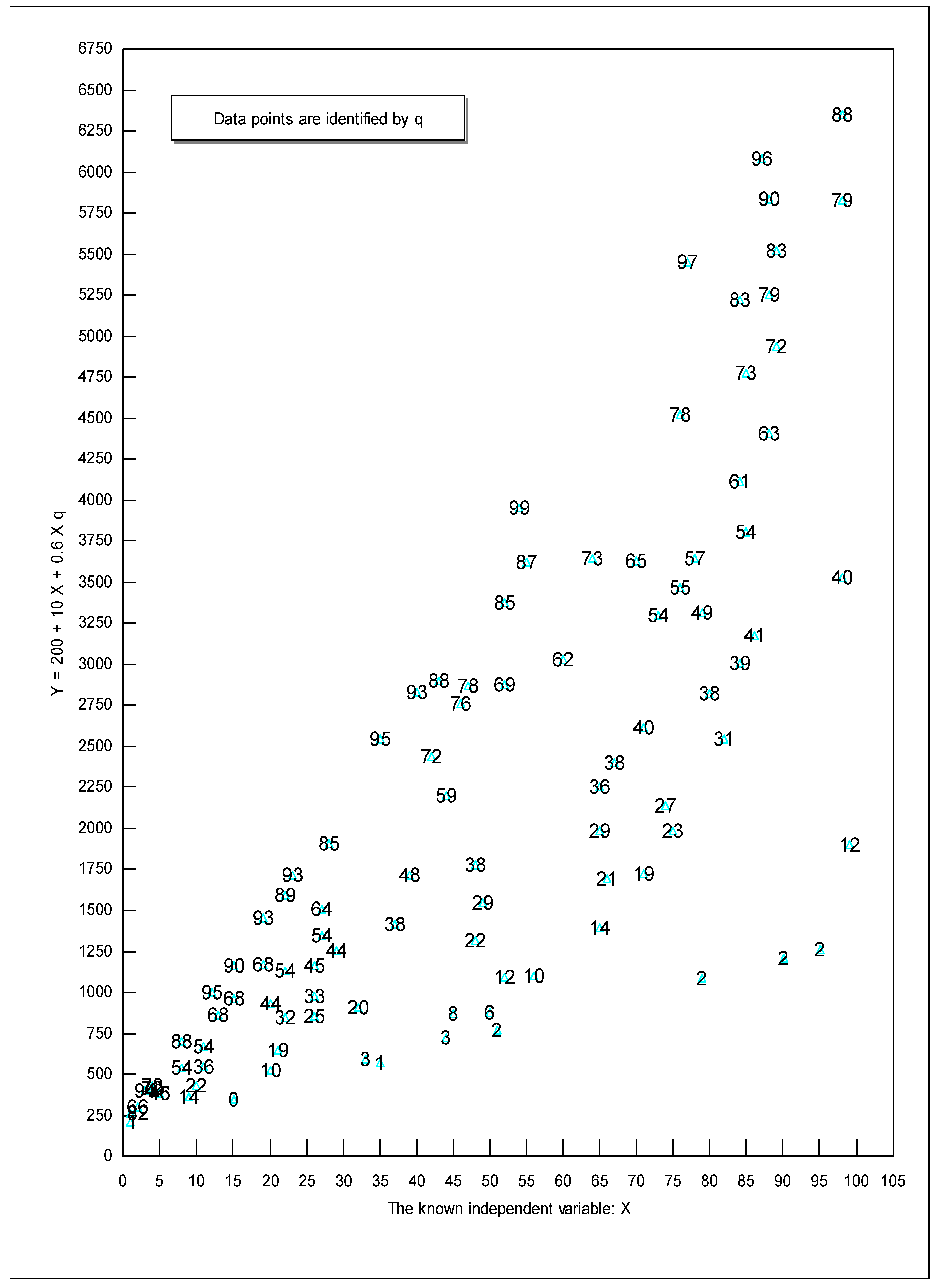
The easiest way to explain the key insight underlying variable slope estimation methods is to use a diagram like Figure 1. To construct Figure 1, we generated two series of random numbers, X and q, which ranged from 0 to 100 (for increased clarity, in this example, we set u_t = 0). We then calculated the dependent variable Y = 200 + 10 X + 0.6 q X.

The true value for dY/dX equals 10 + 0.6 q. Since q ranges from 0 to 100, the true slope will range from 10 (when q = 0) to 70 (when q = 100). Thus, q makes a 700 percent difference to the slope. In Figure 1, we identified each point with that observation’s value for q. Notice that the upper edge of the data corresponds to relatively large qs—94, 95, 95, 99, 97, 96, and 88. The lower edge of the data corresponds to relatively small qs—1, 0, 1, 2, 2, 2, and 2. This makes sense since Y increases as q increases for any given X. For example, when X approximately equals 27, reading the values of q from top to bottom of Figure 1 produces 85, 64, 54, 45, 33, and 25. Thus, the relative vertical position of each observation is directly related to the values of q. If, instead of adding 0.6qX in Equation (4), we had subtracted 0.6qX, the smallest qs would be on the top and the largest qs on the bottom of Figure 1. Either way, the relative vertical position of observations captures the influence of q. In Figure 1, the true value for dY/dX equals 10 + 0.6 q; thus, the slope, dY/dX, will be at its greatest numerical value along the upper edge of the data where q is largest and the slope will be at its smallest numerical value along the bottom edge of the data where q is smallest.

Now imagine that you do not know what q is and that you have to omit it from your analysis. In this case, OLS produces the following estimated equation: Y = 140.29 + 41.60X with an R-squared of 0.60 and a standard error of the slope of 3.44. On the surface, this OLS regression looks successful, but it is not. Remember that the true equation is Y = 100 + 10 X + 0.6 q X. Since q ranges from 0 to 100, the true slope (true derivative) ranges from 10 to 70 and OLS produced a constant slope of 41.60. OLS did the best it could, given its assumption of a constant slope; OLS produced a slope estimate of approximately 10 + 0.6 E(q) = 10 + 0.6(51.18) = 40.708 (where “E(q)” is the expected, or mean value, for q), which is close to the estimated 41.60. However, OLS is hopelessly biased by its assumption of a constant slope when, in truth, the slope is varying.

Although OLS is hopelessly biased when there are omitted variables that interact with the included variables, Figure 1 provides an important insight—even when researchers do not know what the omitted variables are, even when they have no clue how to model the omitted variables or measure the omitted variables, and even when there are no proxies for the omitted variables, Figure 1 shows researchers that the relative vertical position of each observation contains information about the combined influence of all omitted variables on the true slope. For example, if there are 500 omitted variables that increase Y and 300 that decrease Y, the observations that are on the upper frontier will correspond to when the 500 omitted variables are at their highest levels and the 300 at their lowest.

2.2. Solutions to the Omitted Variables Problem

The omitted variables problem is a well-recognized problem in regression analysis. The standard approach to solving the omitted variables problem is to find instruments to replace Z in Equation (1) so that an unbiased and consistent estimate of β₁, the partial derivative, can be estimated. However, to correctly use instrumental variables, the researcher must be able to correctly model (1) the omitted variable’s relationship with the dependent variable and (2) the relationship between the omitted variables and the instruments. Furthermore, instrumental variables must be ignorable (they do not add any explanatory value independent of their correlation with the omitted variable) and they must be so highly correlated with the omitted variable that they capture the entire effect of the omitted variable on the dependent variable. These requirements are usually impossible to meet (Bound et al. 1995) since most researchers cannot even produce a comprehensive list of all the omitted variables that could affect the true slope. Michael Murray (2017) surveyed possible strategies for dealing with cases that involve a large number of instruments and/or weakly correlated instruments.

Some researchers have used characteristics of omitted variables in order to model their influence. For example, if the omitted variables are serially correlated, then a researcher can (given some additional assumptions) use that serial correlation to account for the omitted variables (Hu et al. 2017; Arcidiacono and Miller 2011; Blevins 2016; Imai et al. 2009; Norets 2009). In contrast to using serial correlation, in this paper, we use an effect of omitted variables to capture their influence. Specifically, in this paper, we argue that omitted variables will change the relative vertical (y axis) position of observations, ceteris paribus. Using the relative position of observations, we can use our techniques from this paper with cross-sectional, time series, or panel data.

In contrast to trying to find an unbiased and consistent partial derivative, in this paper, we examine methods to find an unbiased and consistent total derivative. Thus, instead of trying to find the nonvarying β₁ of Equation (1), in this paper, we try to find the total derivative, dY/dX, of Equation (4), which equals α₁ + α₂q. When OLS is used to estimate Equation (5), instead of the true Equation (4), it produces an estimate of approximately dY/dX = α₁+ α₂E[q] which leaves an “error” for the ith observation of approximately α₂X_i(q_i − E[q]) + u_i, as shown by Equation (7).

Y = α₀ + α₁X + α₂ X{E[q] + q − E[q]} + u      adding 0 to Equation (4)

(6)

Y = α₀ + (α₁+ α₂E[q])X + α₂X(q − E[q]) + u    rearranging Equation (6)

(7)

Because this error is related to X, heteroscedasticity is a problem. Note that α₂X_i(q_i − E[q]) is the part of the error due to omitted variables and u_i is the part due to random error (measurement and round off error). We will make the typical assumption that u_i has a mean of zero. The inaccuracy for observation “i” of this dY/dX estimate will be the true slope, α₁ + α₂q_i, minus the estimated slope, α₁+ α₂E[q] as shown in Equation (8). Because this “inaccuracy” is systematic, it is a bias.

α₁ + α₂q_i − {α₁ + α₂E[q]}^ = α₂{q_i − E[q]}^ ≈ OLS inaccuracy

(8)

In this paper, we contrast the inaccuracy shown in Equation (8) with the inaccuracy from calculating an estimate of the true slope that varies from observation to observation based on Equation (13) below.

(dY/dX)^True = α₁ + α₂q      Derivative of (4)

(9)

Y/X = α₀/X + α₁ + α₂q + u/X    (4) divided by X

(10)

α₁ + α₂q = Y/X − α₀/X − u/X     (10) rearranged

(11)

(dY/dX)^True = Y/X − α₀/X − u/X   From (9) and (11)

(12)

(dY/dX)^{^} = Y/X − α₀^/X

(13)

(dY/dX)^True − (dY/dX)^{^} = (α₀^ − α₀)/X − u/X From (12) and (13)

(14)

The methods used to calculate a total derivative in this paper involve estimating α₀, the y-intercept for Equation (4). This y-intercept, Y/X, and X are plugged into the right hand side of Equation (13) to produce an estimate of dY/dX for each observation that will vary from the true value of dY/dX by an amount equal to (α₀^ − α₀)/X_i − u_i/X_i for observation i (Equation (14)). Note that, since (α₀^ − α₀)/X_i − u_i/X_i is not a systematic inaccuracy (since α₀^ − α₀ is equally likely to be positive or negative and since u_i is random), it should not be confused with a systemic bias. When Equation (4) is the true equation, but Equation (5) is used instead, this paper’s methods will produce a more accurate dY/dX for observation i than using OLS to estimate Equation (5) if |(α₀^ − α₀)/X_i − u_i/X_i| is less than |α₂{q_i − E[q]}| from Equation (8).

Let “variable slope OLS” (VSOLS) and “variable slope generalized least squares” (VSGLS) be defined as using OLS and GLS respectively to estimate α₀ from Equation (5), which is then plugged into Equation (13) along with Y and X in order to produce a separate slope estimate for each observation. The Y/X part of Equation (13) incorporates into each specific estimate its relative vertical position, which is Y/X—remember Figure 1. A.C. Aitken (1935) implies that the GLS estimate of α₀ will be the best linear unbiased estimate (BLUE) if the q_is are i.i.d. N(μ_q, σ_q²) because GLS is BLUE for heteroscedastic linear regression models. Set β₀ = α₀, β₁ = α₁+ α₂E[q] and v = α₂X(q − E[q]) + u, and substituting into Equation (7) produces2

Y = β₀ + β₁X + v where v ~N(0,σ_v²) where σ_v² = α₂² X² σ_q² + σ_u² conditionally on X.

(15)

Thus, VSGLS produces a BLUE estimate of Equation (4)’s α₀. Note that Equation (12) implies that if we can find an exact value for α₀, then we can mathematically calculate an exact value for dY/dX if all error is due to omitted variables (thus random error, u, equals 0). Therefore, if we can produce a BLUE estimate of α₀, we can mathematically calculate a BLUE estimate of dY/dX by using Equation (12) if all the error is due to omitted variables. We will examine cases where u = 0 and cases in which u ≠ 0. OLS, VSOLS, and VSGLS will be compared to reiterative truncated projected least squares (RTPLS), a technique based on DEA.

RTPLS is based on Equation (4), and the realization that the relative vertical position of each observation captures the combined influence of all omitted variables (remember Figure 1). In other words, the vertically highest observations (those at the top of a scatter plot) will be associated with values for the omitted variables that increase Y the most and the vertically lowest observations (those at the bottom) will be associated with omitted variable values that increase Y the least (Branson and Lovell 2000). RTPLS (step 1) draws an output oriented, variable returns to scale frontier around the upper left side of a scatter plot of the data in Y versus X space, (step 2) projects all the data under this frontier to that frontier (by multiplying each Y by the ratio of the distance from the x axis to the frontier that runs through a given Y divided by that Y), (step 3) truncates off any horizontal region, (step 4) runs an OLS regression through that projected data, and (step 5) associates the resulting slope estimate with the observations that determined the frontier. This slope estimate is for when q is at its most favorable level (where “favorable” means “increasing Y the most, for any given value of X”). The observations that determined the frontier are then eliminated (step 6), and the process repeated producing a slope estimate for when q is at its second most favorable level. This process is reiterated until an additional iteration would use fewer than 10 observations (step 7). Imagine this reiterative process as peeling an onion down, layer by layer, where each layer corresponds to a progressively less favorable level for q. This process contains similarities to quantile estimation except RTPLS uses the maximum number of layers possible instead of just four. Notice that Equation (13) can be rearranged as Equation (16).

(dY/dX)^ − Y/X = − α₀^_/X     (13) rearranged

(16)

A final regression (step 8) is conducted based on Equation (16) where (dY/dX)^ are the slope estimates that result from the peeling down process, (dY/dX)^ − Y/X is the dependent variable, and 1/X the sole independent variable (note: no constant is used). The α₀ estimated in this final regression along with the original data for X and Y/X are plugged into Equation (13) to calculate a separate slope estimate for each observation (step 9).

The first generation of RTPLS just peeled the data from the top; the second generation peeled the data from the top and then, restarting with the original data, peeled the data up from the bottom (using an input-oriented variable returns to scale DEA problem where the “input” is Y and the “output” is X). Peeling the data from both the top and the bottom results in approximately double the number of observations being used in the final regression and tends to increase the accuracy of RTPLS.

Leightner and Inoue (2012) compare and contrast the different generations of RTPLS and provide the math underlying the construction of (and the projection of the data to) the frontier. This open access article is available at http://www.hindawi.com/journals/ads/2012/728980/ (accessed on 1 October 2021). However, their final regression was based on Equation (13) where (dY/dX)^, the slope estimates that result from the peeling down process, is the dependent variable, and 1/X and Y/X are the independent variables (again, no constant was used). Leightner (2015) provides the most complete explanation of RTPLS published to date.

3. Results

Statistical analysis of new methods should create criteria and then compare the new methods using those criteria (Li et al. 2021; Zhang and Hong 2021). The criteria used here is minimizing the sum of the absolute value of the errors and minimizing the standard error of the errors. We generated two independent series of numbers, one for X_i and the other for q_i, both of which are uniformly distributed between 0 and 10. We then generated two sets of u_i that were normally distributed random numbers whose standard deviations were 1/100th and 1/10th of the standard deviation of the Xs. We generate each Y_i by plugging q_i, X_i, and u_i into Equation (4). We then estimate dY/dX (which equals α₁ + α₂q) by the methods described above. Our estimation techniques do not use our knowledge of q—the omitted variable; however, we can compare the estimated slopes to the true slopes since we actually do know q for each observation in our simulation context.

We ran 5000 simulations each for the 27 combinations of the omitted variable making a 10 percent, 100 percent, and 1000 percent difference to the true slope (α₁ = 1 and α₂ = 0.01, 0.1, and 1 where q ranges from 0 to 10), with the standard deviation of u = 0 percent, 1 percent, and 10 percent of the standard deviation of X, and with sample sizes of n = 100, 250, and 500.

In all the following equations, [] serves as a place holder for the different approaches analyzed: OLS, VSOLS, VSGLS, and RTPLS. “True” refers to the numerical value of the true total derivative, α₁ + α₂q, which will be different for different observations.

Table 1. The empirical results, 5000 simulations each.

	Column	1	2	3	4	5	6	7	8	9
	q’s affect	1000%	100%	10%	1000%	100%	10%	1000%	100%	10%
	size of u	0%	0%	0%	1%	1%	1%	10%	10%	10%
Panel A		mean |e|
%OLS e	n = 100	0.70887	0.17753	0.02399	0.70887	0.17753	0.02400	0.70886	0.17759	0.02499
	n = 250	0.71172	0.17706	0.02389	0.71172	0.17706	0.02389	0.71170	0.17707	0.02428
	n = 500	0.71129	0.17682	0.02386	0.71130	0.17682	0.02386	0.71131	0.17685	0.02405
Panel B
%VSOLS e	n = 100	0.57849	0.18976	0.02738	0.57733	0.18552	0.03312	0.57076	0.23972	0.32891
	n = 250	0.42280	0.11473	0.01564	0.42276	0.11507	0.03476	0.42899	0.25026	0.32705
	n = 500	0.31742	0.08605	0.01141	0.32090	0.09775	0.04337	0.36785	0.33497	0.40862
Panel C
%VSGLS e	n = 100	0.02311	0.00651	0.00089	0.02394	0.01364	0.01499	0.04773	0.10913	0.14922
	n = 250	0.01017	0.00287	0.00039	0.01179	0.01329	0.01746	0.04600	0.12690	0.17446
	n = 500	0.00544	0.00154	0.00021	0.00790	0.01410	0.01914	0.04884	0.13923	0.19137
Panel D
%RTPLS e	n = 100	0.04071	0.00795	0.00101	0.04150	0.01476	0.01489	0.06231	0.10851	0.14787
	n = 250	0.01871	0.00335	0.00043	0.02015	0.01349	0.01736	0.05073	0.12618	0.17339
	n = 500	0.01911	0.00290	0.00023	0.02076	0.01450	0.01907	0.05463	0.13874	0.19060
Panel E	standard e of |e|
%OLS error	n = 100	1.0836	0.2092	0.0275	1.0836	0.2092	0.0275	1.0836	0.2092	0.0275
	n = 250	1.0941	0.2096	0.0275	1.0941	0.2096	0.0275	1.0941	0.2096	0.0275
	n = 500	1.0947	0.2096	0.0275	1.0947	0.2096	0.0275	1.0947	0.2096	0.0275
Panel F
%VSOLS error	n = 100	3.9096	1.3301	0.1954	3.8981	1.2862	0.2085	3.8267	1.5087	2.3137
	n = 250	4.4421	1.1361	0.1535	4.4417	1.1332	0.3429	4.5118	2.4587	3.2971
	n = 500	4.6436	1.1903	0.1540	4.7211	1.4233	0.6534	5.6769	5.1948	6.1352
Panel G
%VSGLS error	n = 100	0.0714	0.0170	0.0023	0.0747	0.0378	0.0413	0.1530	0.3052	0.4118
	n = 250	0.0439	0.0107	0.0014	0.0517	0.0508	0.0657	0.1988	0.4833	0.6567
	n = 500	0.0310	0.0075	0.0010	0.0455	0.0694	0.0930	0.2709	0.6847	0.9298
Panel H
%RTPLS error	n = 100	0.1193	0.0203	0.0025	0.1224	0.0404	0.0414	0.1932	0.3065	0.4126
	n = 250	0.0749	0.0121	0.0015	0.0818	0.0516	0.0657	0.2178	0.4838	0.6571
	n = 500	0.0922	0.0127	0.0011	0.1030	0.0715	0.0930	0.3012	0.6853	0.9300
Panel I	mean |e| ratio
OLS/RTPLS	n = 100	2138.12	840.87	1062.57	117.43	31.28	3.87	28.50	3.87	0.40
	n = 250	1696.36	2496.56	4470.49	178.66	35.83	3.79	33.67	3.80	0.38
	n = 500	2729.59	3042.64	9531.99	174.76	36.27	3.79	33.80	3.79	0.38
Panel J
VSOLS/RTPLS	n = 100	660.69	236.98	247.60	29.90	7.55	1.14	7.09	1.14	0.88
	n = 250	256.71	426.66	560.03	28.55	5.49	0.96	5.17	0.96	0.86
	n = 500	316.74	319.14	862.57	19.22	3.77	0.90	3.51	0.90	0.86
Panel K
VSGLS/RTPLS	n = 100	34.11	2.76	2.63	1.57	1.00	1.02	0.95	1.02	1.02
	n = 250	2.82	3.04	2.11	1.15	1.00	1.01	0.95	1.01	1.01
	n = 500	1.63	3.18	2.15	0.68	0.98	1.01	0.92	1.01	1.01
Panel L	standard e of |e| ratio
OLS/RTPLS	n = 100	1.4025	1.4025	1.4025	1.5070	1.6937	1.7326	1.6721	1.7344	1.7446
	n = 250	1.4092	1.4092	1.4092	1.5833	1.7506	1.7563	1.7366	1.7564	1.7613
	n = 500	1.4115	1.4115	1.4115	1.5802	1.7638	1.7671	1.7484	1.7673	1.7699
Panel M
VSOLS/RTPLS	n = 100	1.3 × 10−12	1.5 × 10−12	1.5 × 10−11	0.4467	1.0568	1.2409	1.0201	1.2446	1.1031
	n = 250	9.5× 10−13	4.1× 10−12	6.3 × 10−11	0.6565	1.1906	1.2066	1.1681	1.2065	1.1056
	n = 500	1.6 × 10−12	5.0 × 10−12	1.3 × 10−10	0.6585	1.2508	1.1745	1.2307	1.1743	1.1181
Panel N
VSGLS/RTPLS	n = 100	1.5 × 10−12	1.9 × 10−12	1.8 × 10−11	0.5163	0.6732	0.3243	0.8881	0.3648	0.2952
	n = 250	2.4 × 10−12	8.1 × 10−12	9.0 × 10−11	0.7402	0.4993	0.2268	0.7798	0.2504	0.2189
	n = 500	4.3 × 10−12	1.3 × 10−11	1.8 × 10−10	0.9451	0.6504	0.1783	0.8432	0.2486	0.1758

, Panels A–D present the simulation results for the mean of the absolute value of the error as defined by Equation (18) where “n” is the number of observations in a simulation and “m” is the number of simulations. Table 1, Panels E–H present the standard deviation of these errors as defined by Equation (19) where E(E_i[]) = the mean of E_i[] = $\left({{\displaystyle \sum }}_{i=1}^n{E}_i^{[]}\right)/n$.

Define E_i[] = (estimated slope from [] − True_i)/True_i

(17)

$${{\displaystyle \sum }}_{j=1}^m[{{\displaystyle \sum }}_{i=1}^n|E_i^{\left[[]\right]}|/n]/m$$

(18)

$$\left\{{{\displaystyle \sum }}_{j=1}^M{\left[{\left({{\displaystyle \sum }}_{i=1}^n{\left(E_i^{[] }-E\left(E_i^{[]}\right)\right)}^2\right)}^{}/\left(n-1\right)\right]}^{1/2}\right\}/m$$

(19)

Panel A shows the results of using OLS to estimate Equation (5), assuming that there are no omitted variables when in truth there are. Panels B and C show the results of using VSOLS and VSGLS, respectively, to estimate α₀ and then plugging it with Y and X into Equation (13) to calculate a separate slope for each observation. Panel D shows the result of using RTPLS to estimate a separate slope for each observation.

We believe that the cases most relevant to modern day applied statistics are shown in columns 4, 5, and 6 of Table 1 where measurement and round off error (u) is one percent of the standard deviation of X. In contrast, columns 1, 2, and 3 show what happens when all the error is due to omitted variables (u = 0) and columns 7, 8, and 9 show what happens when measurement and round off error is ten percent of the standard deviation of X. Although zero and ten percent measurement and round off error are not usually reasonable in today’s world, we wanted to explore what happens at both extremes. Our analysis will start with the reasonable assumption of one percent measurement and round off error (u = 1% as shown in columns 4–6).

When u = 1%, a comparison of Panels A, C, and D reveals that VSGLS and RTPLS always had a noticeably lower mean value for |e| than OLS does no matter what the sample size and no matter what the importance of the omitted variables. Furthermore, VSGLS and RTPLS had a smaller standard error of |e| for all cases where u = 1% and the omitted variables make at least a 100% difference to the true slope (Panels E, G, and H). However, VSOLS (Panels B and F) did not perform as well as VSGLS and RTPLS.

Panels I–N explore the relative performance of different techniques in a way that incorporates an observation by observation comparison. When comparing the relative absolute value of the mean error and standard deviation of the error by observation for techniques i and j, “Ln(|E_i[i]|/| E_i[j]|)” was substituted for |E_i[]| in Equation (18) and for E_i[] in Equation (19) and then the antilog of the result was found. The natural log of the ratio of technique i’s error to technique j’s error had to be used in order to center this ratio symmetrically on the number one. Consider a two observation example where the VSGLS/RTPLS ratio is 4/1 for one observation and 1/4 for the other observation. In this example, the mean VSGLS/RTPLS ratio is 2.12 making VSGLS appear to have 2.12 times as much error as RTPLS, when (in this example) VSGLS and RTPLS are performing the same on average. Taking the natural log solves this problem. Ln(4) = 1.386 and Ln(1/4) = −1.386 and their average would be zero and the antilog of zero is 1, correctly showing that VSGLS and RTPLS are performing equally well in this example.

When u = 1%, and 250 observations are used, Panel I shows that using OLS while ignoring omitted variables produces 179 times, 36 times, and 3.8 times the mean error of RTPLS when the importance of the omitted variables are 1000%, 100%, and 10% respectively. Furthermore, Panel L shows that the standard error of |e| from using OLS while ignoring omitted variables is 1.58 times, 1.75 times, and 1.76 times the standard error of |e| when using RTPLS when 250 observations are used and the importance of the omitted variables are 1000%, 100%, and 10% respectively. Panel K shows that, when u = 1%, and the omitted variable made 100% or 10% difference to the true slope, RTPLS and VSGLS produce approximately the same mean |e|; however, Panel N shows that the standard error of |e| was less for VSGLS for these cases. When u = 1% and the omitted variable makes a 1000% difference to the true slope, then VSGLS produced 1.57 times, 1.15 times, and 0.68 times the mean error of RTPLS when 100 observations, 250 observations, and 500 observations are used respectively (Panel K, column 4).

Our primary conclusions from the cases where measurement and round off error is one percent of the standard deviation of X include the following: (1) both RTPLS and VSGLS noticeably outperform using OLS while ignoring omitted variables, (2) when the criteria is to minimize the mean |e|, RTPLS and VSGLS perform equally well except for the case when omitted variables make 1000% difference to the true slope (in this case RTPLS noticeably out-performs VSGLS with 100 observations, but VSGLS outperforms RTPLS with 500 observations), and (3) VSGLS produces a smaller standard error of the |e| for all cases.

We will now consider the extreme case when all error is due to omitted variables (u = 0). Panels A and E show that the mean of the absolute value of the error and the standard error of these errors stayed relatively constant for OLS as the sample size increases. In contrast, Panels C and G show that as the sample size increases the mean of the absolute value of the error and the standard error of these errors fell for VSGLS in columns 1 through 4 but rose in columns 5 through 9. This provides evidence that, if all “error” is due to omitted variables (or as long as random error is 1/1000th of the importance of the omitted variable), VSGLS appears to have the statistical property of consistency. However, the consistency of VSGLS is lost as random error increases.

A comparison of the numbers in Panels A-D reveals that VSGLS and RTPLS always have a noticeably lower value for the mean of the absolute value of the error than OLS and VSOLS when all “error” is due to omitted variables (columns 1–3). Columns 1–3, of Panels I, J, and K, show that VSOLS, VSGLS, and RTPLS noticeably outperform using OLS and incorrectly assuming that there are no omitted variables when all error is due to omitted variables. Column 1, Row 1 of Panel I implies that OLS produces a mean error that is 2138 times the mean error of RTPLS when 100 observations are used and all error is due to omitted variables. A comparison of the numbers in Panels I, J, and K reveals that RTPLS outperforms all other techniques when the criteria is a reduction of the mean absolute value of the error and when there is no random error (columns 1–3). For example, RTPLS produces between a half and a third of the error of VSGLS when 250 observations are used and all the error is due to omitted variables (Panel K, line 2, columns 1–3).3 When the results of columns 1–3 are considered with the results from columns 4–6, we conclude that there must be a threshold amount of measurement error and round off error between 0% and 1% where (as that error falls) RTPLS will start producing a smaller amount of mean |e| than VSGLS produces.

We will now consider the opposite extreme assumption about the size of measurement and round off error—when u = 10% of the standard deviation of X. Panel I, columns 7 and 8, reveals that as long as the importance of the omitted variable is at least ten times the size of measurement and round off error, RTPLS noticeably outperforms using OLS while ignoring omitted variables. Furthermore, Panel K, columns 7–9, reveals that VSGLS and RTPLS produce approximately the same amount of mean |e| when u = 10%. However, column 9 of Panels I and K implies that when random error is as important as the omitted variable, then using OLS while assuming that there are no omitted variables outperforms RTPLS and VSGLS. Column 9 corresponds to the case where |(α₀^– α₀)/X_i − u_i/X_i| from Equation (12) is more than |α₂{q_i − E[q]}| from Equation (8).

It is interesting to note that when q’s effect on the slope is 10 times the size of random error (columns 6 and 8) then OLS produces approximately 3.8 times the error of RTPLS; when q’s effect on the slope is 100 times the size of random error (columns 5 and 7) then OLS produces approximately 34 times the error of RTPLS.

If a researcher wants to estimate a total derivative, dY/dX, for Equation (5), which technique he or she should use depends upon the criteria and the amount of random error. If random error is 1/1000th of the importance of omitted variables or less and the researcher wants to produce the smallest mean error, then RTPLS works best. However, if the researcher wants to use the technique that produces the smallest standard error of the error, then VSGLS is best. Theoretically, VSGLS is BLUE when all error is due to omitted variables. The fact that RTPLS produces a much smaller mean error than VSGLS in this case (Panel K, columns 1–3) is probably due to RTPLS better capturing nonlinear aspects of the data. This result and reasoning are consistent with what Shaw et al. (2016) found.

It should be noted that this entire paper’s analysis was based on one known independent variable, X. However, it is easy to expand the analysis to include more than one independent variable by either adjusting Equations (12) and (13) or by purging the data of the influence of additional independent variables before conducting the analysis. For example, if α₃X₂ was added to Equation (4), then Equation (13) becomes dY/dX = Y/X − α₀/X − α₃X₂/X. In this case, the VSOLS or VSGLS estimates for α₀ and α₃ along with Y, X, and X₂ would have to be plugged into this expanded Equation (13) to calculate a separate slope estimate for each observation. Alternatively, an initial regression could be run for Y versus X and X₂, Y^ calculated as Y − α₃^X₂, and then the analysis conducted between just Y^ and X as described in this paper. This purging approach is the approach that must be taken when using RTPLS (Leightner and Inoue 2007).4

One of the major purposes of statistics is to be able to predict what will happen for the next observations. Traditional regression analysis produces dY/dX estimates that are constants for the entire population and then assumes that the next observation would have the same dY/dX. Clearly that type of reasoning does not fit VSGLS and RTPLS estimates because VSGLS and RTPLS produce a separate dY/dX estimate for every observation. However, this does not mean that VSGLS and RTPLS cannot be used to predict the value for dY/dX for the next several observations. Leightner (2015) explains how the Central limit Theorem can be used to create confidence intervals for RTPLS estimates as shown in Equation (20) (Note: Equation (20) can also be used to create confidence intervals for VSGLS estimates):

confidence interval = mean ± (s/√n)t_n−1,α/2

(20)

In Equation (20), “s” is the standard deviation, “n” is the number of observations, and t_n−1,α/2 is taken off the Student’s t table for the desired level of confidence. Here, we use the estimate for a given observation and the four estimates prior to it along with a 95% confidence level in order to create a moving confidence interval for all estimates except for the first four. The corresponding t_n−1,α/2 value is 2.776, indicating that with only four degrees of freedom (n − 1), we can be 95 percent confident that the actual mean lies within 2.776 standard deviations of the estimated mean. This 95% confidence interval also can be interpreted as meaning that there is only a five percent chance that the next RTPLS estimate will lie outside of this range if the recent variability of omitted variables does not increase (Leightner 2015)5.

4. An Example—The Spread Rate of COVID-19

For the past two years (2020 and 2021), COVID-19 has been the greatest medical and economic challenge facing the entire world. Those who make economic policy have faced and continue to face difficult decisions such as (1) to what extent should the economy be locked down to save lives while devastating the economy, (2) now that vaccinations are available, who should get them and should they be mandated, and (3) how much stimulus is needed while considering the cost of increased public debt and likely inflation? It is important that policy makers know the spread rate of COVID-19 when making these life- and economy-affecting decisions, yet the spread rate is affected by many variables which are hard to measure and, thus, are often omitted from the analysis such the degree of compliance with social distancing, wearing of masks, and quarantine regulations. Furthermore, there are countless considerations that affect the spread rate such as the density of the population, the age and general health of those exposed to the virus, and ambient air conditions. Moreover, different mutations of the virus spread at different rates and vary in terms of who they affect the most.

Here, we will use RTPLS to estimate the spread rate of COVID-19 because our simulation results imply that RTPLS is better than VSGLS (which is BLUE) when (1) there is almost no random variation and the spread of COVID-19 is due to scientific forces, not random luck, and (2) RTPLS is better at handling nonlinear relationships and the spread of a virus is not linear. Weekly data on the number of new confirmed COVID-19 cases were downloaded from the Internet (European Centre for Disease Prevention and Control 2021). We used only a week lag because the Center for Disease Control (Nishiura et al. 2020) reports that the medium incubation period for COVID-19 is four to five days (although there are cases where it lasts 14 days). Our data starts as soon as COVID-19 cases stayed above one per week. This resulted in our data starting with the week of March 30 for Brazil, March 9 for Europe and the UK, March 16 for the USA, and April 27 for South Africa. The data is presented in the left half of

Table 2. The COVID-19 data and empirical results.

Year	Week	New Cases in t					dcases in t + 1/dcases in t
		Brazil	Europe	S. Africa	UK	USA	Brazil	Europe	S. Africa	UK	USA
2020	11		20.6		3.8			2.42		5.45
2020	12		41.8		12.5	10.5		1.55		3.48	4.78
2020	13		56.8		35.6	42.1		1.18		2.22	2.36
2020	14	4.5	58.9		70.9	91.4	3.64	1.07		1.41	1.46
2020	15	8.4	54.9		91.9	125.2	2.48	1.05		1.11	1.08
2020	16	12.9	49.7		94.4	127.5	2.06	1.04		1.09	1.03
2020	17	18.7	44.0		95.3	123.4	2.00	1.11		1.07	1.04
2020	18	29.4	40.9	6.1	94.2	120.3	1.88	1.14	2.81	0.93	0.98
2020	19	47.4	38.6	9.2	79.6	109.9	1.56	1.07	2.46	0.89	0.98
2020	20	65.8	33.2	14.7	62.8	99.3	1.55	1.15	1.98	0.97	1.03
2020	21	94.3	30.1	21.2	53.2	94.7	1.45	1.22	1.74	0.90	1.05
2020	22	128.8	28.9	28.9	40.1	91.7	1.26	1.27	1.77	0.91	1.07
2020	23	154.6	28.7	43.3	28.5	90.4	1.13	1.29	1.64	1.09	1.10
2020	24	166.0	29.0	63.0	23.0	91.8	1.16	1.25	1.44	1.23	1.20
2020	25	185.0	28.2	82.6	20.3	102.3	1.25	1.23	1.49	1.26	1.42
2020	26	224.2	26.8	114.8	17.5	137.4	1.12	1.26	1.53	1.23	1.39
2020	27	243.7	25.7	167.7	13.6	183.6	1.04	1.32	1.44	1.48	1.29
2020	28	244.9	26.0	232.9	12.2	228.4	0.98	1.38	1.25	1.69	1.21
2020	29	233.0	27.8	282.6	12.6	267.3	1.15	1.55	1.04	1.66	1.08
2020	30	260.8	35.1	285.3	13.0	280.7	1.18	1.48	0.90	1.63	0.99
2020	31	298.9	43.9	248.1	13.2	270.3	1.00	1.32	0.81	1.78	0.94
2020	32	290.0	49.9	192.9	15.5	245.0	1.01	1.27	0.70	1.82	0.94
2020	33	285.3	55.3	127.9	20.3	222.1	0.97	1.25	0.72	1.47	0.93
2020	34	268.3	60.9	84.2	21.8	198.7	0.95	1.25	0.85	1.44	0.94
2020	35	245.6	68.0	63.6	23.5	179.4	1.05	1.26	0.89	1.69	1.01
2020	36	250.2	77.5	48.5	31.6	173.4	0.91	1.27	1.02	1.83	0.96
2020	37	220.2	90.8	41.7	50.0	157.9	0.91	1.25	1.11	1.54	1.06
2020	38	191.5	105.2	38.3	69.2	159.6	1.03	1.21	1.13	1.53	1.18
2020	39	189.1	119.5	35.4	97.7	179.8	0.96	1.36	1.18	1.72	1.07
2020	40	174.4	154.6	33.9	159.7	185.2	1.02	1.45	1.32	1.60	1.10
2020	41	170.6	216.0	36.6	247.9	195.6	0.93	1.43	1.25	1.33	1.18
2020	42	150.6	300.7	37.9	322.4	222.6	0.99	1.33	1.25	1.26	1.22
2020	43	140.7	392.4	39.4	396.8	263.9	1.09	1.20	1.19	1.18	1.24
2020	44	146.0	462.6	38.8	459.2	318.1	0.92	1.04	1.13	1.04	1.29
2020	45	127.0	471.0	36.1	467.5	403.5	1.24	0.94	1.35	1.07	1.39
2020	46	149.3	437.1	40.8	491.3	552.8	1.34	0.96	1.45	0.97	1.26
2020	47	191.6	411.6	51.3	470.2	687.4	1.15	0.98	1.36	0.79	1.04
2020	48	212.5	393.4	61.8	364.4	708.8	1.22	1.02	1.41	0.87	1.08
2020	49	250.3	392.6	79.1	310.3	758.3	1.14	1.02	1.66	1.12	1.16
2020	50	276.3	393.6	123.5	341.0	868.1	1.15	1.03	1.53	1.39	1.08
2020	51	310.5	395.9	181.0	465.6	932.9	0.91	0.99	1.45	1.53	0.95
2020	52	274.0	385.4	254.4	705.7	874.6	0.84	1.07	1.22	1.29	0.97
2020	53	221.2	405.6	301.5	903.1	844.5	1.41	1.04	1.26	1.22	1.18
2021	1	304.5	413.7	370.5	1091.1	988.3	1.23	0.90	1.10	1.01	1.02
2021	2	366.0	366.3	399.9	1089.0	996.4	0.97	0.92	0.78	0.78	0.88
2021	3	348.0	328.2	305.8	845.0	868.3	0.99	0.90	0.68	0.74	0.84
2021	4	337.6	289.0	199.6	618.9	719.9	0.97	0.88	0.57	0.75	0.73
2021	5	318.4	246.5	106.5	458.9	517.1	0.97	0.95	0.64	0.72	0.82
2021	6	299.9	226.2	59.9	324.6	414.8	1.04	1.06	0.91	0.73	0.88
2021	7	304.4	232.8	46.6	228.8	357.0	1.14	1.12	0.91	0.92	0.79
2021	8	338.9	252.2	34.4	203.5	275.4	1.21	1.15	1.04	0.78	0.91
2021	9	402.9	282.5	27.7	151.4	241.3	1.11	1.17	1.34	0.85	1.15
2021	10	438.8	323.1	29.0	120.3	268.8	1.09	1.18	1.30	1.02	0.96
2021	11	468.5	372.2	29.8	114.7	250.9	1.08	1.09	1.18	1.03	1.04
2021	12	495.9	396.6	27.0	109.6	252.7

, and the empirical estimates of the change in new cases of COVID-19 in time t + 1 due to a one unit increase in new cases of COVID-19 in time t [d(cases t + 1)/d(cases t)] are given in the right half of Table 2.

Table 3. 95% confidence intervals for the empirical results.

Year	Week	Brazil		Europe		S. Africa		UK		USA
		Min	Max	Min	Max	Min	Max	Min	Max	Min	Max
2020	15			0.02	2.88			−1.67	7.14
2020	16			0.64	1.71			−0.65	4.37	−1.75	6.04
2020	17			0.95	1.23			0.17	2.59	−0.02	2.81
2020	18	0.62	4.20	0.98	1.18			0.69	1.56	0.64	1.60
2020	19	1.17	2.83	0.98	1.18			0.76	1.27	0.91	1.13
2020	20	1.21	2.41	0.99	1.21			0.77	1.21	0.93	1.09
2020	21	1.10	2.28	1.00	1.28			0.77	1.14	0.93	1.11
2020	22	0.98	2.10	0.97	1.36	0.99	3.31	0.84	1.00	0.92	1.13
2020	23	0.92	1.86	0.97	1.43	1.11	2.73	0.75	1.15	0.93	1.17
2020	24	0.85	1.77	1.10	1.37	1.22	2.21	0.68	1.36	0.93	1.26
2020	25	0.94	1.56	1.18	1.32	1.24	1.99	0.66	1.49	0.79	1.55
2020	26	1.02	1.36	1.20	1.32	1.24	1.90	0.78	1.50	0.84	1.64
2020	27	0.95	1.34	1.18	1.36	1.30	1.71	0.90	1.61	0.95	1.61
2020	28	0.85	1.38	1.13	1.44	1.16	1.70	0.87	1.88	1.05	1.56
2020	29	0.85	1.37	1.03	1.66	0.84	1.85	0.93	2.00	0.93	1.63
2020	30	0.89	1.30	1.10	1.69	0.57	1.89	1.07	2.01	0.79	1.59
2020	31	0.85	1.29	1.16	1.66	0.45	1.72	1.38	1.92	0.74	1.46
2020	32	0.83	1.29	1.11	1.68	0.41	1.46	1.52	1.91	0.75	1.31
2020	33	0.82	1.30	1.04	1.71	0.49	1.18	1.33	2.01	0.82	1.13
2020	34	0.79	1.25	1.07	1.56	0.59	1.00	1.20	2.05	0.89	1.01
2020	35	0.89	1.10	1.19	1.34	0.60	0.99	1.21	2.07	0.87	1.03
2020	36	0.84	1.11	1.23	1.29	0.51	1.16	1.19	2.11	0.88	1.04
2020	37	0.81	1.10	1.22	1.28	0.54	1.30	1.19	2.00	0.85	1.12
2020	38	0.80	1.14	1.19	1.30	0.68	1.32	1.22	1.99	0.80	1.26
2020	39	0.81	1.14	1.13	1.41	0.78	1.35	1.34	1.98	0.85	1.26
2020	40	0.82	1.11	1.07	1.55	0.89	1.42	1.32	1.97	0.88	1.27
2020	41	0.83	1.11	1.07	1.60	0.98	1.41	1.20	1.89	0.98	1.26
2020	42	0.88	1.09	1.12	1.59	1.05	1.40	1.01	1.96	1.00	1.30
2020	43	0.84	1.16	1.11	1.60	1.10	1.38	0.84	1.99	0.98	1.34
2020	44	0.82	1.17	0.86	1.72	1.06	1.40	0.76	1.80	1.03	1.39
2020	45	0.71	1.36	0.69	1.69	1.03	1.44	0.86	1.48	1.06	1.47
2020	46	0.69	1.54	0.68	1.51	0.96	1.59	0.82	1.38	1.11	1.45
2020	47	0.76	1.53	0.76	1.28	0.97	1.62	0.66	1.36	0.93	1.56
2020	48	0.79	1.56	0.89	1.08	1.04	1.64	0.66	1.23	0.85	1.58
2020	49	1.02	1.41	0.90	1.07	1.13	1.76	0.63	1.30	0.84	1.53
2020	50	0.99	1.40	0.92	1.08	1.19	1.78	0.45	1.62	0.91	1.34
2020	51	0.82	1.41	0.95	1.06	1.19	1.78	0.35	1.94	0.87	1.25
2020	52	0.64	1.46	0.95	1.10	1.04	1.86	0.61	1.87	0.83	1.26
2020	53	0.52	1.65	0.96	1.10	0.96	1.89	0.92	1.70	0.81	1.33
2021	1	0.52	1.69	0.85	1.17	0.87	1.75	0.80	1.78	0.81	1.27
2021	2	0.47	1.67	0.80	1.17	0.55	1.77	0.46	1.87	0.72	1.28
2021	3	0.52	1.66	0.77	1.17	0.36	1.65	0.39	1.62	0.65	1.31
2021	4	0.62	1.61	0.77	1.09	0.16	1.60	0.39	1.41	0.50	1.36
2021	5	0.74	1.31	0.85	0.97	0.24	1.27	0.51	1.09	0.60	1.12
2021	6	0.91	1.07	0.76	1.12	0.39	1.05	0.69	0.80	0.68	0.98
2021	7	0.84	1.20	0.73	1.24	0.35	1.14	0.57	0.98	0.67	0.95
2021	8	0.80	1.34	0.75	1.32	0.32	1.31	0.58	0.99	0.65	1.00
2021	9	0.86	1.33	0.87	1.31	0.34	1.59	0.59	1.01	0.56	1.26
2021	10	0.96	1.28	1.02	1.25	0.58	1.61	0.58	1.15	0.61	1.27
2021	11	0.99	1.26	1.05	1.24	0.70	1.60	0.66	1.18	0.64	1.30

presents the moving 95% confidence intervals for the estimates.

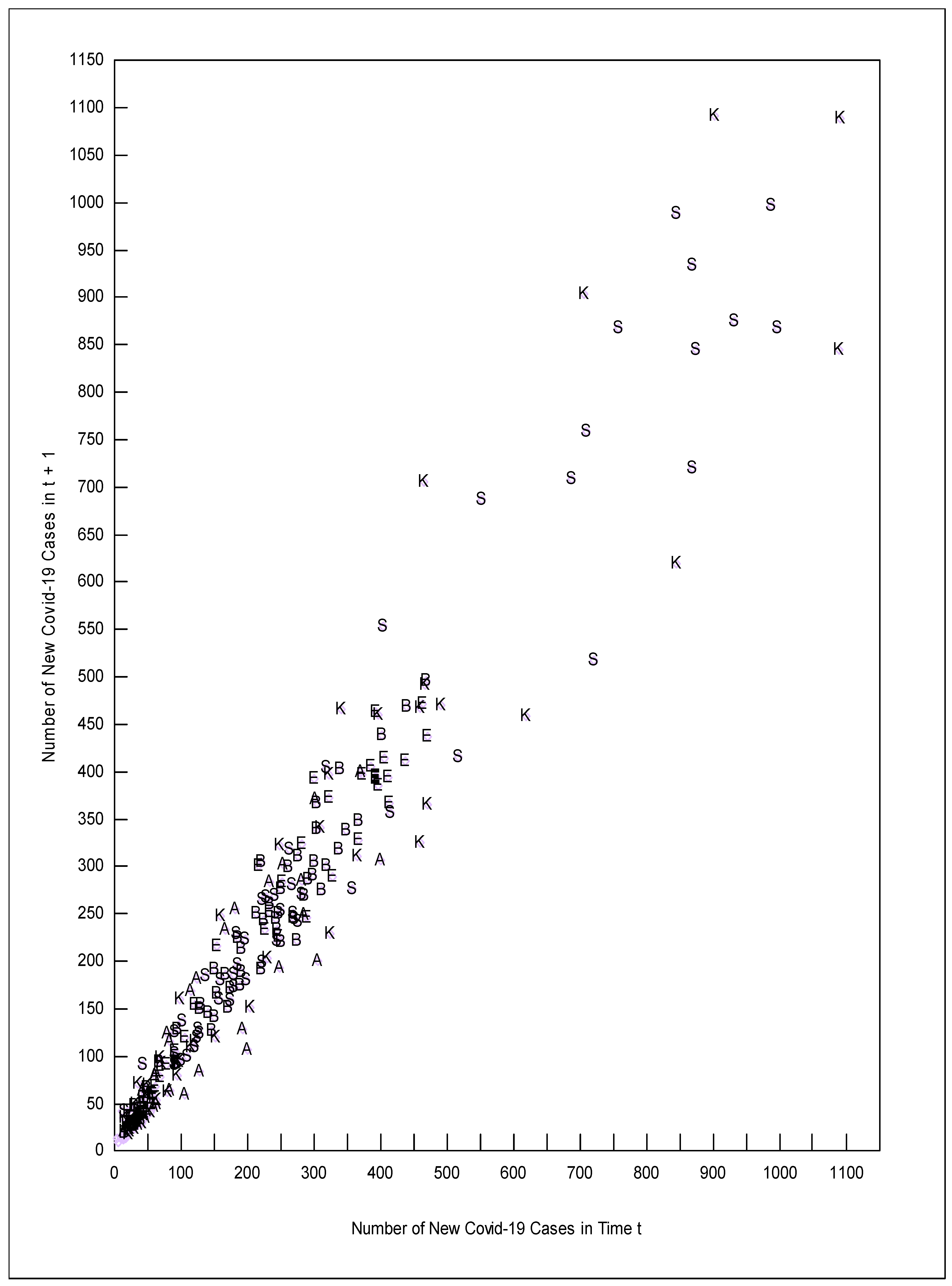
In Figure 2, the new cases of COVID-19 in time period t + 1 are plotted on the y axis versus the number of new cases of COVID-19 in time period t on the x-axis. The points on Figure 2 are identified by a letter for each country: B = Brazil, E = Europe, A = South Africa, K = The United Kingdom, and S = the USA. The shape of the range that the observations created in Figure 2 looks similar to the shape of the range of observations in Figure 1. We ran the analysis using the data shown in Table 2 and also using the natural log of the data in Table 2 (for which the slopes would then be spread elasticities). We chose to focus the analysis on the data that were not logged specifically because the non-logged data look like Figure 1, and the logged data do not.

Figure 2 shows that the UK and the USA suffered from the highest levels of new cases of COVID-19 (the upper right hand quadrant of Figure 2 contains only K and S markers indicating the UK and the USA respectfully). It is interesting that the lower right frontier of the data contains observations from South Africa (A), the United Kingdom (K), and the USA (S) and these same countries are also on the upper left hand frontier. Brazil and Europe observations (B and E) are concentrated in the middle of the data through the upper left frontier. This spread of a given country’s observations between the upper left and lower right frontiers implies that omitted variables within a given country are affecting where observations lie, instead of differences in the situation between countries. A fixed effects regression model would be inappropriate in this situation. The equation underlying the RTPLS process used in this paper was Equation (4) where Y = the number of new cases in t + 1, X = the number of new cases in t, and q is the combined effect of all omitted variables. The omitted variables within a country would include the spread of mutant variants of the virus and where it was spreading, the percent of the population vaccinated and who was vaccinated, changes in climate, changes in the enforcement and adherence to social distancing rules, etc.

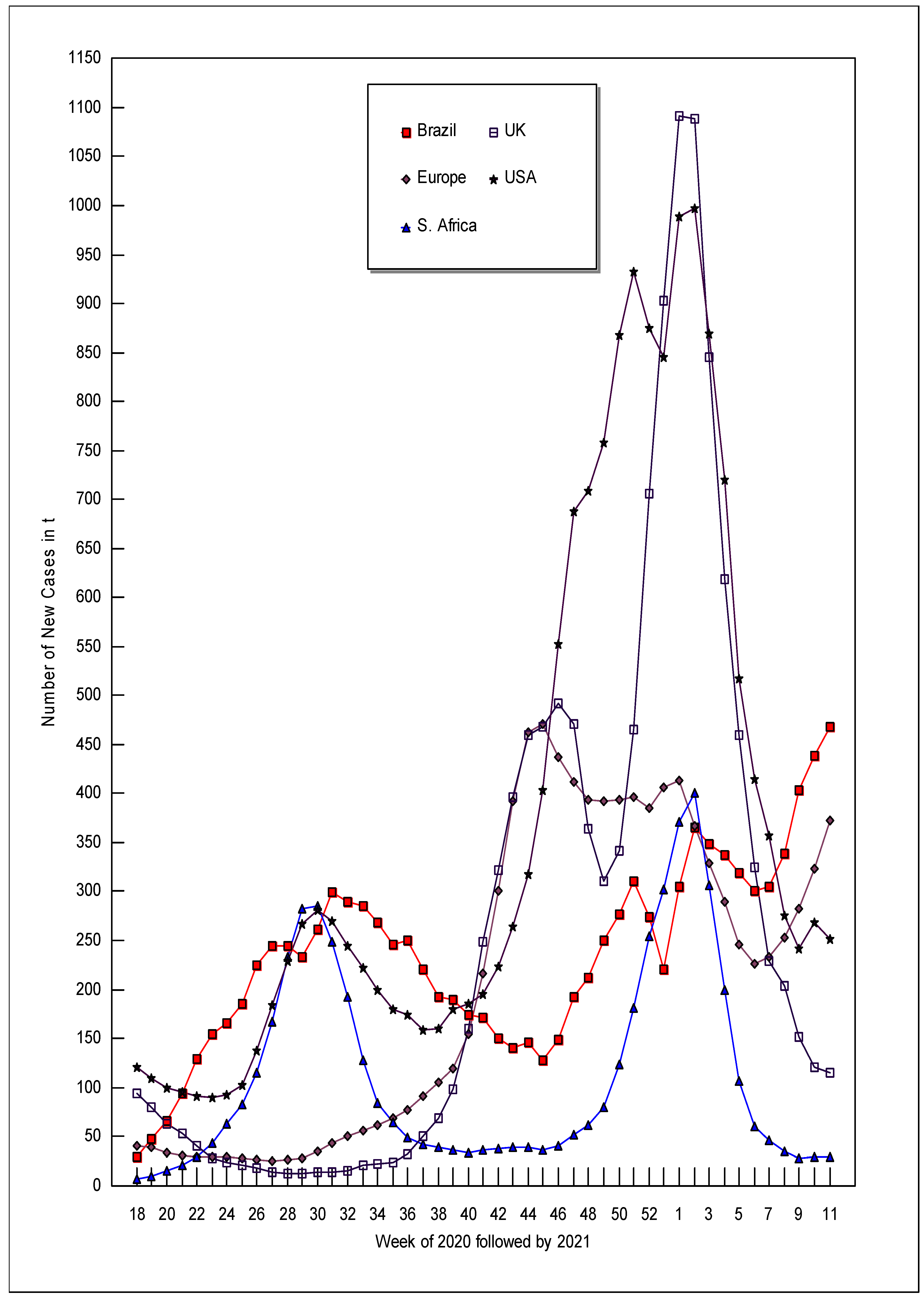
In Figure 3, we plot the spread of COVID-19 over time for each country starting with the week of April 27 (week 18). The large surges of new COVID-19 cases that occur in the middle of Figure 3 correspond to weeks soon after new COVID-19 variants are discovered. COVID-19 variant B.1.1.7 originated in the United Kingdom by September 2020, and Figure 3 shows that the largest upsurge of COVID-19 cases in the UK began in the middle of September 2020 (weeks 38 and 39). COVID-19 variant B.1.351 emerged in South Africa by the beginning of October 2020 (week 41), and South Africa’s biggest upsurge in new cases occurred approximately six weeks later (week 47). It is not known when COVID-19 variant P.1 started in Brazil, but the variant was well established by late December 2020 (week 53); Brazil’s largest upsurge of new cases of COVID-19 occurred between 2 November (week 45 of 2020) and 11 January 2021 (week 2 of 2021) (Center for Disease Control and Prevention 2021). The delta variant emerged after this paper’s data were collected.

Figure 3 also shows that the number of new cases of COVID-19 fell for all the analyzed countries between 10 January (week 2) and 14 February 2021 (week 6). During these five weeks, Brazil went from zero percent vaccinated to 2.46, Europe went from 0.6 percent vaccinated to 5.02, the UK went from 3.94 percent vaccinated to 23.33, and the USA went from 2.69 percent vaccinated to 15.81. To the extent that countries vaccinated their most vulnerable populations first, the first vaccinations would have the greatest effect.

However, more factors than just vaccinations are probably involved in the fall of new cases in early 2021 as evidenced by South Africa. New cases fell in South Africa between 10 January and 28 February 2021 despite South Africa not yet vaccinating at that time. January and February are in South Africa’s summer, and COVID-19 spreads best in low temperatures and low humidities. Anne Soy (2020) argues that Africa in general had lower COVID-19 deaths due to quicker action, stricter restrictions, greater public support, younger populations with few old age homes, favorable climates, and good community health centers. She cites South Africa in particular as having “one of the most stringent lockdowns in the world”, which resulted in the loss of 2.2 million jobs in the first half of 2020.

The fall in new cases of COVID-19 continued through 30 March for South Africa, the United Kingdom, and the USA. New cases in the UK, which had a higher peak of new cases of COVID-19 in the first week of January 2021 (1091 new cases) than the USA had (988 new cases), fell noticeably lower than the USA new cases by 30 March 2021 (UK = 110 new cases, the USA = 253 new cases). This difference could be cited as evidence that the UK’s policy of giving each citizen one shot prior to giving anyone two shots was more effective than the US policy of fully vaccinating people (requiring two shots) as soon as possible.

Figure 3 also shows that Europe and Brazil suffered from a resurgence of new COVID-19 cases starting the week of 7 February 2021, which could reflect their slower vaccination rates. By 30 March 2021, Europe had vaccinated only 16.43 percent of its population and Brazil had only vaccinated 8.57 percent of its population in contrast to the UK’s 50.85 percent and the USA’s 44.13. As of 30 March 2021, it appears that mutant virus strains are spreading faster than the relative slow vaccination programs of Brazil and Europe can contain them; however, the more rapid vaccination programs in the UK and the USA are reducing the spread of COVID-19 and its mutant variants. New cases in South Africa continue to fall despite South Africa having the lowest vaccination rates of the countries examined.

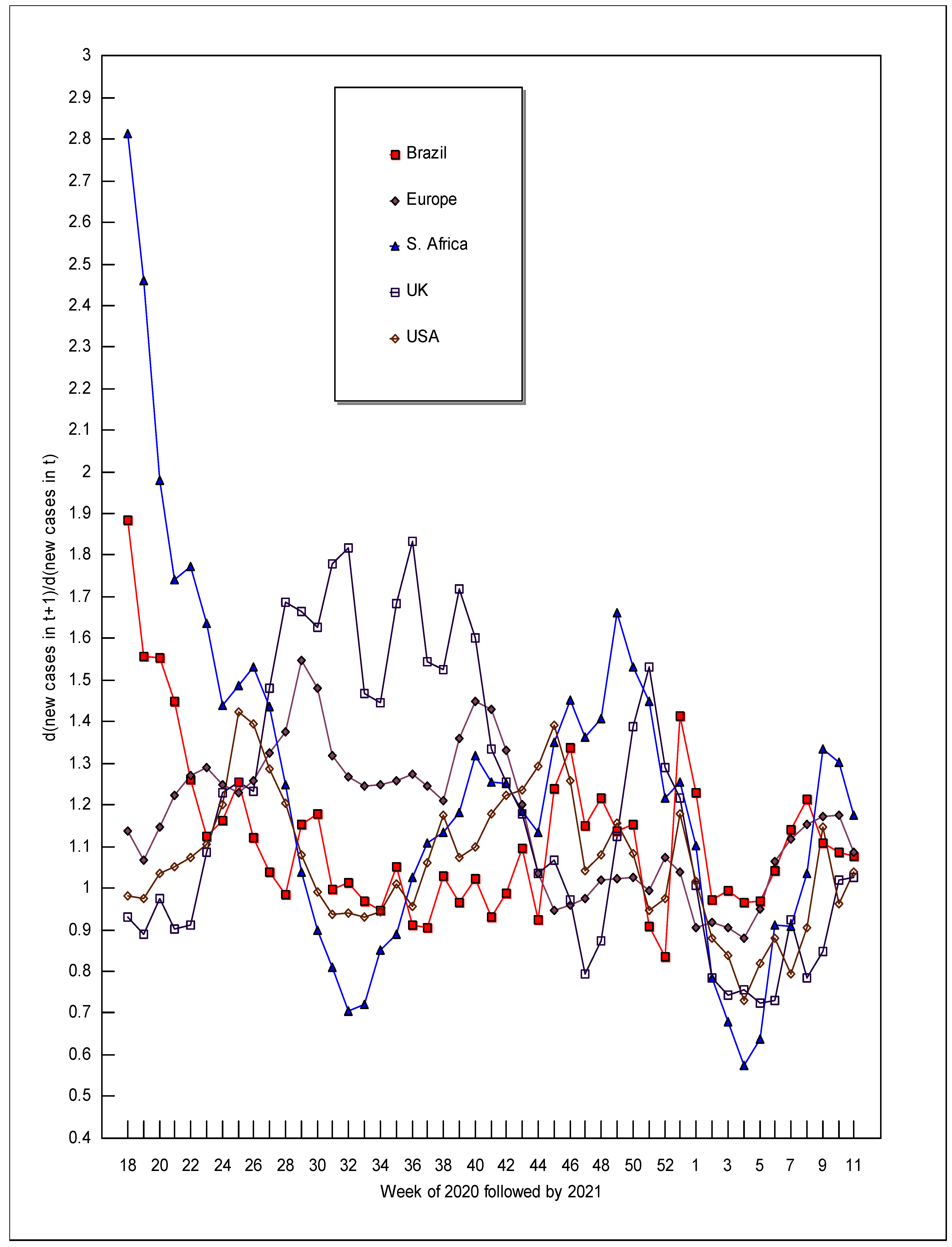
The right half of Table 2 gives the RTPLS estimates for d(new cases of COVID-19 in time t + 1)/d(new cases of COVID-19 in time t), or “dcases t + 1/dcases t” and Figure 4 plots those estimates over time. When COVID-19 first entered a country in 2020, the numerical values of dcases t + 1/dcases t were relatively high: 3.64 for Brazil (in week 14), 2.42 for Europe (week 11), 2.81 for South Africa (week 18), 5.45 for the UK (week 11), and 4.78 for the USA (week 12). The dcases t + 1/dcases t of 3.64 for Brazil in week 14 of 2020 means that an additional new case of COVID-19 in that week would have been correlated with an additional 3.64 new cases a week later (week 15). The 3.64 new cases in week 15 would then be correlated with 9.03 new cases in week 16 (3.64 times week 15′s dcases t + 1/dcases t of 2.48). This multiplicative effect causes new viruses to spread at an exponential rate (Sharma et al. 2021).

It is important to realize that the dcases t + 1/dcases t values in Table 2 and depicted in Figure 4 are total derivatives, not partial derivatives. In other words, the numerical values for dcases t + 1/dcases t show the effects of all the ways that new COVID-19 cases in t + 1 are related to new COVID-19 cases in t. For example, these values would include the effects of new mutations of the virus, of changes in weather, of changes in social distancing measures, and of changes due to vaccinations, etc. Some of these included forces would increase the spread rate (such as mutations) and others would decrease the spread rate (such as vaccinations). A partial derivative obtained from traditional regression analysis would hold all of these other forces constant; however, health officials need to know the spread rate holding nothing constant, which is what we report in this paper.

The dcases t + 1/dcases t estimates apply to both increases and decreases of new cases of COVID-19. For example, consider the first weeks of 2021 for Brazil. New cases went from 304.5 (week 1) to 366.0 (week 2) to 348.0 (week 3); meanwhile, the corresponding values for dcases t + 1/dcases t were 1.23 (week 1) and 0.97 (week 2). This means not only that an additional case of COVID-19 in week 1 was correlated with an increase of 1.23 new cases in week 2 but also that if there was one fewer new case in week 2, then the number of new cases in week 3 would decline by only 0.97 cases. What would be best for humanity is for the dcases t + 1/dcases t values to always be less than one for increases in new cases and greater than one for decreases in new cases. Unfortunately, that is not the case. Instead, every single instance in Table 2 where dcases t + 1/dcases t was less than one corresponds to falls in new cases. Likewise increases in new cases are always associated with dcases t + 1/dcases t values that are greater than one (however, there are a few cases where declines in new cases correspond to dcases t + 1/dcases t being greater than one—for example, South Africa in week 36 of 2020). This means that if new cases increase in one week, perhaps due to people not wearing their masks, then to undo the damage caused, cases in the next week would have to fall by more than they rose in the previous week.

Figure 4 reveals several interesting patterns in the dcases t + 1/dcases t estimates. First, these estimates are not random over time; in other words, although the estimates do flucuate between time t and t + 1, they do not fluctuate from the top of the graph to the bottom of the graph from time t to time t + 1 (in contrast to what our randomly generated simulation data would have shown). Second, there is a general downward trend in the estimates, which is good news for humanity. Third, the UK and Europe wander around a similar path while the USA, Brazil, and South Africa wander around a noticeably different path. The two paths converging and falling together in early 2021 can be explained by the advent of vaccines, which tended to be given to the most vulnerable people first (except for South Africa’s fall, as discussed above).

The confidence intervals reported in Table 3 vary noticeably in width; during times of relatively stable spread rates, these confidence intervals shrink and then expand when variability increases. These confidence intervals were wide when COVID-19 first hit a country and when new variants of the virus first emerged. All of the estimates reported in Table 2 fall within the 95% confidence intervals reported in Table 3. The estimates presented in this paper, the trajectory of these estimates, and their confidence intervals can help governments and their health officials predict the future course of COVID-19, making it possible for them to make better informed choices concerning lockdowns, vaccine mandates, and economic stimulus.

5. Conclusions

There are many times when decision makers need to understand the effects of their policies, but using traditional regression methods is not viable because (1) an adequate model would be too complex and would require data that is not available, (2) the time period for which there is data would be too short, and (3) an assumption that there are no omitted variables is not reasonable. In this paper, we propose several methods of producing a separate total derivative for each observation where the differences in these total derivatives are due to omitted variables. The data requirements for using these methods are minimal, and simulations show that using these methods is much better than just assuming that there are no omitted variables when there really are. We conclude that these methods, especially variable slope generalized least squares (VSGLS) and reiterative truncated projected least squares (RTPLS), are worthy of additional study.

Although we focused on cases where there are systems of equations that interact, the techniques explained here also work when omitted variables are a problem for the estimation of single equations. Since the vast majority of studies that use regression analysis can be criticized for omitted variables that could affect the slope, the techniques explained in this paper have almost unlimited applicability.

The contributions of this paper to the literature include the following: (1) this is the first paper to compare and contrast the performance of VSOLS, VSGLS, and RTPLS using simulations; (2) this is the first paper to show how our way of modeling the omitted variables problem fits with the classic way of modeling this problem and improves upon the classic approach; and (3) this is the first paper to apply a variable slopes estimation process to the spread of an infectious disease. One of the most disturbing policy implications of our COVID-19 example is that a one-person increase in new COVID-19 cases this week will cause new cases of COVID-19 to increase by more than one person next week; in contrast, a one-person decrease in new COVID-19 cases this week will reduce new cases next week by less than a whole person. Ceteris paribus, this result provides additional support for those who want stronger economic lockdowns, mandated vaccinations, and quarantines.

References

- Aitken, Alexander Craig. 1935. On Least Squares and Linear Combinations of Observations. Proceedings of the Royal Society of Edinburgh 55: 42–48. [Google Scholar] [CrossRef]
- Arcidiacono, Peter, and Robert Miller. 2011. Conditional Choice Probability Estimation of Dynamic Discrete Choice Models with Unobserved Heterogeneity. Econometrica 79: 1823–67. [Google Scholar]
- Blevins, Jason. 2016. Sequential Monte Carlo Methods for Estimating Dynamic Microeconomic Models. Journal of Applied Econometrics 31: 773–804. [Google Scholar] [CrossRef] [Green Version]
- Bound, John, David A. Jaeger, and Regina M. Baker. 1995. Problems with Instrumental Variables Estimation when the Correlation between the Instruments and the Endogenous Explanatory Variable is Weak. Journal of the American Statistical Association 90: 443–50. [Google Scholar] [CrossRef]
- Branson, Johannah, and Charles Albert (Knox) Lovell. 2000. Taxation and Economic Growth in New Zealand. In Taxation and the Limits of Government. Edited by Gerald W. Scully and Patrick James Caragata. Boston: Kluwer Academic, pp. 37–88. [Google Scholar]
- Center for Disease Control and Prevention. 2021. Science Brief: Emerging SARS-CoV2 Variants. Available online: https://www.cdc.gov/coronavirus/2019-ncov/science/science-briefs/scientific-brief-emerging-variants.html?CDC_AA_refVal=https%3A%2F%2Fwww.cdc.gov%2Fcoronavirus%2F2019-ncov%2Fmore%2Fscience-and-research%2Fscientific-brief-emerging-variants.html (accessed on 15 April 2021).
- Dulaney, Chelsey. 2017. Dollar Kicks off the New Year on a High Note. The Wall Street Journal, January 4, B16. [Google Scholar]
- European Centre for Disease Prevention and Control. 2021. COVID-19 Update Situation, Worldwide. Available online: https://www.ecdc.europa.eu/en/geographical-distribution-2019-ncov-cases (accessed on 18 September 2021).
- Hu, Yingyao, Matthew Shum, Wei Tan, and Ruli Xiao. 2017. A Simple Estimator for Dynamic Models with Serially Correlated Unobservables. Journal of Econometric Methods, 1–16. [Google Scholar] [CrossRef] [Green Version]
- Imai, Susumu, Neelam Jain, and Andrew Ching. 2009. Bayesian Estimation of Dynamic Discrete Choice Models. Econometrica 77: 1865–99. [Google Scholar]
- Leightner, Jonathan E. 2015. The Limits of Fiscal, Monetary, and Trade Policies: International Comparisons and Solutions. Singapore: World Scientific. [Google Scholar]
- Leightner, Jonathan E. 2020. Estimates of the Inflation versus Unemployment Tradeoff that are not Model Dependent. Journal of Central Banking Theory and Practice 2020: 5–21. [Google Scholar] [CrossRef] [Green Version]
- Leightner, Jonathan E., and Tomoo Inoue. 2007. Tackling the Omitted Variables Problem without the Strong Assumptions of Proxies. European Journal of Operational Research 178: 819–40. [Google Scholar] [CrossRef]
- Leightner, Jonathan E., and Tomoo Inoue. 2008. Capturing Climate’s Effect on Pollution Abatement with an Improved Solution to the Omitted Variables Problem. European Journal of Operational Research 191: 539–56. [Google Scholar] [CrossRef]
- Leightner, Jonathan E., and Tomoo Inoue. 2012. Solving the Omitted Variables Problem of Regression Analysis using the Relative Vertical Position of Observations. Advances in Decision Sciences. Available online: http://www.hindawi.com/journals/ads/2012/728980/ (accessed on 1 October 2021).
- Li, Ming-Wei, Yu-Tain Wang, Jing Geng, and Wei-Chiang Hong. 2021. Chaos cloud quantum bat hybrid optimization algorithm. Nonlinear Dynamics 103: 1167–93. [Google Scholar] [CrossRef]
- Murray, Michael P. 2017. Linear Model IV Estimation when Instruments are Many or Weak. Journal of Econometric Methods De Gruyter 6: 1–22. [Google Scholar] [CrossRef]
- Nishiura, Hiroshi, Natalie Linton, and Andrei Akhmetzhanov. 2020. Serial interval of novel coronavirus (COVID-19) infections. International Journal of Infectious Diseases 93: 284–86. [Google Scholar] [CrossRef] [PubMed]
- Nizalova, Olena Y., and Irina Murtazashvili. 2016. Exogenous Treatment and Endogenous Factors: Vanishing of Omitted Variable Bias on the Interaction Term. Journal of Econometric Methods De Gruyter 5: 71–78. [Google Scholar] [CrossRef]
- Norets, Andriy. 2009. Inference in dynamic discrete choice models with serially correlated unobserved state variables. Econometrica 77: 1665–82. [Google Scholar]
- Ramsey, James Benard. 1969. Tests for Specification Errors in Classical Linear Least-Squares Regression Analysis. Journal of the Royal Statistical Society, Series B (Methodology) 31: 350–71. [Google Scholar] [CrossRef]
- Sharma, Sunil Kumar, Aashima Bangia, Mohammed Alshehri, and Rashmi Bhardwaj. 2021. Nonlinear Dynamics for the spread of Pathogenesis of COVID-19 Pandemic. Journal of Infection and Public Health 14: 817–31. [Google Scholar] [CrossRef] [PubMed]
- Shaw, Philip, Michael Andrew Cohen, and Tao Chen. 2016. Nonparametric Instrumental Variable Estimation in Practice. Journal of Econometric Methods 5: 153–78. [Google Scholar] [CrossRef] [Green Version]
- Soy, Anne. 2020. Coronavirus in Africa: Five Reasons Why COVID-19 Has Been Less Deadly than Elsewhere. BBC News. October 8. Available online: https://www.bbc.com/news/world-africa-54418613 (accessed on 21 April 2021).
- Zhang, Zichen, and Wei-Chiang Hong. 2021. Application of variational mode decomposition and chaotic grey wolf optimizer with support vector regression for forecasting electric loads. Knowledge-Based Systems 228: 107297. [Google Scholar] [CrossRef]
Figure 1.
The intuition underlying variable slope estimators.
Figure 2.
New cases of COVID-19 in t + 1 (y axis) versus new cases in t (x axis). A = South Africa, B = Brazil, E = Europe, K = United Kingdom, S = USA.
Figure 3.
New cases of COVID-19 over time.
Figure 4.
The change in d(new cases t + 1)d(new cases t) over time.