A Novel Model Structured on Predictive Churn Methods in a Banking Organization

Abstract

A constant in the business world is the frequent movement of customers joining or abandoning companies’ services and products. The customer is one of the company’s most important assets. Reducing the customer abandonment rate has become a matter of survival and, at the same time, the most efficient way to maintain the customer base, since the replacement of dropouts by new customers costs, on average, 40% more. Aiming to mitigate the churn (customer evasion) phenomenon, this study compared predictive models to discover the most efficient method to identify customers who tend to drop out in the context of a banking organization. A literature review of related works on the subject found the neural network, decision tree, random forest and logistic regression models were the most cited, and thus the models were chosen for this work. Quantitative analyses were carried out on a sample of 200,000 credit operations, with 497 explanatory variables. The statistical treatment of the data and the developments of predictive models of churn were performed using the Orange data mining software. The most expressive results were achieved using the random forest model, with an accuracy of 82%.

1. Introduction

The behavior of consumers and their relationships with companies are being affected by the profound changes brought about by access to and speed of information, technological advances, and fierce competitiveness, making them more demanding and less loyal to companies.

Successful companies have satisfactory and long-term relationships with their customers (Zhu et al. 2017), allowing the institution to focus its efforts on the customer’s needs and opening up new service possibilities (Mehta et al. 2016). Searching for new customers is an essential activity for companies, but more costly than maintaining a relationship with an existing customer. Higher attrition rates typically characterize new customers. In return, a satisfied customer indicates and recommends the company to other potential customers (Depren 2018).

Keeping a customer cost approximately five times less than acquiring a new one (He et al. 2014). According to Reichheld and Sasser (1990), in the case of bank branches, a study showed that a 5% reduction in the abandonment rate—a metric that indicates how much your company has lost in revenue or customers—is capable of increasing profits by 85%. Analyzing customer behavior enables strategies that can be used for retention; however, this activity is a task that requires the analysis of large volumes of data. Tools like data mining can help the company to understand the customer’s need according to what it can offer.

Data mining is a technique to extract data from the histories stored in computational devices, analyze them, and transform them into useful information, with the objective of more accurate strategic decision-making (Steiner et al. 1999). Data mining technology can detect important clues behind large amounts of available information, enabling the creation of a predictive model of customer churn.

CRM emerged as an essential tool to win and increase customer loyalty and has become necessary, considering the increasingly different demands on companies. With the use of information technology, CRM started to be used as a strategic tool to maintain and improve the relationship with the customer and, mainly, prevent them switching to a competitor.

‘Churn’ is customers’ action in giving up operating with a company and migrating to its competitors (Ghorbani and Taghiyareh 2009). The loss of clientele is an increasing concern and must be addressed as a priority by organizations, as it can impact revenue and, consequently, companies’ survival.

The retention rate is represented by the number of customers who remain with the company, calculated on the entire (Jahanzeb and Jabeen 2007) customer base. The churn rate can be extracted as follows:

$$\mathrm{Churn}\mathrm{rate}=\frac{C_0+A_1-C_1}{C_0}$$

(1)

• C₀—number of customers at the beginning of the period
• A₁—new customers who joined in the given period
• C₁—number of customers at the end of the period.

To handle and manage the churn rate, it is essential to create a predictive model. In most cases, the techniques are based on the client’s history, through variables with greater influences on the churn phenomenon. The models analyze, identify, and classify each customer’s probabilities of evasion, individually, aiming at customer retention measures (Idris et al. 2012).

Effective predictive models analyze customer history through a mass of data extracted from the computing devices that support the applications used by customers.

This data undergoes mining that transforms it into relevant information, identifying customer behavior and enabling decision making (Adebiyi et al. 2016).

This article aims to compare the four main machine learning algorithms according to the literature to find the best predictive churn model to address preventively customer evasions in a banking organization.

In Section 2, the most popular algorithms in predictive churn models will be shown through bibliometric research. In Section 3, the processes of the CRISP-DM methodology for the construction of the model will be described. Section 4 will outline the results obtained and, finally, Section 5, Section 6, Section 7 and Section 8 will report the discussions, conclusions, limitations of the article, and suggestions for future work, respectively.

2. Materials and Methods

To investigate the current state of research on churn predictive models, a literature review was performed. This approach makes it possible to provide an overview of previous research on the subject and a holistic perspective on the common knowledge bases. In addition, the review contributes to the development of the machine learning field concerning predictive models, identifying different research streams with different approaches, and using the most varied algorithms. A review approach is characterized by thoroughness and rigor, leading to the legitimacy and objectivity of the results (Creswell and Creswell 2017; Jesson et al. 2011; Tranfield et al. 2003).

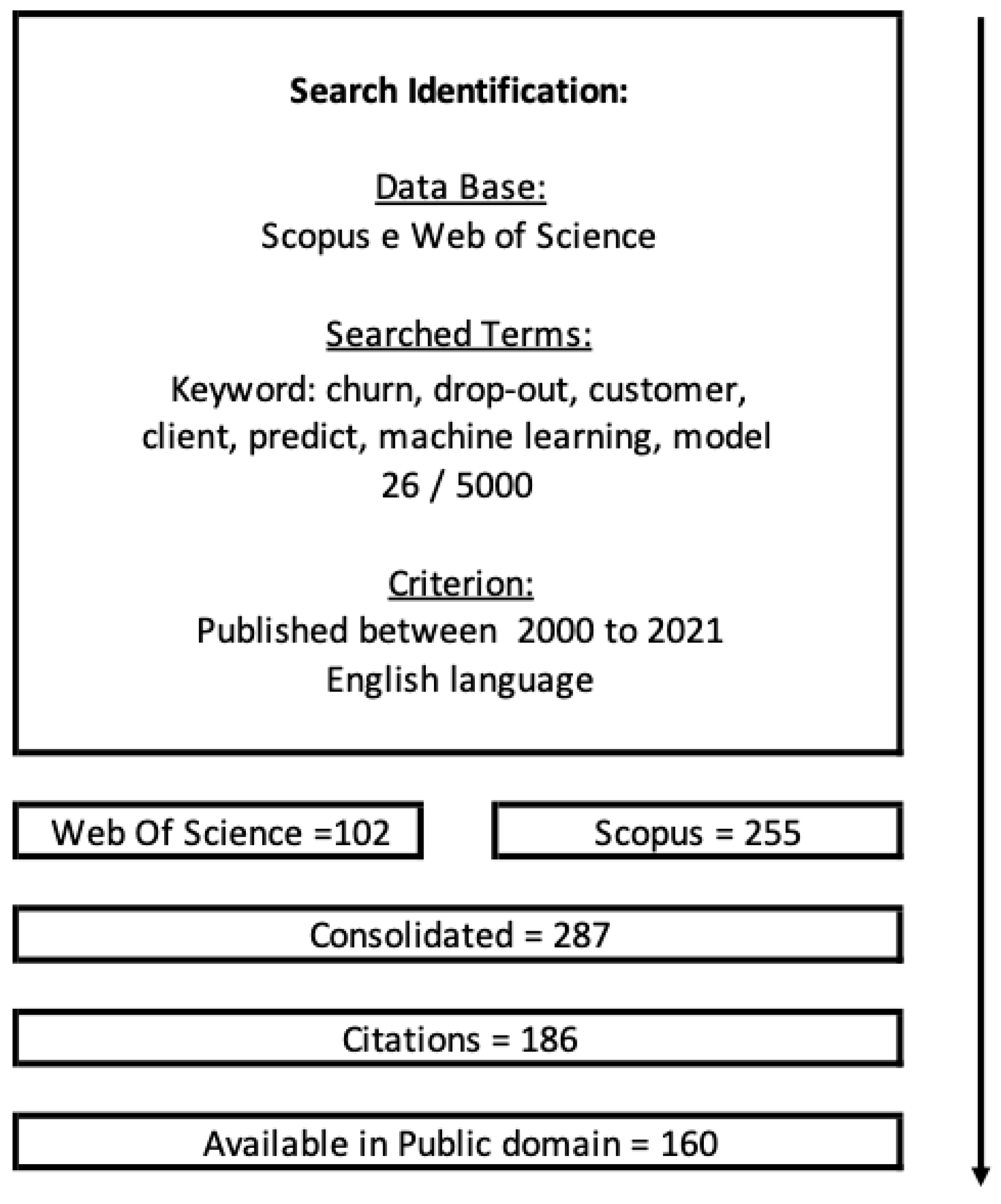
As shown in Figure 1, in a first step, the research field was accessed, obtaining an overview of the relevant works in the field of machine learning that deals with the churn phenomenon. The objective was to identify articles from relevant journals referring to churn predictive models.

To be included in the review, the title or keywords of an article should contain the string: (“churn*”) AND (“customer*” OR “client*”) AND (“predict* OR “machine learning*” OR “model*”). The terms were connected using Boolean logic, a method by which the database can search for certain combinations of keywords. Using an asterisk with the search term ensured that variations (e.g., client and clients or model and modeling, or predict and prediction) were included in the results of the bibliographic searches. As an additional inclusion criterion, the type of publication was defined as a journal article, in English and published between 2000, when the study of the topic began, until 2021.

A search in the Web of Science (WoS) indexing database resulted in 288 published articles. After applying the refinement to the category “Computer Science Artificial Intelligence”, the result dropped to 102 articles.

The same query was performed on the SCOPUS indexing base, returning 276 published articles. After refining the subject area to “Computer Science”, the result reduced to 225 articles.

A further refinement was performed, removing all articles that were not cited as references by any other research, leaving 186 articles.

For the 186 articles, only 160 documents were publicly available, which served as a basis for pre-processing, and they were submitted for further refinement to group related terms.

To identify the most recurrent predictive models in these publications, we chose to use a bibliometric analysis of the texts. According to Pritchard (1969), bibliometrics can be defined as the application of statistical and mathematical methods to books and other media, with its focus on measuring the tangible output of scientists through books, articles, patents, and others.

The analysis of terms was performed with the support of software called VOSviewer, which is a tool for building and viewing bibliometric networks. It allows the creation of networks 107 of citation relationships, bibliographic coupling, co-citation, or co-authorship (Van Eck and Waltman 2010).

VOSviewer is also a tool we have developed over the past few years that relatively easily provides the basic functionality needed to view bibliometric networks (Van Eck and Waltman 2014).

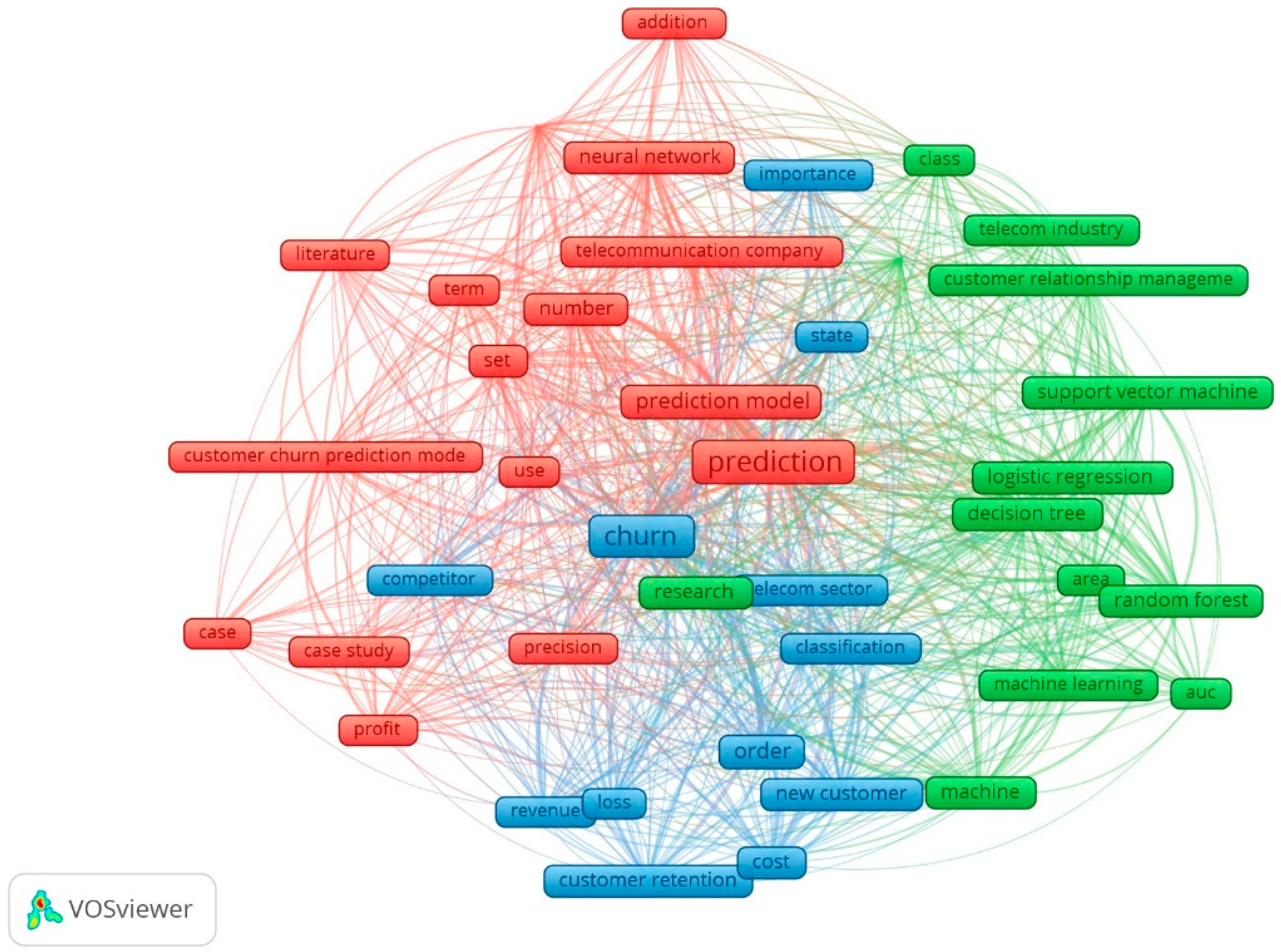
Keywords are nouns or phrases that reflect the core content of a publication. Content is studied through keyword distribution analysis. Bibliometric data showed that there were 3174 terms, however, only terms that appeared at least ten times in the analyzed texts were selected, returning 69 keywords, and of these, only 60% (41 terms) were selected. As can be seen in Figure 2, in the network, the view items are represented by their label and a circle. The item’s weight determined the label size and circle of an item. The more significant the weight of an item, the larger (Yang et al. 2017) the item label and circle will be. In this study, the software identified three clusters, composed of terms that tend to be mentioned together. To choose the clusters, VosViewer runs an algorithm that maximizes the strength of association between the pairs of terms and minimizes the number of nodes in the cluster. The color of an item was determined by the cluster the item belonged to, and the lines between the items represent links in

Table 1. Weighted table of searched terms.

Order	Label	x	y	Cluster	Weight <Links>	Weight <Total Link Strength>	Weight <OCCURRENCES>
1	prediction	0.0766	0.0745	1	40	655	122
2	churn	−0.2147	−0.0927	3	40	505	86
3	prediction model	−0.0398	0.2054	1	39	277	44
4	order	0.0511	−0.5713	3	38	197	33
5	set	−0.5359	0.2942	1	39	181	30
6	neural network	−0.2001	0.7491	1	38	159	27
7	decision tree	0.6409	−0.0443	2	39	186	25
8	number	−0.3633	0.41	1	38	176	25
9	random forest	0.9839	−0.2396	2	37	175	25
10	cost	0.0748	−0.8215	3	34	131	24
11	logistic regression	0.742	0.0348	2	37	149	24
12	support vector machine	0.9072	0.2252	2	37	138	23
13	experimental result	−0.4453	0.815	1	35	121	22

(Van Eck and Waltman 2010).

Through the bibliometric analysis of the collected studies, it was possible to verify through the network map shown in Figure 2 and detailed in Table 1, produced by the VosViewer tool, that the most used algorithms in the consulted works that deal with predictive model churn, in order of relevance, were:

1.

Artificial Neural Network

Artificial neural networks are models of a computational system that mimic the way the human brain operates, in a simplified form. The processing of information is performed by neurons that work with electrical signals passing through them, applying the flip-flop logic; that is, opening and closing the means of transmission for the passage of signals, in such a way that the neuron only transmits information capable of surpassing a certain threshold.

The artificial neuron is made up of input terminals (x₁, x₂, ..., x_n) and their function is analogous to that of the dendrites of the biological neuron. Dendrites are structures that receive nerve stimuli from the environment (or other neurons) and transmit these stimuli to the neuron’s body (Ciaburro and Venkateswaran 2017; Potdar et al. 2017).

The artificial neuron is made up of input terminals (x₁, x₂, ..., x_n) and their function is analogous to that of the dendrites of the biological neuron. Dendrites are structures that receive nerve stimuli from the environment (or other neurons) and transmit these stimuli to the neuron’s body (Jain et al. 2021).

It has a central adder plus an activation function that can be compared to the cell body of the biological neuron in which the stimulus coming from the dendrites is processed.

Similarly, artificial neural networks work in such a way that their output is a function of the weighted sum (weighs) of the inputs added to a bias. Each neuron is responsible for performing a very simple task, which is to become active if the received signal exceeds a predetermined threshold, fixed by its activation function, which could be linear, unit step, sigmoid, hyperbolic tangent, among others. However, as the sigmoid function is able to support the nonlinearities of the data and deal with high complexity, it is a type of activation function widely used for artificial neural networks (Ciaburro and Venkateswaran 2017; Vinicius 2017).

Its neurons are organized in layers. The first layer contains the network’s input neurons. Training observations are presented to the network through these entries. The final (or output) layer contains ANN’s predictions for any case presented in its input neurons. In between, we usually have one or more layers called hidden, intermediate, or hidden (Burger 2018).

Building an ANN consists of establishing an architecture for the network. This involves choosing the number of hidden layers, number of neurons in each layer, and which activation function to use. Then, use an algorithm to find the weights of connections between neurons (Montgomery et al. 2021).

2.

Decision Tree

Decision tree algorithms are currently among the most popular and most used since they are intuitive for the typical user (Burger 2018).

This model can be used both to perform regression and classification. Thus, when a tree model has an objective variable that fits into a discrete set of values, there is a classification tree, which is the object of this article. In these structures, the leaves represent the labels of the objective classes (in this study, “evaded” and “not evaded”) and the branches represent the divisions of predictor variables that lead to the objective classes.

Therefore, by default, the process of forecasting a tree is carried out through the stratifications of the space of independent variables, which, in a simplified way, can be performed in two steps:

(a)

The space of the predictor variables, that is, the set of possible values for X₁, X₂, ..., X_p, is divided into “j” distinct and non-overlapping regions, entitled R₁, R₂, ..., R_j (James et al. 2013).

(b)

For each observation that falls in the “R_j”’ region, the same prediction must be made, which is simply the classification, or even the probability of classification, among the possible discrete response values for the training observations in “R_j”–in the case of this study, “evaded” or “not evaded” (James et al. 2013).

For the configuration of a tree, it is necessary to define some measures used in the construction of a DT, such as: information concept, system entropy (or simply entropy), entropy of each attribute and information gain.

• Information: when classifying something that can take two values (binary classification), the information for the class C = c_i is defined as:

  l(C = c_i) = −log₂ p(C = c_i)

  (2)

  where p(C = c_i) is the possibility to choose the class c_i = 1.2 (Harrington 2012).
• System entropy: is a measure of the heterogeneity (or lack of regularity) of a dataset. Measures how organized or unorganized a dataset is (Kelleher et al. 2020).

  H(T) = −p(C = c_i)log₂ p(C = c_i) − (1 − p(C = c_i))log₂(1 − p(C = c_i))

  (3)

  p(C = c_i) ∈ [0, 1]

  (4)

  where Equation (4) and T represents the training dataset. The dataset is partitioned into subsets through the results of each (Flach 2012) attribute.
• Entropy of each attribute: For the subsets formed from the successive divisions in the training dataset we have new entropy values, which we will denote by T_i (i represents the i-th division).

The entropy of a given attribute at denoted by H_at(T), is calculated as the weighted average of the subsets’ entropies as follows (Kubat 2017):

$$H_{\mathit{at}}(T)={\displaystyle \sum _i^{}}{P}_{i}H(T_i)$$

(5)

$$P_i=\frac{\left|T_i\right|}{\left|T\right|}$$

(6)

where Equation (6) is the probability that a training example is in T and |T| is the number of examples in the entire training dataset.

• Information gain: The information gain when taking into account a given at attribute given by:

I_at = H(T) − H_at

(7)

Information gain is a measure of the relevance of an attribute on a scale of 0 as being least applicable to 1 as most beneficial (Burger 2018).

It is possible to prove that I_at(T) cannot be negative, and that information can only be obtained, never lost by considering a specific attribute (Kubat 2017).

Applying Equation (7) to each attribute, we can find out which one provides the maximum amount of information and this one will be chosen to be the root node in the construction of the DT.

Briefly, decision trees have the following advantages: they allow straightforward interpretation, and they are flexible because they are not sensitive to data distribution and use relevant attributes in tree modeling.

3.

Random Forest

The random forest is a collection of different decision trees (DT) (Burger 2018). They are an example of a set of models (ensemble models); that is, a model that is formed by a set of simpler models (Mishra and Reddy 2017).

The name random is given as a function of selecting a random sample that uses the attributes necessary for the construction of each decision tree from the set of generated trees. This set is called a forest.

Each tree is learned using a bootstrap sample from the training dataset. With each of the generated samples, a tree is modelsined (Torgo 2016).

For each bootstrap sample generated, there is a random sampling of characteristics (explanatory variables or attributes) that will be used in the creation of each tree. Therefore, different trees will have different features when generating the decision nodes.

The creation of each tree is done analogously to the AC algorithm including all the entropy and information gain calculations involved.

The process of classifying new observations is as follows: each RF tree classifies the observations of the test set into one or another category; that is, if the RF has N trees, a given observation will have N votes. The response variable that receives the most votes in all trees is the prediction of the set (Torgo 2016).

4.

Logistic Regression

It can be said that logistic regression is a statistical model that, instead of modeling the value of the Y response directly, as is done in linear regression, models the probabilities that Y belongs to a specific class (James et al. 2013; Yanfang and Chen 2017). Usually, this class, in its most basic states, is binary and all possibilities fall under “yes”, which can be represented by the binary variable 1 (one), or “no”, which can be represented by the binary variable 0 (zero).

Therefore, to ensure that the model’s output values are within the scale that goes from 0 to 1, the probability of the output “p(x)” must be calculated using a function that provides the outputs within this pattern for all possible values of the “n” predictor variables “x”. Although many functions meet this description, in logistic regressions, the logistic function defined by Equation (8) is used.

$$p(x)=\frac{e^{{\beta }_0+{\beta }_1{x}_1+\dots +{\beta }_n{x}_n}}{1+e^{{\beta }_0+{\beta }_1{x}_1+\dots +{\beta }_n{x}_n}}$$

(8)

With a little manipulation of Equation (8), one can find the generalized formula for the logistic regression, as shown in Equation (9):

$$\mathit{log}\frac{p(x)}{1-p(x)}={\beta }_0+{\beta }_1+\dots +{\beta }_n{x}_n$$

(9)

The dependent variable is to be interpreted in the form of probability of occurrence of the analyzed events, with probability limited between 0 and 1. Buckinx and Poel (2005) consider logistic regression adequate for predicting churn for five main reasons:

(a)

It is conceptually simple and is often used in marketing, especially at the individual consumer level.

(b)

Ease of understanding and interpretation of the model.

(c)

Modeling has been shown to provide good and robust results in general predictive studies and has broad support in the theoretical framework.

(d)

Although simple, it has been demonstrated by several authors that modeling can even surpass more robust and sophisticated methods.

3. Models

CRISP-DM (Cross Industry Standard Process for Data Mining) was developed by Chapman et al. (2000) and is a robust and consolidated methodology in data science, which focuses on solving business problems, providing a structured approach to planning a data mining project in a cyclical and flexible way.

To address the problem with data mining techniques, due to the large amount of data that has to be dealt with; it is recommended that the mining process be iterative and phased (Camilo and Silva 2009). The CRISP-DM methodology was used in this research and served as a reference for data processing. Although the evaluation phase is after modeling, according to the methodology flow, it will be carried out constantly, as it serves to validate the actions that are taken throughout the process.

The problem is to indicate whether the customer is about to evade or remain a customer of the banking organization, considering the customer’s historical data and the scenarios in which he/she is inserted. Hidden patterns are captured with machine learning techniques and used to predict customer behavior.

3.1. Business and Data Understanding

The data were made available in CSV format, containing 200,000 instances, with 497 attributes, from 29 tables, being a class to identify the customer’s situation (active or evaded). The variables are numerical, categorical, text and time types, and were retrieved from the databases of the different systems that support the business of the banking organization. The data were heterogeneous and provide information on:

• Client’s data;
• Segment data;
• Credit manager details;
• Segment risk assessment;
• Customer behavior;
• Customer segment behavior.

Because it is sensitive data to the banking organization under the prism of competition and competitiveness, and from the point of view of bank secrecy, to allow use of the data in this research, the attribute names were renamed to “Axxx”, where xxx is a sequences from 000 to 496, as can be seen in

Table 2. Table with uncharacterized attributes.

Column	Type	#	Length	Precision
A000	char	1	1
A001	bigint	2	8	19
A002	bigint	3	8	19
A003	bigint	4	8	19
A004	bigint	5	8	19
A005	bigint	6	8	19
A006	varchar	7	31
A007	varchar	8	40
A008	varchar	9	32
A009	varchar	10	3
A010	varchar	11	40
A011	varchar	12	46
A012	varchar	13	37
A013	varchar	14	47
A014	varchar	15	13
A015	varchar	16	2

.

3.2. Data Preparation

Data were obtained from several tables and various systems of the organization and consolidated into a single file in CSV format, maintaining the client’s referential integrity.

For the import and processing of data, modeling of predictive algorithms, and evaluations of results, the Orange data mining software (Version 3.28) was used, an open-source data visualization and analysis tool. Orange has a drag and drop interface, similar to tools such as SPSS Modeler and Azure ML from IBM and Microsoft, respectively. Data mining is done through visual programming or Python script. The tool was developed in the bioinformatics laboratory at the Faculty of Computer Science and Technologies, University of Ljubljana, Slovenia, in conjunction with a supporting community open source (Demšar et al. 2013).

When importing the data, if the parameter “auto-discover categorical variables” is checked, the widget can identify whether data are numeric or categorical, based on the values used in the columns. However, classification errors can occur, especially when dealing with discrete values, making it necessary to revisit each attribute to adjust the typification. After reclassification of the 497 columns, 407 were attributes (8 categorical and 399 numeric) and 90 metadata (data on data, not used for statistical inference), 7 categorical, 20 numeric, and 63 texts.

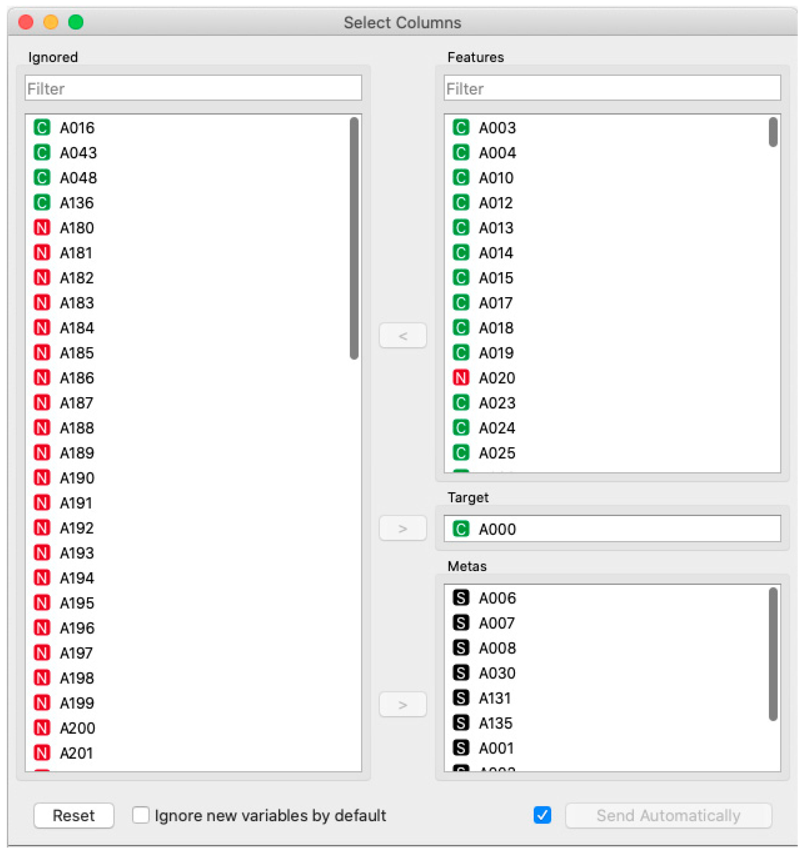
The select column widget was used to identify which attributes were of the metadata type, which ones to use as a class and which ones to use/ignore for the elaboration of the models. In a previous analysis, it was possible to verify that some attributes did not contribute (without data or with the same values for all instances) and, therefore, they were disregarded, as shown in Figure 3. Considering involuntary churn, in which the organization has no interest in keeping the customer due to default issues, the attributes that indicate damage to the operation were also disregarded. After reclassifying the attributes, the configuration was as follows: 77 ignored, 10 meta, and 410 valid attributes.

Selecting a subset of attributes, using its relevance as a criterion, is a way to reduce the dimensionality of the features space, which in this study, due to the large number of variables available for selection, is necessary to reduce the computational and analysis complexity, considering that the increasing number of attributes does not always translate into better result accuracy.

To select the most significant attributes, the rank widget was used, which scores the most relevant variables according to the correlation between them, whether discrete or numerical. Functionality can use algorithms such as:

• Information gain: the expected amount of information (entropy reduction) (Mohammad 2018).
• Gain rate: a ratio between the gain of information and the intrinsic information of the attribute, which reduces the tendency for multivalued resources that occur in the gain of information.
• Gini: the inequality between the values of a frequency distribution.
• ANOVA: the difference between the mean values of the resource in different classes.
• X²: dependency between resource and class measured by chi-square statistics.
• ReliefF: the ability of an attribute to distinguish between classes in similar data instances.
• FCBF (fast correlation based filter): an entropy-based measure, which also identifies redundancies due to peer correlations between resources.

For classification models, a matrix is used where the predicted results are tabulated against the original classes, known as the confusion matrix. This matrix seeks to identify the relationship between successes and errors in the model’s classification.

Table 3. Matrix of confusion.

Confusion Matrix		Predicted by Model
		No Churn	Churn
Real	No Churn	True Negative (TN)	False Positive (FP)
	Churn	False Negative (FN)	True Positive (TP)

shows graphical representation of matrix and confusion. Possible values of the confusion matrix are:

• True positive (true positive–TP) means that the originally predicted and observed class is part of the positive class;
• False positive (false positive–FP) means that the predicted class returned positive, but the original observed was negative;
• True negative (true negative–TN) the predicted and observed values are part of the negative category;
• False negative (false negative–FN) represents that the predicted value resulted in the negative class, but the original observed was of the positive class.

From the confusion matrix, it is possible to assess whether given data was classified correctly or not, against known data, for a given class. Traditionally, the metrics used to validate ranking models are:

• Accuracy: The proportion of correct predictions, without considering what is positive and what is negative;

  $$\mathrm{Accuracy}=\frac{(TP+TN)}{(TP+TN+FP+FN)}$$

  (10)
• Recall (sensitivity): is the proportion of true positives;

  $$\mathrm{Recall}=\frac{(TP)}{(TP+FN)}$$

  (11)
• Specificity: is the proportion of true negatives;

  $$\mathrm{Specificity}=\frac{(TN)}{(TN+FP)}$$

  (12)
• F1: is the harmonic mean between sensitivity and accuracy; that is, it summarizes the information of these two metrics;

  $$\mathrm{F}1==\frac{2}{sesibilidad{e}^{-1}+precisa{o}^{-1}}$$

  (13)
• The ROC curve (receiver operating characteristic) is a metric derived from the confusion matrix, in the sensitivity and specificity dimensions.

To find the best ranking method, the machine learning chosen was the random forest algorithms, as it is less sensitive to data distribution. It was used with the configuration default and the widget test and score to provide the evaluation result. The sampling method chosen was cross-validation with 10 folds and stratified (Yadav and Shukla 2016). For comparison purposes, the metric area under the ROC curve (AUC), F1, accuracy (CA), precision, recall, and specificity were adopted.

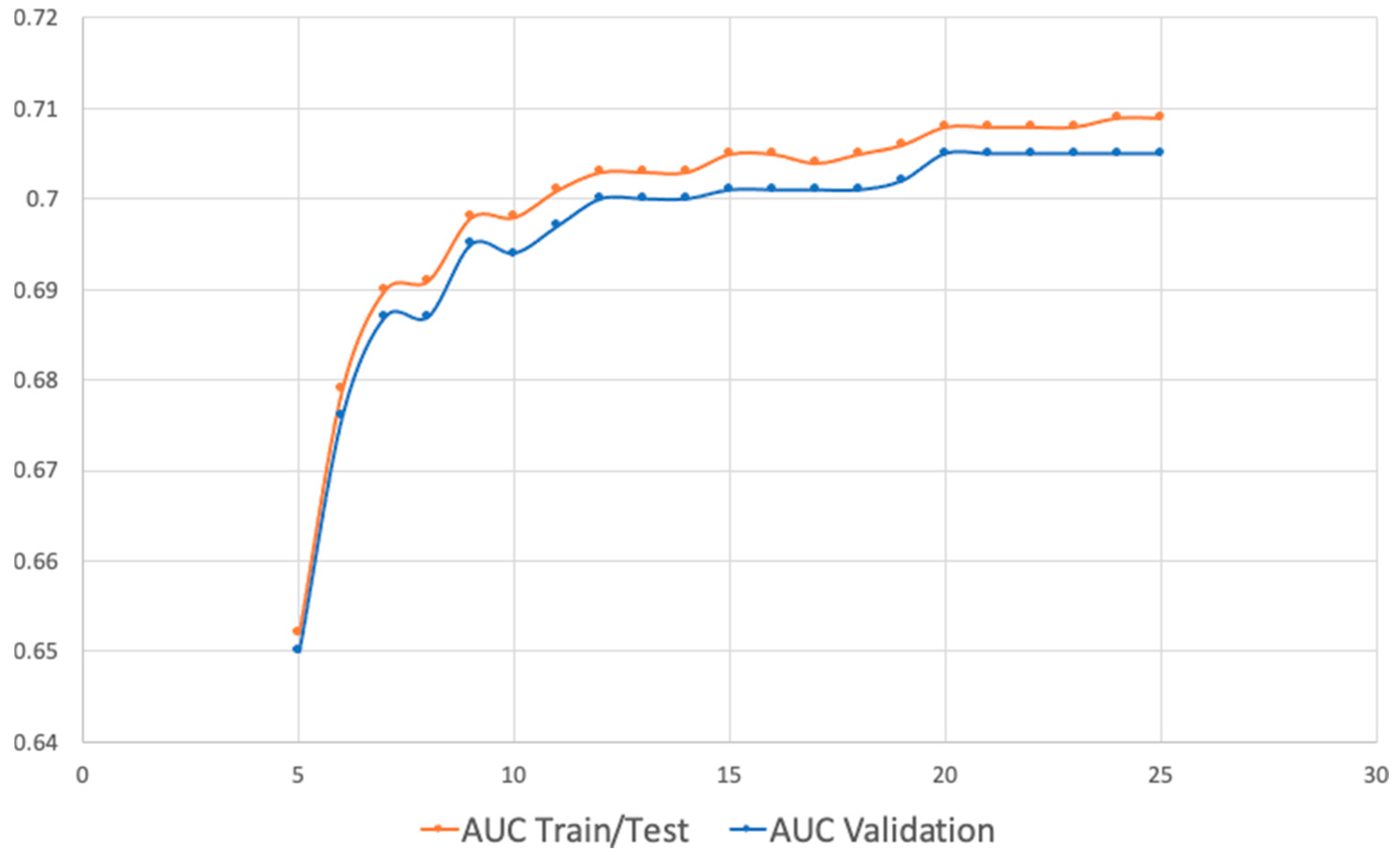
Therefore, the wrapper (forward stepwise selection) technique was adopted, with the construction of a model using random forest, as in the approaches already described, comparing the metrics resulting from the selection of the best n variables. For these selections, the best ranking algorithm (FCBF) was adopted.

Table 4. Selection of attributes with the highest predictive value.

No. Attributes	Training and Testing Metrics
	AUC	Accuracy	F1	Accuracy	Sensitivity	Specificity
5	0.652	0.751	0.696	0.752	0.751	0.427
6	0.679	0.752	0.696	0.755	0.752	0.425
7	0.69	0.755	0.699	0.761	0.755	0.429
8	0.691	0.754	0.698	0.76	0.754	0.428
9	0.698	0.755	0.698	0.765	0.755	0.427
10	0.698	0.755	0.698	0.765	0.755	0.426
11	0.701	0.755	0.699	0.766	0.755	0.427
12	0.703	0.758	0.707	0.761	0.758	0.443
13	0.703	0.757	0.706	0.761	0.757	0.441
14	0.703	0.758	0.707	0.762	0.758	0.443
15	0.705	0.757	0.706	0.762	0.757	0.441
16	0.705	0.757	0.705	0.762	0.757	0.439
17	0.704	0.757	0.704	0.762	0.757	0.438
18	0.705	0.757	0.704	0.762	0.757	0.437
19	0.706	0.757	0.703	0.767	0.757	0.434
20	0.708	0.757	0.703	0.767	0.757	0.434
21	0.708	0.757	0.702	0.768	0.757	0.432
22	0.708	0.757	0.702	0.769	0.757	0.432
23	0.708	0.757	0.702	0.769	0.757	0.432
24	0.709	0.757	0.702	0.769	0.757	0.431
25	0.709	0.757	0.702	0.769	0.757	0.431

and Figure 4 show the results of tests performed with 1 to 25 best ranked attributes. As can be seen, from the 20th variables onwards, the improvements achieved were insignificant, with the greater use of 20 variables proving innocuous.

Regarding the data preparation stage, it is concluded that, for the studied data, the best performing algorithm to filter the most relevant attributes was the FCBF (fast correlation based filter). Through the result obtained through the random forest, without optimization, it was possible to select 20 attributes (from the initial 496), returning classification hits with levels close to 70%.

3.3. Modeling

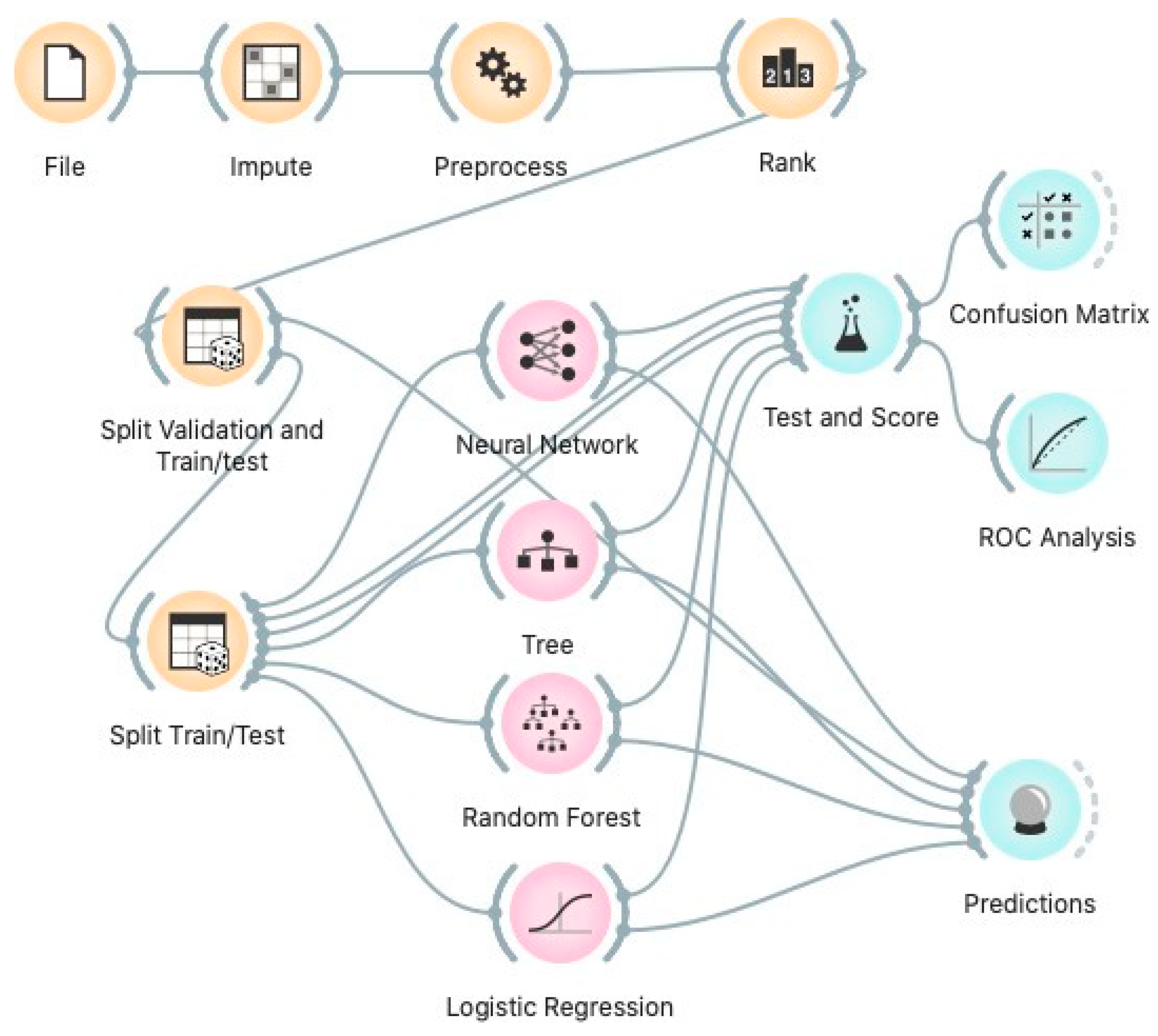
As already mentioned, in Orange the model is represented by means of a flowchart containing the entire structure of the learning process with all the configuration, visualization and operation steps to which the data are submitted, including, but not limited to the application of specific algorithms, visualization of data at a certain stage of the flow, presentations of results and statistics on modifiers applied to the data, segregation of sampling for training and testing, among several other steps inherent to the mining process. Figure 5 illustrates the proposed model contemplating the steps of pre-processing, training, testing and validation.

For model validation purposes, it was decided to divide the data sample into training, testing and validation, in the proportion of 60%, 20%, and 20%, so two data sampler widgets were used. The first separates the data into validation (20% of the data, equivalents to 40,000 instances) and training/test (80% of the data, that is 160,000 instances), and the second for training (75% of the 80% of the data, making a total of 120,000 cases) and testing (25% of the 80% of the data, making a total of 40,000 instances). Training and testing are connected to the test and scores widgets while the validation data (separated in the first data sampler widgets were used to perform the prediction of the models, in order not to use the same values of the instances used to train and test the models, which could result in biased results.

3.3.1. Neural Network

The neural network widget uses the multi-layer perceptron algorithm that can learn nonlinear as well as linear models. The algorithm is based on the skleran library and can be configured as follows:

• Neurons in hidden layers;
• Activation;
• Optimizers;
• Alpha;
• Iterations.

To identify the best configuration of the neural network hyperparameters, the random search method was used, gradually changing each parameter, and collecting the resulting AUC and F1 metrics for each adjusted value. To mitigate the risk of an overfitted model, the model was subjected to 10 different samples, with the same number of instances and in a stratified way, with data not used in training and testing. For each sample, the values of AUC and F1 were obtained and with these values the means (x) and standard deviation (s2) for each configuration were calculated, according to

Table 5. Random search for neural network hyperparameters.

No. Tests	Hyperparameters					Training and Testing						Validation
	(a)	(b)	(c)	(d)	(e)	AUC	Accuracy	F1	Accuracy	Sensitivity	Specificity	AUC x ± s2	F1 x ± s2
1	100	ReLu	Adam	0.0001	200	0.704	0.756	0.710	0.751	0.756	0.453	0.704 ± 0.011	0.711 ± 0.008
2	150	ReLu	Adam	0.0001	200	0.706	0.757	0.714	0.750	0.757	0.461	0.706 ± 0.011	0.713 ± 0.008
3	200	ReLu	Adam	0.0001	200	0.709	0.756	0.714	0.746	0.756	0.463	0.705 ± 0.011	0.718 ± 0.007
4	300	ReLu	Adam	0.0001	200	0.711	0.758	0.719	0.746	0.758	0.474	0.713 ± 0.013	0.717 ± 0.007
5	400	ReLu	Adam	0.0001	200	0.711	0.757	0.720	0.743	0.757	0.479	0.707 ± 0.013	0.715 ± 0.009
6	500	ReLu	Adam	0.0001	200	0.715	0.755	0.722	0.738	0.755	0.488	0.716 ± 0.012	0.723 ± 0.007
7	600	ReLu	Adam	0.0001	200	0.715	0.757	0.721	0.743	0.757	0.482	0.711 ± 0.012	0.72 ± 0.007
8	700	ReLu	Adam	0.0001	200	0.712	0.755	0.721	0.740	0.755	0.485	0.715 ± 0.012	0.722 ± 0.007
9	500	tanh	Adam	0.0001	200	0.710	0.758	0.720	0.748	0.758	0.476	0.711 ± 0.009	0.722 ± 0.006
10	500	Logistic	Adam	0.0001	200	0.713	0.759	0.719	0.750	0.759	0.473	0.711 ± 0.011	0.72 ± 0.007
11	500	Identity	Adam	0.0001	200	0.669	0.732	0.660	0.720	0.732	0.375	0.668 ± 0.016	0.658 ± 0.007
12	500	ReLu	L-BFGS-B	0.0001	200	0.708	0.757	0.718	0.745	0.757	0.472	0.709 ± 0.009	0.719 ± 0.006
13	500	ReLu	SGD	0.0001	200	0.701	0.756	0.708	0.751	0.756	0.448	0.7 ± 0.012	0.705 ± 0.008
14	500	ReLu	Adam	0.0001	100	0.711	0.757	0.717	0.746	0.757	0.470	0.712 ± 0.011	0.713 ± 0.007
15	500	ReLu	Adam	0.0001	50	0.709	0.757	0.713	0.750	0.757	0.460	0.707 ± 0.011	0.711 ± 0.008
16	500	ReLu	Adam	0.0001	300	0.712	0.757	0.719	0.746	0.757	0.475	0.715 ± 0.011	0.719 ± 0.006
17	500	ReLu	Adam	0.0001	400	0.714	0.758	0.720	0.746	0.758	0.476	0.715 ± 0.011	0.719 ± 0.006
18	500	ReLu	Adam	0.01	200	0.708	0.758	0.713	0.752	0.758	0.458	0.706 ± 0.013	0.712 ± 0.009
19	500	ReLu	Adam	1	200	0.692	0.753	0.700	0.751	0.753	0.434	0.689 ± 0.014	0.698 ± 0.009
20	500	ReLu	Adam	50	200	0.522	0.711	0.591	0.506	0.711	0.289	0.623 ± 0.014	0.591 ± 0
21	500	ReLu	Adam	100	200	0.497	0.711	0.591	0.506	0.711	0.289	0.634 ± 0.013	0.591 ± 0
22	500	ReLu	Adam	500	200	0.498	0.711	0.591	0.506	0.711	0.289	0.616 ± 0.012	0.591 ± 0
23	500	ReLu	Adam	1000	200	0.494	0.711	0.591	0.506	0.711	0.289	0.596 ± 0.011	0.591 ± 0

.

Twenty-three sets were tested and the line in bold (6) was the one that obtained the best AUC and F1 value, respecting the mean and standard deviation range.

3.3.2. Decision Tree

The widget tree is an algorithm that divides the data into nodes to find the desired class. It can handle both discrete and continuous datasets and can be used for classification and regression. Here are the tuning settings for algorithm optimization:

• Minimum number of instances in sheets;
• Do not separate subsets;
• Maximum depth limit.

With an approach analogous to that used in neural networks, each hyperparameter of the decision tree was tested and after 20 attempts it was possible to find the ideal configuration for model optimization, without the occurrence of overlapping, according to

Table 6. Random search for decision tree hyperparameters.

No. Tests	Hyperparameters			Training and Testing						Validation
	(a)	(b)	(c)	AUC	F1	Accuracy	Accuracy	Sensitivity	Specificity	AUC x ± s2	F1 X ± s2
1	5	5	3	0.669	0.753	0.700	0.753	0.753	0.432	0.664 ± 0.013	0.695 ± 0.01
2	3	5	3	0.669	0.753	0.700	0.753	0.753	0.432	0.664 ± 0.013	0.695 ± 0.01
3	7	5	3	0.669	0.753	0.700	0.753	0.753	0.432	0.664 ± 0.013	0.695 ± 0.01
4	9	5	3	0.669	0.753	0.700	0.753	0.753	0.432	0.664 ± 0.013	0.695 ± 0.01
5	5	3	3	0.669	0.753	0.700	0.753	0.753	0.432	0.664 ± 0.013	0.695 ± 0.01
6	5	7	3	0.669	0.753	0.700	0.753	0.753	0.432	0.664 ± 0.013	0.695 ± 0.01
7	5	9	3	0.669	0.753	0.700	0.753	0.753	0.432	0.664 ± 0.013	0.695 ± 0.01
8	5	5	5	0.687	0.755	0.704	0.756	0.755	0.440	0.678 ± 0.013	0.706 ± 0.009
9	5	5	7	0.697	0.758	0.711	0.757	0.758	0.451	0.688 ± 0.013	0.706 ± 0.009
10	5	5	9	0.702	0.759	0.715	0.756	0.759	0.459	0.697 ± 0.011	0.71 ± 0.009
11	5	5	11	0.707	0.760	0.720	0.753	0.760	0.472	0.702 ± 0.009	0.717 ± 0.009
12	5	5	13	0.710	0.761	0.726	0.750	0.761	0.487	0.709 ± 0.011	0.726 ± 0.01
13	5	5	15	0.714	0.762	0.731	0.749	0.762	0.503	0.715 ± 0.012	0.731 ± 0.011
14	5	5	20	0.726	0.762	0.743	0.746	0.762	0.548	0.727 ± 0.012	0.742 ± 0.009
15	5	5	25	0.735	0.757	0.747	0.744	0.757	0.584	0.74 ± 0.012	0.749 ± 0.009
16	5	5	30	0.741	0.753	0.748	0.745	0.753	0.610	0.747 ± 0.012	0.752 ± 0.009
17	5	5	35	0.744	0.750	0.748	0.746	0.750	0.622	0.752 ± 0.012	0.752 ± 0.009
18	5	5	40	0.745	0.749	0.748	0.746	0.749	0.629	0.755 ± 0.012	0.753 ± 0.008
19	5	5	50	0.746	0.748	0.747	0.746	0.748	0.631	0.755 ± 0.012	0.754 ± 0.008
20	5	5	55	0.746	0.748	0.747	0.746	0.748	0.632	0.755 ± 0.012	0.754 ± 0.008

. The bold line denotes the best setting, with the AUC and F1 metrics within the mean and standard deviation of the 10 validation samples.

As a result, after optimizing the hyperparameters, the decision tree had 22,623 nodes and 11,312 leaves.

3.3.3. Random Forest

The random forest widget implements a set of decision trees, which in turn is trained with a bootstrap sample set. The final model is based on the majority of votes from the individual trees in the forest. As it is an extension of the decision tree seen in the 3.3.2 items, it can also be used for classification and regression. Here are the tuning settings for algorithm optimizations:

• Number of trees;
• Number of attributes considered in each division;
• Balancing the distribution of classes;
• Individual tree depth limit;
• Do not separate subsets.

The same approach as used in the models previously studied was used to identify the best configuration of the random forest hyperparameters. There were 30 attempts, but only in line 28 (in bold) was the best result of the metrics found within the validation range (mean ± standard deviation), as shown in

Table 7. Random search for random forest hyperparameters.

	Hyperparameters					Training and Testing						Validation
No. Tests	(a)	(b)	(c)	(d)	(e)	AUC	F1	Accuracy	Accuracy	Sensitivity	Specificity	AUC x ± s2	F1 x ± s2
1	10	5	Desl.	3	5	0.687	0.753	0.701	0.750	0.753	0.436	0.684 ± 0.014	0.707 ± 0.034
2	50	5	Desl.	3	5	0.689	0.753	0.701	0.752	0.753	0.435	0.684 ± 0.013	0.697 ± 0.009
3	100	5	Desl.	3	5	0.690	0.753	0.701	0.752	0.753	0.435	0.684 ± 0.013	0.697 ± 0.009
4	200	5	Desl.	3	5	0.690	0.753	0.701	0.752	0.753	0.435	0.685 ± 0.013	0.697 ± 0.009
5	300	5	Desl.	3	5	0.690	0.753	0.701	0.752	0.753	0.435	0.686 ± 0.013	0.697 ± 0.009
6	400	5	Desl.	3	5	0.690	0.753	0.701	0.752	0.753	0.435	0.687 ± 0.013	0.697 ± 0.009
7	500	5	Desl.	3	5	0.690	0.753	0.701	0.752	0.753	0.435	0.689 ± 0.013	0.697 ± 0.009
8	600	5	Desl.	3	5	0.690	0.753	0.701	0.752	0.753	0.435	0.686 ± 0.013	0.697 ± 0.009
9	500	3	Desl.	3	5	0.689	0.753	0.700	0.754	0.753	0.434	0.685 ± 0.013	0.697 ± 0.009
10	500	7	Desl.	3	5	0.688	0.753	0.701	0.752	0.753	0.435	0.685 ± 0.013	0.697 ± 0.009
11	500	9	Desl.	3	5	0.685	0.753	0.701	0.752	0.753	0.435	0.684 ± 0.013	0.697 ± 0.009
12	500	5	Lig	3	5	0.690	0.690	0.693	0.698	0.690	0.580	0.685 ± 0.013	0.689 ± 0.008
13	500	5	Desl.	5	5	0.698	0.755	0.702	0.757	0.755	0.755	0.695 ± 0.014	0.699 ± 0.009
14	500	5	Desl.	7	5	0.708	0.757	0.603	0.767	0.757	0.434	0.705 ± 0.013	0.7 ± 0.009
15	500	5	Desl.	9	5	0.717	0.761	0.709	0.770	0.761	0.440	0.715 ± 0.013	0.706 ± 0.009
16	500	5	Desl.	11	5	0.730	0.765	0.717	0.774	0.765	0.456	0.728 ± 0.012	0.715 ± 0.009
17	500	5	Desl.	13	5	0.745	0.771	0.727	0.780	0.771	0.472	0.743 ± 0.012	0.725 ± 0.008
18	500	5	Desl.	15	5	0.761	0.777	0.737	0.785	0.777	0.489	0.761 ± 0.012	0.738 ± 0.01
19	500	5	Desl.	20	5	0.796	0.794	0.765	0.800	0.794	0.540	0.801 ± 0.011	0.77 ± 0.013
20	500	5	Desl.	25	5	0.817	0.807	0.786	0.808	0.807	0.583	0.824 ± 0.01	0.791 ± 0.008
21	500	5	Desl.	30	5	0.826	0.817	0.801	0.815	0.817	0.618	0.835 ± 0.011	0.808 ± 0.009
22	500	5	Desl.	35	5	0.829	0.823	0.809	0.820	0.823	0.640	0.838 ± 0.011	0.815 ± 0.006
23	500	5	Desl.	40	5	0.830	0.825	0.813	0.821	0.825	0.651	0.839 ± 0.011	0.82 ± 0.006
24	500	5	Desl.	45	5	0.830	0.825	0.814	0.821	0.825	0.654	0.839 ± 0.011	0.82 ± 0.006
25	500	5	Desl.	50	5	0.829	0.825	0.814	0.821	0.825	0.654	0.839 ± 0.011	0.822 ± 0.007
26	500	5	Desl.	40	7	0.826	0.820	0.806	0.818	0.820	0.631	0.836 ± 0.012	0.812 ± 0.006
27	500	5	Desl.	40	3	0.832	0.826	0.816	0.821	0.826	0.664	0.842 ± 0.011	0.824 ± 0.006
28	500	5	Desl.	40	2	0.833	0.826	0.817	0.821	0.826	0.667	0.843 ± 0.011	0.824 ± 0.007
29	500	5	Desl.	40	9	0.823	0.816	0.799	0.815	0.816	0.614	0.832 ± 0.011	0.806 ± 0.006
30	500	5	Desl.	40	11	0.820	0.812	0.793	0.812	0.812	0.600	0.829 ± 0.012	0.801 ± 0.005

.

3.3.4. Logistic Regression

The logistic regression widget implements the model of the same name which is characterized by learning a logistic regression model from the data. It is used for sorting only. Here are the tuning settings for algorithm optimization:

• Regularization;
• Cost;
• Balancing.

As with the other models already seen, the choice of hyperparameters followed the same approach as in the previous models. Twenty tests were performed, but in the seventh configuration the best result was found.

Table 8. Random search for logistic regression hyperparameters.

No. Tests	Hyperparameters			Training and Testing						Validation
	(a)	(b)	(c)	AUC	Accuracy	F1	Accuracy	Sensitivity	Specificity	AUC x ± s2	F1 x ± s2
1	Lasso	0.001	Não	0.665	0.730	0.645	0.738	0.730	0.352	0.663 ± 0.016	0.643 ± 0.007
2	Lasso	0.5	Não	0.671	0.731	0.659	0.718	0.731	0.374	0.668 ± 0.016	0.656 ± 0.007
3	Lasso	1	Não	0.671	0.731	0.659	0.718	0.731	0.374	0.668 ± 0.016	0.656 ± 0.007
4	Lasso	50	Não	0.671	0.731	0.659	0.718	0.731	0.374	0.668 ± 0.016	0.656 ± 0.007
5	Lasso	1000	Não	0.671	0.731	0.659	0.718	0.731	0.374	0.668 ± 0.016	0.656 ± 0.007
6	Lasso	0.001	Sim	0.667	0.631	0.647	0.687	0.631	0.617	0.653 ± 0.042	0.647 ± 0.01
7	Lasso	0.5	Sim	0.671	0.657	0.669	0.691	0.657	0.603	0.669 ± 0.016	0.666 ± 0.009
8	Lasso	1	Sim	0.671	0.657	0.669	0.691	0.657	0.603	0.669 ± 0.016	0.666 ± 0.009
9	Lasso	50	Sim	0.671	0.657	0.669	0.691	0.657	0.603	0.669 ± 0.016	0.666 ± 0.009
10	Lasso	1000	Sim	0.671	0.657	0.669	0.691	0.657	0.603	0.669 ± 0.016	0.666 ± 0.009
11	Ridge	0.001	Não	0.670	0.731	0.656	0.721	0.731	0.369	0.668 ± 0.016	0.652 ± 0.006
12	Ridge	0.5	Não	0.671	0.731	0.659	0.718	0.731	0.374	0.668 ± 0.016	0.656 ± 0.007
13	Ridge	1	Não	0.671	0.731	0.659	0.718	0.731	0.374	0.668 ± 0.016	0.656 ± 0.007
14	Ridge	50	Não	0.671	0.731	0.659	0.718	0.731	0.374	0.668 ± 0.016	0.656 ± 0.007
15	Ridge	1000	Não	0.671	0.731	0.659	0.718	0.731	0.374	0.668 ± 0.016	0.656 ± 0.007
16	Ridge	0.001	Sim	0.671	0.657	0.669	0.691	0.657	0.603	0.669 ± 0.016	0.666 ± 0.009
17	Ridge	0.5	Sim	0.671	0.657	0.669	0.691	0.657	0.603	0.669 ± 0.016	0.666 ± 0.009
18	Ridge	1	Sim	0.671	0.657	0.669	0.691	0.657	0.603	0.669 ± 0.016	0.666 ± 0.009
19	Ridge	50	Sim	0.671	0.657	0.669	0.691	0.657	0.603	0.669 ± 0.016	0.666 ± 0.009
20	Ridge	1000	Sim	0.671	0.657	0.669	0.691	0.657	0.603	0.669 ± 0.016	0.666 ± 0.009

shows the values of the hyperparameters and the metrics found.

4. Results

The way to carry out the comparison between models and to visualize the result for the different classes of the dependent variable is the confusion matrix and the ROC curve. For this purpose, the confusion matrix and ROC analysis widgets were used in the proposed flowcharts, with all study models, respectively.

Table 9. Confusion matrix for predictive models of churn.

Models	Confusion Matrix		Predicted by Model
			Evaded	Active
Neural Network	Real Situation	Evaded	3212	7316
		Active	1585	24,354
Decision Tree		Evaded	5802	4726
		Active	4201	21,738
Random Forest		Evaded	6071	4457
		Active	1671	24,268
Logistic Regression		Evaded	5934	4594
		Active	8010	17,929

and

Table 10. Confusion matrix of proportion by prediction for the predictive models of churn.

Models	Confusion Matrix		Predicted by Model
			Evaded	Active
Neural Network	Real Situation	Evaded	67.0%	23.1%
		Active	33.0%	76.9%
Decision Tree		Evaded	58.0%	17.9%
		Active	42.0%	82.1%
Random Forest		Evaded	78.4%	15.5%
		Active	21.6%	84.5%
Logistic Regression		Evaded	42.6%	20.4%
		Active	47.4%	79.6%

contain the confusion matrix for the trained models and proportion for model prediction, by class. Values in bold represent the number of instances correctly sorted.

Table 11. Classification hits of the predictive models of churn.

	Models
Classification	Neural Network		Decision Tree		Random Forest		Logistic Regression
Correctly	27,566	76%	27,540	76%	30,339	83%	23,863	65%
Incorrectly	8901	24%	8927	24%	6128	17%	12,604	35%

displays instances sorted correctly (true positive and negative) and incorrectly (false positive and negative). Values marked in bold represent the best results obtained in the studied models.

Through

Table 12. Metrics obtained from predictive models of churn.

Models	AUC	F1	Accuracy	Precision	Sensitivity	Specificity	CCM	Training Time	Test Time
Neural Network	0.716	0.756	0.722	0.740	0.756	0.488	0.327	7355.623	5.777
Decision Tree	0.754	0.755	0.753	0.752	0.755	0.634	0.395	223.245	0.057
Random Forest	0.843	0.832	0.823	0.827	0.832	0.680	0.568	128.547	54.449
Logistic Regression	0.669	0.654	0.666	0.689	0.654	0.600	0.238	8.746	0.145

, it is also possible to define the measures of: (1) AUC rate; (2) F1 rate; (3) overall accuracy rate of the model; (4) the accuracy rate of positive values; (5) sensitivity rate, known as the true positive rate; (6) specificity rate, called the true negative rate; (7) Matthews correlation coefficient; and (8) training and testing times of each model measured in seconds. Values in bold express the best values obtained for each metric.

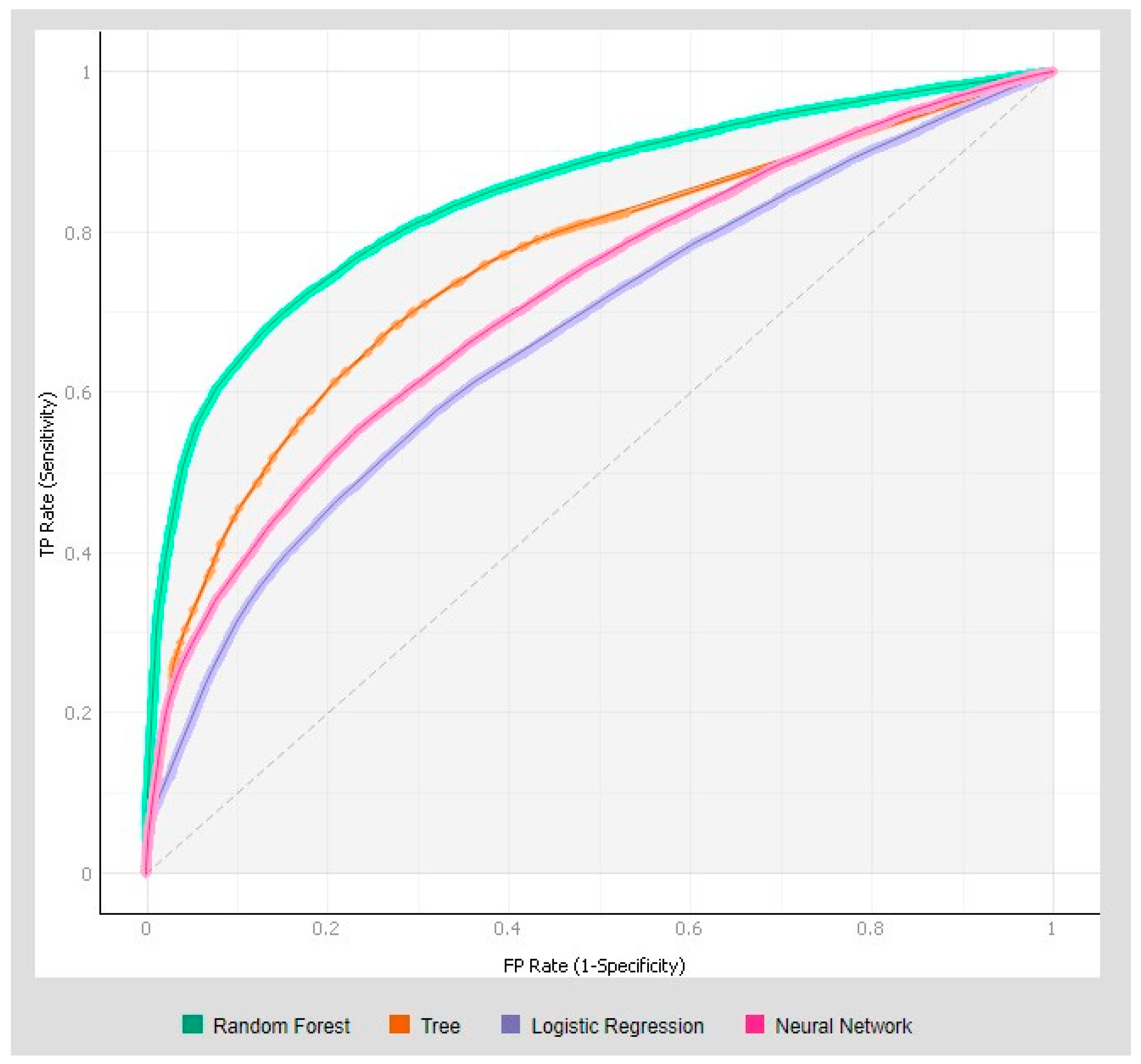
Figure 6 shows the ROC curves of the class ’N’ for each predictive model of churn.

Through a quick observation, it is easily possible to verify the superiority of the random forest model relative to the predictive capacity, which is reflected in all the evaluated metrics. Although it did not excel in any metrics, the decision tree ranked just below the random forest technique. At an intermediate level, with satisfactory results, were the neural network and, lastly, logistic regression.

The ROC curve was obtained by calculating for each cut-off point (represented on the main diagonal) the value of specificity and sensitivity. This curve confirms the good predictive capacity of the model (high sensitivity and specificity), since the more significant the area between the ROC curve and the main diagonal, the better the model’s performances. The model using the random forest technique presented the result of 0.843, which means that there is 84.3% probability that the model correctly classifies each customer, a significant influence when the possible outcomes are dichotomous.

5. Discussion

The main reason for applying analytics and data mining techniques to a corporate churn prevention strategy is to optimize the use of available monetary or personnel resources. With limited funds, in a mass prevention campaign, the amounts to invest on each client are limited. On the other hand, resources can be wasted on customers who are not, in fact, at risk of being lost. The application of data mining techniques allows you to reduce waste and increase the value you invest in your target customers.

Since this work aimed to identify which customers tend to churn, notably, we have sensitivity as the main metric for evaluating the models, as this expresses the amount of positives correctly classified by the model. From this perspective, the model that used the random forest technique reached 83.2%, followed by neural network and decision tree with 75.6% and 75.5%, respectively, and, well below the others, logistic regression with only 65.4%. For the random forest, this means practically saying that the model manages to classify 83 customers out of every 100 customers.

Of the expected customers who will evade, according to Table 10, the random forest model presented the best accuracy, with 78.4% accuracy. If, for example, a preventive retention action is structured aimed at customers expected to evade by the model, 78 out of every 100 selected customers avoided. The other 22 out of 100 were false positives, wrongly considered evaded, who would be covered by the withholding action unnecessarily. Similarly, the model was also able to correctly identify approximately 85 correctly out of every 100 customers that would remain active. Therefore, the higher the accuracy, the lower the level of waste. In the context of a banking organization, business cancellations due to customer abandonment can represent billions of dollars in a year for medium to large banks. Thus, the random forest precision, with low waste, brings operational efficiencies to the banking organization, reducing the loss or loss of revenue.

6. Conclusions

According to the theoretical framework, there is a need for companies to be focused on the customer. For this purpose, it is essential to understand the relationship stages, with methods and processes that enable monitoring and management. To increase profitability or even to remain active in the market, the company must avoid reducing its customer base. Predicting which customers are about to evade, or migrate to a competitor, with the intention of providing mechanisms to avoid this situation is an issue that can be solved through predictive analytics methodologies, allowing for proactive management by organizations. In the context of Brazilian financial institutions, especially in banking organizations, there are few theoretical studies on predictive approaches, which, among other factors, may be characteristic of an incipient culture of predictive approaches to support retention. Consequently, after applying the churn model, it was possible to draw the profile of the customers most likely to drop out, as well as those least likely. Another important factor to consider is that for each customer who fails to evade, there is a reduction in the risk of the customer making negative comments about the company (risk management). In addition, keeping a client is on average five times cheaper than acquiring a new one (financial management).

Through bibliometric analysis of the studies collected in the Web Of Science and SCOPUS indexing bases, it was possible to verify that the most used algorithms in the consulted works dealing with churn predictive models are artificial neural network, decision tree, random forest, and logistic regression algorithms, in that order.

The results obtained show evidence that the proposed models can be efficient in determining the risk of customer abandonment, based on relevant predictive variables. In the base analyzed, of the 497 attributes analyzed, with only 20 was it possible to reach levels close to 70% accuracy in the classification.

Table 11 showed that the overall hit rate of the random forest model is 83% and the ROC curve presented a hit rate of 84.3%. The model was also superior in precision and sensitivity metrics (82.7% and 83.2%), being also ideal in relation to neural network, decision tree and logistic regression.

Although the decision tree model presented a 9% lower predictive capacity in the ROC curve, compared to the random forest model, the former more easily presents and interprets the results, and can be read by people without advanced technical knowledge, providing clarity on which variable should be addressed to mitigate dropout, making it a good option for the organization depending on the level of acceptance of classification accuracies.

It is possible that in more robust databases, which allow overcoming the weighted limitations in relation to the number of customers in the sample and the verified heterogeneity, the performance of all models will probably evolve, notably the random forest and artificial intelligence neural networks algorithms, adherent to the levels of results observed in the academic literature dealing with the subject.

7. Method Limitations

One of the limitations of this study is that the entire database was extracted from a specific operating segment of the banking organization, and the results obtained may not be the same for the other products/segments, which have different dynamics in the life cycle of the credit transaction.

The reduction in turnover is not always due to churn. In many cases, the reduction or cancellation of products results from the loss of interest/need by the customer. There are clients who redeem their investments to invest in the acquisition of a property, for example, others settle credit operations because they no longer need it. At the level of quantitative analysis, with the data collected, we do not see ways to distinguish these occurrences, which is also a limitation of the method.

8. Future Works

In carrying out this work, the predictor variables used were based on the context of the client, behavior, and risk, without evaluating factors external to the bank. However, considering that involuntary churn is due to various factors, such as the customer’s ability to pay or rates that are no longer attractive, it essential to assess whether macroeconomic variables, such as inflation, levels of prices, growth rate, national income, gross domestic product (GDP), and variation in unemployment rates have a significant influence on the dropout rate.

It is also suggested to apply other data mining techniques for the classification tasks with meta classifier algorithms, such as, for example, AdaBoostM1, Bagging and Logit Boost, or the use of a combination of mining algorithms in the classification task using different classifier committee methods, such as stacking and vote, or machine learning with multicriteria. Finally, performing a comparative analysis of the performance of these techniques with the others used in this research could be the focus of another work (Silva et al. 2017).

References

- Adebiyi, Sulaimon Olanrewaju, Emmanuel Olateju Oyatoye, and Bilqis Bolanle Amole. 2016. Improved customer churn and retention decision management using operations research approach. EMAJ Emerging Markets Journal 6: 12–21. [Google Scholar] [CrossRef] [Green Version]
- Buckinx, Wouter, and Dirk Van den Poel. 2005. Customer base analysis: Partial defection of behaviorally loyal clients in a non-contractual FMCG retail setting. European Journal of Operational Research 164: 252–68. [Google Scholar] [CrossRef]
- Burger, Scott V. 2018. Introduction to Machine Learning with R: Rigorous Mathematical Analysis. Sebastopol: O’Reilly Media, Inc. [Google Scholar]
- Camilo, Cássio Oliveira, and João Carlos da Silva. 2009. Mineração de dados: Conceitos, tarefas, métodos e ferramentas. Universidade Federal de Goiás (UFC) 1: 1–29. [Google Scholar]
- Chapman, Pete, Julian Clinton, Randy Kerber, Thomas Khabaza, Thomas Reinartz, Colin Shearer, and Wirth R. 2000. CRISP-DM 1.0: Step-by-Step Data mining Guide. Chicago: SPSS Inc., 76p. [Google Scholar]
- Ciaburro, Giuseppe, and Balaji Venkateswaran. 2017. Neural Networks with R: Smart models using CNN, RNN, Deep Learning, and Artificial Intelligence principles. Birmingham: Packt Publishing Ltd. [Google Scholar]
- Creswell, John W., and J. David Creswell. 2017. Research Design: Qualitative, Quantitative, and Mixed Methods Approaches. Thousand Oaks: Sage Publications. [Google Scholar]
- Demšar, Janez, Tomaž Curk, Aleš Erjavec, Črt Gorup, Tomaž Hočevar, Mitar Milutinovič, Martin Možina, Matija Polajnar, Marko Toplak, Anže Starič, and et al. 2013. Orange: Data mining toolbox in Python. The Journal of Machine Learning Research 14: 2349–53. [Google Scholar]
- Depren, Serpil Kilic. 2018. Churn propensity model for customers who made a complaint in retail banking. European Journal of Business and Social Sciences 6: 48–61. [Google Scholar]
- Flach, Peter. 2012. Machine Learning: The Art and Science of Algorithms that Make Sense of Data. Cambridge: Cambridge University Press. [Google Scholar]
- Ghorbani, Amineh, and Fattaneh Taghiyareh. 2009. CMF: A framework to improve the management of customer churn. Paper presented at 2009 IEEE Asia-Pacific Services Computing Conference (APSCC), Singapore, December 7–11; pp. 457–62. [Google Scholar]
- Harrington, Peter. 2012. Machine Learning in Action. Shelter Island: Manning Publications Co. [Google Scholar]
- He, Benlan, Shi Yong, Wan Qian, and Zhao Xi. 2014. Prediction of customer attrition of commercial banks based on SVM model. Procedia Computer Science 31: 423–30. [Google Scholar] [CrossRef] [Green Version]
- Idris, Adnan, Asifullah Khan, and Yeon Soo Lee. 2012. Genetic programming and adaboosting based churn prediction for telecom. Paper presented at 2012 IEEE International Conference on Systems, Man, and Cybernetics (SMC), Seoul, Korea, October 14–17; pp. 1328–32. [Google Scholar]
- Jahanzeb, Sadia, and Sidrah Jabeen. 2007. Churn management in the telecom industry of Pakistan: A comparative study of Ufone and Telenor. Journal of Database Marketing & Customer Strategy Management 14: 120–29. [Google Scholar]
- Jain, Anil K., Jianchang Mao, and K. Moidin Mohiuddin. 2021. Capítulo 4–O Neurônio, Biológico e Matemático. In Deep Learning Book. Academia: Available online: https://www.deeplearningbook.com.br/o-neuronio-biologico-e-matematico/ (accessed on 15 September 2021).
- James, Gareth, Witten Daniela, Hastie Trevor, and Tibshirani Robert. 2013. An Introduction to Statistical Learning. Berlin: Springer, vol. 112. [Google Scholar]
- Jesson, Jill, Lydia Matheson, and Fiona M. Lacey. 2011. Doing Your Literature Review: Traditional and Systematic Techniques. Thousand Oaks: Sage. [Google Scholar]
- Kelleher, John D., Brian Mac Namee, and Aoife D’arcy. 2020. Fundamentals of Machine Learning for Predictive Data Analytics: Algorithms, Worked Examples, and Case Studies. Cambridge: MIT Press. [Google Scholar]
- Kubat, Miroslav. 2017. An Introduction to Machine Learning. Berlin: Springer. [Google Scholar]
- Mehta, Nick, Dan Steinman, and Lincoln Murphy. 2016. Customer Success: How Innovative Companies Are Reducing Churn and Growing Recurring Revenue. Hoboken: John Wiley & Sons. [Google Scholar]
- Mishra, Abinash, and U. Srinivasulu Reddy. 2017. A comparative study of customer churn prediction in telecom industry using ensemble based classifiers. Paper presented at 2017 International Conference on Inventive Computing and Informatics (ICICI), Coimbatore, India, November 23–24; pp. 721–25. [Google Scholar]
- Mohammad, Adel Hamdan. 2018. Comparing two feature selections methods (information gain and gain ratio) on three different classification algorithms using arabic dataset. Journal of Theoretical & Applied Information Technology 96: 1561–1569. [Google Scholar]
- Montgomery, Douglas C., Elizabeth A. Peck, and G. Geoffrey Vining. 2021. Introduction to Linear Regression Analysis. Hoboken: John Wiley & Sons. [Google Scholar]
- Potdar, Kedar, Taher S. Pardawala, and Chinmay D. Pai. 2017. A comparative study of categorical variable encoding techniques for neural network classifiers. International Journal of Computer Applications 175: 7–9. [Google Scholar] [CrossRef]
- Pritchard, Alan. 1969. Statistical bibliography or bibliometrics. Journal of Documentation 25: 348–49. [Google Scholar]
- Reichheld, Frederick F., and W. Earl Sasser. 1990. Zero defeofions: Quoliiy comes to services. Harvard Business Review 68: 105–11. [Google Scholar] [PubMed]
- Silva, Thuener, Plácido Rogério Pinheiro, and Marcus Poggi. 2017. A more human-like portfolio optimization approach. European Journal of Operational Research 256: 252–60. [Google Scholar] [CrossRef]
- Steiner, Maria Teresinha Arns, Carnieri Celso, Bruno H. Kopittke, and Pedro J. Steiner Neto. 1999. Sistemas especialistas probabilísticos e redesneuraisna análise do créditobancário. Revista de Administraçãoda Universidade de São Paulo (RAUSP) 1: 56–67. [Google Scholar]
- Torgo, Luis. 2016. Data Mining with R: Learning with Case Studies. Boca Raton: CRC Press. [Google Scholar]
- Tranfield, David, David Denyer, and Palminder Smart. 2003. Towards a methodology for developing evidence-informed management knowledge by means of systematic review. British Journal of Management 14: 207–22. [Google Scholar] [CrossRef]
- Van Eck, Nees Jan, and Ludo Waltman. 2010. Software survey: VOSviewer, a computer program for bibliometric mapping. Scientometrics 84: 523–38. [Google Scholar] [CrossRef] [PubMed] [Green Version]
- Van Eck, Nees Jan, and Ludo Waltman. 2014. Visualizing bibliometric networks. In Measuring Scholarly Impact. Berlin: Springer, pp. 285–320. [Google Scholar]
- Vinicius, Anderson. 2017. Capitulo 6—Redes Neurais Artificiais–Perceptron. In Deep Learning Book. San Francisco: Academia. [Google Scholar]
- Yadav, Sanjay, and Sanyam Shukla. 2016. Analysis of k-fold cross-validation over hold-out validation on colossal datasets for quality classification. Paper presented at 2016 IEEE 6th International Conference on Advanced Computing (IACC), Bhimavaram, India, February 27–28; pp. 78–83. [Google Scholar]
- Yanfang, Qiu, and Li Chen. 2017. Research on E-commerce user churn prediction based on logistic regression. Paper presented at 2017 IEEE 2nd Information Technology, Networking, Electronic and Automation Control Conference (ITNEC), Chengdu, China, December 15–17; pp. 87–91. [Google Scholar]
- Yang, Jing, Changxiu Cheng, Shi Shen, and Shanli Yang. 2017. Comparison of complex network analysis software: Citespace, SCI 2 and Gephi. Paper presented at 2017 IEEE 2nd International Conference on Big Data Analysis (ICBDA), Beijing, China, 10–12 March; pp. 169–72. [Google Scholar]
- Zhu, Bing, Bart Baesens, and Seppe K. L. M. van den Broucke. 2017. An empirical comparison of techniques for the class imbalance problem in churn prediction. Information Sciences 408: 84–99. [Google Scholar] [CrossRef] [Green Version]
Figure 1.
Literature review diagram.
Figure 2.
Network map of terms used in the literature review.
Figure 3.
Selection of relevant attributes for modeling.
Figure 4.
Test chart for choosing the most relevant attributes.
Figure 5.
Suggested model.
Figure 6.
ROC curve of churn predictive models for the escaped class.