
Stress Spillovers among Financial Markets: Evidence from Spain


1
Department of Quantitative Methods for Economics and Management, Faculty of Economics, Universidad de Las Palmas de Gran Canaria, Campus de Tafira, 35001 Las Palmas de Gran Canaria, Spain
2
Auckland Centre for Financial Research, Auckland University of Technology, Auckland 1010, New Zealand
3
Department of Economic Analysis, Faculty of Economics and Business, Universidad Complutense de Madrid, Campus of Somosaguas, 28040 Madrid, Spain
*
Author to whom correspondence should be addressed.
J. Risk Financial Manag. 2021, 14(11), 527; https://0-doi-org.brum.beds.ac.uk/10.3390/jrfm14110527
Submission received: 29 September 2021
/
Revised: 22 October 2021
/
Accepted: 1 November 2021
/
Published: 5 November 2021
(This article belongs to the Special Issue Financial Markets—The Response in Crisis Moments)
Abstract
:Using a unique database, this paper examines the interconnection among stress indicators of the Spanish financial markets during the period of January 1999 to April 2021, applying both the connectedness framework and the Time-Varying Parameter Vector Autoregressive connectedness approach. Our results suggest that 15.67% of the total variance of forecast errors was explained by shocks across the six financial market stress indices examined, indicating that the remaining 84.33% of variation was due to idiosyncratic shocks. Nevertheless, we find that stress connectedness varies over time, with a surge during periods of increasing economic and financial instability, mainly driven by high levels of pandemic and economy policy uncertainty and real economy worsening. Financial intermediaries were the main generators of stress during three out of four recent major financial crises in Spain, while their role as stress transmitters to other markets has been reduced since the onset of the COVID-19 health crisis. Our results also indicate that the COVID-19 outbreak represents a relevant event in the transmission of stress among all market segments.
1. Introduction
In the time since the global financial crisis (GFC), a paramount goal has been to understand how financial vulnerabilities can be transmitted and amplified between markets, and this interest has been reinvigorated by the COVID-19 pandemic.
One important stream of research has focused on quantifying and monitoring the degree of stress transmission in financial markets, and various aggregated financial stress indicators have been proposed in the literature. Among these, the Financial Stress Indices (FSIs) have played a key role in capturing the level of financial stress in real time. The seminal paper by Illing and Liu (2006) developed an FSI for the Canadian financial system and proposed several approaches to aggregate individual stress indicators into a composite stress index.1 In the same vein, Holló et al. (2012) introduced a Composite Indicator of Systemic Stress (CISS) for the Euro Area (EA) based on data on five segments (equity markets, bond markets, money markets, financial intermediaries, and forex markets) of European financial markets that are available monthly.
In this paper, we use stress indicators for six financial market segments of the Spanish Financial Market Stress Indicator (FMSI), a coincident measure of systemic risk developed by the National Securities Market Commission (CNMV, the Spanish government agency responsible for the financial regulation of the securities markets in Spain) to quantify the transmission of stress in the Spanish financial system. This indicator is similar to a CISS and has the advantage of being updated weekly, allowing a real-time evaluation of financial stress. Moreover, it offers disaggregated market-based financial stress measures for five categories.
With this goal in mind, we make two major contributions to the extant literature. First, we analyse connectedness between segments using a framework proposed by Diebold and Yilmaz (2014), providing insights on the comparison of the extent and nature of interdependencies (and spillovers between them) that could allow portfolio investors and macroprudential regulators to design more effective asset allocation, portfolio rebalancing, and risk management strategies. Second, we implement the Time-Varying Parameter Vector Autoregressive (TVP-VAR) connectedness approach developed by Antonakakis et al. (2018) to evaluate both the net directional connectedness for each segment (to identify episodes of financial stress intensification) and the role played by each segment in propagating systemic risk during recent crisis shocks.2
We consider this to be an interesting case study, as Spain was heavily affected by the GFC of 2007–2008 and by the subsequent European sovereign debt crisis of 2010–2012, and because Spain is among the EA countries worst affected by COVID-19 pandemic, with profound economic impacts. Therefore, our analysis can help in assessment of the workings of specific transmission channels of financial spillover and contagion risks in the EA.
The main findings are summarised as follows. In the first step, we find a system-wide value of 15.67% for the total connectedness between the six stress indices under study for the full sample period, indicating that the remaining 84.33% of variation was due to idiosyncratic shocks. In the second step, we analyse the dynamic nature of the total connectedness, obtaining evidence of strong spillovers between market segments with a large variation over time. This finding supports the literature showing that stress transmission across market segments increases during times of financial turbulence. After evaluating total directional connectedness, we use regression techniques to analyse their determinants, finding that it is mainly driven by high levels of pandemic and economic policy uncertainty and real economy deterioration. In a third step, we examine the time-varying net spillovers across stress indices. Across all the major financial crises in the recent history of the Spanish economy, we identify the financial intermediaries segment (which mostly represents the banking sector) as the major generator of stress to the Spanish financial system, although the equity and bond markets triggered stress to the system during the COVID-19 pandemic. This suggests a healthier position of the Spanish financial intermediaries during the COVID-19 crisis period, with a gradual reduction in their role as stress transmitters to other market segments as compared to prior crises. Our results also indicate a significant stress transfer among all market segments during the outbreak, vividly illustrating the impacts of an unanticipated pandemic event that created great uncertainty around the potential duration and intensity of disruption.
The paper proceeds as follows. Section 2 outlines the econometric framework to quantify both the total and directional stress connectedness. Section 3 describes our data and presents a preliminary analysis. In Section 4, we report the empirical results (both static and dynamic) obtained for our sample of stress indicators representative of six relevant market segments (a system-wide measure of connectedness), in addition to exploring the determinants of the dynamic total connectedness and performing a robustness exercise by examining the stress indices for the peripheral European economies. Section 5 examines the evolution of net directional and net pairwise directional connectedness in each market. Finally, Section 6 offers some concluding remarks.
2. Econometric Methodology
This section presents the econometric methodology used in the empirical analysis of the total and directional connectedness between the financial market stress indices analysed in the paper. First, we briefly describe the methodological econometric framework of Diebold and Yilmaz (2014). Second, we outline the dynamic connectedness procedure based on the TVP-VAR provided by Antonakakis et al. (2018).
2.1. Diebold and Yilmaz’s Connectedness
Given a multivariate empirical time series, the forecast error variance decomposition is obtained from the following steps:
- Fit a reduced-form vector autoregressive (VAR) model to the series:where represents an N × 1 series vector at time t, is an N × Np dimensional coefficient matrix, and is an N × 1 dimensional error disturbance vector with an N × N variance–covariance matrix,
- Using series data up to and including time t, establish an H period-ahead forecast (up to time t + H).
- Decompose the error variance of the forecast for each component with respect to shocks from the same or other components at time t.
Diebold and Yilmaz (2014) propose several connectedness measures built from pieces of variance decomposition, in which the forecast error variance of variable i is decomposed into parts attributed to the various variables in the system. Their approach has the considerable advantage of fully accounting for contemporaneous effects, and it also directly measures not only the direction but the strength of linkages among the variables under study. This subsection provides a summary of their connectedness index methodology.
Let us denote by the ij-th H-step variance decomposition component (i.e., the fraction of variable i’s H-step forecast error variance due to shocks in variable j). The connectedness measures are based on the “non-own” or “cross” variance decompositions,
Consider an N-dimensional covariance stationary data-generating process (DGP) with orthogonal shocks: Note that need not be diagonal. All aspects of connectedness are contained in this very general representation. Contemporaneous aspects of connectedness are summarised in and dynamic aspects in . The transformation of via variance decompositions is needed to reveal and compactly summarise connectedness. Diebold and Yilmaz (2014) propose a connectedness table such as Table 1 to understand the various connectedness measures and their relationships. The main upper-left N × N block, which contains the variance decompositions, is called the “connectedness matrix” and is denoted by
The connectedness table increases , with the rightmost column containing row sums, the bottom row containing column sums, and the bottom-right element containing the grand average in all cases for
The off-diagonal entries of are the parts of the N forecast error variance decompositions of relevance from a connectedness perspective. In particular, the gross pairwise directional connectedness from j to i is defined as follows:
Since in general the net pairwise directional connectedness from j to i can be defined as:
As for the off-diagonal row sums in Table 1, these give the share of the H-step forecast error variance of variable coming from shocks arising in other variables (all others, as opposed to a single other). The off-diagonal column sums provide the share of the H-step forecast error variance of variable going to shocks arising in other variables. Hence, the off-diagonal row and column sums, labelled “from” and “to” in the connectedness table, offer the total directional connectedness measures. In particular, total directional connectedness from others to i is defined as:
and total directional connectedness from j to others is defined as:
We can also define net total directional connectedness as:
Finally, the grand total of the off-diagonal entries in DH (equivalently, the sum of the “from” column or “to” row) measures total connectedness:
For the case of non-orthogonal shocks, the variance decompositions are not as easily calculated as before, because the variance of a weighted sum is not an appropriate sum of variances. Otherwise, methodologies for providing orthogonal innovations such as traditional Cholesky factor identification may be sensitive to ordering. Therefore, following Diebold and Yilmaz (2014), a generalised variance decomposition (GVD), which is invariant to ordering, proposed by Koop et al. (1996) and Pesaran and Shin (1998) will be used. The H-step generalised variance decomposition matrix is defined as , where:
In this case, is a vector with j-th element unity and zeros elsewhere; is the coefficient matrix in the infinite moving-average representation from VAR; is the covariance matrix of the shock vector in the non-orthogonalised-VAR, with being its j-th diagonal element. In this GVD framework, the lack of orthogonality means that the rows of do not have sum unity, and in order to obtain a generalised connectedness index , the following normalisation is necessary, , where by construction and
The matrix permits us to define similar concepts as defined before for the orthogonal case; that is, total directional connectedness, net total directional connectedness, and total connectedness.
Therefore, the use of the Diebold and Yilmaz (2014) framework allows us to measure the future expected variation in i-th financial market stress accounted for by a standard deviation shock to j-th financial market stress, based on variance decompositions where the estimated network structure between the analysed components is complete and links are weighted and directed, making it possible to assess the variables’ comparative importance for others in the network. Furthermore, since the linkages are not bilaterally equal, this methodology captures the asymmetry in connectedness among the financial market segments under study. Additionally, as Arsov et al. (2013) pointed out, Diebold and Yilmaz’s connectedness is highly adaptive to data changes, with its predictive power being one of the highest among other indicators.
2.2. Dynamic Connectedness Based on TVP-VAR
Antonakakis et al. (2018) extended and refined the current dynamic connectedness literature by applying TVP-VAR as an alternative to the currently proposed rolling window VAR. This approach improves the methodology provided by Diebold and Yilmaz (2014) substantially, because under their proposed methodology: (1) there is no need to arbitrarily set the rolling window size; (2) it employs the entire sample to estimate the dynamic connectedness, so there is no major loss of observations; (3) it is not outlier-sensitive. Another advantage of their proposed TVP-VAR-based measure of connectedness is that it adjusts immediately to events (see for example Antonakakis et al. 2018 and Gabauer and Gupta 2018), being able to accommodate both stochastic coefficients and volatilities of the VAR model (Cogley and Sargent 2005). This is essential for our purpose because the relative roles of the stress indicators can change over time. Finally, linear models with TVP are general approximations of arbitrary non-linear models, as emphasised by Granger (2008).
The TVP-VAR methodology allows both the VAR parameters and the covariances to vary via a heteroscedastic volatility Kalman filter estimation with forgetting factors introduced by Koop and Korobilis (2014). As such, this approach can also be conducted to examine dynamic connectedness with limited time series data.
The TVP-VAR model can be written as follows:
where is an N × Np dimensional time-varying coefficient matrix and is an N × 1 dimensional error disturbance vector with an N × N time-varying variance–covariance matrix, , and is the given information through time t − 1. The parameters follow a random path and depend on their own lagged values and on an N × Np dimensional matrix with an Np × Np variance–covariance matrix, .3
The time-varying coefficients and can be used in Diebold and Yilmaz’s connectedness measure, where the dynamic H-step generalised forecast error variance decomposition matrix is now:
which after normalisation would be . Similarly, the matrix permits us to define the dynamic total directional connectedness, net total directional connectedness, and total connectedness.
3. Data and Preliminary Analysis
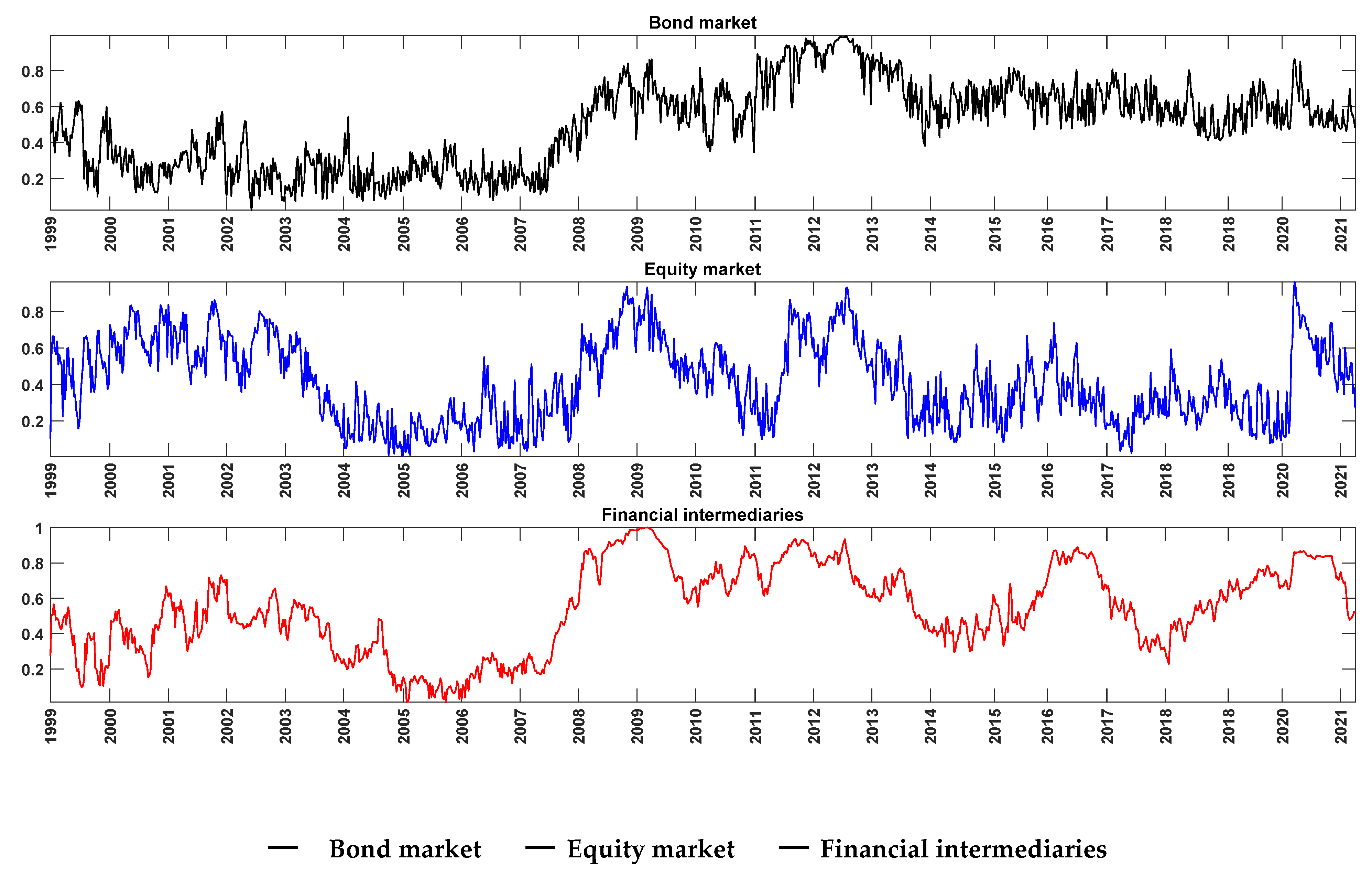
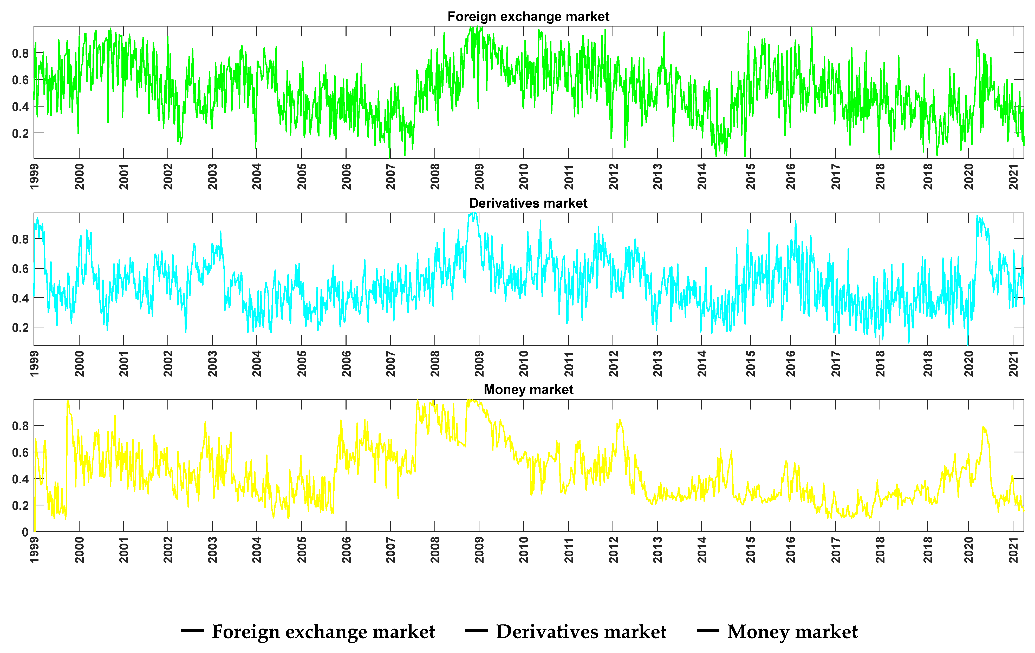
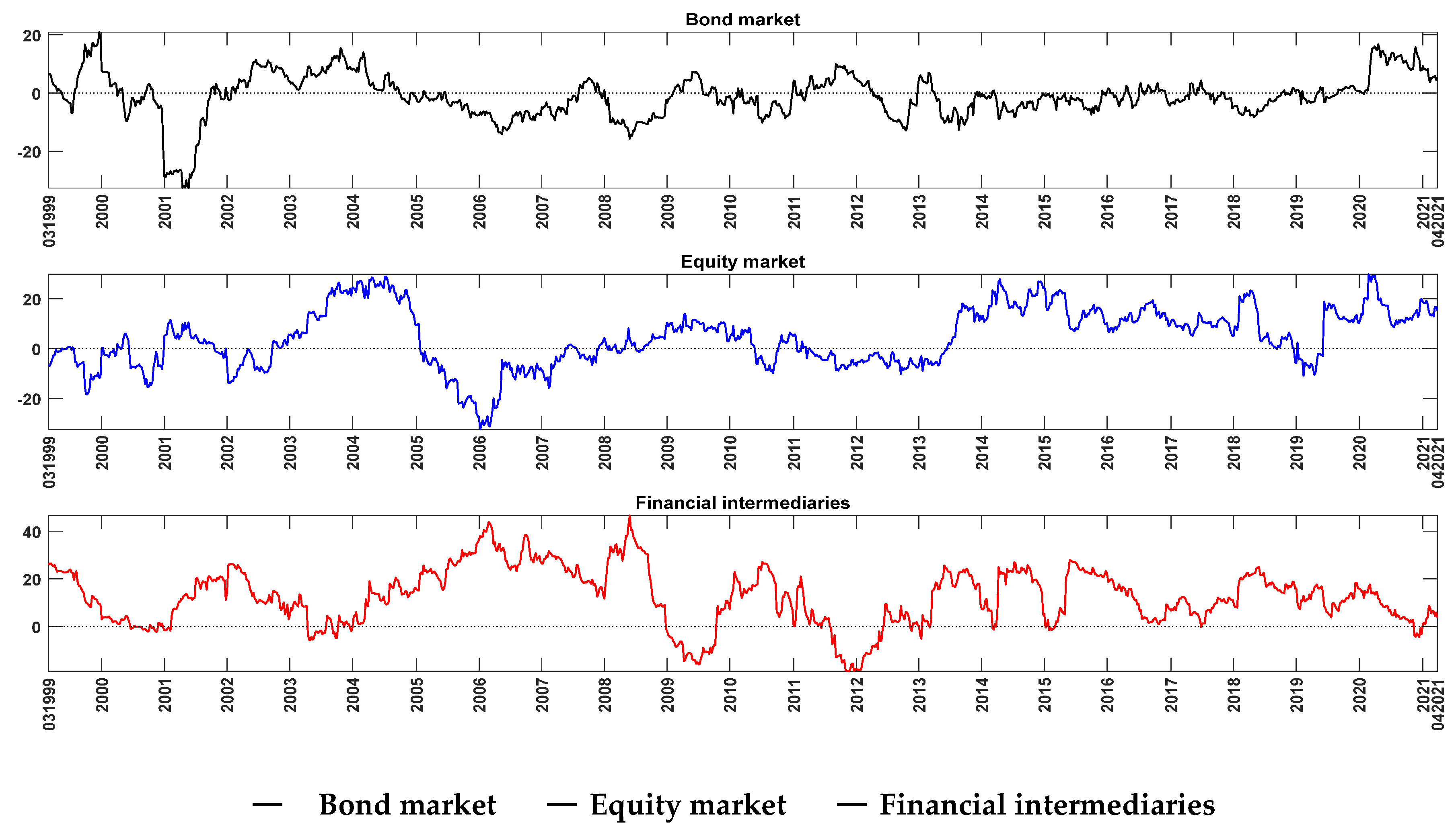
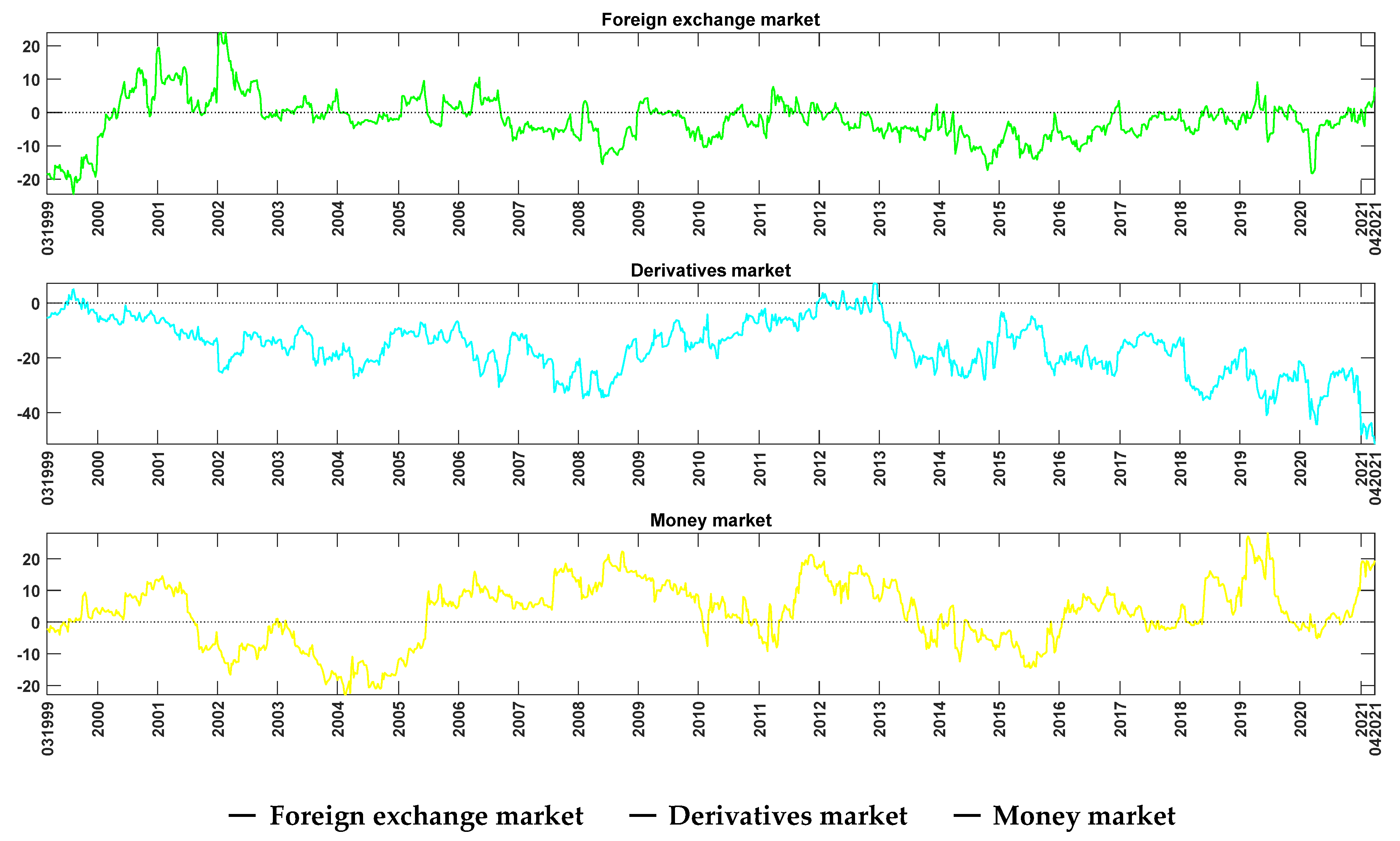
In this paper, a unique database is exploited. It consists of stress indicators for six Spanish financial market segments: the bond market, the equity market, the money market, the financial intermediaries, the foreign exchange market, and the derivatives market.
The bond market stress indicator is related to sovereign risk and takes into account both solvency and liquidity conditions in the corporate bond market and the risk aversion of investors.
The equity markets stress indicator concerns shifts in volatility, liquidity, and sudden asset price movements that are common in periods of financial stress.
The money market stress indicator is intended to reflect liquidity and counterparty risk in the inter-bank market.
The financial intermediaries stress indicator captures their major role in the correct functioning of the financial system and their potential impact on the real economy. This stress indicator mostly represents the banking sector, in addition to a few insurance companies, mutual funds, and investment services firms.
The foreign exchange market stress indicator is considered to reflect large movements in foreign exchange markets, which is particularly relevant not only for those institutions heavily dependent on non-domestic liabilities but also for those with high exposure to non-domestic assets.
Finally, the derivatives market stress indicator represents a special segment of the financial system, as these are based upon the underlying markets.
These indicators are provided weekly by the CNMV and are based on the information received from relevant financial intermediaries, comprising 18 market-based financial stress variables representing changes in volatility, credit spreads, liquidity, and loss of value in different instruments. To the best of our knowledge, no such detailed datasets are available for other European countries to date. As mentioned before, the CNMV also provides the FMSI as a global measure of systemic risk in the Spanish financial system. The stress indicator indices range from 0 (tranquil or low stress period) to 1 (turbulent or high stress period). Our sample spans from 1 January 1999 to 2 April 2021 (i.e., a total of 1162 weekly observations), and it includes several remarkable episodes of the Spanish economy, which we enumerate below.
Panel A of Table 2 presents the descriptive statistics for the series, along with the Jarque–Bera test for normality. The mean ranks between 0.4170 (equity market) and 0.5416 (financial intermediaries). The estimated skewness is negative for financial intermediaries (suggesting that the distribution has a long-left tail), while it is positive for the remaining market segments (indicating that the distribution has a long-right tail). The excess kurtosis is negative in all cases, suggesting that the distribution of the series is flat relative to normal. This asymmetry and platykurtic excess are in line with the Jarque–Bera test results, justifying the rejection of the hypothesis of normal distribution at the 1% significance level. We report the pairwise correlations in panel B of Table 2. All pairwise correlations are positive and highly significant, except for the negative and insignificant correlation between the stress indicators of the bond market and money market segments, suggesting a certain degree of co-movement between these stress indicators of different market segments.
Finally, Figure 1 shows the weekly evolution in the stress indicator of the Spanish financial markets. One can observe several episodes of increased stress that coincide with important events, such as:
- (i.)
- The introduction of euro changeover in the first months of 2002;
- (ii.)
- The GFC of 2007–2008;
- (iii.)
- The EA sovereign debt crisis and signing of the EA fiscal compact in March 2012;
- (iv.)
- The global financial turmoil after the UK voted to leave the European Union (a.k.a. Brexit) in June 2016;
- (v.)
- The outbreak of the COVID-19 pandemic in 2020, requiring many countries to introduce measures restricting activity and movements.
These sample period events have influenced either or both the direction and intensity of dependence across the market segments currently under examination, and they will be the subject of special attention in the empirical sections.
4. Empirical Results
In this section, we report the empirical results of the stress connectedness. First, we examine the static or full-sample GVD table. Second, we analyse the dynamic connectedness through TVP-VAR.
4.1. Static (Full-Sample, Unconditional) Analysis
Table 3 displays the full-sample connectedness, whereby the off-diagonal elements measure the connectedness between the different Spanish financial market stress indicators. As mentioned before, the ij-th entry of the upper-left 6 × 6 market submatrix gives the estimated ij-th pairwise directional connectedness contribution to the forecast error variance of market i’s financial stress coming from innovations to market j. Hence, the off-diagonal column sums (labelled “TO”) and row sums (labelled “FROM”) give the total directional connectedness to all others “from” i and “to” i, respectively. The bottommost row (labelled “net”) gives the difference in the total directional connectedness (to minus from). Finally, the bottom-right element (in boldface) is the total connectedness, which is calculated as the sum of the non-diagonal elements of the connectedness matrix, divided by the number of market segments.4
As can be seen, the diagonal elements (own connectedness) are the largest individual elements in the table, ranging from 69.46% (derivatives market) to 94.94% (money market). Interestingly, the own connectedness is greater than any total directional connectedness from and to others, reflecting that these stress indicators are somewhat independent of each other. Namely, news shocks that affect the stress indicator of a particular market segment spread modestly to the stress indicators of the other market segments. Accordingly, the total connectedness of financial market stress is merely 15.67%, suggesting a low level of interrelatedness across the stress indicators of the six market segments under consideration and indicating that 84.33% of the variation is due to idiosyncratic shocks. This result largely contrasts with both the value of 78.3% obtained by Diebold and Yilmaz (2014) for the total connectedness between U.S. financial institutions and the value of 97.2% found by Diebold and Yilmaz (2012) for international financial markets.
Regarding the net (to minus from) contribution, our results suggest that the derivatives markets are a strong net receiver of financial stress (−22.31%), while the equity market, the financial intermediaries, and the money market are net financial stress triggers (6.11%, 8.62% and 6.43%, respectively). The bond markets and the foreign exchange markets are neither net receivers nor triggers of financial stress, with negligible net contributions of 1.16% and −0.01%, respectively. Finally, the highest observed gross pairwise directional connectedness is from the equity market to the derivatives market (13.21%), followed by that from financial intermediaries to the equity market (9.61%).
In sum, there is a low average static connectedness between the six stress indicators of the Spanish economy. The stress indicator of derivative markets is the largest net receiver of stress from the other indicators, although the equity market, the financial intermediaries, and the money market stress indicators are the major triggers of stress across segments.
4.2. Dynamic Total Connectedness Analysis
The previous subsection provides a snapshot of the “unconditional” or full-sample aspects of the connectedness measures among the financial market stress indices. However, the dynamics of the connectedness measures remain concealed. The appeal of the connectedness methodology lies in its use as a measure of how quickly stress shocks spread across holding periods, as well as within market segments. As previously stated, we carry out an analysis of dynamic connectedness based on TVP-VAR.
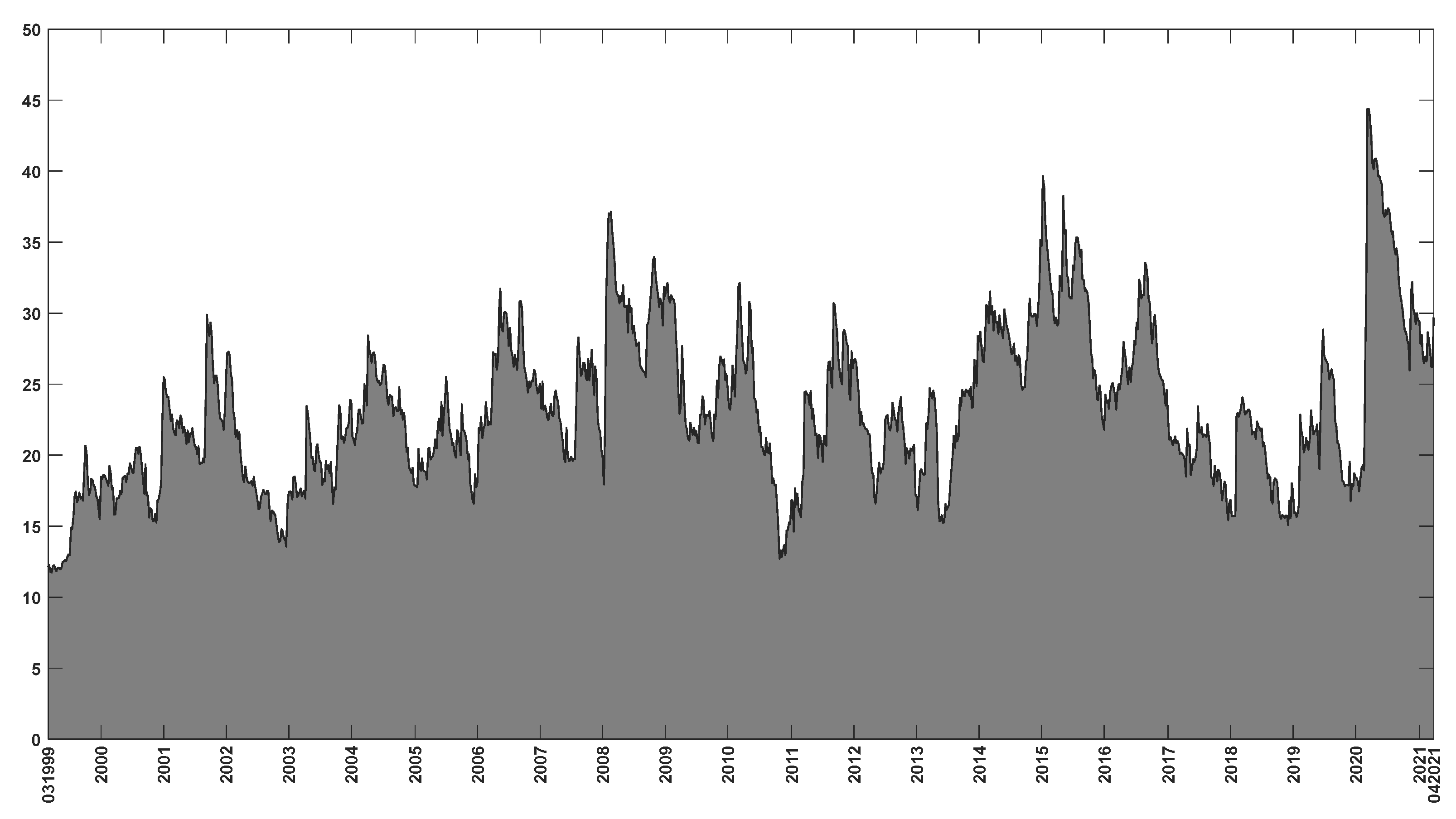
Figure 2 plots the dynamics over time of the total connectedness between the six financial market stress indicators. As expected, total connectedness shows a time-varying pattern over the sample period, ranging from 11.74% to 44.37% and highlighting several cycles of connectedness where the total connectedness is higher or lower than the static full-sample total connectedness of 15.67%. The most remarkable spikes in the total connectedness of the Spanish stress indicators are observed: (i) after the terrorist attacks in the United States on 11 September 2001, which constituted a major shock to the world economy and risked the disruption of financial markets worldwide; (ii) following the March 2004 terrorist attack by Al Qaeda in Madrid, which coincided with national elections in Spain and triggered high uncertainty and stress in the financial markets; (iii) during the international stock market turmoil that began in May 2006 in the context of a global repricing of risk; (iv) during the intensification in 2008 of the financial market turbulences; (v) after the significant deteriorations in several financial market segments in August 2011 due to the spread of EA government bond market tensions; (vi) in the middle of 2015, reflecting market tensions generated by the decision of Greek authorities to hold a referendum and by the non-prolongation of Greece’s second macroeconomic adjustment programme, which generated high stress and uncertainty in the EA; (vii) in 2016, due to the political uncertainty that followed the outcomes of the UK referendum on European Union membership and the U.S. presidential election; (viii) with the onset of coronavirus-related financial market turmoil (March 2020). It is interesting to note that in this last episode, total connectedness between the stress indicators of the different market segments experienced the highest increase, reflecting the unprecedented economic impact of COVID-19, which affected Spain with particular virulence.
Therefore, the full-sample total connectedness of 15.67% reported above undervalues the potential connectedness of the financial market stress indices. These indices seem to be more connected in periods of high market tensions with potential effects across all market segments, making them most vulnerable to contagion.
4.3. Determinants of the Dynamic Total Connectedness
In the previous subsection, we showed that although the full-sample total connectedness is small, there are periods of sizable total connectedness between the the financial market stress indices of Spain. Specifically, these indices seem to be more connected in periods of high market turbulence. In this subsection, we carry out a more formal analysis to identify the potential determinants of the dynamic total stress connectedness measure.5
We consider a set of potential variables that can explain the dynamic total stress connectedness measure. First, we appraise the role of the uncertainty as a key determinant of the total stress connectedness. In particular, we employ two economic uncertainty variables: the World Uncertainty Index (WUI Global) and the Spanish component of the WUI (WUI-Spain). These variables track uncertainty across the globe and within Spain by text mining the country reports of the Economist Intelligence Unit.6 Figure 2 shows how the historical maximum total stress connectedness coincides with the COVID-19 pandemic crisis period. Therefore, we also control for the effect of uncertainty generated by pandemics using Spain’s component of the World Pandemic Uncertainty Index (WPUI-Spain).7 Finally, we take into consideration the economic policy uncertainty of Spain (EPU-Spain) to control for the policy-related economic uncertainty.8
Second, the reaction of the stress indices may also be related to the real economy developments. To assess the role of these developments, we use the Spanish Industrial Production Index (IPI) and GDP (chain-linked volume indices), both corrected by seasonal and calendar effects, from the Spanish National Statistics Institute. Finally, as a measure of the monetary policy page, we use the Shadow Short Rates (SSR) estimates for the euro area based on the research by Krippner (2013) and downloaded from the Reserve Bank of New Zealand website.9 Shadow Short Rate (SSR) estimates are generated regressors proposed as a proxy for policy interest rates during unconventional monetary policy periods in EA. We expect this variable to capture the adoption of easier monetary policies by the ECB during the COVID-19 crisis.
To match the different frequencies of the series, we convert them into the same monthly frequency. Those series with monthly frequency data are unchanged (i.e., EPU-Spain, IPI, and SSR). The weekly dynamic total stress connectedness measure is averaged within the month to obtain the monthly series. We interpolate the quarterly series via a cubic spline to obtain their monthly values (i.e., WUI Global, WUI-Spain, WPUI-Spain and GDP).10 Finally, we apply differences (represented by Δ) in the non-stationary series. 11
We run the following regression by OLS:
where is the total stress connectedness at month t, represents the uncertainty indicators (WUI Global, WUI-Spain, WPUI-Spain and ΔEPU-Spain), represents the economic indicators (ΔIPI, ΔGDP and ΔSSR), and represents the residuals. To facilitate the interpretation, we have standardised all the series. The results are reported in Table 4.
The dynamic total stress connectedness is very persistent with its first positive lag and highly significant at the 1% level. Regarding the uncertainty indicators, model (1) shows that both Spain’s component of the World Pandemic Uncertainty index and Spain’s EPU are positive and significant at the 5% and 10% levels, respectively. Therefore, increases in the pandemic and economic policy uncertainty in Spain are associated with an increase in the total stress connectedness of the Spanish financial system. This result suggests that an important component of the stress in the Spanish economy is the uncertainty regarding economic policies. This finding is in line with both the theoretical framework laid out by Gomes et al. (2012) and Pástor and Veronesi (2012, 2013) on how uncertainty in governmental policies may influence return and volatility dynamics in financial markets and with the numerous subsequent studies providing ample evidence of a policy uncertainty effect on stock and bond markets (see Wisniewski and Lambe 2015; Li et al. 2016; Mei et al. 2018, and Chen and Chiang 2020, among others). Likewise, the pandemic uncertainty, mainly that associated with the COVID-19 pandemic crisis, also represents a key factor of the dynamics in the stress indices. This result could be showing that COVID-19 not only had a severe impact on the global economy and financial markets, but also that the uncertainty regarding the unprecedented government interventions could increase financial market volatility, leading to both abrupt portfolio reconstructions (both within an asset class and across asset classes) and a sudden increase in appetite for safe assets relative to risky assets or flight to safety (Baele et al. 2020).
Model (2) reports the results for the economic indicators. Confirming our previous analysis in Section 4.2, the total stress connectedness increases in turbulent periods, i.e., in periods when GDP and IPI decrease, as we find a significant detrimental effect of the real economy on financial market stress connectedness. Interestingly, the SSR estimate is not statistically significant. This finding is in line with Kremer (2016), who contends that the ECB’s unconventional measures only had moderate effects on the variations in financial stress. Finally, model (3) includes all of the variables and the same conclusions hold. This suggests that the significant effects of the uncertainty indicators are not subsumed by the economic activity indicators or vice versa.
It is worth noting that the overall regression fit is satisfactory, as measured by the adjusted R2 value (ranging from 78.79% to 80.31%). Therefore, our econometric modelling seems to have identified sensible and interpretable relationships between the variables under study.
In summary, this section confirms that the total stress connectedness of the Spanish financial markets increases in periods of high levels of pandemic and economic policy uncertainty, and also in turbulent economic periods with low growth (i.e., decreased GDP and IPI).
4.4. Robustness
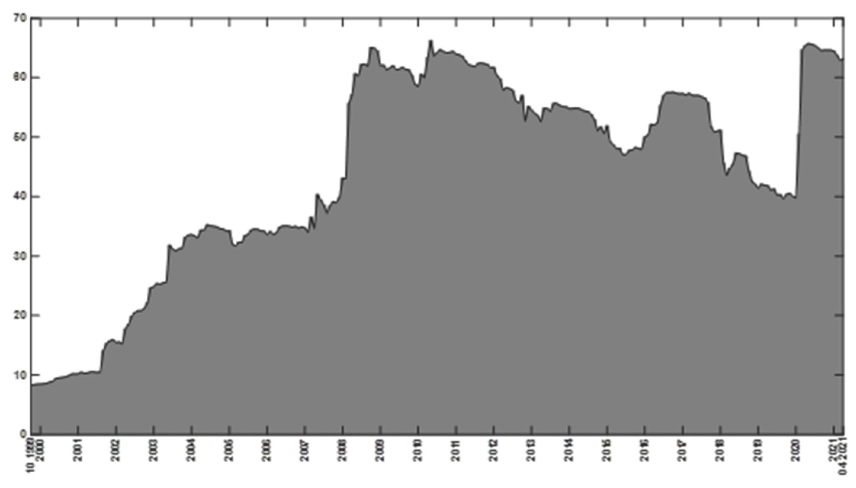
Spain is a small open economy, and therefore the events that trigger the dynamics of the total stress connectedness are also shaped by external factors. In this section, we conduct a robustness exercise studying the connectedness between the stress composite indices for the peripheral EA economies, i.e., Greece, Portugal, Spain, and Italy.12 To do so, we download from the European Central Bank’s website13 the monthly Composite Indicator of Systemic Stress (CISS) from January 1999 to April 2021. This index is the European equivalent to the composite stress index of Spain explained in Section 3. We calculate and plot in Figure 3 the dynamic total stress connectedness of the peripheral EA economies.14
Figure 3 shows that there has been a persistent increase in the connectedness between the peripheral EA financial markets’ stress indices since the beginning of the sample. This suggests that the peripheral EA markets have become more integrated. More importantly, and despite the sample differences with Figure 2, one can observe some similarities between the dynamic total stress connectedness among the Spanish financial markets and that of the peripheral EA composite stress indices. Namely, the total stress connectedness of the peripheral EA countries climbed from 35% to close to 65% during the GFC (2008), stayed high during the European sovereign debt crisis (2010), and then decreased afterwards. Additionally, the connectedness increased strongly at the beginning of the COVID-19 pandemic crisis in February–March 2020. In sum, we can conclude that the external variables that shaped the dynamics of the total stress connectedness among the Spanish financial markets are also shaping that of the peripheral EA composite stress indices. Our findings are consistent with earlier literature in that the linkage between markets intensifies during periods of increasing economic and financial instability (see, e.g., Kolb 2011), implying a loss of diversification just when it is needed most. In this respect, some authors have argued that a crisis in one country may give a “wake up call” to international investors to reassess the risks in other countries, thereby generating excess co-movements across the markets (see Beirne and Fratzscher 2013).
5. Net Directional Connectedness
5.1. Net Directional Stress Connectedness Plots
The net directional connectedness index provides information about how much each market segment’s stress contributes in net terms to other segments. This analysis can help us to determine which markets are net transmitters or net recipients of spillovers. The net directional spillovers across all stress indices under study are calculated by subtracting directional “to others” from directional “from others”. Therefore, the positive (negative) values indicate a source (recipient) of stress transmission to (from) other market indices. As with the dynamic total connectedness measure presented in Section 4.2, this also relies on the TVP-VAR connectedness approach. Figure 4 displays the dynamic net connectedness.
As shown in Figure 4, most of the stress indices under investigation appear to frequently switch between assuming a net transmitting and a net receiving role of financial stress, except for the index representing the derivatives market (light blue line), which is a recipient of stress throughout 96.10% of the sample (with its estimated average value for net directional connectedness being −16.24%). This result suggests that the derivatives market is not a trigger of stress to the system, as is usually suggested in the financial press (Warren Buffet called derivatives markets “financial weapons of mass destruction”), but rather a receiver of stress from underlying markets. Thus, these net directional connectedness relationships are bidirectional and asymmetric across five of the six stress indices. Moreover, our results suggest that the foreign exchange market (green line) and the bond market (black line) are net absorbers of financial stress throughout the sample (showing negative values for 68.60% and 57.85% of the sample, respectively, and with average values of −2.33% and −1.13%, respectively), while the financial intermediaries (red line), the money market (yellow line), and the equity market (dark blue line) are net stress propagators during most of the sample (rending positive values for 86.38%, 63.40%, and 61.06% of the sample, respectively, with average values of 12.52%, 2.80%, and 4.39%, respectively).
Interestingly, financial intermediaries have been the largest generators of stress in the Spanish financial markets by far. This result may be explained by the major role of the banking sector in the Spanish financial system (see for example Malo de Molina and Martín-Aceña 2012).
A further inspection of Figure 4 indicates the existence of at least two significant subperiods of intense transmission of stress from the five stress indicators to the derivatives market stress indicator: (i) from August 2007 to October 2008, which coincides with the GFC; (ii) from early 2020 until the end of the sample, with an intense period of stress received during the outbreak of the COVID-19 pandemic (March to June 2020). We will study these and other extraordinary stress periods in greater detail in the next subsection.
5.2. Dynamic Net Pairwise Directional Stress Connectedness Plots
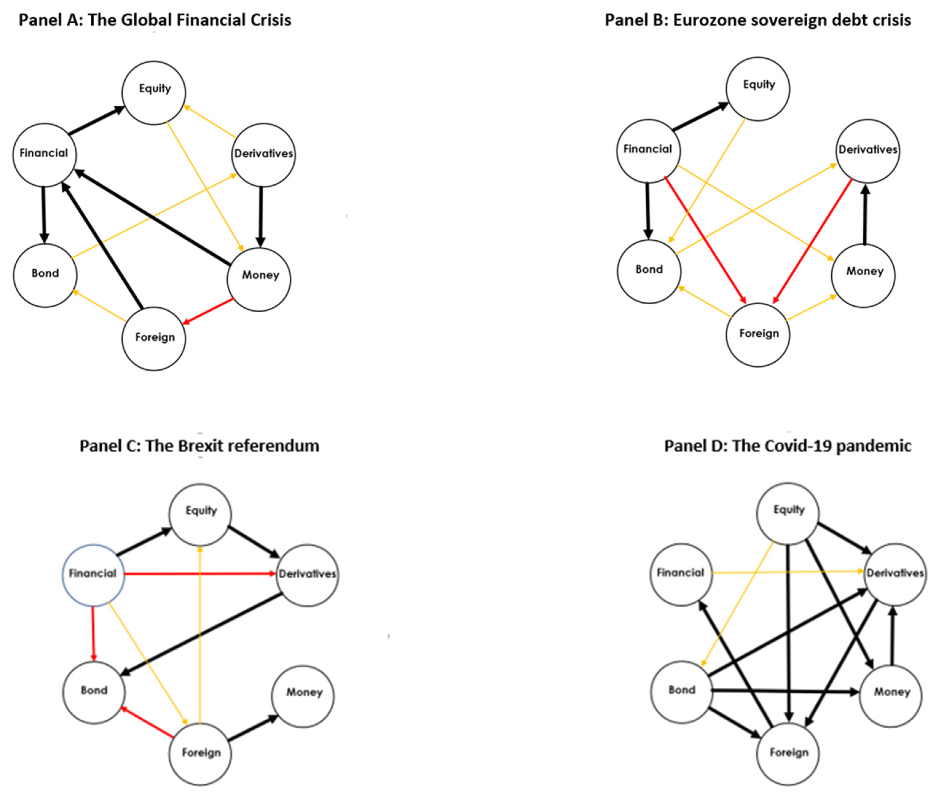
So far, we have discussed the behaviour of the total connectedness and total net directional connectedness measures for the six indices representative of the Spanish financial market segments. We now turn our attention to the net pairwise directional connectedness in order to shed some light on the key transmitters and receivers of shocks in a bivariate setting. Figure 5 displays the network plots for certain critical periods in the sample period to visualise the time-varying propagation of stress between the market segments currently under consideration.15 In particular, panels A to D in Figure 5 display net pairwise directional stress connectedness during four major events affecting the Spanish economy that were previously identified in the stress indices (c.f. Figure 1). These are: (i) the GFC (from August 2007 to October 2008);16 (ii) the EA sovereign debt crisis (April 2010 to August 2011);17 (iii) the financial turmoil after the Brexit referendum (June to October 2016);18 (iv) the COVID-19 outbreak (March to June 2020).19
The six nodes in Figure 5 represent the six stress indices. The arrow connecting the nodes represents the information spillover direction from one index to another, being equal to the net pairwise connectedness measures between the two nodes. The colour of the arrows indicates the strength of connectedness between stress index pairs, from the strongest to the weakest. We used three colour codes (black, red, and orange links, or black, grey, and light grey when viewed in greyscale) that represent the 90th, 80th, and 70th percentiles of all net pairwise directional connections (i.e., the highest values of the 15 measures of intensity of the pairwise connectedness between the six stress indices being examined in that particular period).
As can be seen, during the GFC (panel A), the net pairwise connectedness plot differs from that obtained for the static pairwise connectedness measures, confirming once again the importance of the dynamic connectedness. In particular, the derivatives market is identified in this pairwise analysis as the dominant transmitter of stress to the money segment, while the latter and the foreign market are net stress triggers of the financial intermediaries, which in turn are a net transmitter of stress to the equity and bond markets. Considering all the segments, the financial intermediaries were the main triggers of stress during the global financial crisis, with two black arrows pointing toward two stress indicators. This result can be associated with the fact that Spain’s banking system was clearly excessively large at the time, over-concentrated on lending funds to real estate and residential construction activities, and highly dependent on international wholesale financing (see for example Hernández de Cos 2019), as well as significantly affected by the turmoil that arose from the growing U.S. subprime mortgage default rate. The EA sovereign debt crisis exerted a similar pattern (panel B). The financial intermediaries were again the main net transmitter of stress to all segments except derivatives markets, and particularly to the equity and bond markets. This result reflects the key role played by the sovereign bank nexus in the European debt crisis, enabling pernicious dynamics whereby governments and domestic banking sectors mutually weakened each other (Gomez-Puig et al. 2019).20 Moreover, during this episode, the money market becomes a significant net generator to the derivatives market. Regarding the shock originated by the Brexit decision (panel C), the pairwise directional stress spillovers are particularly strong from financial intermediaries to equities, from equities to derivatives, from derivatives to bonds, and from foreign exchanges to money markets. The two main generators of stress in the Spanish financial system during the Brexit episode are the financial intermediaries (a net generator of stress to all segments but the money market) and the foreign exchange market (a net generator of stress to all segments but financial intermediaries and derivatives markets). These findings confirm that Brexit-induced policy uncertainty caused financial instability in key financial markets (Bloom et al. 2018), given the prospect of considerably long negotiations (Philippon 2016) and the perception of potential damage to the real economy in both the UK and other European countries (Belke et al. 2018). In this sense, our results capture the strong connections with the United Kingdom in terms of both trade and tourism and interrelationships with the financial sector, with Spanish banks having the largest investments of any European country in the UK’s private banking sector (Carbó-Valverde and Rodríguez-Fernández 2017). Finally, analysis of the COVID-19 pandemic (panel D) reveals a completely different picture as compared to the previous three crises. There is an intricate network of vigorous interrelations among all market segments under study. This result is in line with the fact that in May 2020, the Spanish Financial Market Stress Indicator registered the highest rebound in its history over a cumulative period of a few weeks, reaching its third-highest maximum since 1999 and with an increase in the degree of correlation between all of its segments. From this highly interconnected network, the main generators of stress during the COVID-19 pandemic crisis have been the equity market (with strong links to all segments but financial intermediaries) and the bond markets (with strong links to derivatives, money, and foreign exchange markets). Interestingly, the major difference in the interactions between the Spanish stress indices during the COVID-19 pandemic crisis and the previous three financial crisis is the role of the financial intermediaries. Specifically, the financial intermediaries have played a different role during the COVID-19 pandemic crisis, serving as mild generators of stress to derivatives markets only. This result can be explained by the gradual process of increasing the strength and solvency of the Spanish banking system by way of the Fund for Orderly Bank Restructuring launched in 2009, with significant advances during the 2012–2016 period (International Monetary Fund 2017). This contributed to a healthier position of the financial intermediaries during the COVID-19 pandemic crisis period, gradually reducing the role of financial intermediaries as stress transmitters to the remaining market segments as compared to prior crises.
In summary, the financial intermediaries segment was the major generator of stress to the Spanish financial system during the GFC, the Eurozone sovereign debt crisis, and the global financial turmoil following the Brexit referendum, but during the COVID-19 pandemic crisis, the equity and bond markets were the major generators of stress to the system. Overall, these findings corroborate that the number and intensity of pairwise stress spillover effects across the examined market segments experience noteworthy increases during financial turbulences. These results also highlight special relevance in the case of the COVID-19 disturbance, which has contracted the levels of activity in Spain on a scale never before witnessed in peacetime and has damaged the Spanish financial system substantially.
6. Concluding Remarks
The purpose of this paper was to analyse the total, pairwise, and net pairwise connectedness between six stress indicators representative of the Spanish financial market segments by employing both the Diebold and Yilmaz (2012) methodology and the modified approach of Antonakakis et al. (2018). We also constructed the network of stress connectedness to capture the propagation path of recent crisis shocks across the market segments.
The main findings are summarised as follows. In the first step, we found a system-wide value of 15.67% for the total connectedness between the six stress indices under study for the full sample period, indicating that the remainder (84.33% of the variation) was due to idiosyncratic shocks. In the second step, we analysed the dynamic nature of the total connectedness, obtaining evidence of strong spillovers between market segments with large variations over time. This finding supports the literature documenting that stress transmission across market segments increases during times of financial turbulence. Moreover, our results suggest that high levels of pandemic and economy policy uncertainty and real economy deterioration are the main drivers of the detected total dynamic connectedness. In a third step, we examined the time-varying net spillovers across stress indices. Across all major financial crises in the recent history of the Spanish economy, we identified the financial intermediaries segment as the principal generator of stress to the Spanish financial system, although the equity and bond markets triggered stress to the system during the COVID-19 pandemic crisis. This suggests a healthier position of the Spanish financial intermediaries during the COVID-19 pandemic crisis period, with these having gradually reduced their role as stress transmitters to the other market segments as compared to previous crises. Our results also indicate significant stress transfer between all market segments during the COVID-19 outbreak, vividly illustrating the impacts of unanticipated events.
These findings will be useful to portfolio managers, professional forecast analysts, and risk managers dealing with sector markets, as well as policymakers, who should take into consideration the spillover effects detected by the dynamic interdependences between the stress indices under study. Indeed, the connectedness measure can be used in a static or dynamic context to show the state of potential contagion among different market segments at a certain point in time. Our results reveal the importance of monitoring all market segments to assess financial contagion.
A natural extension of the analysis presented in this paper would be to explore the potential non-linearity in the relationship between the stress indices of the Spanish financial markets (e.g., through a kernel method), which could uncover more interesting dynamics in these relationships. This is an item in our future research agenda.
Author Contributions
J.A.-F.: software, formal analysis, data curation, visualisation, validation. A.F.-P.: investigation, methodology, software, formal analysis. S.S.-R.: conceptualisation, methodology, writing—original draft preparation, writing—review and editing, validation. All authors have read and agreed to the published version of the manuscript.
Funding
This research was funded by the Spanish Ministry of Science and Innovation under grant PID2019-105986GB-C21; Generalitat de Catalunya under grant 2020PANDE00074; and Cabildo Insular de Gran Canaria under grant CABILDO2018-03.
Data Availability Statement
Primary data supporting reported results can be found at the Spanish National Securities Market Commission (CNMV) website: http://www.cnmv.es/Portal/home.aspx (accessed on 9 April 2021).
Acknowledgments
The authors wish to thank two anonymous referees and the editor for their insightful comments and suggestions on a previous draft of this paper. They are also very grateful to Gary Koop and Dimitris Korobilis for providing the TVP-VAR programs.
Conflicts of Interest
The authors declare no conflict of interest.
| 1 | |
| 2 | Note that the Diebold and Yilmaz (2014)’s approach assumes a linear relationship between the variables under study. An alternative approach would be to consider non-linear relationships, but Granger (2008) argues that economic interpretations of non-linear models are difficult. Furthermore, based on the White’s theorem, Granger (2008) shows that any non-linear model can be approximated by a time-varying parameter (TVP) linear model. In the spirit of the family of models described in Granger (2008), we complement our analysis by applying the dynamic connectedness procedure based on the TVP-VAR proposed by Antonakakis et al. (2018) that renders both an optimal approximation of general non-linear processes and more readily interpretable results. |
| 3 | Following Koop and Korobilis (2014), we use the same non-informative initial conditions in the Kalman filter, a decay factor of 0.96, and a forgetting factor of 0.99 (see online Appendix in Koop and Korobilis 2014, for the technical details). Without loss of generality, we normalise the series to get a faster and smoother convergence in the Kalman filter. This normalisation does not have any effect on the connectedness matrix. |
| 4 | All results are based on a VAR model of order 2 and generalised variance decompositions of 10-week-ahead forecast error. To check for the sensitivity of the results to the choice of the order of VAR, we also calculate the spillover index for orders 2 through 4, as well as for forecast horizons ranging from 4 weeks to 10 weeks. The main results of our paper are not affected by these choices. Detailed results are available from the authors upon request. |
| 5 | We are grateful to two anonymous referees for suggesting this exploratory analysis. |
| 6 | The WUI is computed by counting the percent of word “uncertain” (or its variant) in the Economist Intelligence Unit country reports [see https://worlduncertaintyindex.com/data/] (accessed on 14 October 2021). |
| 7 | The World Pandemic Uncertainty Index (WPUI) measures uncertainty related to pandemics across the globe [see https://worlduncertaintyindex.com/data/] (accessed on 14 October 2021). The Pearson correlation between the WPUI Global and the WPUI-Spain is high (0.93), and therefore, we decide to use only the Spain’s component to avoid multicollinearity issues in the regressions. We also consider the number of COVID-19 cases in Spain, Europe and worldwide using data from European Centre for Disease Prevention and Control, but these series were highly correlated with WPUI-Spain. |
| 8 | This measure is constructed by counting the number of U.S. newspaper articles achieved by the NewsBank Access World News database with at least one term from each of the following three categories: (i) “economic” or “economy”; (ii) “uncertain” or “uncertainty”; and (iii) “legislation,” “deficit,” “regulation,” “congress,” “Federal Reserve,” or “White House.” Baker et al. (2016) provide evidence that EPU captures perceived economic policy uncertainty. Ghirelli et al. (2019) replicate their results for Spain. See https://www.policyuncertainty.com/spain.html (accessed on 14 October 2021). |
| 9 | |
| 10 | A cubic spline curve is a mathematical representation of piecewise third-order polynomials passing through a set of k control points and subject to boundary conditions (De Boor 1978). This has been extensively used in the literature when the frequency of series do not match (see e.g., Bauwens and Hautsch 2009). |
| 11 | To that end we perform a variety of unit root tests. The results, which are not shown here in order to save space, are available from the authors upon request. |
| 12 | We are grateful to an anonymous referee for suggesting this robustness analysis. |
| 13 | See https://sdw.ecb.europa.eu/browseExplanation.do?node=9693347 (accessed on 14 October 2021). |
| 14 | The static connectedness table between the peripheral EA financial stress indices suggests that the stress of the Spanish financial markets is highly connected to those of the peripheral EA financial markets. Specifically, there are high gross pairwise directional connectedness from Spain to Italy (25.37%) and vice versa (20.36%), and from Spain to Portugal (19.41%) and vice versa (28.08%). These additional results are not shown here to save space, but they are available from the authors upon request. |
| 15 | To save space, the results of the decomposition of the dynamic net directional connectedness into their pairwise directional connectedness for each stress are not shown here, but they are available from the authors upon request. |
| 16 | We consider the period between the announcement by the French investment bank BNP Paribas that it was suspending three investment funds (9 August 2007) to the coordinated Central Bank actions taken to address pressures in global money markets (8 October 2008). |
| 17 | We consider the period of maximum turbulence in the Eurozone sovereign debt markets, covering the rescue packages not only in Greece (May 2010), but also in Ireland (November 2010) and Portugal (April 2011); Additionally, the ECB announced in August 2011 its second covered bond purchase programme. |
| 18 | We consider the period from the United Kingdom’s decision by referendum to leave the European Union (23 June 2016) to the announcement by Prime Minister Theresa May to trigger the EU’s Article 50—the mechanism to set the formal exit process in motion (2 October 2016). |
| 19 | By 13 March 2020, COVID-19 cases had been confirmed in all 50 Spanish provinces, and the next day the government declared a state of emergency, which ended on 21 June 2020, after three months of lockdown. The lockdown measures in Spain were among the strictest in Europe. |
| 20 | After severe pressure in European sovereign debt markets, in July 2012 Spain turned to the European Union for help to ensure the solvency of its banking sector, signing a Memorandum of Understanding that led to the implementation of a series of corrective, preventive, and proactive measures that were supervised and monitored until the end of 2015. |
References
- Antonakakis, Nikolaos, David Gabauer, Rangan Gupta, and Vasilios Plakandaras. 2018. Dynamic connectedness of uncertainty across developed economies: A time-varying approach. Economics Letters 166: 63–75. [Google Scholar] [CrossRef] [Green Version]
- Arsov, Ivalio, Elie Canetti, Laura Kodres, and Srobona Mitra. 2013. ‘Near-Coincident’ Indicators of Systemic Stress. Working Paper 13/115. Washington, DC: International Monetary Fund. [Google Scholar]
- Baele, Lieven, Geert Bekaert, Koen Ingelbrecth, and Min Wei. 2020. Flights to Safety. Review of Financial Studies 33: 689–746. [Google Scholar] [CrossRef]
- Baker, Scott, Nicholas Bloom, and Steven Davis. 2016. Measuring economic policy uncertainty. Quarterly Journal of Economics 131: 1593–636. [Google Scholar] [CrossRef]
- Bauwens, Luc, and Nikolaus Hautsch. 2009. Modelling Financial High Frequency Data Using Point Processes. Edited by Thomas Mikosch, Jens-Peter Kreiß, Richard Davis and Torben Gustav Andersen. Handbook of Financial Time Series; Berlin: Springer. [Google Scholar]
- Beirne, John, and Marcel Fratzscher. 2013. The pricing of sovereign risk and contagion during the European sovereign debt crisis. Journal of International Money and Finance 34: 60–82. [Google Scholar] [CrossRef] [Green Version]
- Belke, Ansgar, Irina Dubova, and Thomas Osowski. 2018. Policy uncertainty and international financial markets: The case of Brexit. Applied Economics 50: 3752–70. [Google Scholar] [CrossRef] [Green Version]
- Bloom, Nicholas, Philip Bunn, Scarlet Chen, Paul Mizen, Pawel Smietanka, Greg Thwaites, and Garry Young. 2018. Brexit and uncertainty: Insights fom the Decision Maker Panel. Fiscal Studies 39: 555–80. [Google Scholar] [CrossRef]
- Caldarelli, Roberto, Selim Elekdag, and Subir Lall. 2011. Financial stress and economic contractions. Journal of Financial Stability 7: 78–97. [Google Scholar] [CrossRef]
- Carbó-Valverde, Santiago, and Francisco Rodríguez-Fernández. 2017. Outlook for the Spanish financial sector ahead of Brexit. Spanish and International Economic and Financial Outlook 6: 53–61. [Google Scholar]
- Chen, Xiaoyu, and Thomas Chiang. 2020. Empirical investigation of changes in policy uncertainty on stock returns: Evidence from China’s market. Research in International Business and Finance 53: 101183. [Google Scholar] [CrossRef]
- Cogley, Thimoty, and Thomas Sargent. 2005. Drifts and volatilities: Monetary policies and outcomes in the post WWII US. Review of Economic Dynamics 8: 262–302. [Google Scholar] [CrossRef] [Green Version]
- De Boor, Carl. 1978. A Practical Guide to Splines. New York: Springer. [Google Scholar]
- Diebold, Francis Xavier, and Kamil Yilmaz. 2012. Better to give than to receive: Predictive directional measurement of volatility spillovers. International Journal of Forecasting 28: 57–66. [Google Scholar] [CrossRef] [Green Version]
- Diebold, Francis Xavier, and Kamil Yilmaz. 2014. On the network topology of variance decompositions: Measuring the connectedness of financial firms. Journal of Econometrics 182: 119–34. [Google Scholar] [CrossRef] [Green Version]
- Gabauer, David, and Rangan Gupta. 2018. On the transmission mechanism of country specific and international economic uncertainty spillovers: Evidence from TVP-VAR connectedness decomposition approach. Economics Letters 171: 63–71. [Google Scholar] [CrossRef] [Green Version]
- Ghirelli, Corinna, Javier Perez, and Alberto Urtasun. 2019. A new economic policy uncertainty index for Spain. Economic Letters 182: 64–67. [Google Scholar] [CrossRef] [Green Version]
- Gomes, Francisco, Laurence Kotlikoff, and Luis Viceira. 2012. The excess burden of government indecision. Tax Policy and the Economy 26: 125–64. [Google Scholar] [CrossRef] [Green Version]
- Gomez-Puig, Marta, Manish Singh, and Simón Sosvilla-Rivero. 2019. The sovereign-bank nexus in peripheral euro area: Further evidence from contingent claims analysis. North American Journal of Economics and Finance 49: 1–46. [Google Scholar] [CrossRef]
- Granger, Clive William John. 2008. Non-linear models: Where do we go next—Time varying parameter models? Studies in Nonlinear Dynamics and Econometric 12: 1639. [Google Scholar] [CrossRef]
- Hernández de Cos, Pablo. 2019. The Spanish banking system: Transformations and challenges. Paper presented at Sustainable Finances and Their Importance in the Future of the Economy, Madrid, Spain, Universidad Internacional Menéndez Pelayo, Spanish Association of Economics Journalists. June 17. [Google Scholar]
- Holló, Danial, Mamfred Kremer, and Marco Lo Duca. 2012. CISS—A Composite Indicator of Systemic Stress in the Financial System. Working Paper 1426. Frankfurt upon Main: European Central Bank. [Google Scholar]
- Illing, Mark, and Ying Liu. 2006. Measuring financial stress in a developed country: An application to Canada. Journal of Financial Stability 2: 243–65. [Google Scholar] [CrossRef]
- International Monetary Fund. 2017. Financial System Stability Assessment. Washington, DC: Spain International Monetary Fund. [Google Scholar]
- Kolb, Robert. 2011. Financial Contagion: The Viral Threat to the Wealth of Nations. Hoboken: John Wiley & Sons. [Google Scholar]
- Koop, Gary, and Dimitris Korobilis. 2014. A new index of financial conditions. European Economic Review 71: 101–16. [Google Scholar] [CrossRef] [Green Version]
- Koop, Gary, Mohammad Hashem Pesaran, and Simon Potter. 1996. Impulse response analysis in non-linear multivariate models. Journal of Econometrics 74: 119–47. [Google Scholar] [CrossRef]
- Kremer, Manfred. 2016. Macroeconomic effects of financial stress and the role of monetary policy: A VAR analysis for the euro area. International Economics and Economic Policy 13: 105–38. [Google Scholar] [CrossRef]
- Krippner, Leo. 2013. Measuring the stance of monetary policy in zero lower bound environments. Economics Letters 11: 135–38. [Google Scholar] [CrossRef] [Green Version]
- Kritzman, Mark, Yaunzhen Li, Mark Kritzman, and Roberto Rigobon. 2011. Principal components as a measure of systemic risk. Journal of Portfolio Management 37: 112–26. [Google Scholar] [CrossRef] [Green Version]
- Li, Xiaoming, Bing Zhang, and Ruzhao Gao. 2015. Economic policy uncertainty shocks and stock–bond correlations: Evidence from the US market. Economics Letters 132: 91–96. [Google Scholar] [CrossRef]
- Malo de Molina, José Luis, and Pablo Martín-Aceña. 2012. The Spanish Financial System. Basingstoke: Palgrave Macmillan. [Google Scholar]
- Mei, Dexiang, Qing Zeng, Yaojie Zhang, and Wenjing Hou. 2018. Does US Economic Policy Uncertainty matter for European stock markets volatility? Physica A: Statistical Mechanics and Its Applications 512: 215–21. [Google Scholar] [CrossRef]
- Nelson, William, and Roberto Perli. 2007. Selected indicators of financial stability. Irving Fisher Committee’s Bulletin on Central Bank Statistics 23: 92–105. [Google Scholar]
- Pástor, Lubios, and Pietro Veronesi. 2012. Uncertainty about government policy and stock prices. Journal of Finance 67: 1219–64. [Google Scholar] [CrossRef]
- Pástor, Lubios, and Pietro Veronesi. 2013. Political uncertainty and risk premia. Journal of Financial Economics 110: 520–45. [Google Scholar] [CrossRef] [Green Version]
- Pesaran, Mohammad Hashem, and Yongcheol Shin. 1998. Generalized impulse response analysis in linear multivariate models. Economics Letters 58: 17–29. [Google Scholar] [CrossRef]
- Philippon, Thomas. 2016. Brexit and the End of the Great Policy Moderation. Brookings Papers on Economic Activity 2: 385–93. [Google Scholar] [CrossRef]
- Wisniewski, Tomasz Piotr, and Brendan John Lambe. 2015. Does economic policy uncertainty drive CDS spreads? International Review of Financial Analysis 42: 447–58. [Google Scholar] [CrossRef] [Green Version]
Figure 1.
Stress indicators of the Spanish financial markets.


Figure 2.
Dynamic total connectedness for stress indicators of the Spanish financial market. Note: The predictive horizon for the underlying variance decomposition is 10 weeks.
Figure 2.
Dynamic total connectedness for stress indicators of the Spanish financial market. Note: The predictive horizon for the underlying variance decomposition is 10 weeks.

Figure 3.
Dynamic total connectedness of the EA peripheral countries’ CLIFS values.

Figure 4.
Net directional connectedness for stress indicators of the Spanish financial market.


Figure 5.
Network diagram of pairwise net directional stress spillovers on certain critical episodes. Note: We show the most important net directional connections among the six market stress indices under study for four critical episodes. Panel (A) illustrates the period of the global financial crisis (August 2007 to October 2008), panel (B) shows the Eurozone sovereign debt crisis (April 2010 to August 2011), panel (C) shows the global financial turmoil following the Brexit referendum (June to October 2016), and panel (D) shows the outbreak of the COVID-19 pandemic (March to June 2020). Black, red, and orange links (black, grey, and light grey when viewed in greyscale) correspond respectively to the 90th, 80th, and 70th percentiles of all net pairwise directional connections.


Table 1.
Schematic connectedness table.
| … | Connectedness FROM Others | ||||
|---|---|---|---|---|---|
| … | |||||
| … | |||||
| … | |||||
| Connectedness to Others | … | Total connectedness |
Table 2.
Descriptive statistics and contemporaneous correlations of the stress indices.
| Panel A: Descriptive Statistics | ||||||
| Bond Market | Equity Market | Financial Intermediaries | Foreign Exchange Market | Derivatives Market | Money Market | |
| Mean | 0.5006 | 0.4170 | 0.5416 | 0.5251 | 0.4935 | 0.4383 |
| Median | 0.5280 | 0.4025 | 0.5395 | 0.5225 | 0.4830 | 0.4020 |
| Minimum | 0.0250 | 0.0040 | 0.0120 | 0.0090 | 0.0760 | 0.0000 |
| Maximum | 0.9960 | 0.9620 | 1.0000 | 0.9990 | 0.9740 | 0.9980 |
| Std. Dev. | 0.2316 | 0.2226 | 0.2408 | 0.2152 | 0.1708 | 0.2115 |
| Skewness | 0.0068 | 0.2070 | −0.1397 | 0.0561 | 0.3595 | 0.6760 |
| Excess kurtosis | −0.9376 | −0.9468 | −0.8733 | −0.6481 | −0.1161 | −0.1995 |
| Jarque-Bera | 42.58 a | 51.70 a | 40.71 a | 20.95 a | 25.69 a | 90.41 a |
| p-value | (0.0010) | (0.0010) | (0.0010) | (0.0010) | (0.0010) | (0.0010) |
| Observations | 1162 | 1162 | 1162 | 1162 | 1162 | 1162 |
| Panel B: Matrix Correlations | ||||||
| Bond Market | Equity Market | Financial Intermediaries | Foreign Exchange Market | Derivatives Market | Money Market | |
| Bond market | 1.0000 | |||||
| Equity market | 0.2385 a (0.0000) | 1.0000 | ||||
| Financial intermediaries | 0.6523 a (0.0000) | 0.5355 a (0.0000) | 1.0000 | |||
| Foreign exchange market | 0.1283 a (0.0000) | 0.4273 a (0.0000) | 0.2812 a (0.0000) | 1.0000 | ||
| Derivatives market | 0.2183 a (0.0000) | 0.5644 a (0.0000) | 0.4663 a (0.0000) | 0.3609 a (0.0000) | 1.0000 | |
| Money market | −0.0453 (0.1228) | 0.3587 a (0.0000) | 0.2028 a (0.0000) | 0.2552 a (0.0000) | 0.3529 a (0.0000) | 1.0000 |
Notes: Weekly data from 1 January 1999 to 2 April 2021; a indicates significance at the 1% level.
Table 3.
Full-sample connectedness.
| Bond Market | Equity Market | Financial Intermediaries | Foreign Exchange Market | Derivatives Market | Money Market | Directional From Others | |
|---|---|---|---|---|---|---|---|
| Bond market | 93.13 | 1.77 | 3.10 | 1.00 | 0.86 | 0.13 | 6.87 |
| Equity market | 2.44 | 76.87 | 9.61 | 6.18 | 2.59 | 2.31 | 23.13 |
| Financial intermediaries | 2.52 | 6.24 | 85.89 | 2.06 | 1.06 | 2.25 | 14.11 |
| Foreign exchange market | 1.63 | 6.41 | 1.94 | 85.68 | 2.58 | 1.75 | 14.32 |
| Derivatives market | 1.26 | 13.21 | 7.26 | 3.76 | 69.46 | 5.05 | 30.54 |
| Money market | 0.19 | 1.61 | 0.83 | 1.30 | 1.15 | 94.94 | 5.06 |
| Directional to others | 8.03 | 29.24 | 22.73 | 14.31 | 8.23 | 11.49 | Total connectedness = 15.67 |
| net contribution (to–from) others | 1.16 | 6.11 | 8.62 | −0.01 | −22.31 | 6.43 |
Table 4.
Determinants of the dynamic total connectedness.
| (1) | (2) | (3) | ||||
| Constant | 0.01 | (0.38) | 0.01 | (0.41) | 0.01 | (0.41) |
| Lagged Total Connectedness | 0.85 a | (25.17) | 0.86 a | (31.10) | 0.84 a | (24.75) |
| Uncertainty indicators | ||||||
| WUI Global | −0.02 | (−0.47) | −0.03 | (−1.08) | ||
| WUI-Spain | 0.03 | (1.06) | 0.02 | (0.96) | ||
| WPUI-Spain | 0.11 b | (2.01) | 0.10 a | (2.52) | ||
| ΔEPU-Spain | 0.11 c | (1.90) | 0.10c | (1.80) | ||
| Economic activity indicators | ||||||
| ΔIPI (%) | −0.08 c | (−1.81) | −0.05 b | (−2.38) | ||
| ΔGDP (%) | −0.09 a | (−2.59) | −0.07 a | (−3.28) | ||
| ΔSSR | −0.03 | (−0.81) | −0.04 | (−1.06) | ||
| Adj-R² (%) | 79.60 | 78.79 | 80.31 | |||
Note: This table reports the estimation results of Equation (13). Newey–West corrected t-statistics are reported in parenthesis. The sample is from March 1999 to April 2021; a,b,c represent significance at the 1%, 5%, and 10% levels, respectively.
Publisher’s Note: MDPI stays neutral with regard to jurisdictional claims in published maps and institutional affiliations. |
© 2021 by the authors. Licensee MDPI, Basel, Switzerland. This article is an open access article distributed under the terms and conditions of the Creative Commons Attribution (CC BY) license (https://creativecommons.org/licenses/by/4.0/).
Share and Cite
MDPI and ACS Style
Andrada-Félix, J.; Fernandez-Perez, A.; Sosvilla-Rivero, S. Stress Spillovers among Financial Markets: Evidence from Spain. J. Risk Financial Manag. 2021, 14, 527. https://0-doi-org.brum.beds.ac.uk/10.3390/jrfm14110527
AMA Style
Andrada-Félix J, Fernandez-Perez A, Sosvilla-Rivero S. Stress Spillovers among Financial Markets: Evidence from Spain. Journal of Risk and Financial Management. 2021; 14(11):527. https://0-doi-org.brum.beds.ac.uk/10.3390/jrfm14110527
Chicago/Turabian StyleAndrada-Félix, Julián, Adrian Fernandez-Perez, and Simón Sosvilla-Rivero. 2021. "Stress Spillovers among Financial Markets: Evidence from Spain" Journal of Risk and Financial Management 14, no. 11: 527. https://0-doi-org.brum.beds.ac.uk/10.3390/jrfm14110527