Kernel Regression Coefficients for Practical Significance

Abstract

Quantitative researchers often use Student’s t-test (and its p-values) to claim that a particular regressor is important (statistically significantly) for explaining the variation in a response variable. A study is subject to the p-hacking problem when its author relies too much on formal statistical significance while ignoring the size of what is at stake. We suggest reporting estimates using nonlinear kernel regressions and the standardization of all variables to avoid p-hacking. We are filling an essential gap in the literature because p-hacking-related papers do not even mention kernel regressions or standardization. Although our methods have general applicability in all sciences, our illustrations refer to risk management for a cross-section of firms and financial management in macroeconomic time series. We estimate nonlinear, nonparametric kernel regressions for both examples to illustrate the computation of scale-free generalized partial correlation coefficients (GPCCs). We suggest supplementing the usual p-values by “practical significance” revealed by scale-free GPCCs. We show that GPCCs also yield new pseudo regression coefficients to measure each regressor’s relative (nonlinear) contribution in a kernel regression.

1. Introduction and Avoiding p-Hacking with Enhanced Regression Tools

Consider a usual ordinary least squares (OLS) linear regression with normal homoscedastic errors:

$$x_{1t}={\alpha }_{11}+{\mathsf{\Sigma }}_{i=2}^p{\alpha }_{1i}{x}_{it}+{ϵ}_t,{ϵ}_t\sim N(0,{\sigma }^2).$$

(1)

The estimated numerical magnitudes of p regression coefficients ${\widehat{\alpha }}_{1i}$ are sensitive to units of measurement of the variables $x_{it}$. The assumption of normally distributed errors ${ϵ}_t$ implies that the sampling distribution of ${\widehat{\alpha }}_{1i}$ defined over all possible samples of data follows the Student’s t density, see Kendall and Stuart (1977). A coefficient is statistically significantly different from zero if the p-value is less than 0.05 at the usual 95% level.

The p-hacking problem recently discussed in Wasserstein et al. (2019), Brodeur et al. (2020), and others associated with (1) occur when too many p-values in published papers are just below 0.05. The regression literature is too vast to cite; even papers related to p-hacking exceed 80. In a Special Issue of the American Statistician, Wasserstein and others suggest the following actions (among many others) for avoiding p-hacking: (i) Do not conclude anything about scientific or practical importance based on statistical significance (or lack thereof); (ii) accept uncertainty, and be thoughtful, open, and modest, or the acronym ATOM; and (iii) measure the size of what is at stake instead of the falsification of a null hypothesis.

This paper suggests new tools for implementing these actions, such as wider acceptance of nonlinear nonparametric kernel regressions. Since nonparametric means no coefficients as parameters, their p-values do not exist. How to interpret and explain the estimated kernel regression to the public remains a challenge. One can explain the kernel regression in terms of the estimated partial derivatives of the dependent variable with respect to regressors as coefficients. This paper suggests new pseudo-regression coefficients for Nadaraya–Watson kernel regressions using generalized (partial) correlations allowing for nonlinear relations.

We use scale-free generalized partial correlation coefficients (GPCCs) mentioned in Vinod (2021a) (without the acronym) to develop our pseudo regression coefficients. Hence, let us begin by reviewing well-known relations between scale-free partial correlation coefficients, scale-free so-called standardized beta coefficients, and usual OLS linear regression coefficients.

We distinguish between (a) the practical numerical significance of a regressor in explaining the variation in the dependent variable, and (b) its statistical significance measured by the t-test based on the sampling distribution of the regression coefficient over the population of all-possible data samples. Hirschauer et al. (2021) emphasize sample selection problems with traditional inference. The t-test p-values (used by p-hackers) rely on the unverified assumption that errors $ϵ$ are normally distributed. If a researcher wants to assess whether the practical significance of $x_2$ exceeds that of $x_3$, it would be highly misleading to check the corresponding inequality among OLS estimates, ${\widehat{\alpha }}_{12}>{\widehat{\alpha }}_{13}$, because the numerical magnitudes of all OLS coefficient estimates can be almost arbitrarily changed by rescaling the variables. For example, if the regressor $x_{2t}$ in (1) is multiplied by 100, its regression coefficient ${\widehat{\alpha }}_{12}$ become multiplied by (1/100).

Since the 1950s, some researchers have described regression coefficients of a standardized model as “standardized beta coefficients” obtained when all variables are standardized to have zero mean and unit standard deviation. One uses the transformation $x_{si}=(x_i-{\overline{x}}_i)/s_{xi}$ for all i, where $s_{xi}$ denotes the standard deviation (sd) of $x_i$. Ridge trace has standardized beta coefficients on the vertical axis and various biasing parameters $k\in [0,\infty )$ on the horizontal axis allowing a choice of k in a “stable region” of coefficients. The reporting of standardized beta coefficients has been so rare in recent decades that Wasserstein does not even mention it. We argue in favor of bringing back reporting standardized beta coefficients in addition to the p-values to discourage p-hacking. Lower panels of

Table 1. OLS estimation of a risk management model for ROA. Denoting standardized regressors with the ‘s’ suffix and forcing a zero intercept, lower panel ‘estimates’ suggest practical significance in a linear model.

	Estimate	Std. Error	t Value	Pr (>|t|)
(Intercept)	−1.4327	1.4109	−1.02	0.3107
RMC	−0.1665	0.1665	−1.00	0.3180
Lev	−0.2624	0.0709	−3.70	0.0003
Sale	4.0282	1.3209	3.05	0.0025
PCost	−1.3925	0.3217	−4.33	0.0000
OCost	−0.1530	0.1236	−1.24	0.2168
RMCs	−0.0561	0.0560	−1.00	0.3172
Levs	−0.1997	0.0538	−3.71	0.0002
Sales	0.1691	0.0553	3.05	0.0025
PCosts	−0.2494	0.0575	−4.34	0.0000
OCosts	−0.0733	0.0592	−1.24	0.2160

and

Table 2. OLS Results for Macro Example: money supply (m) regressed on prices, income, and interest rates. Denoting standardized regressors with the ‘s’ suffix and forcing a zero intercept, lower panel ‘estimates’ suggest practical significance in a linear model.

	Estimate	Std. Error	t Value	Pr (>|t|)
(Intercept)	−0.5830	0.0933	−6.25	0.0000
p	0.8090	0.0836	9.68	0.0000
y	1.1016	0.0725	15.20	0.0000
r	−0.0715	0.0074	−9.71	0.0000
ps	0.4491	0.0461	9.74	0.0000
ys	0.6255	0.0409	15.28	0.0000
rs	−0.1479	0.0151	−9.77	0.0000

illustrate their use for two examples discussed later.

Result 1

(Standardized Betas and Practical Significance). The magnitude of any particular standardized beta coefficient is comparable to that of any other standardized beta coefficient belonging to a regression model. Hence, numerical magnitudes of standardized beta coefficients represent an approximation to the “practical significance” of the regressor.

The regression model from (1) above in standardized units becomes:

$$x_{s1t}={\mathsf{\Sigma }}_{i=2}^p{\beta }_{1i}{x}_{sit}+{ϵ}_t.$$

(2)

The subtraction of each variable from its mean removes the intercept, making the true unknown intercept zero, or ${\beta }_{11}=0$. The software can force the estimate, ${\widehat{\beta }}_{11}$, to equal zero, except that such forcing slightly changes all slope coefficient estimates.

The effect of standardization is that all variables are measured in their own standard deviation (sd) units, making the magnitudes of variables and the corresponding coefficients comparable with each other. The practical significance computation is quite distinct from the statistical significance measured by p-values (and confidence intervals). We argue that the estimation of practical significance provides additional insights, helping safeguard against p-hacking.

The relation between the usual OLS slope coefficients (alpha) and corresponding standardized beta coefficients (all variables are standardized with zero mean and unit sd) is:

$${\widehat{\alpha }}_{1i}={\widehat{\beta }}_{1i}(s_{x1}/s_{sxi}),i=2,\dots ,p,$$

(3)

where the ‘sd’ (standard deviation) of the dependent variable is $s_{x1}$. We obtain the OLS slope coefficients from the standardized beta coefficients by multiplying by the ‘sd’ of the dependent variable and dividing by the regressor’s ‘sd.’ We shall use similar multiplications in the sequel to obtain our pseudo-regression coefficients from scale-free GPCCs, formally defined later in (15).

Steps for Better Modeling Strategies

A proper understanding of the newer methods, including GPCC, needs further definitions and mathematical notation. We shall formally discuss them in later sections with examples. This subsection provides a step-by-step preview of the proposed methods. We list R software commands (algorithms) selected from the R package generalCorr here. R being open source, any interested reader can see all steps inside each algorithm by simply typing its name. The following R commands often assume that the researcher has collected the data for all variables in a matrix denoted by ‘mtx,’ usually having the response variable in its first column:

• A regression specification usually requires that the variables on the right-hand side are ‘exogenous’ and approximately cause the response on the left-hand side, see Koopmans (1950). One can check if all right-hand side variables are ‘causal’ in some sense by issuing the command causeSummBlk(mtx). If the output of this command says that the response variable might be causing a regressor, the model specification is said to suffer from the endogeneity problem. Careful choice of the model for response and regressors will require accepting uncertainty while remaining thoughtful (causal variables as regressors), open (to alternate specifications), and modest, (ATOM), as suggested by Wasserstein.
• Estimate the regression (1) with the usual p-values, t-statistics, and the $R^2$ using reg=lm(.);summary(reg) commands. The output allows one to rank regressors so that the regressor with the highest t-stat is statistically “most significant”.
• Standardize all variables by using the command scale(x). Regression with standardized variables forces the intercept to be zero. The coefficients of standardized OLS model are numerically comparable to each other. One can rank the absolute values of the standardized coefficients by their size so that the regressor with the highest magnitude is practically “most significant”.
• Estimate the same regression (1) by kernel regression (using kern2()). It is necessary to use the argument gradients=TRUE to the function kern2. The output helps check how large the kernel regression $R^2$ is compared to the unadjusted $R^2$ of the linear regression. If the difference is large, we can conclude that non-linear relations will be more appropriate. Scatterplots illustrated in Figure 1 and Figure 2 reveal nonlinear relations. Then, one needs nonparametric kernel regressions and revised estimates of practical significance.
• If kernel regression is to be preferred (comparing two $R^2$ values) the commands, k2=kern2(.); apply(k2,2,mean), will produce a vector of approximate kernel regression coefficients. Alternative coefficients are produced by sudoCoefParcor(mtx).
• Estimate the GPCC of (15) using the R command parcorVec(mtx) to measure the practical significance of each regressor in a kernel regression. One can rank the absolute values of its output for assessing relative practical importance.

The papers cited by Wasserstein and others in the p-hacking literature do not attempt to accomplish what our algorithmic steps listed above do. When a researcher applies these steps to a data matrix, it will become clear that new algorithms in this paper (many incorporating nonlinearities) represent a significant advance over available alternatives. An example where they reverse the conclusion based on traditional methods is mentioned later. A limitation of these methods is that different algorithms for the same task can give conflicting results, undermining their credibility to general readers. Wasserstein’s advice for overcoming this limitation is to ask the reader to “accept uncertainty”.

2. Application of Standardization and Kernels

The methods described above are applicable in all quantitative fields where regression is used. This paper considers illustrations from risk management and financial management to appeal to the readers of this journal (JRFM). Risk management is needed in a great many human activities. (Mouras and Badri 2020) study occupational safety and health-related risks. They correctly mention both quantitative and qualitative issues. Valaskova et al. (2018) study bankruptcy risk. Their dozens of references involving regression models do not refer to kernel regressions. Wasserstein et al. (2019) cites Goodman (2019), who in turn refers to a study where a drug causes elevated risk of heart attack. The conclusion is proved by a statistically significant (p-value = 0.03) regression coefficient for a relative risk parameter. Though Goodman suggests more detailed risk reporting, he does not illustrate conclusion reversals or mention the possible presence of nonlinear kernel regressions.

We use one cross-section data illustration from risk management (Section 2.1) and a time series illustration dealing with macroeconomic financial management (Section 2.2).

2.1. Risk Management Cross-Section for Firm Performance

Our first example concerns a firm-level risk management study using a cross-section of 301 Pakistani firms. Khan et al. (2020) specify (1) with $p=6$ regressors, five of which are used by many researchers. One regressor originally developed by Anderson (2008) and Anderson and Roggi (2012) is not commonly used. The idea in these papers is that dynamic risk management capabilities (RMC) of a firm are revealed by their ability to dynamically respond to market factors beyond management’s control, so as to stabilize corporate earnings. They define RMC = (coefficient of variation of sales)/(coefficient of variation of firm performance).

$\left(x_{1t}\right)$ = ROA or firm’s performance, ROA = (Net Income)/(Average Assets), or return on assets.

$\left(x_{2t}\right)$ = RMC or firm’s risk management capabilities defined above as a ratio of two coefficients of variation.

$\left(x_{3t}\right)$ = PCost or production cost = (cost of goods sold)/sales,

$\left(x_{4t}\right)$ = OCost or operational cost = (general selling and administrative Expenses)/sales,

$\left(x_{5t}\right)$ = Size or firm’s size measured by total sales,

$\left(x_{6t}\right)$ = Lev or firm’s leverage = (long term debt)/ equity.

Our data is a panel (cross-section of time series over 2011 to 2015) of 301 Pakistani companies been kindly provided by Khan et al. (2020). Our cross-section of 301 companies has five-year average of each company’s values over 2011 to 2015. See Table 1 for our OLS results, where the adjusted $R^2=0.1485$. The lower panel of the table has the standardized beta coefficients. The beta coefficient of the regressor PCost in the lower panel is (−0.25), where the negative sign indicates the direction of the effect on ROA when rounded to two places. Note that PCost is “practically the most significant" regressor for determining the ROA performance of the firm. Hence, these OLS regression results suggest that reducing production costs is the most important variable for improving the firm’s performance.

The practical significance as measured by generalized nonlinear partials (GPCCs), formally defined later in (15), are (RMC = −0.0574, LEV = −0.1342, Sale = 0.0041, PCost = −0.0906, and OCost = 0.0432), where LEV is practically most significant. Note that the practical (negative) significance of RMC on ROA is near zero when based on OLS (−0.0561), as well as GPCC (−0.0574). Khan et al. (2020)’s hypothesis that RMC and ROA are significantly related to each other is not supported.

The consistent negative sign of the coefficient of RMC regressor is problematic because when a firm’s risk management capabilities improve, we expect its ROA performance to also improve. However, the simple correlation between the two variables is negative (=−0.0984581). The generalized correlation coefficient defined later in (11) is $r_{ROA|RMC}^{*}=-0.164071,$ and $r_{RMC|ROA}^{*}=-0.1370585$ is also negative. That generalized correlations are 60% larger than Pearson’s linear correlations suggests that the relation is nonlinear. Perhaps we can blame the definition of RMC by Anderson (2008) and Anderson and Roggi (2012), who place the ‘coefficient of variation of ROA’ in its denominator.

The OLS computations in Table 1 assume that relations are linear, a strong assumption. Are the relations truly linear? The scatterplot() command of the R package ‘car’ by John Fox and Sanford Weisberg displays nonlinearities by a dashed line representing locally best-fitting curves called lowess (locally weighted scatterplot smoothing). Kernel regression fitted curves are similar to lowess lines, free from parameters. Figure 1 reveals the nonlinear dependence between the two variables. Other scatterplots (omitted for brevity) also contain evidence of nonlinearities implying rejection of OLS.

The R package ‘generalCorr’, Vinod (2021b), uses nonlinear nonparametric regressions to determine whether any of the regressors might have the so-called ‘endogeneity problem.’ The R function causeSummBlk(mtx) studies endogeneity. The first column of the input matrix ‘mtx’ to the R algorithm has the dependent variable (ROA) data, and the remaining columns have data on all regressors. The algorithm produces the rows of

Table 3. If ROA is in the ‘cause’ column, that variable in the response column has a potential endogeneity problem. See generalCorr::causeSummBlk() for vignettes and details.

	Cause	Response	Strength	Corr.	p-Value
1	ROA	RMC	100	−0.0985	0.08815
2	Lev	ROA	31.496	−0.1576	0.00615
3	Sale	ROA	12.598	0.2246	8 × 10${}^{-5}$
4	ROA	PCost	63.78	−0.3008	0
5	ROA	OCost	31.496	−0.1732	0.00257

, where we pair each regressor with the dependent variable.

The dependent variable ROA being our model’s response, we expect ROA to be always in the response column of each row. There is no ‘endogeneity problem’ if all pairs show that ROA is in the ‘response’ column along each row of Table 3. Unfortunately, we find that risk management capability (RMC), operating costs (OCost) and production costs (PCost) are in the ‘response’ column of the table. Thus, the firm’s performance measured by ROA may drive the RMC, OCost, and PCost, rather than vice versa. One possibility is that high ROA firms create a robust and virtuous feedback loop reducing costs and changing RMC. Of course, feedbacks also cause the endogeneity of regressors. The column titled ‘strength’ measures the strength of causal dependence, column ‘corr’ has Pearson’s correlation coefficient. The column entitled ‘p-value’ reports the p-value for testing the null hypothesis that the population correlation coefficient is zero. The package vignettes explain all details, including our definition of causal strength, omitted here for brevity.

The first testable hypothesis (H1) in Khan et al. (2020) is “There is a significant and positive relationship between RMC and firm performance” (measured by ROA). Using their OLS results based on questionable model specification, which ignores the endogeneity problem in their

Table 4. The dependent variable m is in the cause column when paired with y and r. Therefore, they have an endogeneity problem. Algorithm: generalCorr::causeSummBlk().

	Cause	Response	Strength	Corr.	p-Value
1	p	m	100	0.9579	0
2	m	y	63.78	0.9905	0
3	m	r	37.008	0.3926	0.00013

, they state on page 90 that the “regression coefficient of RMC with firm performance is positive and significant. Hence, we accept H1”. Our results tend to reject H1. Their statistical significance seems illusory as it is the opposite of practical significance. The practical significance of RMC in explaining ROA from the lower part of Table 1 shows a negative effect (=−0.0561) on ROA. PCost (production costs) have the practically most significant (−0.2494) impact on firms’ ROA performance.

The right-hand sides of well-specified regressions should have approximately ‘causal’ variables according to Koopmans (1950). Hence, line 1 of Table 3 suggests that if RMC is the response (on the left-hand side of a regression specification), then ROA is better placed on the right-hand side. We are asking Khan et al. (2020) to admit two uncertainties in their research: (a) The regression equation might be misspecified, and (b) the risk management capabilities of Pakistani firms (RMC) as defined by a ratio of two coefficients of variation may not be correctly measuring them. Otherwise, why would RMC have a negative correlation with the firm’s return on assets? In summary, our first example shows that our software tools enrich the results based on OLS regression methods applied to cross-sectional data. Next, we consider a second time-series example.

2.2. Macroeconomic Time Series Explaining Money Supply

Our second example considers a time-series study of economy-wide financial management of changes in the money supply. We use annual macroeconomic data ‘Mpyr’ from the R package called ‘Ecdat’ from 1900 to 1989 (T = 90). The data names are ‘m’ for the money supply, ‘p’ for prices measured by the price deflator for the net national product, ‘y’ for national income, and ‘r’ for market interest rates on 6-month commercial paper. An OLS regression model similar to (1) will have $p=4$ regression coefficients, including the intercept. A more realistic model discussed later will have a nonlinear, nonparametric kernel regression instead of OLS.

All slopes are statistically significant with near-zero p-values in Table 2. The adjusted $R^2=0.9914$ for the time series data. The practical significance is revealed by the relative magnitudes of estimated coefficients in the lower panel. In Table 2, income y is most important with the coefficient (+0.63) for explaining the money supply (m) as the dependent variable. The next practically important variable is price p (+0.45), and the interest rate r is (−0.15), rounded to two places. Using macro time-series data, the practical significance ordering assuming linearity is $y>p>r$. We expect that after incorporating nonlinearity via GPCC, the practical significance ordering will change.

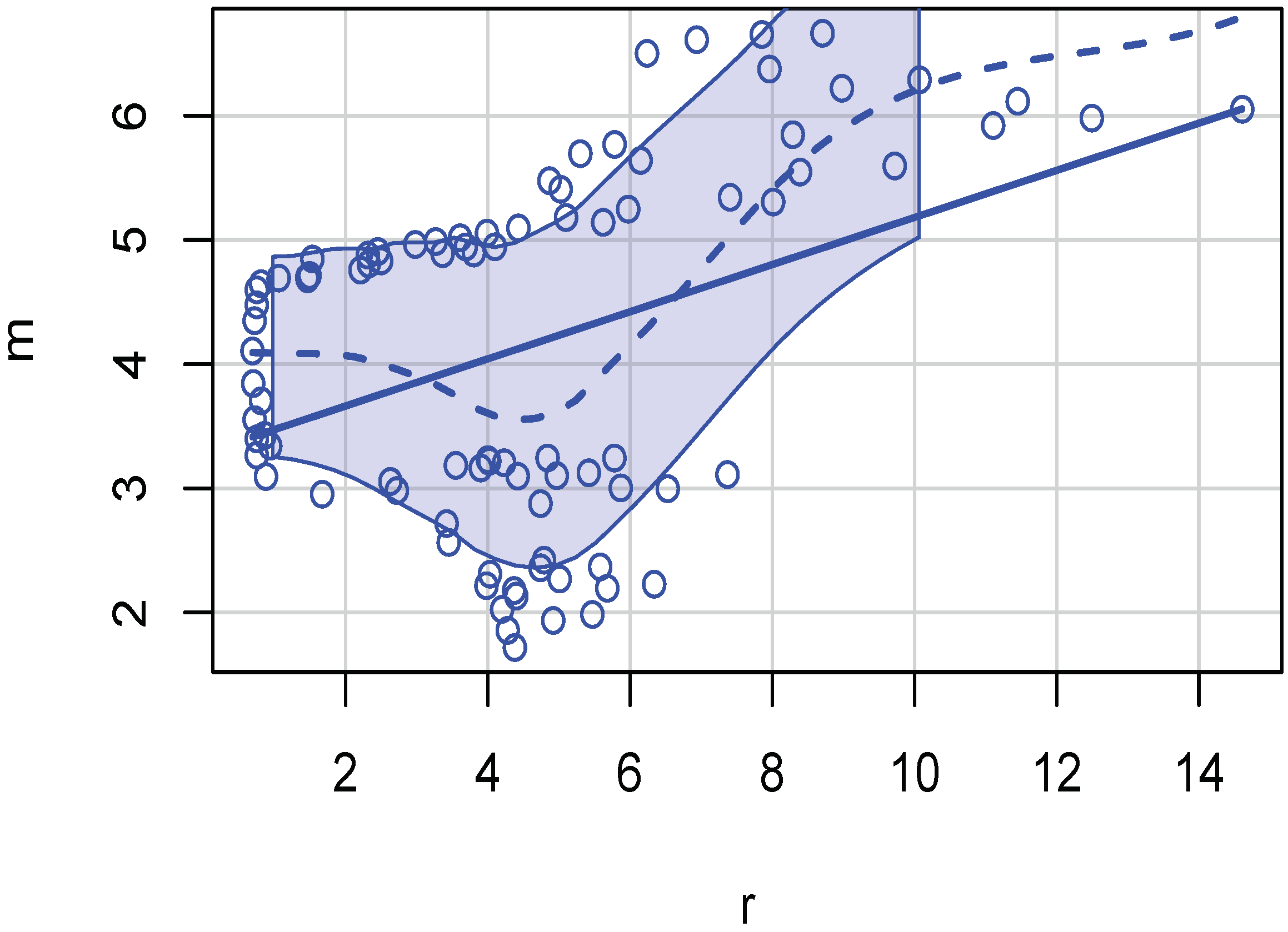
Now, we illustrate a scatterplot in Figure 2 showing that variables in the time-series data are not linearly related. The dashed lowess line (mentioned earlier in the context of Figure 1) is not straight. The evidence of nonlinearities implies a rejection of OLS.

Consider the potential endogeneity problem with the model specification where m depends on (p, y, r) after admitting nonlinear relations. As we did for the cross-section example, we use the causeSummBlk() algorithm of the R package ‘generalCorr’ to yield Table 4. This table is similar to Table 3, and the meaning of headings is described above in that context. See package vignettes for details regarding measuring the “strength” of causal dependence.

The plan of the remaining paper is as follows. Section 3 begins with Pearson’s symmetric correlation matrix $R=\left\{r_{ij}\right\}$ and its asymmetric generalization $R^{*}=\left\{r_{i|j}^{*}\right\}$, where $r_{i|j}^{*}\ne r_{j|i}^{*}$. Section 4 begins with defining usual partial correlation coefficients and develops generalized partial correlation coefficients (GPCC). Section 5 starts with a somewhat less well-known link between the usual partial correlations and scale-free standardized beta coefficients and generalizes it to GPCC. Section 6 describes proposed pseudo regression coefficients and includes our final remarks.

3. Generalized Measures of Correlation and ${\mathit{R}}^{*}$ Matrix

The product–moment (Pearson) correlation coefficient between variables $X_i$ and $X_j$ is:

$$r_{ij}=cov(X_i,X_j)/\surd (var\left(Xi\right)\ast var\left(X_j\right)).$$

(4)

It is helpful to view Pearson’s matrix of correlations, $R=\left\{r_{ij}\right\}$, in terms of flipped linear regressions among only two variables at a time, allowing us to extend them to kernel regressions in the sequel. Let us write the fitted values (denoted by hats) as conditional expectations for each pair of $X_i$ and $X_j$:

$$E\left(X_j\right|X_i)={\widehat{X}}_j^{OLS}.$$

(5)

Equation (5) provides a linear conditional expectation function ${\widehat{X}}_j^{OLS}\left(X_i\right)$ for each value of $X_i$. We also consider a flipped regression:

$$E\left(X_i\right|X_j)={\widehat{X}}_i^{OLS},$$

(6)

While OLS multiple correlations satisfy $R^2\left(X_i\right|X_j)=R^2\left(X_j\right|X_i)$, the kernel regressions do not. The product–moment correlation coefficient $r_{ij}$ of (4) is the square root of multiple correlations of flipped linear regressions.

The linearity assumption can underestimate the dependence by some 83% in a nonlinear example, where x has integers 1 to 10, and y = sin(x). Verify that $r_{yx}=-0.1705$ only, even though x and y are perfectly dependent (the absolute measure of dependence is unity). The R command generalCor::depMeas(y,x) yields $-1$ as the correct measure of dependence. Our Figure 1 and Figure 2 show that the cross-section and time-series models often present nonlinearities. Hence, our kernel regression software tools are better suited than OLS for a deeper understanding of dependence relationships.

Result 2

(Expression for $r_{ij}$ Ready for Generalized $R^{*}$ matrix). The elements of the usual correlation matrix R can be equivalently written as the signed square roots of multiple $R^2$ values of two flipped OLS regressions, illustrated by (5) and (6), as follows:

$$\begin{array}{c}\hfill r_{ij}=\mathrm{sign}\left(r_{ij}\right)\surd R^2\left(X_j\right|X_i)=\mathrm{sign}\left(r_{ij}\right)\surd R^2\left(X_j\right|X_i).\end{array}$$

(7)

Let the subscript t denote the observation number. A nonlinear, nonparametric kernel regression generalizes the OLS model as:

$$X_{jt}=G_j\left(X_{it}\right)+{ϵ}_{jt},t=1,\cdots ,T,$$

(8)

The flipped kernel regression obtained by interchanging $X_i$ and $X_j$ in Equation (8), is:

$$X_{it}=G_i\left(X_{jt}\right)+{ϵ}_{it},t=1,\cdots ,T.$$

(9)

The main attraction behind the kernel regressions is their superior fit to the data. It is accomplished by removing the requirement that a parametric formula should describe the regression relation.

Starting with the usual analysis of variance decomposition and assuming finite variances ($E{X}_i^2<\infty$ and $E{X}_j^2<\infty$), the generalized measures of correlation (GMC) defined by Zheng et al. (2012) are defined from the pair of flipped kernel regressions in (8) and (9). Assuming the respective fitted values are conditional expectations, ${\widehat{X}}_j=E\left(X_j\right|X_i)$ and ${\widehat{X}}_i=E\left(X_i\right|X_j)$, they define GMCs as variance ratios:

$$\begin{array}{cc}GMC\left(X_j\right|X_i)\hfill & =\left[\frac{var\left(E\left(X_j\right|X_i)\right)}{var\left(X_j\right)}\right]=\frac{ExplainedVariance}{TotalVariance},\hfill \\ GMC\left(X_i\right|X_j)\hfill & =\left[\frac{var\left(E\left(X_i\right|X_j)\right)}{var\left(X_i\right)}\right]=\frac{ExplainedVariance}{TotalVariance},\hfill \end{array}$$

(10)

computed as the multiple $R^2\left(X_j\right|X_i)$ and $R^2\left(X_i\right|X_j)$ from the two flipped kernel regressions. Since generalized measures of correlation (GMCs) are multiple $R^2$ from kernel regressions, we can recall Result 2 to generalize the OLS result of (7) by replacing OLS $R^2$ with GMCs as follows.

As measures of correlation, the non-negative GMC’s in the range [0, 1] provide no information regarding the up or down overall direction of the relation between $X_i$ and $X_j$, revealed by the sign of the Pearson coefficient $r_{ij}$. Since a proper generalization of $r_{ij}$ should not provide less information, Vinod (2017) proposes the following modification. A general asymmetric correlation coefficient from the $GMC\left(X_j\right|X_i)$ is:

$$r_{j|i}^{*}=\mathrm{sign}\left(r_{ij}\right)\surd GMC\left(X_j\right|X_i),$$

(11)

where $-1\le r_{j|i}^{*}\le 1$. It generalizes (7). A matrix of generalized correlation coefficients denoted by $R^{*}$ is asymmetric: $r_{i|j}^{*}\ne r_{j|i}^{*}$.

We are denoting generalized correlations by an asterisk. A function gmcmtx0(.), in the R package “generalCorr,” readily provides the $R^{*}=\left\{r_{X_i|X_j}^{*}\right\}=\left\{r_{i|j}^{*}\right\}$ matrix from a data matrix where $X_i$ denotes the row variable, and $X_j$ denotes the column variable. Note that the conditioning is always on the column variable, consistent with the matrix algebra convention of naming rows i and columns j.

4. Generalizing Partial Correlation and Standardized Beta Coefficients

The partial correlation $r_{12;3}$ equals the simple (linear) correlation between ($X_1,X_2$) after removing the effect of ($X_3$). A standard formula is:

$$r_{12;3}=\frac{r_{12}-r_{13}{r}_{23}}{\sqrt{(1-r_{13}^2)}\sqrt{(1-r_{23}^2)}}.$$

(12)

The numerator ($r_{12}-r_{13}{r}_{23}$) in (12) has the correlation coefficient between $X_1$ and $X_2$ after subtracting the linear effect of $X_3$ on them, while the denominator performs a normalization to obtain a scale-free correlation coefficient.

More generally, we start with p variables $X_i$, where $i=1,2,\dots p$. We want to consider the partial correlation coefficient between $X_i$ and $X_j$ after removing the effect of all remaining variables collectively denoted by $X_k$. A common derivation for the general case by Raveh (1985) uses the elements of the inverse matrix ${\left(R\right)}^{-1}$, which fails when ${\left(R\right)}^{-1}$ is unavailable. Our general correlation coefficient matrix $R^{*}$ is asymmetric, and its inverse is often unavailable. Hence, the next few paragraphs describe an equivalent but slightly cumbersome Kendall and Stuart (1977) method, which is always available for computing generalized partial correlation coefficients (GPCCs).

Consider the general case with p variables where OLS regression of $X_i$ on $X_k$ yields a residual vector denoted by $u_{i,k}$. Like $u_{i,k}$ above, $u_{j,k}$ is defined as the residual of the OLS regression of $X_j$ on all variable(s) $X_k$. Kendall and Stuart (1977) suggest that an alternate estimate of the usual partial correlation coefficient is the Pearson (symmetric) correlation coefficient between two relevant residuals as the partial correlation coefficient:

$$r_{ij;k}=U_{ij;k}=\frac{cov\left(u_{i,k}{u}_{j,k}\right)}{\sigma \left(u_{i,k}\right)\sigma \left(u_{j,k}\right)}.$$

(13)

Thus, one can compute the partial correlation coefficients for larger models with many regressors by using $X_k$ as a matrix of several variables and defining suitable residual vectors. Thus, one can always bypass Raveh’s formula requiring the existence of the inverse matrix $R^{-1}$.

5. Relation between Partial Correlations and Standardized Beta Coefficients

Recall that when $p=2$, estimates of standardized beta coefficients, denoted as $({\widehat{\beta }}_{12},{\widehat{\beta }}_{13})$, are obtained by regressing standardized $x_{1s}$ on $(x_{2s},x_{3s})$ in (2). Similarly, the standardized beta coefficients denoted as $({\widehat{\beta }}_{21},{\widehat{\beta }}_{23})$ are obtained by a similar regression (after interchanging 1 and 2, or flipped) of $x_{2s}$ on $(x_{1s},x_{3s})$. It is known that squared partials equal a product of flipped standardized beta coefficients:

$$r_{12.3}^2={\widehat{\beta }}_{12}{\widehat{\beta }}_{21}.$$

(14)

This equality may not be intuitively obvious, but is easily checked with the numerical values of an example.

A nonparametric kernel regression of $X_i$ on $X_k$ yields a residual vector denoted by $u_{i,k}^{*}$, with an asterisk added to distinguish it from OLS residuals $u_{i,k}$. While $u_{i,k}^{*}$ subtracts from $X_i$ nonlinear fitted values of $X_i$ based on $X_k$, analogous $u_{j,k}^{*}$ subtracts nonlinear fitted values of $X_j$ based on $X_k$. Now we are ready to define our GPCC based on $u_{i,k}^{*}$ and $u_{j,k}^{*}$, yielding a more general version of (13). Our GPCC uses the sign($U_{ij;k}^{*}$) similar to the sign appearing in (11). The GPCC also uses $R^2$ values (denoted as GMC’s) of flipped regressions identical to those used in defining the $R^{*}$ matrix in (11).

Now, the $R^2$ of kernel regression, $u_{i,k}^{*}=f\left(u_{j,k}^{*}\right)+{ϵ}_1$, is $GMC\left(u_{i,k}^{*}\right|u_{j,k}^{*})$. Similar $R^2$ of a flipped kernel regression, $u_{j,k}^{*}=f\left(u_{i,k}^{*}\right)+{ϵ}_2$, is $GMC\left(u_{j,k}^{*}\right|u_{i,k}^{*})$. The generalized partial correlations will be asymmetric since the $R^2$ of two flipped kernel regressions will be distinct, implying that

$$GMC\left(u_{i,k}^{*}\right|u_{j,k}^{*})\ne GMC\left(u_{j,k}^{*}\right|u_{i,k}^{*}).$$

Finally, we can define the asymmetric GPCC as:

$$r^{*}(X_i,X_j;X_k)=\mathrm{sign}\left({\mathrm{U}}_{\mathrm{ij};\mathrm{k}}^{*}\right)\surd \left[\mathrm{GMC}\left({\mathrm{u}}_{\mathrm{i},\mathrm{k}}^{*}\right|{\mathrm{u}}_{\mathrm{j},\mathrm{k}}^{*})\right].$$

(15)

Often, we simplify the notation and write the GPCC as $r_{i,j;k}^{*}$.

From elementary statistics, all correlation coefficients are pure numbers because they do not change if the variables are re-centered or rescaled (standardized). Accordingly, the GPCC of (15) is also a scale-free pure number. Furthermore, the scale-free GPCCs are non-symmetric quantities similar to standardized beta coefficients. After all, standardized beta coefficients of flipped regressions obtained by interchanging the subscripts i and j are rarely, if ever, identical.

Result 3

(GPCC are generalized standardized beta coefficients). Generalized partial correlation coefficients (GPCCs) are scale-free generalized standardized beta coefficients obtained by allowing for nonlinear relations.

Result 3 generalizes (14) or ($r_{12;3}^2={\widehat{\beta }}_{12}{\widehat{\beta }}_{21}$), where standardized betas are already asymmetric, leading to ($r_{12;3}^{*}{r}_{21;3}^{*}={\widehat{\beta }}_{12|3}^{*}{\widehat{\beta }}_{21|3}^{*}$). More generally, we use subscripts $(i,j,k)$ instead of (1, 2, 3) to write ${\widehat{\beta }}_{ij|k}^{*}=r_{ij;k}^{*}$. Thus, we accomplish the realism of asymmetry, ${\widehat{\beta }}_{12|3}^{*}\ne {\widehat{\beta }}_{21|3}^{*}$.

Hybrid GPCCs Are Useful When p Is Relatively Large

The definition (15) of GPCC attempts to remove the effect of all other variables $x_k$ on two main variables $x_i,x_j$. Its first term is the sign of $U_{ij;k}^{*}$ based on the covariance of residuals $u_{i,k}^{*}$ of kernel regression ${\widehat{x}}_i=E\left(x_i\right|x_k)$, and similar residuals $u_{j,k}^{*}$ of kernel regression ${\widehat{x}}_j=E\left(x_i\right|x_k)$. The sign is multiplied by the asymmetric generalized correlation coefficient $r^{*}$ between the two sets of residuals $u_{i,k}^{*}$ and $u_{j,k}^{*}$. Our GPCC $r_{ij;k}^{*}$ is the square root of the $R^2$ of the kernel regression of $u_{i,k}^{*}$ on $u_{j,k}^{*}$.

The kernel fitted values can be too close to the values of the dependent variable, leaving too little information in residuals. We fear that $u_{i,k}^{*}$ and $u_{j,k}^{*}$ may also have too little information, especially when there are several variables in $x_k$. Then, we suggest using a hybrid GPCC or HGPCC based on OLS residuals u. We call it hybrid because we use a nonparametric kernel regression (not OLS) to regress $u_{i,k}$ on $u_{j,k}$ (instead of $u_{i,k}^{*}$ and $u_{j,k}^{*}$ with the asterisk) in defining HGPCC as:

$$r^{h*}(X_i,X_j;X_k)=\mathrm{sign}\left({\mathrm{U}}_{\mathrm{ij};\mathrm{k}}\right)\surd \left[\mathrm{GMC}\left({\mathrm{u}}_{\mathrm{i},\mathrm{k}}\right|{\mathrm{u}}_{\mathrm{j},\mathrm{k}})\right],$$

(16)

where the two asterisks from the last GMC of Equation (15) are absent. One uses the square root of the $R^2$ of kernel regression of OLS residuals $u_{i,k}$ on $u_{j,k}$. Often, we simplify the notation and write the HGPCC as $r_{i,j;k}^{h*}$.

Our cross-section example of Section 2.1 has the following GPCCs, implying practical significance in a nonlinear setting: rounded to three places, $Sale=+0.004, RMC=-0.006,$ $OCost=0.035, PCost=0.087$, and $Lev=-0.144$. The practical significance in explaining ROA is lowest for the firm’s sales and highest for its leverage. These ranks are distinct from linearity-based results, even though leverage remains among the top two and sales remains among the bottom two in Table 1. Since the number of regressors here is small, the hybrid version is not recommended. We report HGPCC estimates for completeness as follows: $RMC=-0.0034,OCost=0.0056,sale=0.1531,PCost=-0.1648,Lev=-0.1734$.

Our macro time series example of Section 2.2 has the following GPCCs, $r=-0.125,$ $y=0.302,p=0.727.$ The GPCCs imply that the interest rates have the smallest and price level p has the highest practical significance in explaining money supply m in standard deviation units. This partly agrees with the linearity-based result that interest rates have the smallest practical significance in moving the money supply in standard deviation units in Table 2. Again, since the number of regressors in the model is small, one does not need the hybrid version. We report HGPCC’s practical significance estimates for completeness as follows: $r=-0.695,y=0.743,p=0.554$. The choice between GPCC and hybrid GPCC depends on the information contained in the relevant sets of residuals. We leave a deeper graphical analysis of two sets of residuals and a simulation for future work. Our current recommendation is to use GPCC, unless the number of regressors p exceeds 10.

6. Pseudo-Regression Coefficients and Final Remarks

The introduction to this paper lists three suggestions to avoid the p-hacking problem made by Wasserstein et al. (2019). More recently, Hirschauer et al. (2021) state that formal inference might often be “tricky or outright impossible” when it is not clear whether the observed data represent a random sample. This paper provides software tools to implement some of those suggestions while de-emphasizing p-values.

We argue for nonlinear, nonparametric kernel regressions to supplement the OLS. A wider acceptance of kernel regressions is hampered by the absence of something akin to regression coefficients. This paper suggests GPCCs and pseudo-regression coefficients as new tools to help practitioners compute the “practical significance” of regressors in addition to statistical significance.

The previous section defined the GPCC in (15) and a hybrid version HGPCC in (16). Result 3 has established that GPCCs are standardized (scale-free) regression coefficients for nonparametric kernel regressions. Ranking the absolute values of GPCCs helps to determine which regressor is the most important. Hence, GPCCs allow us to estimate the ‘practical significance’ of various regressors in explaining the dependent variable in standard deviation units. Starting with scale-free GPCCs, one can go back to the units in the original OLS specification of the model as follows.

We simply rescale the GPCCs similar to the rescaling of standardized beta coefficients in (3). The rescaling yields our new pseudo regression coefficients. If a kernel regression with the dependent variable y is specified as $y=G(X_i,i=1,\dots p)$, the pseudo regression coefficients are:

$$b_{yi}=r_{yi;k}^{*}\frac{sd\left(y\right)}{sd\left(X_i\right)},$$

(17)

where the standard deviations are based on all T observations. The computation of $r_{yi;k}^{*}$ is very simple by using parcorVec(.) from the R package ‘generalCorr,’ providing the vector of generalized partial correlation coefficients (GPCC). The pseudo-coefficients need not have any partial derivative interpretation.

Result 4

(Pseudo-Coefficients as Partial Derivatives). The pseudo-regression coefficients of kernel regressions can be considered partial derivatives of the dependent variable with respect to the relevant regressor.

An alternative to the “np” package used in the “generalCorr” package is the “NNS” package by Viole (2021). NNS offers a convenient function for computing the partial derivatives. Vinod and Viole (2018) report a simulation in their Section 4.1, where the NNS mean absolute percent error (MAPE) from the known true value of the derivatives is superior to the np package derivatives obtained by using the gradient option of a local linear fit by (regtype="ll"). Since nonparametric kernel regressions have no parametric coefficients, partial derivative estimates have been proposed as pseudo-regression coefficients in the literature. The cross-section example pseudo-coefficients given by the R command sudoCoefParcor() are RMC = −0.028, Lev = −0.185, Sale = 2.615, PCost = −0.503, and OCost = 0.101. The macro time series example has p = 1.309, y = 0.671, and r = −0.060 as the pseudo-coefficients based on GPCCs. Thus, this paper adds two new pseudo-regression coefficients based on GPCC and its hybrid version.

The usual partial correlation coefficients $r_{ij;k}$ are scale-free comparable pure numbers. Their absolute values can be sorted from the smallest to the largest to yield the order statistics, if needed. The regressor with the largest absolute partial correlation after removing the linear effect of all other variables in the regression is practically most significant. The GPCCs generalize these ideas so that the absolute values of scale-free $r_{ij;k}^{*}$ can be ordered from the smallest to the largest. They measure nonlinear practical importance in explaining standardized values of the dependent variable $X_i$. Regressors $X_j$ with a larger absolute GPCC with the dependent variable $|r_{ij;k}^{*}|$ suggest greater practical significance after incorporating nonlinearities.

This paper provides a cross-section and a time-series example.

The cross-section example illustrates how the evidence does not support hypothesis H1 in Khan et al. (2020) despite statistical significance cited by the authors. Thus, traditional t-tests need to be supplemented by newer tools.

The idea of comparing the practical contribution of each regressor by ranking the standardized beta coefficients is old, developed in the mid-20th century, but rarely used. What is new here is our nonlinear GPCC, $r_{yi;k}^{*}$, based on the generalized asymmetric correlation matrix, $R^{*}$. The R command parcorVec(mtx) yields GPCCs with the variable in the first column of the input matrix (mtx).

Our tools supplement statistical significance results. Our GPCCs reveal practical significance in nonlinear settings. Since practitioners need a way to compare the practical numerical impact of each regressor in a realistic nonlinear setting, the ideas discussed in this paper deserve further attention.

References

- Anderson, Torben J. 2008. The performance relationship of effective risk management: Exploring the firm-specific investment rationale. Long Range Planning 41: 155–76. [Google Scholar] [CrossRef]
- Anderson, T. J., and O. Roggi. 2012. Strategic Risk Management and Corporate Value Creation. Presented at the Strategic Management Society 32nd Annual International Conference, SMS 2012, Prague, Czech Republic; Available online: https://research-api.cbs.dk/ws/portalfiles/portal/58853215/Torben_Andersen.pdf (accessed on 10 January 2022).
- Brodeur, Abel, Nikolai Cook, and Anthony Heyes. 2020. Methods matter: p-hacking and publication bias in causal analysis in economics. American Economic Review 110: 3634–60. [Google Scholar] [CrossRef]
- Goodman, S. N. 2019. Why is Getting Rid of P-Values So Hard? Musings on Science and Statistics. The American Statistician 73: 26–30. [Google Scholar] [CrossRef] [Green Version]
- Hirschauer, Norbert, Sven Gruner, Oliver Mushoff, Claudia Becker, and Antje Jantsch. 2021. Inference using non-random samples? stop right there! Significance 18: 20–24. [Google Scholar] [CrossRef]
- Kendall, Maurice, and Alan Stuart. 1977. The Advanced Theory of Statistics, 4th ed. New York: Macmillan Publishing Co., vol. 1. [Google Scholar]
- Khan, Asad, Muhammad Ibrahim Khan, and Niaz Ahmed Bhutto. 2020. Reassessing the impact of risk management capabilities on firm value: A stakeholders perspective. Journal of Management and Business 6: 81–98. [Google Scholar] [CrossRef] [Green Version]
- Koopmans, Tjalling C. 1950. When Is an Equation System Complete for Statistical Purposes. Technical Report. Yale University. Available online: https://cowles.yale.edu/sites/default/files/files/pub/mon/m10-all.pdf (accessed on 10 January 2022).
- Mouras, F., and A. Badri. 2020. Survey of the Risk Management Methods, Techniques and Software Used Most Frequently in Occupational Health and Safety. International Journal of Safety and Security Engineering 10: 149–60. [Google Scholar] [CrossRef]
- Raveh, Adi. 1985. On the use of the inverse of the correlation matrix in multivariate data analysis. The American Statistician 39: 39–42. [Google Scholar]
- Valaskova, K., T. Kliestik, L. Svabova, and P. Adamko. 2018. Financial Risk Measurement and Prediction Modelling for Sustainable Development of Business Entities Using Regression Analysis. Sustainability 10: 2144. [Google Scholar] [CrossRef] [Green Version]
- Vinod, H. D. 2021a. Generalized, partial and canonical correlation coefficients. Computational Economics 59: 1–28. [Google Scholar] [CrossRef]
- Vinod, H. D. 2021b. generalCorr: Generalized Correlations and Initial Causal Path. R package Version 1.2.0, Has 6 Vignettes. New York: Fordham University. [Google Scholar]
- Vinod, Hrishikesh D. 2017. Generalized correlation and kernel causality with applications in development economics. Communications in Statistics—Simulation and Computation 46: 4513–34. [Google Scholar] [CrossRef]
- Vinod, Hrishikesh D., and Fred Viole. 2018. Nonparametric Regression Using Clusters. Computational Economics 52: 1317–34. [Google Scholar] [CrossRef]
- Viole, Fred. 2021. NNS: Nonlinear Nonparametric Statistics, R Package Version 0.8.3; Available online: https://cran.r-project.org/package=NNS (accessed on 10 January 2022).
- Wasserstein, Ronald L., Allen L. Schirm, and Nicole A. Lazar. 2019. Moving to a world beyond p less than 0.05. The American Statistician 73: 1–19. [Google Scholar] [CrossRef] [Green Version]
- Zheng, Shurong, Ning-Zhong Shi, and Zhengjun Zhang. 2012. Generalized measures of correlation for asymmetry, nonlinearity, and beyond. Journal of the American Statistical Association 107: 1239–52. [Google Scholar] [CrossRef]
Figure 1.
Cross-section example scatterplot of production cost and ROA illustrating presence of nonlinearity.
Figure 2.
Macro example scatterplot of m and r illustrating nonlinearity.