Dependence Structures between Sovereign Credit Default Swaps and Global Risk Factors in BRICS Countries

Abstract

This study investigates the tail dependence structures of sovereign credit default swaps (CDSs) and three global risk factors in BRICS countries using a copula approach, which is popular for capturing the “true” tail dependence based on the “distribution-adjusted” joint marginals. The empirical results show that global market risk sentiment comoves with sovereign CDS spreads across BRICS countries under extreme market events such as the pandemic-induced crash of 2020, with Brazil reporting the highest bilateral convergence followed by China, Russia, and South Africa. Furthermore, oil price volatility is the second biggest risk factor correlated with CDS spreads for Brazil and South Africa, while exchange rate risk exhibits very low co-dependence with CDS spreads during extreme market downturns. On the contrary, exchange rate risk is the second largest risk factor co-moving with China and Russia’s CDS spreads, while oil price volatility exhibits the lowest co-dependence with CDS in these countries. Between oil price and currency risk, evidence of single risk factor dominance is found for Russia, where exchange rate risk is largely dominant, and policymakers could promulgate financial sector regulations that mitigate spill-over risks such as targeted capital controls when markets are distressed.

1. Introduction

BRICS economies enjoyed a significant rise (i.e., quadrupled) in foreign investment inflows in the last 20 years as global investors diversify away risk and pursue investments with higher yields, resulting in net portfolio inflows peaking at USD 55.5bn in 2019, up from USD 12.3bn in 2009 (World Bank 2021). The continued deepening of bilateral and intergroup trade cooperation has ultimately resulted in inseparable interdependence across various macroeconomic fundamentals (see Figure 1 and Figure 2) such as external account balances, gross domestic product (GDP), portfolio investments, foreign (FX) liquidity reserves, interest rate spreads, foreign direct investment (FDI), and sovereign credit risk (CIA Factbook 2021). Among others, these fundamentals are key drivers of sovereign credit risk commonly measured by sovereign CDS spreads (Yang et al. 2018; Caillault and Guegan 2005; Wang et al. 2020; Blommestein et al. 2016; Tabak et al. 2016).

The first quarter (Q1) of 2020 witnessed a simultaneous and sudden spike in sovereign CDS spreads for all BRICS economies which coincided with the global oil price shocks and outbreak of the coronavirus pandemic, collectively amplifying negative global economic outlook and bearish market sentiments. The global pandemic outbreak resulted in severe socio-economic consequences such as an extended halt in cross-country tourism travel and shutdown in global trade activities, which further exacerbated the market volatilities and propagated large negative shockwaves, evident through the largest drops in global economic growth beyond the lowest lows recorded during the global financial crisis (GFC) (Wang et al. 2020). At this time, sovereign CDS spreads for all BRICS countries overshot to all-time highs (as much as 450 basis points for South Africa), exacerbated by noise traders executing knee-jerk reactionary trades ordering the mass disposal of emerging market bonds in their global portfolios. Investors hoarding their risky portfolios demanded a higher premium for holding emerging market risk, such as BRICS sovereign bonds, leading to an increase in the CDS spreads, which indicates the heightened cost of insuring against sovereign default risk. Therefore, understanding the dependence structure between CDS spreads and global risk becomes vital for financial stability.

From the BRICS perspective, the sovereign CDS literature is limited to examining CDS risk determinants and how driving factors compare between BRICS and G7 economies. A recent study on BRICS investigated the dependence structure of sovereign CDS and oil price volatility in BRICS and G7 countries using copula with wavelet analysis and found evidence of simultaneous co-movements during economic prosperity, but divergence was evident during macroeconomic downturns (Yang et al. 2018). They used copulas to investigate the intensity of association, which focused on the association of sovereign CDS spreads and exchange rate and/or oil price risk and reported the existence of empirical relationships across developed and emerging markets’ sovereign CDSs (Caillault and Guegan 2005; Wang et al. 2020).

While the above studies pioneered non-parametric analyses of sovereign CDSs and other global risks in the BRICS context, they focused on examining how global risks drive sovereign CDS volatility, with sovereign CDS presumed to be endogenously determined. These studies provide insights on how global risk factors influence sovereign credit risk; however, they are silent on whether the impact of such global determinants is linear and homogenous across BRICS. The cross- and within-country comparison of factor interdependence is presently ignored in the empirical literature. Against this backdrop and considering that sovereign CDS volatility is indeed a measure of sovereign credit risk, one can conjecture a possible dependency among global risk factors, especially during widespread market crashes such as the GFC where markets collapse jointly. A structurally heterogeneous block of countries such as BRICS could exhibit varying bivariate co-movement patterns, which must be considered by policymakers when formulating joint macroeconomic policies to advance the shared economic aspirations to compete in the global trade arena. To the best of our knowledge, very few existing studies have analysed the convergence between these risks, while most studies have attempted to use several risk factors to explain the uncertainty in sovereign credit risk. The imminent dependence structure between global risk factors remains unaddressed.

This study analyses the bivariate dependence structures between sovereign credit risk and individual global risk factors (oil price volatility, global sentiment, and exchange rate risks), with the underlying dependence structures assumed to differ within and across BRICS countries, due to idiosyncratic economic architectures such as the degree of exposure to import–export markets and structural strengths of the individual economies. The marginal propensity to consume global commodities such as oil could determine the impact intensity of oil price shocks such that heavy oil consumers get affected differently relative to light consumers that are self-sufficient net exporters. For example, heavy oil consumers such as China and Saudi Arabia are dependent on global oil supply dynamics to cover short-run domestic oil consumption demand; therefore, oil price fluctuations and exchange rate risks will materially alter procurement prices, while light oil consumers are unlikely to be heavily impacted (Galariotis et al. 2016).

Understanding the co-movement between global risk categories remains crucial to the global investors community and policymakers alike. Not only does risk dependence analysis help investors, asset managers, and portfolio analysts with risk-adjusted portfolio allocation decisions, but it also provides insights in setting and monitoring sectoral- or country-specific risk appetite. Given country-specific idiosyncrasies, regulators may equally gain insights on how global risks propagate into domestic financial markets and what their direct implications on a country’s risk perception are. This, in turn, may inform targeted policy interventions to mitigate the adverse effects of external risks on the domestic economy and local financial market. The next section reviews the existing literature and describes the methodology to fill the identified gap. Section 3 discusses the empirical findings, and the last section concludes.

2. Empirical Review, Materials and Methods

2.1. Empirical Literature Review

In the existing literature, dependence structure analysis is grounded on financial contagion or co-movement theory, which offers several reasons for convergence in financial returns and associated risk measures. Contagion theory describes the extreme propagation of financial shocks to other related markets, which manifests in various ways such as the spill-over of risks, co-movements, or the convergence of risks, herding behaviour, and coordinated aggregate demand shifts (Bauwens et al. 2012). The co-movement of risk factors arise as a manifestation of contagion, and this study focuses on bivariate co-movement as an implication of contagion risk, which is driven by growing the interconnectedness of the markets under study and their macroeconomic fundamentals (Yang et al. 2018; Ballester and González-Urteaga 2020; Boubaker and Sghaier 2013; Galariotis et al. 2016).

Based on this theory, financial returns converge in line with fundamentals as well as coordinated traders’ behaviour, causing sustained aggregate demand shifts in the financial markets, ultimately resulting in co-movements in fundamentally unrelated risk measures (Aas 2004). This theory predicts that, as aggregate demand in emerging market sovereign bonds gains bearish momentum during periods of elevated global risks, the sovereign CDS spreads ultimately rise (implying weakening credit risk profile), resulting in evident negative co-movements between sovereign CDSs and global risk sentiments (McNeil et al. 2002; Barberis et al. 2005). Similarly, stronger co-dependencies are predicted for CDSs and other global risks such as oil price risk and exchange rate risk.

The existing literature follows two distinct but related approaches in studying sovereign CDS and global risks factors; one assumes exogeneity, while the other approach relies on the endogeneity of CDS spreads. The first focuses on the contagion effects of CDS risks on the domestic market and macroeconomic fundamentals (Fermanian and Scaillet 2002; McNeil et al. 2002; Tabak et al. 2016). Accordingly, Grammatikos and Vermeulen (2012) reported the significant transmission of sovereign debt crisis shocks onto the European financial sector stock returns and exchange rates, a finding which is common in the literature (Wang et al. 2013; Ballester and González-Urteaga 2020). However, this approach is criticised for ignoring the indisputable impact of universal access to global financial markets, which is the conduit for colossal financial shockwaves in the debt capital markets (ultimately amplifying volatility in the domestic financial markets) during stressed macroeconomic conditions such as the global financial crisis (Blommestein et al. 2016; Brechmann 2010; McNeil et al. 2002; Tabak et al. 2016; Wang et al. 2020; Nelsen 2006).

The second approach considers sovereign CDS spreads as an endogenous factor and investigates the impact of various global risk factors on sovereign credit risk (Blommestein et al. 2016; Brechmann 2010). Global risk factors are exogenous in nature, and empirical evidence attests that the sovereign risk profile of emerging economies is demonstrably and evidently vulnerable to global shocks (Augustin et al. 2020; Tabak et al. 2016; Grammatikos and Vermeulen 2012). Therefore, the exogeneity assumption often fails empirical rigour, particularly in emerging markets where sovereign CDSs exhibit extreme volatility during periods of bearish global risk sentiment and catastrophic risk events such as a global financial crisis and the global coronavirus pandemic (Kalbaska and Gatkowski 2012; Alter and Beyer 2014; Augustin et al. 2020).

Recent empirical studies apply the theory of co-movements to investigate the relationship between risk factors, arguing that co-movements found in asset returns also occur across risk variables (Blommestein et al. 2016; Brechmann 2010; Tabak et al. 2016; Wang et al. 2013). Choe et al. (2020) recently examined systemic risk spill-overs in sovereign CDSs and focused on the contagion effect, reporting evidence of contagion risk and simultaneity during the European sovereign debt crisis and global financial crisis events. An Asian region-focused study documented evidence of co-movements in sovereign CDS spreads across Asian countries and major sub-regions, a result which is widely reported in the literature across developed and emerging markets (Alter and Beyer 2014; Fermanian and Scaillet 2002; McNeil et al. 2002; Tabak et al. 2016).

The study by Lovreta and Pascual (2020) analysed the dependence patterns between bank and sovereign credit risk using the endogenous estimation of the timing of structural breaks. The endogenous approach is superior to the exogenous selection of break dates commonly applied in the literature, and it prevents the problem of choosing the size and location of important turning points associated with extreme tail events. Their study reported three phases characterised by changes in the bank–sovereign dependence structure, and a bi-directional relationship was only evident at the peak of the European sovereign debt crisis.

Lovreta and Pascual (2020) also argued that endogenously detected turning points coincide with crucial public events that affect global investors’ risk perceptions on the government’s capacity and willingness to repay debt and support distressed banks. Their findings also evidenced that structural dependence in the system extends to co-movements between bank and sovereign credit risk volatility, as reported by Wang et al. (2020). While their study deployed a vector autoregressive (VAR) framework to study short-run dynamic linkages among financial markets, it is related to our work as it documents bivariate structural dependence between risk factors, which is the focus of our study. They used the VAR model a as benchmark and then analysed its stability using tests for structural changes of unknown, with results showing evidence of significant structural breaks on individual CDS returns series and on individual equations of the VAR system.

The latest study by Wang et al. (2020) used four Jump-GARCH models to forecast the jump diffusion volatility, which was used as the risk factor. The linear and asymmetric nonlinear effects were analysed, and the value at risk of banks was estimated by support vector quantile regression. They document three key findings. First, the Jump diffusion GARCH model is better than the Continuous Diffusion GARCH model, and the discrete jump volatility is significant in terms of the volatility process of bank stock price. Secondly, the jump behaviour of bank stock prices is heterogeneous due to different sensitivity to abnormal information shocks. Thirdly, the support vector quantile regression model performs better than the parametric quantile regression and nonparametric quantile regression for banks, based on the jump diffusion volatility information. Moreover, CJ-GARCH models are suitable for most banks, while ARJI-R2-GARCH models are more suitable for small- and medium-sized banks.

With various methodologies applied in the empirical literature, we note the contributions of Hasebe (2013) and Aas et al. (2009) in comparing the goodness of fits and inference for vine copulas when the bivariate copulas are all (i) t copulas, (ii) Gumbel copulas, (iii) Clayton copulas, and (iv) Frank/normal copulas (Aas and Berg 2009; Fischer et al. 2009). These bivariate copulas are either reflection symmetric or have one-directional (one of upper or lower) tail dependence. They used vine copulas with two-parameter bivariate linking copulas where lower tail dependence differed from upper tail dependence to check if there was some reflection asymmetry in the joint tails of financial asset returns. Their comparative results based on AIC and BIC show evidence that the Student-t copula is the optimally superior fit to capture tail dependences and reflective symmetry. The second-best copula fits were three families of bivariate copulas, namely BB1, BB4, and BB7 in the latter, which interpolate independence and the Frechet upper bound copulas and have upper and lower tail dependence that can range independently from 0 to 1. For robustness checks, they used five European market indices of similar sizes for analysis and comparison, and the conclusions were similar (Iuga and Mihalciuc 2020; Joe 1997).

This study builds upon the foundations laid by the extant literature and analyses co-movements across several risk factors such as sovereign credit risk and other global risk factors including oil price risk, risk sentiment, and exchange rate volatility. Within the BRICS context, the sovereign CDS literature is limited to examining how sovereign risk determinants compare between BRICS and developed economies, but bivariate risk factor co-dependence has received limited attention. The recent study by Yang et al. (2018) broadly examines core determinants of CDS risk and how risk factor intensity compares between BRICS and G7 economies, and their findings complement non-parametric studies based on copula techniques, which report co-movement between sovereign CDS spreads and exchange rate and/or oil price risk across developed and emerging markets. They investigated the dependence structure of sovereign CDS and oil price volatility in BRICS and G7 countries using copula with wavelet analysis and found evidence of simultaneous co-movements during economic prosperity, but divergence was evident during macroeconomic downturns (Yang et al. 2018).

The above studies pioneered the non-parametric analysis of sovereign CDS and other global risks in the BRICS context, investigating how global risks drive sovereign CDS volatility, with sovereign CDS presumed to be endogenously determined. While they explain how global risk factors influence sovereign credit risk for BRICS economies, they are silent on whether the impact of such global drivers is homogenous within and across BRICS countries if one considers that BRICS countries are structurally diverse in their political and economic architecture. During extreme market downturns such as financial crashes (Global pandemic-market crash of 2020), the emerging markets’ credit fundamentals and risk indicators collapsed alongside each other concurrently, suggesting that risk factors could be correlated and converge overtime, as documented in stylised facts in the literature (Aas and Berg 2009; Grammatikos and Vermeulen 2012). Where bivariate co-dependence exists, the nature of bilateral convergence could be too costly to ignore for a block of heterogeneous countries, which can exhibit varying bivariate interaction patterns.

This study seeks to provide cross- and within-country comparison of the dependence structures between individual global risk factors and sovereign CDS spreads in BRICS. The rest of this study is structured as follows: Section 2.2 presents the data and methodology, Section 3 discusses the empirical results, while Section 4 concludes the study with some policy implications.

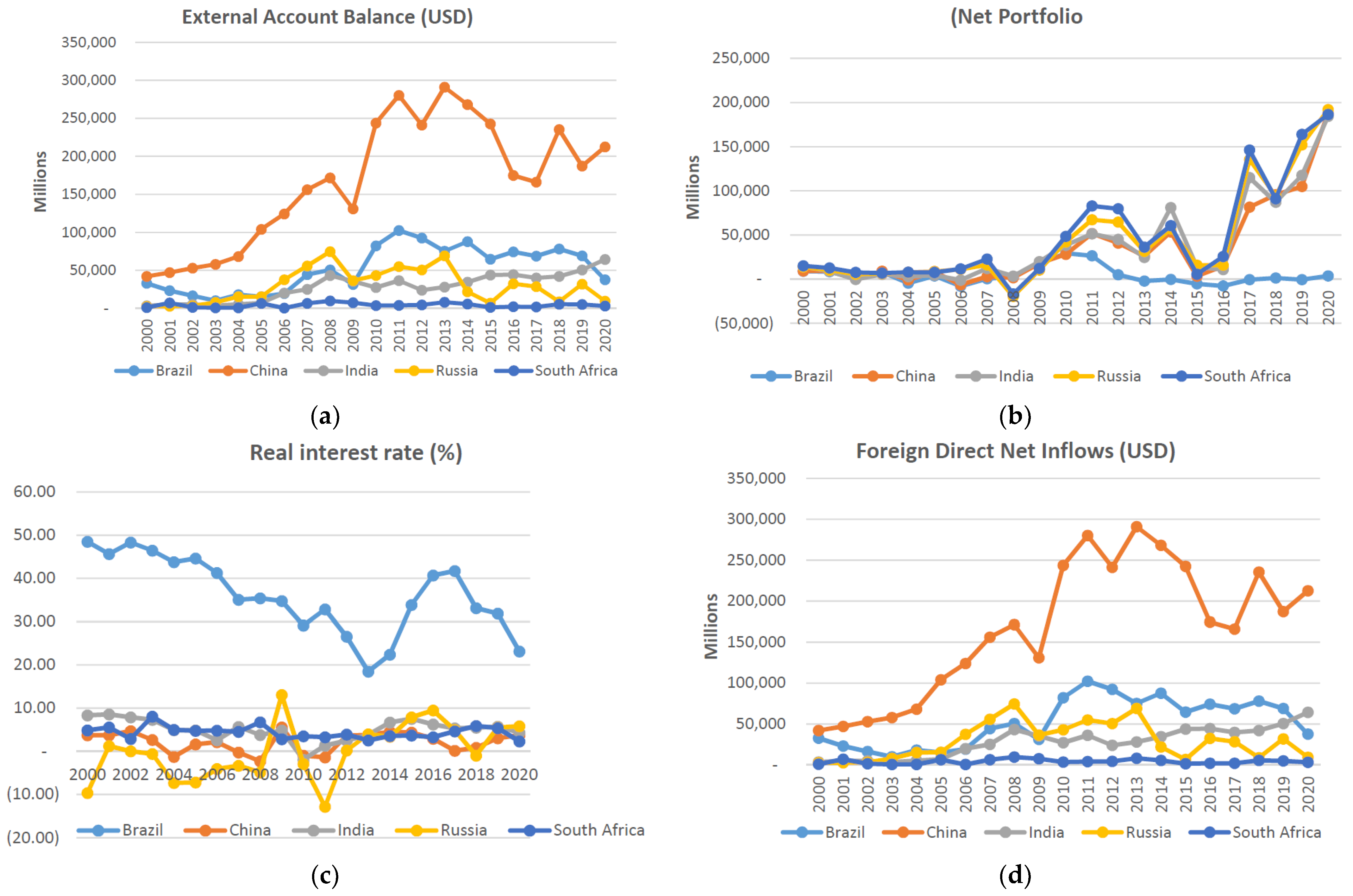
2.2. Data Description, Transformations, and Visual Inspections

2.2.1. Data Scoping, Collection Frequency, and Transformations

This empirical study used daily observations sourced from Thomson Reuters of the Brent crude oil price, global equity market volatility index, local exchange rates against the US dollar, and sovereign CDS spreads data collected over five years from 21 March 2016 to 18 March 2021. The sovereign CDS spreads and exchange rates for Brazil, Russia, China, and South Africa were collected for further analysis, but India was excluded due to the limited availability of data on sovereign CDS spreads. Most importantly, the scope of analysis was aligned to the maturity profile of the sovereign CDS contracts (up to five years’ maturity), which represents the highly liquid and most actively traded sovereign CDSs in the secondary market, thereby allowing for the collection of high-frequency data or daily observations for all variables. On the contrary, if one selects 10 years’ maturity CDS contracts, high-frequency data are limited due poor liquidity on longer–dated instruments compared to 5 year CDSs that are highly traded, supported by sufficient depths of short-dated tenor instruments (Lovreta and Pascual 2020; Wang et al. 2020; Yang et al. 2018).This scope is consistent with many leading papers that examined the dependence structure of sovereign CDSs and other risk factors across many developed and developing markets (Wang et al. 2020; Kalbaska and Gatkowski 2012; Alter and Beyer 2014).

All data collected was converted into daily returns which are stationary, with the augmented Dickey–Fuller (ADF) tests confirming the absence of unit roots. The daily returns were calculated using the natural logarithm of today’s closing price divided by the closing price of the previous day, formally represented by the below function:

$$r_t=ln\left(\frac{P_t}{P_{t-1}}\right)=ln\left(\frac{{Index}_t}{{Index}_{t-1}}\right)$$

(1)

where $P_t$ is the daily closing price of Brent crude oil, exchange rate, and sovereign CDS spread, while ${Index}_t$ is the closing level of global equity market volatility, and $r_t$ represents the daily logarithmic changes in each variable collated for further descriptive analysis, and the results are summarised in Table 1.

The daily changes in sovereign CDS spreads are used as a proxy for sovereign credit risk, implying that huge spikes in sovereign CDS spreads are indicative of the increased riskiness of sovereign assets, as CDS providers demand higher risk premia (or high spreads) to compensate for perceived incremental default risks on the underlying sovereign credit obligations to the investors (Hansen and Lunde 2005; Joe 1996). Global market risk sentiment is extracted from daily changes in the global equity market volatility index. Furthermore, daily changes in exchange rates and Brent crude oil price are collated and used as inputs to extract the daily volatility of oil price and exchange rates against the US dollar by fitting appropriate generalised autoregressive conditional heteroskedasticity (GARCH) processes.

The daily volatilities extracted from GARCH models are used as the daily observations of exchange rate risk and oil price risk over the five years, while sovereign CDS and global risk sentiment are analysed using daily returns, not daily volatility. Before fitting the GARCH process to model volatility, we fitted a standard autoregressive moving average with one lag (i.e., ARMA (1,1)) as a mean model and GARCH (1,1) with one lag as a variance model as GARCH process specification. Hansen and Lunde (2005) analysed model performance and proved that the GARCH (1,1) model outperforms complex model specifications in the modelling of volatility using high-frequency data such as daily and intra-day returns; therefore, our study draws support from this finding, upon which we deploy the GARCH (1,1) model to model daily volatility in this study. In finance studies, GARCH (1,1) is a popular choice to filter the error series with Student-t distribution with a variance of 1 (Jondeau and Rockinger 2006; Joe 1997; Nelsen 2006).

To extract the daily volatility, we fitted the ARMA (1,1)–GARCH (1,1) model with standard and exponential error distributions to determine if there are symmetrical effects of previous volatility on present-day observations and plotted the QQ plot and News Impact Curve for further visual inspection before conducting goodness of fit tests. The fitted ARMA (1,1) GARCH (1,1) model is defined below:

$$r_t={\alpha }_0+\varphi r_{t-1}+\theta {\epsilon }_{t-1}+{\epsilon }_t$$

(2)

$${\sigma }_t^2={\alpha }_0+{\alpha }_1{\epsilon }_{t-1}^2+\beta {\sigma }_{t-1}^2+{\mathsf{{\rm Y}}}_1{I}_{t-1}{\epsilon }_{t-1}^2$$

(3)

where:

$$I_{t-1}=\{\begin{array}{ll}1& if {\epsilon }_{t-1}<0\\ 0& if {\epsilon }_{t-1}\ge 0.\end{array}$$

where the $r_t$ is the mean model and ${\sigma }_t^2$ is the estimated variance of the empirical data, which is represented by the residuals from fitted GARCH models. The variance series represents daily volatility in the exchange rates and oil price, which is the measure of oil price risk and currency risk for this study.

GARCH models belong to a family of parametric estimation techniques; therefore, they require a particular distribution to be imposed, such that in this study, a standard GARCH (sGARCH) and exponential GARCH (eGARCH) both have standard and exponential distributions, respectively. That said, the GARCH process is the most popular in the empirical literature for modelling volatility in the financial time series (Lovreta and Pascual 2020; Nelsen 2006). The sGARCH model imposes a non-negative parameter constraint, which is an overly restrictive assumption and presumes that negative shocks have the same effect as positive innovations, and this presumption is generally not supported by financial returns data. However, the eGARCH model overcomes the non-negativity parameter constraints in the linear model, as there are no restrictions in the exponential function, which is equipped to handle negative values (Lovreta and Pascual 2020; Aas et al. 2009).

While due care was taken to ensure appropriate innovations distribution was assigned during the preliminary data analysis, an exponential GARCH(1,1) model was the best-fitted model to extract daily volatility because it captures the leverage effect of volatility persistence, to reflect that positive/negative shocks do not have the same impact, but the prior assumption of empirical error distribution remains a limiting factor compromising the effectiveness of the GARCH(1,1) model. However, this is not overly concerning, as the extracted volatility series is time invariant and used as input into the bivariate VineCopula process, which considers the autoregressive nature of volatility. While Copulas are non-parametric techniques used to analyse tail dependence, they are unable to capture time-varying dependence structures. That said, Copulas deployed are time invariant, while volatility can be time varying, and this is noted as a methodological limitation to be explored in future studies on this subject.

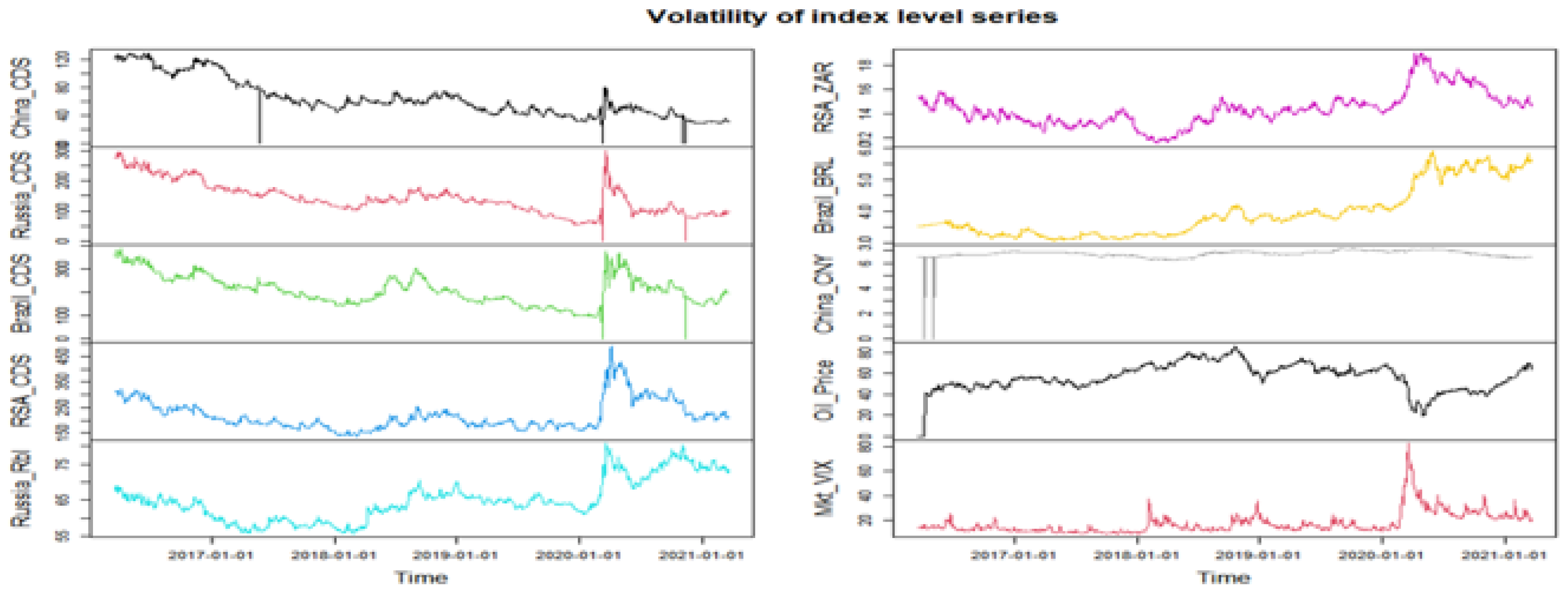
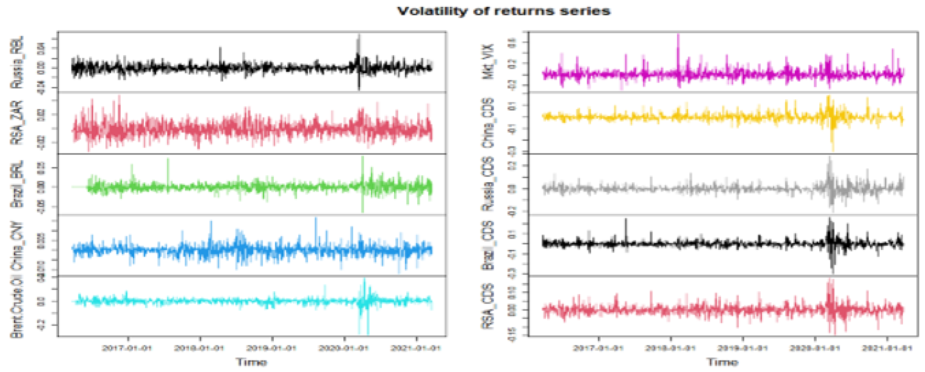
2.2.2. Visual Inspection of Daily Volatilities and Changes in CDS and Global Risks

For this study, changes in sovereign CDS spreads were used as proxy for sovereign credit risk profile, implying that huge spikes in sovereign CDS spreads implies the increased riskiness of sovereign assets, as CDS providers demand higher-risk premia (or high spreads) to compensate for perceived incremental default risks on the sovereign credit obligations held by investors. Global market risk sentiment is observed from changes in the global volatility index, as represented by logarithmic changes in the Chicago Board of Exchange equity volatility index (VIX). Furthermore, the logarithmic changes in the exchange rates and oil price were used as inputs to extract daily volatility by fitting appropriate generalised autoregressive conditional heteroskedasticity (GARCH) processes to extract daily volatility for Brent crude oil prices and each local currency against the US dollar.

Volatility clusters appear around the same time in the return’s series, and notably large volatility clustering prevailed in Q1 2020 when massive global oil price shocks occurred, signifying that sovereign CDS spreads spiked to record highs during the oil price shock events, and changes in global risk sentiment also peaked to the highest levels when global oil prices plummeted to record lows (see Figure 2 and Figure 3). Volatility is modelled using GARCH processes which consider the time-varying and autocorrelated nature of residuals series over time, which are attributes characterising exchange rate and oil price history (see visual presentations and GARCH tests). Accordingly, the GARCH process was used to extract daily volatility (variance), and copulas were used to assess the underlying dependence structures and compare that against linear correlation coefficients, which presupposes that empirical financial data follow elliptical distributions.

Figure 1. Macroeconomic variables. (a) external account balance; (b) Net portfolio investment inflows—bonds; (c) Interest rate spreads; (d) foreign direct investment inflows (USA’bn).

Figure 1. Macroeconomic variables. (a) external account balance; (b) Net portfolio investment inflows—bonds; (c) Interest rate spreads; (d) foreign direct investment inflows (USA’bn).

Figure 2. Overview of BRICS sovereign CDS spreads, oil price, exchange rate and global volatility (VIX).

Figure 2. Overview of BRICS sovereign CDS spreads, oil price, exchange rate and global volatility (VIX).

Figure 3. Volatility of returns series, reflecting recursive volatility clusters.

Figure 3. Volatility of returns series, reflecting recursive volatility clusters.

The GARCH models extracted daily volatility for oil price and exchange rates which was used for further analysis of dependence structure, with results summarised in Table 2 and Table 3. Key observations from the fitted GARCH models exhibit strong evidence of the asymmetric impact of historical shocks on the present-day volatility of oil prices and exchange rates, with the empirical results confirming that the exponential (eGARCH) term is statistically significant in modelling exchange rates and Brent crude oil price risks. Hence, this evidence indicates that positive historical oil price shocks have higher effects than negative shocks on the present-day volatility, which means the impact is asymmetrical (Longin and Solnik 2001).

2.3. The Optimal Copula

The correlated movements of financial variables are widely studied in the empirical literature, with many studies often analysing dependence structures using simple correlation and other linear measures, which hinge on the assumption of normal distribution (Aas 2004). However, the normality of financial returns data lacks empirical rigour; therefore, any statistical inference drawn remains questionable (Ballester and González-Urteaga 2020; Brechmann 2010). Against this backdrop, several non-parametric techniques have been developed and utilised in the recent literature, and copulas have gained strong research utility in financial econometrics (Blum et al. 2002). The study by Lokshin and Sajaia (2004) deployed maximum likelihood estimation (MLE) techniques to estimate a bivariate sample-selection model and the endogenous switching regression model, respectively, under the assumption of the joint normality of marginals. However, the resultant estimators are biased and inconsistent if joint normality assumption is used, which is often violated by empirical financial returns exuding thicker tails than normal distribution implies. To overcome this shortcoming, the copula approach is useful both to relax the assumption of prior normality and estimate the models using maximum likelihood techniques so that the estimators attain adequate efficiency (Hasebe 2013).

A copula C can be defined as a function linking univariate marginal distributions to the joint multivariate distribution functions of at least two random variables and the permit further decomposition of any n-dimensional joint distribution into its marginals, thereby allowing for the accurate description of joint distributions without relying on the assumption of distributional normality (Aas 2004). Copula theory gains more popularity among researchers for the capability to simultaneously extract dependence structures from the joint probability distribution function and isolate such dependence structures from univariate marginals (Boubaker and Sghaier 2013). Copulas overcome the restrictive assumption of joint normality in financial time series and are often used in empirical research (Bouye et al. 2000; Embrechts et al. 2001, 2003; Aas and Berg 2009).

Formally, we define Copula C as an n-dimensional random vector $x=\left(x_1, x_2\right)$ for two dimensions (n = 2), with joint distribution function $F=\left(x_1, x_2\right)$ and marginal distributions $F_i\left(x_i\right)$ where the subscript $i=1, 2$. Given this construct, Sklar’s theorem states that there exists a copula $C\left(u_1, u_2\right)$ such that:

$$\left(x_1, x_2\right)=P\left(X_1<x_1, X_2<x_2\right)=C\left(F_1\left(x_1\right), F_2\left(x_2\right)\right)$$

(4)

If $F_i$ are continuous, then the copula $C\left(u_1, u_2\right)$ is unique. Copulas permit different degrees of tail dependence, the upper and the lower tail dependence, which are expressed formally as follows:

$${\lambda }_U=\underset{U\to 1^{-}}{\lim }P\left(U_1>u|U_2>u\right)=\underset{U\to 1^{-}}{\lim }\frac{C^{*}\left(u, u\right)}{1-u}$$

(5)

$${\lambda }_L=\underset{U\to 0^{+}}{\lim }P\left(U_1<u|U_2<u\right)=\underset{U\to 0^{+}}{\lim }\frac{C\left(u, u\right)}{u}$$

(6)

where $C^{*}$ is referred to as the survival copula.

Therefore, a copula can be interpreted as a function linking the marginal distributions of a random vector to its joint distribution (Aas 2004; Aas and Berg 2009). Many types of dependence structures exist to estimate joint marginal distributions, but for simplicity, we present five dependence structures from the Archimedean family, which are found to be more common in this empirical study—see Section 3.3.1.

The approach adopted in this study was to use the VineCopula package to identify the best-fitting and most optimal copula family type for each bivariate pairs of risk factors and sovereign CDSs. The benefit of using the VineCopula package is that is automated and streamlined the process to detect the most optimal copula family that best fit the data under study (Akaike 1973). Furthermore, the authors did not have to fit and run multiple separate copula tests and manually compare the AIC/BIC parameters to detect the best-fitted copula model, which is an operational inefficiency noted in the approach used by recent studies and leading papers in this subject (Hasebe 2013). We ran VineCopula model selection to obtain the optimal bivariate copula type for daily returns and volatility series as inputs and produce the most optimal copula family based on the AIC and/or BIC criteria after adjusting for the necessary penalties for estimating parameters. The copulas fitted for this study were variants that that all fell under the Archimedean and elliptical copulas defined below. In general, most bivariate pairs were best-fitted using the Student-t copula, which is consistent with other studies (Yang et al. 2018; Aas and Berg 2009). The VineCopula model selection brought efficiency to the model selection process by automating the comparison of information criterion and significantly reduced the time taken by researchers to compare goodness of fit measures, which is the process followed in the existing literature (Heinen and Valdesogo 2009; Fischer et al. 2009; Nelsen 2006). This model selection approach not only compared the information criterion but also imputed necessary penalties for parameter estimations, which is often overlooked when comparing model fits based on AIC/BIC (Hasebe 2013; Lokshin and Sajaia 2004; Min and Czado 2010).

2.3.1. Optimal Copulas Using VineCopula Package

The daily residuals for oil price and exchange rate and changes in global volatility (VIX) were merged with the sovereign CDS spread changes and used as inputs into the bivariate VineCopula process to best select the most optimal copula family type for each bivariate pair of sovereign CDS and each global risk. The optimal copula types were deduced from the VineCopula package and then fitted into the empirical data for further analysis of tail dependence structures and to estimate co-dependency parameters for each bivariate sovereign CDS and risk factor combination. Vine copulas are gaining popularity in empirical finance studies for their pair-copula construction capabilities and the fact that they account for reflection asymmetry when financial returns data exude varying lower or upper tail dependence parameters for each bivariate marginals (Schirmacher and Schirmacher 2008; Aas et al. 2009; Aas and Berg 2009; Heinen and Valdesogo 2009; Fischer et al. 2009; Min and Czado 2010). When d-dimensional vine copulas are sufficiently specified, vine copulas can account for flexible dependence structures through the specification of d, and all bivariate marginals of the vine copula have upper/lower tail dependence if the bivariate copulas at level 1 have upper/lower tail dependence structures. Vine copulas include multivariate normal and Student-t copulas as special cases (Joe et al. 2010; Schirmacher and Schirmacher 2008; Min and Czado 2010).

The bivariate model specification has two equations: a selection equation and an outcome equation, which are defined as follows:

$$S_t^{*}=\{\begin{array}{ll}0,& if S_t^{*}=z_t^{~} \gamma +{\epsilon }_{si}\le 0\\ 1,& if S_t^{*}=z_t^{~} \gamma +{\epsilon }_{si}>0\end{array}$$

(7)

where $S_i$ is an indicator of selection and $z_i$ is a vector of covariates, and the outcome of interest is observable when $S_i=1$, such that

$$y_i=\{\begin{array}{cc}{x}_t^{~} \beta +{\epsilon }_{1i}& if S_i=1\hfill \\ 0& if S_i=0\hfill \end{array}$$

(8)

If the errors, ${\epsilon }_{si}$ and ${\epsilon }_{1i}$ in the above equations are not independent, the ordinary least-squares (OLS) regression estimates of β are biased and inconsistent.

According to Aas (2004), the best-fitting copula type is given by minimising the distance of empirical copula of the data, where empirical copula ($C_e$) is given by:

$$C_e\left(u_1, u_d\right)=\frac{1}{n}{\sum }_{1=1}^n{\prod }_{j=1}^{d}I ({{\displaystyle \cup }}_{i,j}<u_j)$$

(9)

and the optimal minimisation function is defined by:

$$distance \left(C, C_e\right)=\sqrt{{\displaystyle \sum _{i=1}^n\sum _{d=1}^n}{(C(\frac{i_1}{n},,,,\frac{i_2}{n})-C_e(\frac{i_1}{n},,,, \frac{i_2}{n}))}^2}$$

(10)

The VineCopula packages solve this optimisation problem defined by Equation (8), and the ultimate optimal copula family is chosen using the Akaike and Bayesian Information Criteria (AIC and BIC, respectively), with the selection criteria formally defined and represented below:

For observations $u \left(i, j\right), i=1,\dots \dots \dots \dots \dots ,N, j=1,\dots \dots \dots \dots ,N$, the AIC of a bivariate copula family $C^N$ with parameter(s) $\left\{\mathit{\theta }\right\}$ is defined as:

$$AIC=-2{\displaystyle \sum }\left\{i=1^N|\ln [c\left(u \left(i, 1\right), u \left(i, 2\right)|\mathit{\theta }\right]+2k\right\}$$

(11)

where $k=1$ for one parameter copulas and $k=2$ for the two parameters copula.

Similarly, the BIC is obtained by:

$$BIC=-2{\displaystyle \sum }\left\{i=1^N|\ln [c\left(u \left(i, 1\right), u \left(i, 2\right)|\mathit{\theta }\right]+ln\left(N\right)k\right\}$$

(12)

Firstly, all available copulas are fitted using maximum likelihood estimation. Then, the criteria are computed for all available copula families and the family with the minimum value is chosen. Evidently, if the BIC is chosen, the penalty for two-parameter families is stronger than when using the AIC. Copulas are not nested relative to each other; therefore, the above information criterion are useful to identify the best copula family (Aas and Berg 2009; Heinen and Valdesogo 2009). If the marginals are fixed and the parameters to be estimated are the same, a copula with the smallest information criterion has the largest log-likelihood value, and therefore, will be identified as the most optimal copula for that bivariate pair of sovereign CDS and risk factors, as demonstrated by Hasebe (2013).

2.3.2. Pairwise Tail-Dependence of Sovereign CDS and Global Risks

Considering the overwhelming statistical evidence showing that distributional normality assumption does not hold for BRICS, as affirmed by J-B goodness of fit tests, we avoided drawing statistical inference based on measures of association assuming normality such as Spearman linear correlation coefficient. Therefore, this study deployed the copula approach, which consistently gains research popularity to measure dependence structure, as copulas can identify the true underlying distributional properties of an empirical data set (Blum et al. 2002; Aas et al. 2009). Copulas are appealing in modelling financial returns because of their strong capability to examine skewness and kurtosis to detect the underlying distribution of empirical data (Bouye et al. 2000).

In this study, we used copulas to investigate tail dependence structures, which allowed for the extrapolation of co-movements in sovereign CDS and global risks when extreme market volatility or tail events occur. Optimal copulas are fitted to each bivariate empirical combination to extract tail dependence structures, with results summarised in Table 3 under Section 3.3.1 of the results discussion. Below, we formally present Archimedean and elliptical copulas relevant to this study. Gaussian and Frank types are elliptical copulas, while Clayton and Gumbel are asymmetrical and exhibit greater tail dependence on the upper and lower tail ends of the distribution, capturing asymmetries.

Gaussian Copula

Gaussian copula is symmetrical with negative and positive tail dependence netting each other off to zero, which is formally defined as follows:

$$C_{\rho }\left(u_1, u_2\right)={\int }_{-\infty }^{{\varphi }_{u_1}^{-1} \left(u_1\right)}{\int }_{-\infty }^{{\varphi }_{u_1}^{-1} \left(u_2\right)}\frac{1}{2\pi }\frac{1}{\sqrt{1-{\rho }^2}} exp\left\{-\frac{x^2-2\rho xy+y^2}{2\left(1-{\rho }^2\right)}\right\} dxdy$$

(13)

where $\rho$ is the copula parameter and ${\varphi }^{-1}(.)$ represents the inverse of the standard univariate normal distribution function with a mean of zero and variance of one.

The coefficients of the upper and lower tail dependence are given by:

$${\lambda }_{\mathbb{L}} \left(\mathsf{{\rm X}},\mathsf{{\rm Y}}\right)={\lambda }_{\mathbb{U}} \left(\mathsf{{\rm X}},\mathsf{{\rm Y}}\right)=2\underset{x\to \infty }{\lim } \varphi \left(1+\frac{\sqrt{1-\rho }}{\sqrt{1+\rho }}\right)=0$$

(14)

Due to symmetry, twice the sum of positive and negative tail events equals zero for Gaussian copulas. This means that even if the correlation is very high, the extreme tail events occur independently, and the variables do not exhibit co-movements over time (Aas 2004).

Frank Copula

A Frank copula is symmetrical and behaves like a Gaussian copula by netting off positive and negative tail dependence to zero, which is formally defined as follows:

$$C_F\left(u_1, u_2\right)=-\frac{1}{\theta }ln\left(1+\frac{\left(e^{\theta u_1}-1\right)\left(e^{\theta u_2}-1\right)}{e^{-\theta }-1}\right)$$

(15)

The generator is given by:

$$\varphi \left(t\right)=-ln\left(\frac{e^{-\theta t}-1}{e^{-e}-1}\right), \mathrm{where}\theta \ne 1$$

(16)

Both the positive and negative dependence are equal to zero because they are symmetrical. In this instance, a stronger linear correlation does not imply tail dependence. If tail events are observed, then the extreme observations occur independently of each other (Aas 2004).

Student-t Copula

A Student-t copula, unlike the Gaussian and Frank types, can account for joint fat tails in the distribution function and an increased probability of joint extreme events, which makes it superior to the Gaussian or the elliptical copula family, in general. With smaller degrees of freedom, Student-t distribution can exhibit thicker tails than the other two distributions (Manner 2007). Formally, a Student-t copula is defined as follows.

$$C_{\rho , \upsilon }\left(u_1, u_2\right)={\int }_{-\infty }^{t_{u_1}^{-1} \left(u_1\right)}{\int }_{-\infty }^{t_{u_1}^{-1} \left(u_2\right)}\frac{1}{2\pi }\frac{1}{\sqrt{1-{\rho }^2}} \left\{1+\frac{x^2-2\rho xy+y^2}{\upsilon \left(1-{\rho }^2\right)}\right\} ds dt$$

(17)

where $\rho$ and $\upsilon$ are parameters of the Student-t copula and $t_v^{-1}$ is the inverse of the standard univariate Student-t distribution with $\upsilon$ degrees of freedom, the statistical mean of zero and variance defined by $\frac{\upsilon }{\upsilon -2}$. A Student-t copula has a degrees of freedom $\upsilon$ parameter, such that, when $\upsilon$ increases, the tendency of extreme co-dependency decreases. The dependence coefficients of upper and lower tails are given by:

$${\lambda }_{\mathbb{L}} \left(\mathsf{{\rm X}},\mathsf{{\rm Y}}\right)={\lambda }_{\mathbb{U}} \left(\mathsf{{\rm X}},\mathsf{{\rm Y}}\right)=2 t_{v+1}\varphi \left(\sqrt{1+\rho } (\frac{\sqrt{1-\rho }}{\sqrt{1+\rho }})\right)$$

(18)

whereby $t_{v+1}$ is the distribution function of a univariate Student-t distribution with $\upsilon +1$ degrees of freedom. For higher linear correlation $\rho$, the degrees of freedom $\upsilon$ will be smaller, and the tail dependence will be stronger. Most importantly, a Student-t copula denotes asymptotic tail dependence when linear correlation coefficient $\rho$ is negative and/or zero.

Clayton Copula

This is an asymmetric Archimedean and exhibits greater dependence on the negative tails than it does in the positive tails. It is formally expressed by:

$$C_c\left(u_1, u_2\right)=\max \left[{\left(u_1^{-\theta }+u_2^{-\theta }-1\right)}^{-{\theta }^{-1}}, 0\right]$$

(19)

and the generator is given by:

$$\varphi \left(t\right)={\theta }^{-1}\left(t^{-\theta }-1\right), \mathrm{where}\theta ϵ[-1,+\infty [\backslash \{0\}$$

(20)

The positive (upper tail, $U_C$) and negative (lower tail, $L_C$) tail dependence are given by:

$${\lambda }_{u_c}=0 \mathrm{and}{\lambda }_{L_c}$$

(21)

A Clayton copula captures co-dependency for extreme lower tail events and accounts for asymmetry which the Student-t copula does not allow due to restrictive parameters under the Student-t copula.

Gumbel Copula

This is also an asymmetric Archimedean but is different from Clayton in that it exhibits a greater dependence in the upper tail than the lower tail. It is formally expressed by:

$$C_G\left(u_1, u_2\right)=exp\left(-{\left[-ln{\left(u_i\right)}^{\theta }+{\left(-ln\left(u_2\right)\right)}^{\theta }\right]}^{{\theta }^{-1}}\right)$$

(22)

The generator is given by the following:

$$\varphi \left(t\right)={\left(-ln\left(t\right)\right)}^{\theta }, \mathrm{where}\theta \ge 1$$

(23)

The positive (upper tail, $U_G$) and negative (lower tail, $L_G$) tail dependence are given by:

$${\lambda }_{U_G}=2-2^{-\theta } \mathrm{and}{\lambda }_{L_G}=0$$

(24)

The Gumbel copula captures co-dependency for extreme higher tail events and accounts for asymmetry which Student-t copula does not accommodate, due to the restrictive parameters thereon.

3. Results Discussion and Interpretation

3.1. Exploratory Analysis of Daily Returns Structure

Table 1. Descriptive statistics.

Descriptive Statistics: First Difference of Each Variable							Volatility: Oil Price and Currency
Parameter Estimate	dRSA_CDS	dRussia_CDS	dChina_CDS	dBrazil_CDS	dVIX	dCrude_Oil	CHN_Yuan	BRA_Real	RSA_Zar	RUS_Rbl
Mean	0.000	−0.001	−0.001	−0.001	0.0	0.000	0.00	0.00	0.00	0.00
Min	−0.148	−0.208	−0.297	−0.299	−0.30	−0.28	−0.012	−0.065	−0.03	−0.05
Max	0.186	0.283	0.190	0.267	0.768	0.191	0.017	0.800	0.049	0.070
Std. Dev (%)	2.842	3.423	3.187	3.502	8.490	2.612	-	-	-	-
Kurtosis	6.000	10.830	10.820	17.220	8.860	24.83	3.690	6.980	1.010	7.320
Skewness	0.620	0.890	0.330	1.140	1.560	−1.47	0.330	0.580	0.390	0.890
J–B Stat	2049 ***	6570 ***	6409 ***	16,441 ***	4808 ***	34,065 ***	766 ***	2696 ***	88 ***	3094 ***
ADF Test	−23.78	−25.171	−24.959	−23.328	−28.1	−24.376	-	-	-	-
Cor_dCrude Oil	0.001	−0.015	−0.029	0.055	0.069	1.0	−0.003	−0.069	−0.03	−0.01
Cor_dMkt_VIX	0.297	0.225	0.096	0.378	1.0	0.069	0.009	0.000	−0.01	−0.02

Source: Own calculations using Thomson Reuters data. *** Statistically significant results at 1% level.

Table 1. Descriptive statistics.

Descriptive Statistics: First Difference of Each Variable							Volatility: Oil Price and Currency
Parameter Estimate	dRSA_CDS	dRussia_CDS	dChina_CDS	dBrazil_CDS	dVIX	dCrude_Oil	CHN_Yuan	BRA_Real	RSA_Zar	RUS_Rbl
Mean	0.000	−0.001	−0.001	−0.001	0.0	0.000	0.00	0.00	0.00	0.00
Min	−0.148	−0.208	−0.297	−0.299	−0.30	−0.28	−0.012	−0.065	−0.03	−0.05
Max	0.186	0.283	0.190	0.267	0.768	0.191	0.017	0.800	0.049	0.070
Std. Dev (%)	2.842	3.423	3.187	3.502	8.490	2.612	-	-	-	-
Kurtosis	6.000	10.830	10.820	17.220	8.860	24.83	3.690	6.980	1.010	7.320
Skewness	0.620	0.890	0.330	1.140	1.560	−1.47	0.330	0.580	0.390	0.890
J–B Stat	2049 ***	6570 ***	6409 ***	16,441 ***	4808 ***	34,065 ***	766 ***	2696 ***	88 ***	3094 ***
ADF Test	−23.78	−25.171	−24.959	−23.328	−28.1	−24.376	-	-	-	-
Cor_dCrude Oil	0.001	−0.015	−0.029	0.055	0.069	1.0	−0.003	−0.069	−0.03	−0.01
Cor_dMkt_VIX	0.297	0.225	0.096	0.378	1.0	0.069	0.009	0.000	−0.01	−0.02

Source: Own calculations using Thomson Reuters data. *** Statistically significant results at 1% level.

Skewness and kurtosis are crucial measures that determine whether the empirical data are normally distributed or non-normal, which is important to ascertain before analysing correlation measures which presuppose that underlying data are normally distributed. Skewness measures whether the distribution of data is symmetrical or asymmetrical, which is the overarching quality of normally distributed random variables. The values for skewness between −0.5 and +0.5 are considered acceptable to prove normal univariate distribution, while skewness greater than +1 or less than −1 depicts highly skewed empirical data (Aas 2004; Hair et al. 2017, p. 61). Kurtosis measures whether the distribution of empirical data is too peaked or too flat, and kurtosis below −1 indicates too flat distribution, while kurtosis greater than +1 indicates highly peaked distributions, implying that such heavily peaked or too flat distributions are not normal (Hair et al. 2017, p. 61). Kurtosis and skewness measured outside the above guidelines represent empirical data that are not normally distributed, and Jarque–Bera (J-B) goodness of fit tests are useful to determine if the kurtosis and skewness fit within normal distribution parameters.

The changes in sovereign CDSs for South Africa, Russia, and China are symmetrical, while Brazil is heavily skewed to the right, which implies that tail risk events occur independently for the former countries, while there is a positive tail dependence structure for Brazil. Changes in global risk sentiment and crude oil price are heavily skewed, signifying that tail events are dominant, and the data may not be normally distributed. Again, this implies that empirical tail observations are likely to exemplify asymmetric and positive tail dependence structure for this bivariate pair (Heinen and Valdesogo 2009; Hong and Preston 2005). The kurtosis measure is greater than +1 for all variables, which is evidence of heavily peaked distribution that violates the properties of normal distribution. The kurtosis and asymmetry measures for BRICS and global risk factors are not consistent with normal distribution properties. This means that tail observations are prevalent in the empirical financial data; therefore, correlation measures assuming symmetry will result in inaccurate relationship inferences (Aas and Berg 2009; Heinen and Valdesogo 2009).

The J-B goodness of fit test is conducted to conclusively determine if the empirical data are normally distributed. The J-B test statistics are positive, and it is close to zero for normally distributed data. That is, the further away it is from zero, the stronger the evidence that empirical data are not normally distributed. The J-B test statistic is extremely high, and the p-value is 0.00, thus reaffirming that BRICS data are not normally distributed.

Considering this evidence, it is not appropriate to analyse the dependency structure of sovereign CDSs and global risk factors using measures of association that assume distributional normality such as Spearman correlation coefficient. Hence, we need to analyse the dependency structure considering the underlying distributional properties of each variable and their combined marginal distributions, and this outcome is best achieved by using copulas to simultaneously decompose univariate dependence structures and link the marginals to the joint distributions without prior assumption on the univariate distribution. In this study, we analysed the association between and contrasts of the dependence structures of sovereign CDSs and global risk factors using both Spearman correlation coefficient and rank dependent measures on “distribution-corrected data” obtained from copulas and show that copula-based results are more robust and reliable than simple Spearman correlation measures.

As shown in Table 1, changes in sovereign CDS spreads were broadly negative and almost negligible on average terms; however, focusing on average changes overlooks the inherently persistent volatility in the spreads, as evidenced by massive variance between the day’s minimum and maximum intraday spreads. To this end, the standard deviation provides a more accurate indication of the realised volatility, which ranges from 2.84% to 3.5% for the group understudy, with Brazil recording the highest volatility of 3.5%, while South African had the lowest at 2.84%.

The standard deviation of oil prices and sovereign CDS spreads is much higher in the 2020–2021 period, possibly because of several shocks that occurred including the global oil price shocks in 2020 and the deterioration in global market sentiment due to the coronavirus outbreak, among others risks, resulting in abrupt adverse changes (i.e., deterioration) in the sovereign credit risk profile of emerging markets. The standard deviation of global risk sentiment was the highest at 8.5%, and oil price changes averaged 2.6%. The augmented Dickey–Fuller (ADF Test) confirms stationarity at first difference at the 0.1% significance level, which satisfies the necessary and required conditions to apply GARCH processes to model volatility of the exchange rates and oil price series.

3.2. Linear Dependence Structures—Simple Linear Correlation Measure

Table 2. Linear correlation of sovereign CDSs and risk factors.

Linear Dependence: Spearman Correlation for Sovereign CDS Spreads and Risk Factors
Daily Log Changes			Daily Volatility of Oil Price and Exchange Rate
	dVIX	dCrude_Oil	Crude_Oil	CHN_Yuan	BRA_Real	RSA_Zar	RUS_Rbl
dRSA_CDS	0.297	0.001	0.004	-	-	−0.018	-
dRussia_CDS	0.225	−0.015	−0.012	-	-	-	0.154
dChina_CDS	0.096	−0.029	−0.027	0.026	-	-	-
dBrazil_CDS	0.378	0.055	0.058		−0.042	-	-
Corr_dCrudeOil	0.069	1.0	1	−0.003	−0.069	−0.033	−0.058
Corr_dMkt_VIX	1.0	0.069	0.069	0.009	0.000	−0.010	−0.330

Source: Own calculations using data from Thomson Reuters.

Table 2. Linear correlation of sovereign CDSs and risk factors.

Linear Dependence: Spearman Correlation for Sovereign CDS Spreads and Risk Factors
Daily Log Changes			Daily Volatility of Oil Price and Exchange Rate
	dVIX	dCrude_Oil	Crude_Oil	CHN_Yuan	BRA_Real	RSA_Zar	RUS_Rbl
dRSA_CDS	0.297	0.001	0.004	-	-	−0.018	-
dRussia_CDS	0.225	−0.015	−0.012	-	-	-	0.154
dChina_CDS	0.096	−0.029	−0.027	0.026	-	-	-
dBrazil_CDS	0.378	0.055	0.058		−0.042	-	-
Corr_dCrudeOil	0.069	1.0	1	−0.003	−0.069	−0.033	−0.058
Corr_dMkt_VIX	1.0	0.069	0.069	0.009	0.000	−0.010	−0.330

Source: Own calculations using data from Thomson Reuters.

The Spearman correlation between crude oil price risk and sovereign CDS spreads differs across countries, showing very weak and negligible positive association for South Africa (0.4%), while Brazil has the highest correlation of 5.8%, which reflects the high exposure to global oil price movements as a net exporter of oil. Similarly, oil price risk exerts negative influence on Russian and Chinese sovereign CDS spreads, with China’s credit risk being the most negatively impacted compared to Russia’s credit risk profile. Similarly, the correlation between sovereign CDS and global risk sentiment is positive across all countries under review but strong and more pronounced for Brazil (38%) and South Africa (30%), while it is the weakest for China (10%). This means that positive global markets news is associated with noticeable improvement in credit risk spreads for BRICS sovereign bonds, and the opposite is true for deterioration in global market risk sentiment. This observation is consistent with studies reporting similar results for BRICS countries which are crucial emerging markets that are integral to global economic architecture.

Most importantly, changes in global risk sentiment affect sovereign credit risk more than oil price risk for BRICS economies, which is exacerbated by temporary but colossal portfolio outflows fuelled by knee-jerk, large-scale disposals of higher-yield emerging markets sovereign bonds and migrating funds into haven investment instruments such as US treasury bills during the period of heightened uncertainty. The correlation strength between exchange rate risk and sovereign CDS is generally weak across countries but is negative for South Africa and Brazil, while it is positive for China and Russia. Although it is relatively weak, Russia’s sovereign CDSs depict a relatively stronger association with currency volatility than all countries across BRICS, while South Africa’s sovereign CDSs are the least affected by currency volatility.

3.3. Analysis of Empirical Results: Tail Dependence Structures for BRICS Countries

3.3.1. Pairwise Tail Dependence of Risk Factors and Sovereign CDS

This section breaks down the dependency structure between sovereign CDSs and a suite of global risk factors based on Vine copulas, which are used to decompose implicit dependence structures from empirical data. Copulas are used to assess dependence structures to overcome the overly restrictive assumption of normality in the distribution of marginals, which compromises the legitimacy and accuracy of inferences drawn based on simple Spearman correlation measurements. Given the violation of distributional normally (J-B normality test with p-values of 0.00), this study used the VineCopula package to determine the underlying marginals and identify the optimal copula type that fit each bivariate combination of sovereign CDS and global risk factors, without making assumptions of prior marginals. The best-fit copula type was chosen based on the AIC criteria and then fitted onto the bivariate combinations to extract the true rank dependent measure of association, with the results summarised in Table 3 below for further discussion on the next section.

Table 3. Dependency structure of sovereign CDS and global risk factors in BRICS.

Parameter Estimate	Oil Price Volatility		Global Markets Sentiment (dVIX)		Exchange Rate Volatility
Dependency Type	Spearman	Copula	Spearman	Copula	Spearman	Copula
Brazilian CDS	0.058	0.093	0.378	0.347	−0.042	−0.047
Copula_family	-	surJoe	-	surBB1/Gumbel	-	Student-t
Chinese CDS	−0.027	−0.028	0.096	0.314	0.026	0.038
Copula_family	-	Student-t	-	TawnT1	-	Student-t
Russian CDS	−0.012	−0.004	0.225	0.268	0.154	0.165
Copula_family	-	Student-t	-	surBB7/Clayton	-	Student-t
South African CDS	0.004	0.009	0.297	0.258	−0.018	0.006
Copula_family	-	Student-t	-	surBB1	-	Student-t

Source: Own calculations using data from Thomson Reuters.

Table 3. Dependency structure of sovereign CDS and global risk factors in BRICS.

Parameter Estimate	Oil Price Volatility		Global Markets Sentiment (dVIX)		Exchange Rate Volatility
Dependency Type	Spearman	Copula	Spearman	Copula	Spearman	Copula
Brazilian CDS	0.058	0.093	0.378	0.347	−0.042	−0.047
Copula_family	-	surJoe	-	surBB1/Gumbel	-	Student-t
Chinese CDS	−0.027	−0.028	0.096	0.314	0.026	0.038
Copula_family	-	Student-t	-	TawnT1	-	Student-t
Russian CDS	−0.012	−0.004	0.225	0.268	0.154	0.165
Copula_family	-	Student-t	-	surBB7/Clayton	-	Student-t
South African CDS	0.004	0.009	0.297	0.258	−0.018	0.006
Copula_family	-	Student-t	-	surBB1	-	Student-t

Source: Own calculations using data from Thomson Reuters.

The direction of association estimated by optimal copulas and linear correlation measure is consistent, both confirming positive or negative co-movements of bivariate combinations, as Student-t copula is the most common and it exhibits elliptical properties while accounting for tail dependence. The reason for this is that the Student-t copula caters for extreme negative values, thereby capturing varying lower/upper tail dependence structures, as lower tail dependence can be larger than upper tail dependence or vice versa. Empirically, asymmetric tail dependence is more commonly reported in the literature during more extreme market downturns or financial crashes (Jondeau et al. 2007; Nikoloulopoulos et al. 2010; Giacomini et al. 2009; Longin and Solnik 2001; Ang and Chen 2002).

The strength of a copula’s dependency structure is more robust and accurate, as it incorporates the empirical marginal distribution of each variable in the bivariate copula process, thereby overcoming the restrictive presumption of normal distribution of marginals under the Spearman correlation measures. However, South African (RSA) CDS spreads and exchange rate risk present an exceptional case where the dependency structure changes from negative (Spearman) to positive under distribution-corrected, copula-based measure but remains fairly negligible. This finding further reinforces the assertion that when the presumed joint normality of marginals is violated empirically, dependence measures and relationship inferences drawn are likely inaccurate and spurious at best, as widely documented in the existing literature (Nikoloulopoulos et al. 2010; Hasebe 2013; Nelsen 2006; Joe 1997). Although the magnitude is low, the copula-based dependence structure is positive between RSA CDS and exchange rates.

Furthermore, the most valuable exposition from bivariate copulas is the reaffirmation of the J-B normality test, confirming that the underlying empirical marginal distributions are not normal for all variables. However, there is sufficient evidence of symmetry between exchange rate volatility and sovereign CDSs across all BRICS countries, as confirmed by Student-t copula fitment as the most optimal copula type to model the empirical data. From an empirical perspective, the most optimal copula type is the Student-t copula for oil price risk and sovereign CDSs, signifying the existence of reflection symmetry of oil volatility on sovereign credit risk for China, Russia, and South Africa. Student–t copulas capture reflective symmetry while sufficiently differentiating between upper and lower tail dependence between bivariate covariates, and this finding is aligned to existing empirical results documented in several studies (Brechmann 2010; Joe 1997; Choe et al. 2020; Lovreta and Pascual 2020; Hansen and Lunde 2005). They applied alternative mixture copula models to account for asymmetrical tail dependence, which our study captured through the Student-t copula as the most optimal copula family. Our results show that the dependency strength reduces (whether positive or negative under Spearman measure) to lower strength under a copula measure but remains very small, except for Brazil, where there was an increase from 5.8% to 9.3% under the empirical marginal distribution-adjusted measures.

Brazil presents a unique case where the optimal copula type is the survival Joe copula, which captures asymmetrical tail dependence effects arising from extreme negative tail observations, signifying those negative extreme events have a greater association with Brazilian sovereign credit risk. The negative dependence reflects the structural design of Brazil’s economy, which benefits a lot from advanced industries producing and processing oil for final consumption, such as petroleum processing, automotive, cement, iron, and chemical production industries. In 2020, Brazil’s daily oil production averaged 3.78 mn barrels per day (bpd), making it the eighth largest global oil producer with a 4% global market share (World Bank 2021). That said, this tail dependence structure signifies that Brazil’s sovereign CDS spreads are negatively associated with an extreme drop in global oil prices, while extreme oil price gains do not materially move the sovereign CDS spreads. This result is expected, as Brazil earns foreign exchange profits and fiscal revenues from oil exports which, if they plummet significantly, could adversely impact fiscal revenues. Conversely, extreme price gains do not have extreme benefits, as the gains are shared with the largest producers such as the United States of America and Saudi Arabia.

What differentiates Brazil’s dependence structure from peer oil producers such as China and Russia (production at 4.86 mn bpd with 5% market share and 10.5 mn bpd with 11% market share, respectively) is their disproportionate share and varying propensity to consume large oil quantities in their domestic economies. That is, China and Russia consume 14.1 mn bpd and 3.7 mn bpd, with a global consumption market share of 14% and 4%, respectively. Therefore, the domestic economies in China and Russia consume very large quantities of oil production, while Brazil consumes very little relative to their production, resulting in larger exports to the global markets. As a net-exporter of oil, the size of exports and expected oil revenues are vulnerable to shocks induced by global oil supply dynamics and exchange rate volatility in the emerging markets. Therefore, the country’s marginal propensity to consume oil could also determine the resultant dependence structure amongst oil producers in BRICS.

Our empirical results confirmed that optimal copula family for sovereign CDSs and exchange rate volatility is Student-t copula across all countries, reflecting symmetry which is largely documented in the existing literature. The Student-t copula is appropriate and consistent for the underlying bivariate data (refer to skewness and kurtosis in Table 1), which reflects symmetric dependence structure, reinforcing the empirical findings in other geographies (Longin and Solnik 2001; Ang and Chen 2002; Hong and Preston 2005). For the global risk sentiment, the optimal copulas are the survival type (Joe–Clayton/Gumbel) or Tawn type copulas, which are asymmetrical and consider tail observations, and this variable exhibits the strongest (and most positive) association with sovereign CDS spreads of BRICS than any other global risk factor under consideration in this study. An increase in global risk sentiment causes an increase in sovereign CDS spreads, which implies a deterioration in perceived credit quality as global investors take bearish market views. This implies that global risk sentiment co-moves with sovereign CDSs when extreme tail-end observations occur, such that negative sentiment weakens CDSs, while extreme market optimism improves CDS spreads for sovereign issuers and banks (Wang et al. 2020). Our results are balanced enough to highlight that Vine copulas can yield different optimal bivariate copula pairs, depending on the market structure. Caillault and Guegan (2005) reported the naïve estimation of tail dependence parameters, showing symmetric bivariate dependence structures for the Thailand/Malaysian markets and asymmetric for the Thailand/Indonesian markets and for the Malaysian /Indonesian markets.

3.3.2. Comparison of Tail Dependence Structures within and across BRICS Countries

There is overwhelming empirical evidence that global market sentiment is a crucial positive driver of sovereign CDS spreads in BRICS. Brazil has the highest positive correlation (38%) followed by China (31%), Russia (27%), and South Africa (26%), implying that Brazil’s sovereign CDSs are more vulnerable to global risk sentiment, while South Africa is the least impacted across BRICS. This positive dependency is expected for emerging markets economies that are generally characterised by higher-yield sovereign bonds and liberalised financial markets which offer international investors seamless access to local financial markets to facilitate portfolio investments and foreign direct investment flows. Therefore, these countries must consider financial sector regulations that mitigate major risks that accompany the globalisation of access to local financial markets to proactively manage the impact on the country’s credit risk profile, which ultimately affects costs of borrowing and fiscal debt service costs.

Furthermore, oil price risk is the second biggest driver of sovereign CDS spreads for Brazil (9.3%) and South Africa (0.9%), while exchange rate risk exhibits a very small contribution to changes in sovereign CDS spreads. On the contrary, exchange rate risk is the second-largest influential factor for China (3.8%) and Russia’s (16.5%) sovereign CDS spreads, while oil price volatility contributes the lowest: 2.8% and 0.4%, respectively. The massive cross-country variation is largely driven by different exchange rate regimes adopted by each respective country (e.g., China operates under a pegged currency system, while other economies are on flexible exchange rate regimes), and China’s position as the largest oil consumer in the world plays a sizable role. Russia’s exposure to oil price volatility is the least significant factor to sovereign CDS spreads, as oil price hedging positions alleviate potential oil revenue volatility from currency fluctuations, and its position as a net importer provides benefits from prepaid orders.

The dependency structure of CDS/exchange rate risk and CDS/oil price volatility also differ significantly within each country, where one risk factor largely dominates at a massive scale, such as Russia, where exchange rate risk scores a dependence of 16.5%, which is highly dominant compared to oil price risk, with a dependence of −0.4%. Similar observations hold for Brazil, where the CDS/oil price volatility strength stands at 9.3% compared to a CDS/currency risk correlation strength of 4.7%. Finally, China exhibits a CDS/currency volatility dependence of 3.8% compared to the CDS association to oil price risk of −2.8%. This finding is very crucial for Russia to consider in financial sector policy formulation, where it is important to introduce policy measures to mitigate the large impact of currency volatility on the fiscal oil revenues, given that an increase in currency risk leads to an increase in sovereign CDS spreads. The oil price risk remains well contained through existing hedging arrangements, ultimately resulting in negligible impact on CDS spreads.

Brazil and China’s cases are slightly different; the scale dominance effect is very moderate compared to Russia, implying that Brazil and China cannot exclusively regulate or proactively manage spill-overs from one risk factor to mitigate overall spill-over risks on sovereign CDS spreads, and ultimately the sovereign credit risk profile. On the contrary, the South African dependency structure is unique; empirical evidence suggests global risk sentiment (26%) is the single largest driver of sovereign credit risk, while exchange rate risk and oil price volatility have negligible dependence with the sovereign CDS spreads.

4. Conclusions

This study examined the tail dependence structure of sovereign credit risk and each of three selected global risk factors for the BRICS community using the copulas approach, which is known for its ability to provide the “true” tail correlation based on the correct marginal distribution. The empirical results show that global market risk sentiment is very crucial in driving sovereign CDS spreads in the BRICS countries under extreme market events, with Brazil having the highest co-dependency, followed by China, Russia, and South Africa. This dependency is expected for emerging markets that are generally characterised by higher-yield sovereign bonds and internationally liberalised financial markets which offer foreign institutional investors seamless access to local markets to facilitate portfolio investments and foreign direct investment flows. Therefore, it is critical for BRICS policymakers to consider financial sector regulations that mitigate spill-over risks, such as capital controls under distressed markets, to maintain financial system stability, which can arise from unrestricted access to local financial markets by risk-averse foreign investors. Such a policy can proactively manage the impact of global sentiment on a country’s credit risk, which ultimately affects borrowing capacity and fiscal debt service costs.

Furthermore, oil price volatility is the second biggest risk factor correlated with sovereign CDS spreads for Brazil and South Africa, while exchange rate risk exhibits very small co-movements to changes in sovereign CDS spreads, under extreme market conditions dominated by tail events. On the contrary, exchange rate risk is the second largest risk factor associated with China and Russia’s sovereign CDS spreads, while oil price volatility exhibits the lowest association to CDS in these countries. Between oil price and currency risk, evidence of single risk factor dominance is found for Russia, where exchange rate risk is largely dominant (second to global sentiment), implying that Russia can mitigate or manage spill-over effects on sovereign CDS spreads by enacting financial sector regulations that mitigate exchange rate risk.

The optimal copula family for sovereign CDSs and exchange rate volatility is confirmed as the Student-t copula across all countries, suggesting symmetry, and this is consistent with expectations documented in the existing literature. For the global risk sentiment, the optimal copula is the survival type (Joe–Clayton/Gumbel) of Tawn type copulas which are asymmetrical and reflect one-sided tail dependence, and this variable has the strongest (and most positive) association with sovereign CDS spreads of BRICS than any other global risk factor studied. This implies that global risk sentiment co-moves with sovereign CDSs when extreme tail-end observations occur, such that negative sentiment weakens CDSs, while extreme market optimism improves CDS spreads for BRICS countries, and a similar finding is reported for G7 countries.

Interesting results are observed for Brazil, which presents a unique case where the optimal copula type is the survival Joe copula, which captures asymmetrical negative tail dependence effects arising from extreme negative tail observations, signifying those negative extreme events have greater association with Brazilian sovereign credit risk. This implies that global risk sentiment co-moves with sovereign CDSs on the extremes such that negative sentiment weakens CDSs, while extreme market optimism improves CDS spreads for sovereign issuers and banks. Our results are balanced enough to highlight that Vine copulas can yield different optimal bivariate copula pairs depending on the economic structure and marginal propensity to consume and export oil globally.

While due care was taken to ensure appropriate distribution is fitted into the GARCH process to model and extract volatility series, the prior assumptions of empirical distribution remain a limiting factor compromising the effectiveness of the GARCH model. However, this is mitigated by the use of the copula process to capture “distribution-adjusted” dependence measures which requires no parameter specification. While copulas are non-parametric techniques that this study used to analyse tail dependence structures, they are unable to capture time-varying dependence structures. That said, we note this as a methodological limitation to be explored in future studies, which can analyse bivariate dependence structures between risk factors using time-varying volatility models to capture dynamic volatility transmissions. Beyond the mean-based dependence structure, a risk spill-over analysis can shed further light on the volatility transmission among the selected global risk factors. However, this could not be addressed by the empirical set up of this study, which did not isolate nor thoroughly analyse the contributions and impact of the pandemic on the dependence structure analysis—we suggest this for future research in this subject area.

References

1. Aas, Kjersti. 2004. Modelling Dependence Structure of Financial Assets: A Survey of Four Copulas. Oslo: Norwegian Computing Center, pp. 22–30. [Google Scholar]
2. Aas, Kjersti, and Daniel Berg. 2009. Models for construction of multivariate dependence-a comparison study. European Journal of Finance 15: 639–59. [Google Scholar] [CrossRef]
3. Aas, Kjersti, Claudia Czado, Arnoldo Frigessi, and Henrik Bakken. 2009. Pair-copula constructions of multiple dependence. Insurance: Mathematics and Economics 44: 182–98. [Google Scholar] [CrossRef] [Green Version]
4. Akaike, Hirotugu. 1973. Information Theory and an Extension of the Maximum Likelihood Principle. In Proceedings of the 2nd International Symposium on Information Theory. Edited by Boris Nikolaevich Petrov and Frigyes Csaki. Budapest: Akademiai Kiado, pp. 267–81. [Google Scholar]
5. Alter, Adrian, and Andreas Beyer. 2014. The dynamics of spill-over effects during the European sovereign debt turmoil. Journal of Bank Finance 42: 134–53. [Google Scholar] [CrossRef] [Green Version]
6. Ang, Andrew, and Joseph Chen. 2002. Asymmetric correlations of equity portfolios. Journal of Financial Economics 63: 443–94. [Google Scholar] [CrossRef]
7. Augustin, Patrick, Mikhail Chernov, and Dongho Song. 2020. Sovereign credit risk and exchange rates: Evidnce from CDS quanto spreads. Journal of Financial Economics 137: 129–51. [Google Scholar] [CrossRef]
8. Ballester, Laura, and Ana González-Urteaga. 2020. Is there a connection between Sovereign CDS spreads and the stock market? Evidence for European and US Returns and Volatilities. Mathematics 8: 1667. [Google Scholar] [CrossRef]
9. Barberis, Nicholas, Andrei Shleifer, and Jeffrey Wurgler. 2005. Comovement. Journal of Financial Economics 75: 283–317. [Google Scholar] [CrossRef] [Green Version]
10. Bauwens, Luc, Christian M. Hafner, and Sebastien Laurent. 2012. Handbook of Volatility Models and Their Applications. Hoboken: John Wiley & Sons, vol. 3. [Google Scholar]
11. Blommestein, Hans, Sylvester Eijffinger, and Zongxin Qian. 2016. Regime-dependent determinants of Euro area sovereign CDS spreads. Journal of Financial Stability 22: 10–21. [Google Scholar] [CrossRef]
12. Blum, Peter, Alexandra D. C. Dias, and Paul Embrechts. 2002. The art of dependence modelling: The latest advances in correlation analysis. In Alternative Risk Strategies. London: Risk Books. [Google Scholar]
13. Boubaker, Heni, and Nadia Sghaier. 2013. Portfolio optimization in the presence of dependent financial returns with long memory: A copula-based approach. Journal of Banking & Finance 37: 361–77. [Google Scholar]
14. Bouye, Eric, Valdo Durrlemann, Ashkan Nikeghbali, Gaël Riboulet, and Thierry Roncalli. 2000. Copulas for Finance—A Reading Guide and Some Applications. Technical Report. Paris: Credit Lyonnais. [Google Scholar]
15. Brechmann, Eike Christian. 2010. Truncated and Simplified Regular Vines and Their Applications. Diploma thesis, Technische Universitaet Muenchen, Munich, Germany. [Google Scholar]
16. Caillault, Cyril, and Dominique Guegan. 2005. Empirical estimation of tail dependence using copulas: Application to Asian markets. Quantitative Finance 5: 489–501. [Google Scholar] [CrossRef]
17. Choe, Geon Hoe, So Eun Choi, and Hyun Jin Jang. 2020. Assessment of time-varying systemic risk in credit default swap indices: Simultaneity and contagiousness. North American Journal of Economics 54: 100907. [Google Scholar] [CrossRef]
18. CIA Factbook. 2021. Available online: https://www.cia.gov/the-world-factbook/countries/ (accessed on 1 June 2021).
19. Embrechts, Paul, Alexander McNeil, and Daniel Straumann. 2001. Correlation and dependency in risk management: Properties and pitfalls. In Value at Risk and Beyond. Cambridge: Cambridge University Press. [Google Scholar]
20. Embrechts, Paul, Filip Lindskog, and Alexander McNeil. 2003. Modelling dependence with copulas and applications to risk management. In Handbook of Heavy-Tailed Distributuions in Finance. Edited by Svetlozar T. Rachev. Amsterdam: Elsevier. [Google Scholar]
21. Fermanian, Jean-David, and Olivier Scaillet. 2002. Non-parametric estimation of copulas for time series. Journal of Risk 4: 25–54. [Google Scholar]
22. Fischer, Matthias, Christian Kock, Stephan Schluter, and Florian Weigert. 2009. Multivariate copula models at work. Quantitative Finance 9: 839–54. [Google Scholar] [CrossRef] [Green Version]
23. Galariotis, Emilios C., Panagiota Makrichoriti, and Spyrou Spyroub. 2016. Sovereign CDS spread determinants and spill-over effects during financial crisis: A panel VAR approach. Journal of Financial Stability 26: 62–77. [Google Scholar] [CrossRef] [Green Version]
24. Giacomini, Enzo, Wolfgang K. Hardle, and Vladimir Spokoiny. 2009. Inhomogeneous dependence modeling with time-varying copulae. Journal of Business & Economic 27: 224–34. [Google Scholar]
25. Grammatikos, Theoharry, and Robert Vermeulen. 2012. Transmission of the financial and sovereign debt crises to the EMU: Stock prices, CDS spreads and exchange rates. Journal of International Money and Finance 31: 517–33. [Google Scholar] [CrossRef]
26. Hair, Joseph F., Thomas G. Hult, Christain M. Ringle, and Marko Sarstedt. 2017. A Primer on Partial Least Squares Structural Equation Modelling (PLS–SEM). Thousand Oaks: Sage. [Google Scholar]
27. Hansen, Peter R., and Asger Lunde. 2005. A forecast comparison of volatility models: Does anything beat a GARCH (1,1)? Journal of Applied Econometrics 20: 873–89. [Google Scholar] [CrossRef] [Green Version]
28. Hasebe, Takuya. 2013. Copula-based maximum-likelihood estimation of sample-selection models. The Stata Journal 13: 547–73. [Google Scholar] [CrossRef] [Green Version]
29. Heinen, Andreas, and Alfonso Valdesogo. 2009. Asymmetric CAPM Dependence for Large Dimensions: The Canonical Vine Autoregressive Copula Model. Technical Report. Available online: https://ssrn.com/abstract=1297506 (accessed on 14 December 2020).
30. Hong, Han, and Bruce Preston. 2005. Nonnested Model Selection Criteria. Paper Working. Stanford: Department of Economics, Stanford University. [Google Scholar]
31. Iuga, Iulia Christina, and Anastasia Mihalciuc. 2020. Major Crises of the XXIst Century and Impact on Economic Growth. Sustainability 12: 9373. [Google Scholar] [CrossRef]
32. Joe, Harry. 1996. Families of m-variate distributions with given margins and m(m-1)/2 bivariate dependence parameters. In Distributions with Fixed Marginals and Related Topics. Edited by Schweizer Berthold and Michael D. Taylor. Hayward: Institute of Mathematical Statistics, pp. 120–41. [Google Scholar]
33. Joe, Harry. 1997. Multivariate Models and Dependence Concepts. London: Chapman and Hall. [Google Scholar]
34. Joe, Harry, Haijun Li, and Aristidis K. Nikoloulopoulos. 2010. Tail dependence functions and vine copulas. Journal of Multivariate Analysis 101: 252–70. [Google Scholar] [CrossRef] [Green Version]
35. Jondeau, Eric, and Michael Rockinger. 2006. The copula-GARCH model of conditional dependencies: An international stock market application. Journal of International Money and Finance 25: 827–53. [Google Scholar] [CrossRef] [Green Version]
36. Jondeau, Eric, Ser Huang Poon, and Michael Rockinger. 2007. Financial Modeling under Non-Gaussian Distributions. London: Springer. [Google Scholar]
37. Kalbaska, Alesia, and Mateusz Gatkowski. 2012. Eurozone sovereign contagion: Evidence from the CDS market (2005–2010). Journal of Economics & Behavioural Organ 83: 657–73. [Google Scholar]
38. Lokshin, Michael, and Zurab Sajaia. 2004. Maximum likelihood estimation of endogenous switching regression models. Stata Journal 4: 282–89. [Google Scholar] [CrossRef] [Green Version]
39. Longin, Francois, and Bruno Solnik. 2001. Extreme correlation of international equity markets. The Journal of Finance 56: 649–76. [Google Scholar] [CrossRef]
40. Lovreta, Lidija, and Joaquín López Pascual. 2020. Structural breaks in the interaction between bank and sovereign default risk. SERIEs 11: 531–59. [Google Scholar] [CrossRef]
41. Manner, Hans. 2007. Estimation and Model Selection of Copulas with an Application to Exchange Rates. Maastricht: Maastricht University. [Google Scholar]
42. McNeil, Alexander, Rudiger Frey, and Paul Embrechts. 2002. Extreme Co-Movements between Financial Assets. Technical Report. New York: Columbia University. [Google Scholar]
43. Min, Aleksey, and Claudia Czado. 2010. Bayesian inference for multivariate copulas using pair-copula constructions. Journal of Financial Econometrics 8: 511–46. [Google Scholar] [CrossRef]
44. Nelsen, Roger B. 2006. An Introduction to Copulas, 2nd ed. New York: Springer. [Google Scholar]
45. Nikoloulopoulos, Aristidis K., Harry Joe, and Haijun Li. 2010. Vine copulas with asymmetric tail dependence and applications to financial return data. Computational Statistics and Data Analysis 56: 3659–73. [Google Scholar] [CrossRef]
46. Schirmacher, Doris, and Ernesto Schirmacher. 2008. Multivariate Dependence Modeling Using Pair-Copulas, Technical Report. Enterprise Risk Management Symposium.
47. Tabak, Benjamin M., Rodrigo Castro Miranda, and Mauricio Da Silva Medeiros Jr. 2016. Contagion in CDS, banking and equity markets. Economic Systems 40: 120–34. [Google Scholar] [CrossRef]
48. Wang, Alan T., Seng-Yeng Yang, and Nien-Tzu Yang. 2013. Information transmission between sovereign debt CDS and other financial factors—The case of Latin America. North American Journal of Economics and Finance 26: 586–601. [Google Scholar] [CrossRef]
49. Wang, Zhouwei, Qicheng Zhao, Min Zhu, and Tao Pang. 2020. Jump Aggregation, Volatility Prediction, and Nonlinear Estimation of Banks’ Sustainability Risk. Sustainability 12: 8849. [Google Scholar] [CrossRef]
50. World Bank. 2021. Available online: https://data.worldbank.org/indicator/BX.KLT.DINV.CD.WD?end=2019&locations=BR-RU-CN-ZA-IN&start=2002&view=chart (accessed on 1 June 2021).
51. Yang, Lu, Lei Yang, and Shigeyuki Hamori. 2018. Determinants of dependence structures of sovereign credit default swap spreads between G7 and BRICS countries. International Review of Financial Analysis 59: 19–34. [Google Scholar] [CrossRef]
Publisher’s Note: MDPI stays neutral with regard to jurisdictional claims in published maps and institutional affiliations.