Review

Advancement of Routing Protocols and Applications of Underwater Wireless Sensor Network (UWSN)—A Survey

by
Khandaker Foysal Haque
1,*,
K. Habibul Kabir
2 and
Ahmed Abdelgawad
1
1
College of Science and Engineering, Central Michigan University, Mount Pleasant, MI 48859, USA
2
Department of Electrical and Electronic Engineering, Islamic University of Technology, Gazipur 1704, Bangladesh
*
Author to whom correspondence should be addressed.
J. Sens. Actuator Netw. 2020, 9(2), 19; https://0-doi-org.brum.beds.ac.uk/10.3390/jsan9020019
Submission received: 16 February 2020 / Revised: 31 March 2020 / Accepted: 1 April 2020 / Published: 5 April 2020
(This article belongs to the Special Issue Architectures and Protocols for Wireless Sensor and Actuator Networks)

Abstract

:
Water covers a greater part of the Earth’s surface. However, little knowledge has been achieved regarding the underwater world as most parts of it remain unexplored. Oceans, including other water bodies, hold substantial natural resources and also the aquatic lives. These are mostly undiscovered and unknown due to the unsuited and hazardous underwater environments for the human. This inspires the unmanned exploration of these dicey environments. Neither unmanned exploration nor the distant real-time monitoring is possible without deploying Underwater Wireless Sensor Network (UWSN). Consequently, UWSN has drawn the interests of the researchers recently. This vast underwater world is possible to be monitored remotely from a distant location with much ease and less risk. The UWSN is required to be deployed over the volume of the water body to monitor and surveil. For vast water bodies like oceans, rivers and large lakes, data is collected from the different heights/depths of the water level which is then delivered to the surface sinks. Unlike terrestrial communication and radio waves, conventional mediums do not serve the purpose of underwater communication due to their high attenuation and low underwater-transmission range. Instead, an acoustic medium is able to transmit data in underwater more efficiently and reliably in comparison to other mediums. To transmit and relay the data reliably from the bottom of the sea to the sinks at the surface, multi-hop communication is utilized with different schemes. For seabed to surface sink communication, leading researchers proposed different routing protocols. The goal of these routing protocols is to make underwater communications more reliable, energy-efficient and delay efficient. This paper surveys the advancement of some of the routing protocols which eventually helps in finding the most efficient routing protocol and some recent applications for the UWSN. This work also summarizes the remaining challenging issues and the future trends of those considered routing protocols. This survey encourages further research efforts to improve the routing protocols of UWSN for enhanced underwater monitoring and exploration.

1. Introduction

Water-bodies cover two-thirds of the Earth’s surface. Moreover, from the very beginning of human civilization, people have been choosing water-bodies to live near. The ocean has always played the most important role as a transportation medium, sources of natural resources and host of all marine lives. But hardly 5% of the whole ocean volume has been explored [1]. To inspect the unknown, underwater communication has recently attracted research attention. Traditional systems for underwater monitoring have some limitations and this inimical environment is not suitable for humans (due to high underwater pressure) to explore the deep ocean and its expansive areas. This inspires the unmanned exploration of these dicey environments. Neither unmanned exploration nor distant real-time monitoring is possible without deploying Underwater Wireless Sensor Networks (UWSN). Consequently, UWSN has recently drawn the interest of researchers.
This underwater wireless sensor network is different from the traditional wired and wireless terrestrial sensor networks [2,3]. UWSN is composed of a different number of sensor nodes which are deployed at different heights/depths of the sea volume. The number of sensor nodes depends on the volume of the sea that is to be covered and other factors such as the transmission range of the nodes, the desired performance of the network, and so forth. These sensor nodes at different levels of the sea collect the necessary data and eventually send it to the data sinks at the sea surface. These data sinks send the collected data to the nearest terrestrial network by satellite or Radio Frequency (RF) communication. The data transmission from the surface sink to the terrestrial network follows the traditional protocols for terrestrial communication.
The terrestrial communication system uses radio frequency (RF) as their medium of communications and traditional network/communication protocols (e.g., Transmission Control Protocol (TCP)) which are not feasible underwater due to multiple reasons including high attenuation and low transmission range [4]. Wireless sensor networking using acoustic media and channels turn out to be the most realistic solution for underwater communications. However, the deployment of the network, the architecture of the network, localization, and reliability of underwater wireless sensor networks (UWSN) are not similar to those of the terrestrial system when it comes to acoustic media and channel [5].
In comparison to the terrestrial sensor network, UWSN is very sensitive to its three dimensional (3D) nature due to high wave movements. The aim of the UWSN is to collect real-time data and locate from where data is being collected. This helps to warn about natural hazards precisely and save thousands of lives. The UWSN also collects data from the marine environment, detects underwater mineral mines, and so forth. Real-life applications of UWSN also include seismic monitoring, ocean sampling, vision-based underwater mine searches, ecological monitoring, monitoring of underwater marine cables, pipelines of gas and oil, and so forth. However, for these applications, the location of the source of the data needs to be known. Because of this, the study of underwater localization is important. As an acoustic medium is used underwater, (Global Positioning System) GPS technology is not feasible in UWSN. Hence, the localization techniques are different in underwater communication systems [6,7]. One of the challenging factors of UWSN is the reliability of the network. As the underwater condition is very hazardous and prone to sudden changes, it is difficult to maintain the reliability of the network constantly. Keeping in mind the challenging factors, researchers have proposed different routing protocols for UWSN. Most of these routing protocols using acoustic medium are either single-hop or multi-hop, or, either clustering or clustering-multi-hop communication. Here, different routing protocols emphasized in different factors of the network. Some protocols give the highest priority to the reliability of the network, whereas, some give top priority to the network lifetime, that is, energy efficiency.
The next sections of the paper survey few prominent routing protocols of UWSN and analyze those based on the mentioned factors and metrics. Section 2 describes the applications of UWSN, the communication mediums, network architecture, localization and reliability of the UWSN. Some of the important routing protocols of UWSN and their architectures, working procedures, advantages and drawbacks are presented in Section 3. Section 4 summarizes the evaluation process and depicts the evaluation of the considered schemes in tabular formats. The manuscript is concluded in Section 5.

2. Applications and Background of UWSN

2.1. Applications of UWSN

Now a days underwater communication has become very important and is being employed in many practical applications like pollution monitoring, seismic monitoring, remote control in offshore oil industry, monitoring marine life, collect scientific data from different sea level, detecting natural disasters and warn beforehand, discovering natural resources, monitoring underwater pipelines, national security monitoring, and so forth.

2.1.1. Natural Hazard Detection

Kumar et al. work on the topic of early warning of different natural events including hazards [8,9]. Authors proposed a low power underwater sensor network enabling system for early warning generation of natural hazards like earthquakes, tsunamis, hurricanes, floods. Data is collected by the deployment of UWSN at the ocean sea bed. In the front end of the system, UWSN collects and transfers the necessary information from the sea surface to the floating surface station. This surface station relays the data to the satellite which eventually down-link the data to the data collection center. At this center, the collected data is analyzed and a warning is generated if necessary. Casey et al. propose a UWSN architecture for tsunami detection [10]. The system is based on sense and detects mechanism. It collects the seismic information from the sea bed and relay that data with directed diffusion routing protocol [11].

2.1.2. Underwater Mapping and Locating Mineral Mines

Underwater communication is also being engaged in applications like ocean sampling network. Monterey bay experiment is one of them which has already shown the improved ability to observe and predict ocean environment using more delicate vehicle and reliable network [2]. UWSN can also be deployed for finding mineral mines. Researchers have developed a UWSN which can be deployed along with Remotely Operative Underwater Vehicle (ROV) incorporated with wireless sensor communication module facilitating vision based monitoring system and monitors. This can be used in detecting and measurement of underwater manganese crust [12,13]. Moreover, researchers have developed a UWSN combining underwater mobile networks along with underwater acoustic network for large scale deep-sea scans thus finding mineral mines and dig out [12,14].

2.1.3. Environmental Monitoring

Khan and Jenkins propose a underwater pollution detection system with decentralized ad-hoc UWSN [15]. The Authors improved the life time and reliability of the detection system and have shown the necessary simulation results with different case studies. A real-time research is done on Underwater Acoustic Network (UAN) test bed for ecological monitoring in Qinghai Lake from which information about water course, nature and living life of the lake can be achieved [16]. As it’s a salt water lake and also undergoes many natural hazards, it is closest to the real-time deployment of UWSN in the marine environment. It is another major step in the real-time surveillance of sea area which covers the most part of the water bodies. Researchers in [17] have proposed an underwater group based sensor network for marine farms which can accurately measure the amount of food wasted and dirt deposited on the sea bed.

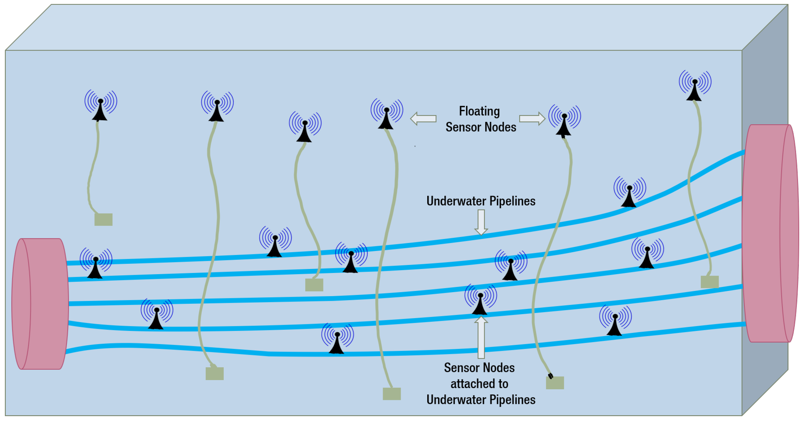
2.1.4. Underwater Pipeline Monitoring

Mohamed et al. propose a sensor network model for monitoring underwater pipelines which can be used for monitoring underwater marine cables, gas and oil pipelines [18]. Authors also compare different architectures for pipeline monitoring. This work also addresses the challenges like reliability, power consumption and also physical security of the network. Henry et al. propose a UWSN architecture for pipeline vandalization and oil spillage monitoring and detection [19]. This work also explored the viability, challenges and feature of these applications for implementing in Nigeria. The Security and deployment challenges of the wireless sensor nodes in the Niger-Delta oil and gas sector is addressed in [20].
Figure 1 presents a generalized underwater pipeline monitoring system with UWSN. Figure shows that, the static sensor nodes remain attached to the pipelines that are to be monitored. These sensor nodes collect the structural data of the pipelines and relay them to the dynamic floating nodes. Even though these floating nodes are allowed to move, they remain attached to the sea bed or floating buoy with strings to keep them in range. These floating nodes relay the data to the surface sink from where it reaches to the control center with RF communication.

2.1.5. Military Operations

Freitag et al. present an underwater wireless network for Mine Countermeasure (MCM) operation. It is one of the earliest efforts of MCM operation with Underwater Wireless Network. Authors use Autonomous Underwater Vehicle (AUV) with side scan sonar for mapping, identifying and classifying the target area [21]. Multiple number of AUVs can be used at the same time and they exchange information with themselves. Gateway buoys are located at the water surface and equipped with both acoustic modem and RF transceiver. These buoys allow the AUVs to be monitored from a distant operating station.

2.2. Background of UWSN

2.2.1. Underwater Acoustic Communication

Path loss designates the underwater acoustic communication. Mostly the transmitting distance and frequency of the transmitted signal define the path loss [22]. Absorption loss occurs when acoustic energy is transferred into thermal energy. This fact implies that the channel bandwidth has to be set on the basis of the desired transmitting distance. Absorption loss increases with the increase in the operating frequency and the interval between the receiver and the transmitter [22]. The power constraint automatically sets a limit on the availability of the bandwidth. Consequently, longer the communication link lesser the bandwidth, shorter the communication link more the bandwidth. Besides lower the bandwidth, lesser the data rate [23,24]. As for example, transmission over a distance of 30 km is feasible to perform by a single hop of 30 kHz bandwidth or the same transmission distance can be covered with much higher bandwidth of 300 kHz by 10 hops instead. So higher bandwidth (increased throughput) can be obtained by trading-off complicated relays in transmission. The shorter the bandwidth the longer the sensor transmission range. On the contrary, the transmission range decreases with the increases of the bandwidth. These variations in transmission ranges correspond to different bandwidths and operating frequency bands. The bandwidth of the underwater acoustic communication varies from less than 1 kHz to more than 100 kHz [2]. On the other hand, the operating frequencies for underwater acoustic channels usually vary from 10 Hz to 1 MHz [25]. Acoustic modems often use operating frequency bands centered at a unit of kHz which cover the distance on the order of kilometers (km) [26]. Besides, particular underwater applications need particular transmission range and bandwidth depending on the task it performs. The data rate of the acoustic communication varies from 31 kb/s to 125 kb/s depending on the channel encoding and the number of transmitters and receivers [27]. Table 1 presents the acoustic channels of UWSN in terms of operating frequency band, bandwidth, direct transmission range, and applications [2,25,26].
Opportunity for Free Space Optical (FSO) waves in the underwater environment is limited as the optical frequency band faces acute water absorption and heavy back scatter. Its attenuation is very high and it is almost 1000 times that of air even in the clearest water. Furthermore, the attenuation of the turbid water is one hundred times that of the densest fog [35]. So, in underwater environments, the main drawback of FSO is very limited transmitting distance due to high attenuation.
Acoustic communication can be considered as the most versatile underwater communication technique due to its low attenuation. Acoustic medium works out more perfectly with higher depth and steady temperature of the water. But in case of using acoustic waves in shallow water, temperature gradients and surface ambient noise can affect the performance adversely. Multi-path propagation due to reflection and refraction prospects might be another reason. Sound speed in water is 4 times than that of in air. But as the depth, temperature and Practical Salinity Unit (PSU) of water increase, the sound speed also increases [24]. Even though its speed in water is much slower than that of Electromagnetic (EM) waves. But it is the most reliable underwater communication medium which is feasible for practical deployment presently.

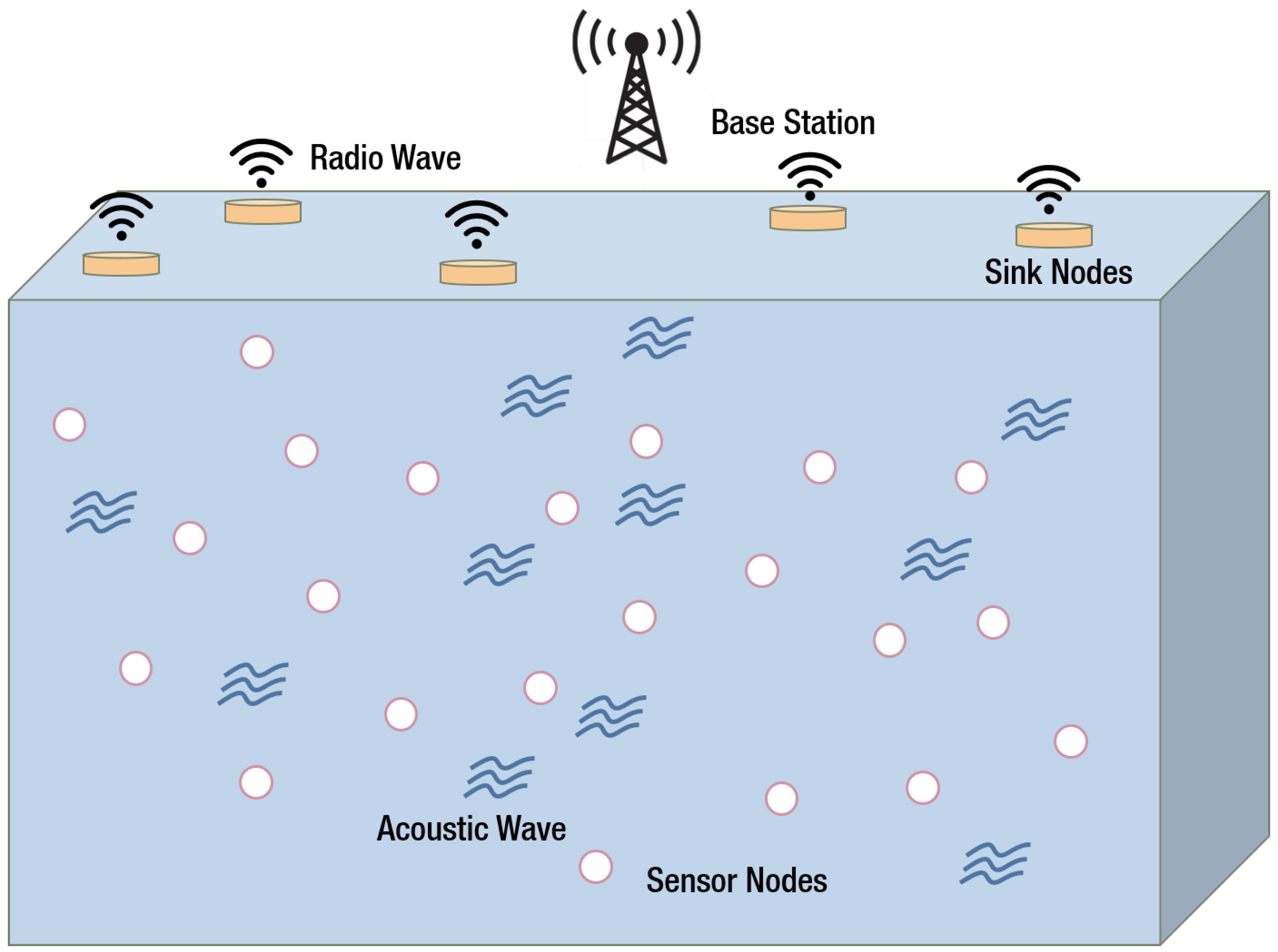
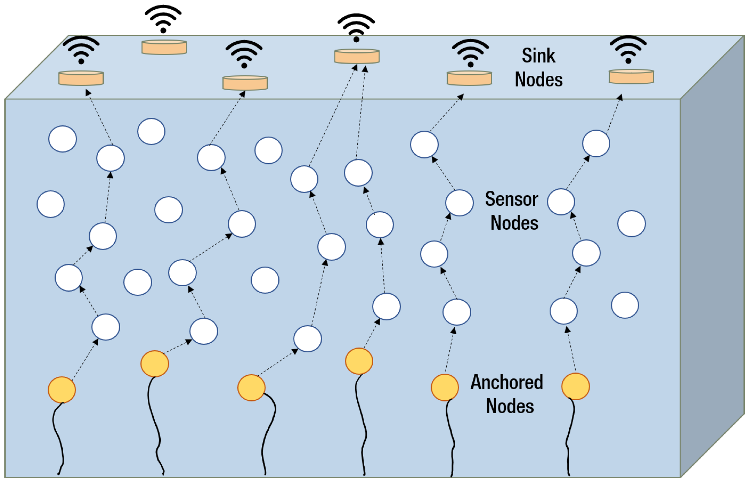
2.2.2. Deployment of Network Architecture

Underwater network is established to perform designated tasks. The network is formed by placing the multiple number of nodes at different depths of the sea volume to perform the task collaboratively. Every sensor node will transmit data by multi-hop or clustering technique to reach surface sink. In compared to terrestrial sensor network UWSN is more sensitive and complicated due to its three dimensional (3D) nature. Two communication architectures were proposed by Akyildiz et al. [2]: (i) Two dimensional (2D) network architecture, and (ii) Three dimensional (3D) network architecture.
When the network is 2D, sensors are remaining scattered only at the sea bed. These sensors can transmit data with each other. They can also communicate with the Underwater sinks (UW-sinks) via acoustic medium. UW-sinks send the extracted data from the sensors and send it to the sinks located at top of water surface. To perform this relaying, each UW-sink is provided with two acoustic transceivers- horizontal transceiver and vertical transceiver. Horizontal transceivers communicate with the deployed sensor nodes whereas vertical transceivers relay the data to the surface station. Vertical transceiver must be long ranged in case of deep ocean communication. These floating stations have the transceivers which can handle more than one links with the sinks at a time. These stations also have the facility to communicate with the onshore-sinks. Figure 2 shows a generalized two dimensional underwater network. Sensors are randomly spread in sea bed which collects the data and transfer it to the closest UW-sink. In 2D UWSN, the sensor nodes are deployed and placed only at the seabed. In this scenario, horizontal and vertical transceivers float at different depths of the sea to relay the data transmitted from the sensor nodes at the seabed to the UW-sinks. UW-sinks send the collected data to their respective horizontal transceiver. From horizontal transceiver data reaches to the surface sinks via long range vertical transceiver.
Whereas, unlike the deployment of sensor nodes in 2D UWSN, in the 3D UWSN, the sensor nodes are deployed and float at different depths of the sea level. The 3D UWSN is deployed to perceive the phenomena more precisely and thoroughly. The transmission of data in 3D USWN follows similar procedure with the help of different transceiver discussed in 2D UWSN.
But Akyildiz et al. proposed a slightly different idea in [36]. Authors suggested to tie each sensor-node to a surface buoy by a wire so that the depth of the sensor nodes can be changed by changing the wire length. By this, the sensor-nodes can be placed at different depth of the water levels with much ease. But these buoys can block the sea vehicles. Besides they are susceptible to weather tampering and pilfering.

2.2.3. Localization

Most of the applications of UWSN require time and location of the sensed data. So, localization is very important to perceive the network architecture and also to collect the data accurately [22]. Localization underwater is challenging because radio frequency is highly attenuated in underwater conditions, thus GPS technology is not feasible there. In most cases, the exact positioning of all the nodes is not necessary. Rather, the exact locations of a few nodes are enough and these are called the reference nodes. Such localization schemes are broadly of two types—(i) Range based scheme, and (ii) Range free scheme.
The range measurement is much more preferred when the acoustic channel is used instead of radio frequency or optical waves [37,38]. To locate a node in the network, a range based scheme utilizes distance, angular values, time stamps and difference of time for a packet received or sent. Whereas a range free scheme rather uses an anchor node as a reference for locating any node within the network [39]. Researchers like Luo et al., Ahmed and Salleh and Su et al. have surveyed these localization schemes elaborately in References [40,41,42] but only small-scale networks are compatible with these solutions. Erol et al. proposed the Dive and Rise (DNR) method for positioning [43]. It uses DNR beacons for localization of the sensor nodes. In this method, static anchor nodes are replaced by mobile DNR beacons. But the main downside of this method is that these DNR beacons are very costly and many of them are needed. Chen et al. reduced the expenses to a great extent by decreasing the requirements of DNR beacons [44]. They replace the DNR beacons with nodes of 4 separate kinds: (i) water floating-buoys, (ii) detachable transceivers, (iii) nodes that are attached to the bottom, and (iv) regular sensor-nodes.
It is presumed that the network is completely static and also the nodes of the network can measure the water levels. A pressure sensor always remains attached to this sensor nodes to perform this task.

2.2.4. Reliability

The main challenging factor for underwater networking system is relaying the collected data to the surface stations. Congestion control mechanisms of terrestrial networks show many difficulties in underwater wireless multi-hop networks [45]. TCP is the kind of mechanism that works based on an end-to-end connection technique. A TCP-handshake of the sending and receiving nodes is needed even before the transmission begins. In the case of UWSN, only a few bytes in each packet have to be transmitted. Transmitting this small data is a problem for TCP as it follows the 3 way handshake mechanism. In the case of acoustic communication, propagation takes longer than that of transmission which leads us to a bandwidth×delay product problem [24]. For reliability, TCP needs an end to end ACK and retransmission strategy but it will cause poor throughput along with a longer transmission time. It is considered in TCP that packet data losses are caused by congestion only. So, TCP only focuses on the decrease of the transmission rate but the error prone acoustic channel and the failures of the nodes can also be a reason for data packet losses in UWSN. So, to maintain throughput efficiency, the data transmission rate needs to not be decreased [24]. Other terrestrial protocols like User Datagram Protocol (UDP) usually do not maintain this flow control. Rather it just drops the packet without creating any scope for recovery or re-transmission which results in total loss of the data packet [45].
Data transmission in underwater communication is greatly affected by the following four challenging factors:
  • Noise of the Communication Medium,
  • Attenuation of the Channel,
  • Channel Bandwidth Limitation, and
  • Low Speed of the Acoustic Transmission.
The underwater noisy medium greatly degrades the transmission quality and there are four factors which cause this noise—1. movement of the Vehicles 2. waves 3. thermal variations and 4. other turbulence [46,47]. If ambient noise is designated by N in d B , then the power spectral density of the noise is as follows:
N = N v + N w + N tv + N tb ,
where,
N v = Power Spectral Densities of the Noises due to Movement of the Vehicles,
N w = Power Spectral Densities of the Noises due to Waves,
N tv = Power Spectral Densities of the Noises due to thermal variations,
N tb = Power Spectral Densities of the Noises due to turbulence.
And these parameters are modeled as follows [46]:
( 2 ) N v = 40 + 20 ( s 0.5 ) + 26 l o g ( f ) 60 l o g ( f + 0.03 ) . ( 3 ) N w = 50 + 7.5 s + 20 l o g ( f ) 40 l o g ( f + 0.4 ) . ( 4 ) N tv = 27 + l o g ( f ) . ( 5 ) N tb = 27 30 l o g ( f ) .
Here, f denotes the frequency in kHz and s denotes the speed of the wind where s [ 0 , 1 ] and it defines the extent of shipping noise. Noise of the ship movements ranges from 20-200 Hz whereas noise due to thermal variation affects the signals above 200 kHz.
Absorption loss and spreading loss cause attenuation in underwater communication. Attenuation also varies with the frequency of the signal and also the distance of the signal from the source [47]. So, the attenuation of the signal in the underwater medium is denoted by A ( d , f ) , where d is the distance of the signal from the source and f is the frequency of the signal. Equation (6) shows the expression for this attenuation where A c is the normalized constant, α is the absorption co-efficient and k is the spreading factor (in practice k = 1.5):
A ( d , f ) = A c d k α ( f ) d .
The delay efficiency of UWSN greatly depends on the speed of the acoustic waves. The speed of the acoustic waves in saline water can be expressed as [48]:
c = 1449 + 4.591 T 5.304 × 10 2 T 2 + 2.374 × 10 4 T 3 + 1.34 ( S 35 ) + 1.63 × 10 2 D + 1.675 × 10 7 D + 1.025 × 10 2 T ( S 35 ) 7.139 × 10 3 T D 3 .
Here,
c = Speed of the acoustic waves (m/s),
T = Temperature in °C and 0° < T ≤ 30°,
S = Salinity factor in Parts Per Thousand (PPT) and 30 ≤ S ≤ 40,
D = Depth of the sea in meters (m) and 0 ≤ D ≤ 8000.
Loss of the data increases with bigger data packets. On the contrary, the data overhead increases when the packet volume decreases. So, data volume affects the reliability directly. One thing worth mentioning is that, as the data volume gets larger, collision rates of the network also get higher. Therefore, larger data packets are preferable only when the link quality is good enough. However, it is already experimentally proven that data error rates also depend on the lengths of the packets [45]. Error control mechanism is a major issue in reliability. A successful transmission highly depends on the technique that are used for error control mechanism. Depending on the properties of the wireless channel, packet sizes are determined. For example, bad channel conditions require smaller packet size, error detection and re-transmission mechanism whereas larger packets are preferable for good channel condition. Moreover, channel access rates are affected by increase in packet sizes, thus the traffic on the channel is also affected which ultimately affects the data error rates. The underwater condition is very transient for wireless networking. So reliable and adaptive protocols are needed for successful transmission of the data packets which is also very challenging. Some networking protocols play a decent role in UWSN, which is analyzed in Section 3.

3. Routing Protocols for UWSN

Any routing protocol in UWSN depends on different metrics to route the sensed data from sensor node to the sink. The performance of the routing also varies depending on these metrics. For example, some routing protocols compare the RSSI values of the signals of its neighboring nodes and forward the data to the node that has better RSSI values. This type of routing protocol always maintains a good link quality while forwarding the data but it does not take energy balancing into consideration. Some other routing protocols may depend on depth information of the neighboring nodes while data forwarding. These protocols transfer the data to its neighboring node which has the lowest depth from the water surface. These type of routing protocols may have better energy efficiency and lower overheads as it always finds the shortest path to forward the data but their delivery ratio is usually poor as they always choose the distant nodes which may not always have good link quality.
As already mentioned, knowing the location information of the underwater sensor nodes is one of the challenging issues in terms of accuracy, energy and cost-efficiency. Some researchers have used the location information for defining their routing protocols whereas some other routing protocols do not need the location information of the sensor nodes to route the data from the source to the sink. Depending on whether the routing protocol needs the location information for routing or not, all the routing protocols can be divided broadly into two categories—1. Location-based scheme 2. Location free scheme [49,50].
It is also a fact that every routing protocol cannot address all the challenges and issues altogether. Rather, different routing protocols address different challenging issues and improve them. For example, some routing protocols perform energy balancing among all the nodes of the network which improves the network lifetime and does not create void holes in the network. Besides, some other routing protocols may emphasize the reliability and the data transmission of the network with highest priority ignoring the fact of energy balancing. So, all the routing protocols can also be categorized into a few types depending on which of the routing metrics they are emphasizing or featuring [46]. In this classification, one routing protocol can be listed in two or more categories if they feature more than one challenging issue but authors have classified the schemes mutually exclusively as the schemes surely prioritize one factor over another. Based on the features, all the considered protocols are divided into five types—protocols featuring node mobility, energy balancing, channel conditioning, energy efficiency and network void hole avoidance. Table 2 depicts the classification of the routing protocols based on both localization and the features they are offering. The listed protocols are described categorically with their working procedure, key features, improvements and shortcomings as follows.

3.1. Protocols Featuring Node Mobility

This category of routing protocols considers the dynamic nature of the sensor nodes and the movement thus consider the dynamic depth of the nodes while choosing the route from source to the sink. VBF, HH-VBF, DBR, CoDBR and VTPfall into this category. Even though DMBR falls in the category of energy efficiency and EEDBR falls in the category of energy balancing, they are discussed in this group along with DBR as they are the evolution of DBR. They give better performance in dense network in comparison to the sparse one. So, these routing protocols are deployed for the tasks like underwater pipeline monitoring, where the sensor density is high.

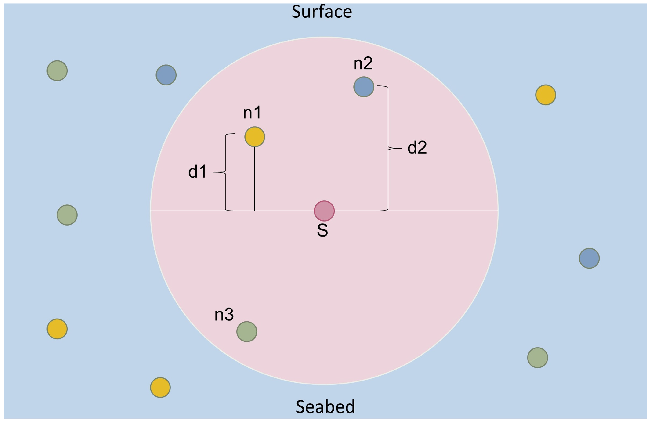
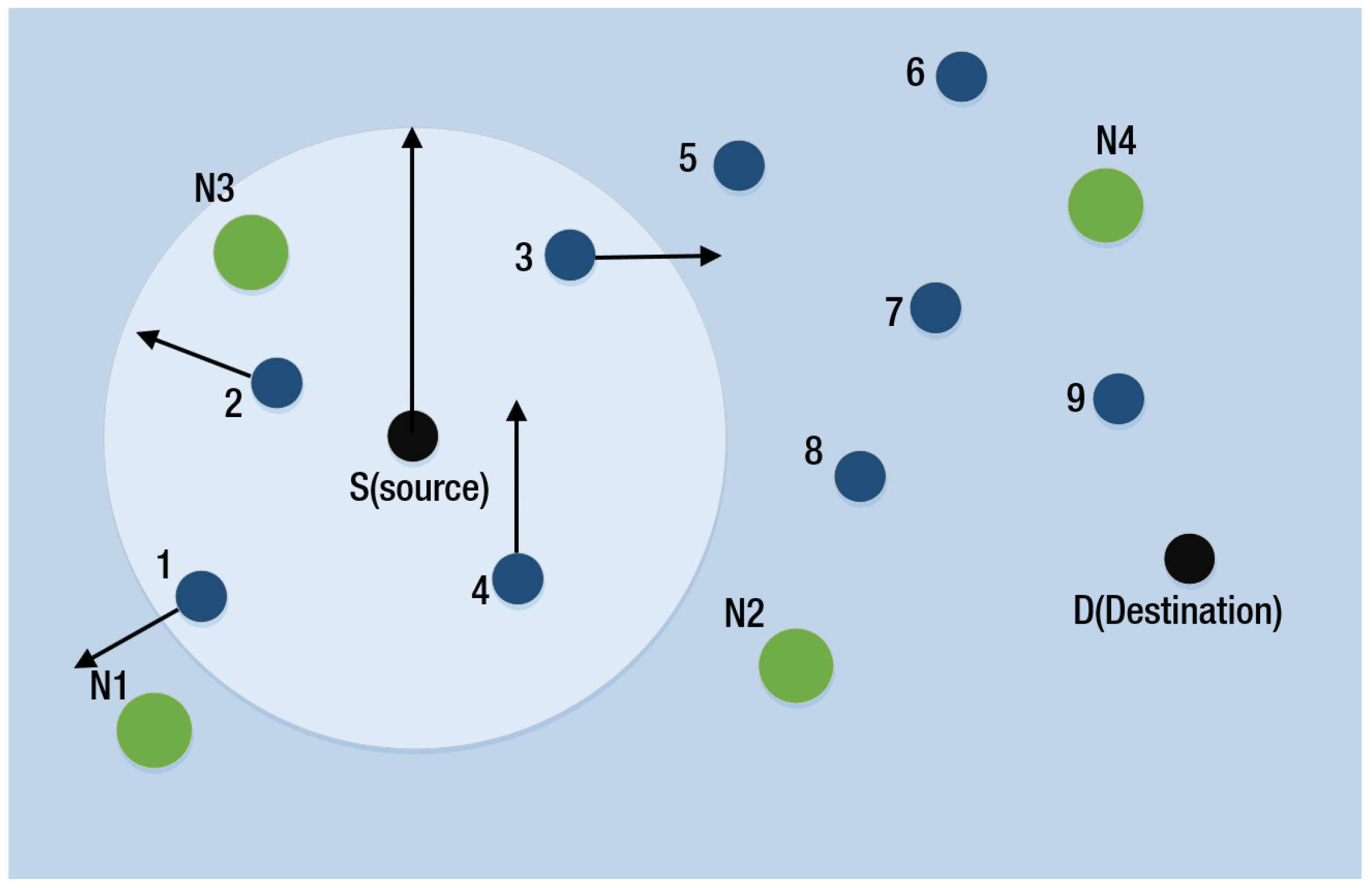
3.1.1. Vector Based Forwarding (VBF) and Hop-by-Hop VBF (HH-VBF)

UWSN is more challenging than the terrestrial network due to low bandwidth capacity, higher delay, 3-D nature, node mobility and transient nature of the medium. To cope with this issues xie et al. come up with a new protocol which is capable of making the routing sturdier, energy efficient, extensible [38]. This protocol is called Vector Based Forwarding (VBF). Here few nodes take part in the data transmission at a time where other nodes remain idle for that instant. So, state information is not needed here. This is a location based scheme. The location information of Sender, target and transmitting nodes are sent with each of the transmitting packet. Transmitting packet from source follows the ’routing pipe’ which is formed by all the forwarder nodes.
All the sensor nodes are well equipped for measuring the relative distance of the nodes. They also calculate the Angle of Arrival (AoA) of the receiving transmission. After receiving a signal, a node first calculates the AoA and the relative distance of the forwarder. The measurement of distance and AoA is done every time a sensor node receives the packet. Now, the forwarder node calculates its distance from routing vector. If distance is less than the presumed threshold value, only then forwarder node stores its calculated location to the data packet which is then forwarded for the next hop or else it just drops the data. If any node falls outside of the routing pipe, then those will not participate in the forwarding procedure.
In Figure 3, S1 is the source and surface sink is the target. The routing pipe is along the vector from S1 to the surface sink. W is the predefined threshold distance value. All the sensor nodes along this routing pipe act as forwarders during any data transmission but all other nodes sit idle for that instant which makes it an energy efficient one. As VBF does not require any state information, it is scalable to the network demand. It is energy efficient due to forwarding through the routing pipe only. Its data delivery rate does not depend on the stability on the neighborhood rather on the network density. In a dense network it gives a decent performance in delivery rate, average delay and energy consumption.
Even though VBF has some drawbacks. In VBF, routing path as well as the routing nodes are restricted by the virtual routing pipe. This pipe is extended up to the surface destination, originating from the source. In a sparse network, it may happen that no node lies within the predefined routing path, then it will not transmit the data to the sink even if it happens to have other paths outside of the routing pipe. It will decrease the packet delivery ratio drastically. As the node distribution is uneven in underwater environment, it is very troublesome finding the right radius threshold.
To overcome its short comings Nicolaou et al. proposed an improved protocol in which authors preferred per hop routing pipe for individual forwarder over the single pipe connecting sink and the source. It is called hop-by-hop VBF [51]. In this, every intermediate forwarder determines the pipe direction depending on its own position and the position of the neighboring nodes and the sink. So HH-VBF can always find a route in sparse region where there is a less number of neighboring nodes. Eventually HH-VBF gives better packet delivery ratio than VBF, especially in sparse regions. Yet, its routing pipe radius threshold can degrade its performance. Besides, it gives more signal overhead than VBF due its hop by hop forwarding.

3.1.2. Depth Based Routing (DBR), Depth Based Multi-Hop Routing (DMBR) and Energy-Efficient DBR (EEDBR)

Knowing the exact location of the sensor nodes is very difficult and also a critical factor of the underwater networking. Yan et al. presented a protocol where only the height of the sensors is necessary instead of the full-dimensional location information. This information can be achieved just by attaching a depth sensor with the nodes. These depth sensors are not that costly [52]. Several data sinks should be floating at the top of water body. This ultimately collects the data from the nodes deployed at different level of water.A node from the bottom of the water-body collects the data which act as the source. At first a node compares its height with the height of the prior sender from the bottom surface. Then it distributively takes a decision on packet forwarding. When the height of the node is higher than that of the sender, it considers itself to be qualified forwarder and will forward the data. Otherwise it just discards the packet because a node closer to the surface was its prior sender. This procedure continues until the packet reaches the surface. Reception of the packets by any of the surface sinks is considered a successful transmission. As the nodes closer to the surface is always chosen as a forwarding node, it consumes less energy and travels less distance. Figure 4 depicts the routing technique of DBR where S is the source. The range of the source S covers the neighboring nodes n1, n2 and n3. Here, a larger circle around source and forwarders depicts the transmission range of the source. Source broadcasts a data packet with its location information. Every node falling in the range of S receives the data to compare the depth of node S from the surface its own depth. Node n3 is discarded as its depth from the surface is higher than that of S. Here, both the nodes n1 and n2 are qualified forwarder and n2 is selected as the next sender as it is closer to the surface. Now, n1 just drops the packet and n2 broadcast the data in the previous way to find the next sender. This is done recursively until the packet finds any of the surface sinks.
The authors introduced a global parameter called depth threshold to control the number of nodes needed to send the data packet. A node forwards data only when it finds that difference of its own depth and earlier hop’s depth are greater than that of threshold value. If the threshold value is high, energy consumption will be less as the nodes involving in data packet delivery will be less but it will cause low packet delivery ratio. On the other hand, setting a higher threshold value will involve a larger number of nodes delivering the same packet data and eventually increase the energy consumption. This will result in a high packet delivery ratio. So, depth threshold value is the key to the trade off between the energy consumption and delivery ratio. Though it gives very good performances in dense network, in sparse areas packet delivery ratio degrades as it works only in greedy mode. Simulations show that, it can perform up to 95% of packet delivery ratio in dense network with reasonable amount of energy consumption [52]. Furthermore, DBR is improved in Depth Based Multi Hop Routing (DMBR) which includes multiple sink network structure [62]. DMBR divides the whole process into two steps—route discovery and send packets, which makes the routing scheme more energy-efficient and also reduce the channel conflicts, thus improving DBR. It was improved further in Energy Efficient Depth Based Routing (EEDBR) [55]. Wahid et al. suggested to improve the life time of the network by utilizing the sensor residual energy. In DBR, a node having smaller depth than neighboring nodes will always forward the data in each and every transmission whereas nodes having slightly larger depth may sit idle. As a result, same nodes will be used repeatedly and eventually die out earlier than the other nodes. This creates routing holes all over the network which partitioned the network into parts. As a result, sensors can not communicate which results in shorten the network life time. This was improved in EEDBR. In EEDBR every sensor node shares its residual energy and depth with its neighboring nodes. Besides, each sender also broadcasts the depth of its neighboring nodes during transmission. When forwarding nodes receive the data packets, depending on the residual energy it stores the data for a specific period and to maintain the required delivery ratio, nodes take decision whether to transmit or suppress the packet transmission. DBR reduces the delay and improves the network lifetime. Moreover, it gives a satisfactory delivery ratio of the data packets along with good power-efficiency.

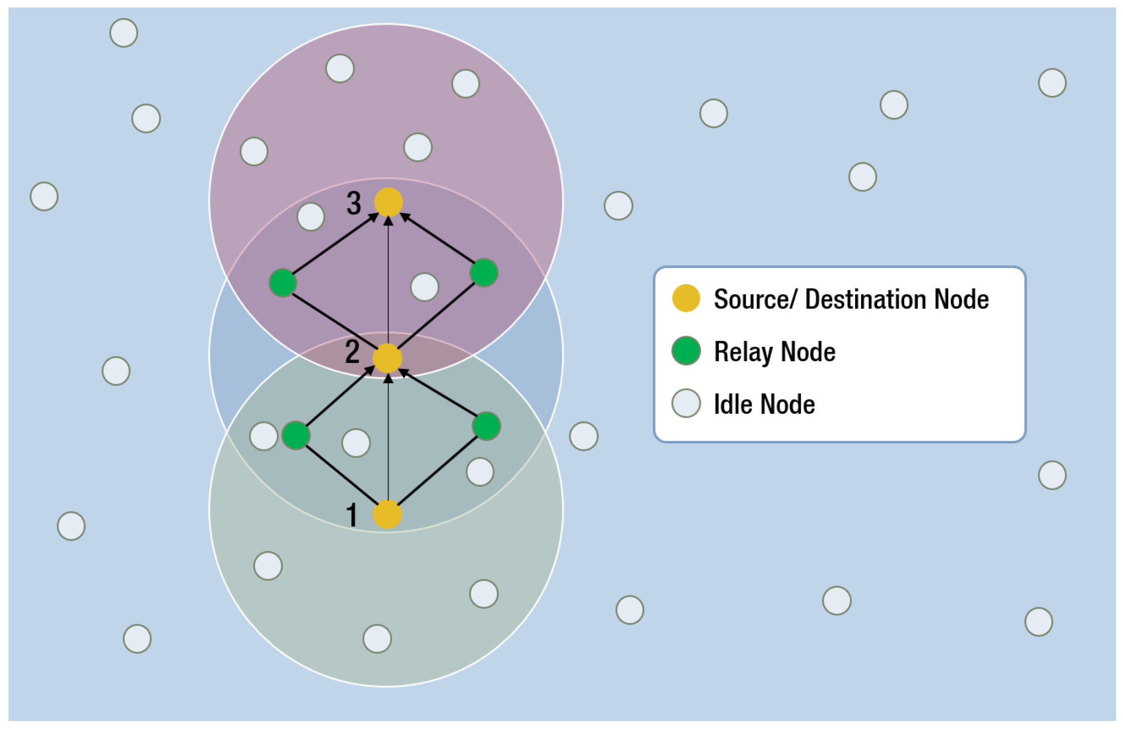
3.1.3. Cooperative Depth Based Routing (CoDBR)

Incorporating co-operation with an existing routing protocol called DBR, a unique scheme called cooperative DBR (CoDBR) has been proposed by Nasir et al. The main aim of this protocol is to improve reliability and throughput [54]. In DBR, a source node broadcasts the data to its neighboring node. These neighboring nodes compare their depth with their respective previous hop distance and a forwarder is selected on the basis of minimum depth. By recursion of this depth based single link procedure, eventually data from source reaches to the surface sinks by multi-hop. But this technique is prone to high bit error rate and low reliability due to multi-path fading, noisy underwater environment and hindrance posed by marine life. So, authors suggested Cooperative Path diversity via multiple paths to subdue this problem in CoDBR.
CoDBR is also a localization free protocol like DBR which only needs to know the depth of the sensor nodes. Every node has the depth information of their neighboring nodes. A source node compares the depth of its neighboring nodes and the node with the minimum depth is selected as the destination for the next hop. The nodes with the second and third lowest depth are selected as relay node. CoDBR has two phases—(1) path setup (2) data transmission. A cooperative multi hop path is established from source to the sink in the first phase. Data transmission in Co-DBR is explained by Figure 5.
All the black and blue nodes of the figure take part in the data transmission whereas the gray nodes remain idle. Node 1 is the source and it sends the data to the node 2 as next hop. The blue nodes relay the same data from node to the node 2. This improves the reliability and reduces the bit error rate of the transmission. If the sink is within the range of the source node, then the sink becomes the next hop destination. If the sink is not within the range of the source then, source node selects next hop destination from its neighbor on the basis of the lowest depth recursively until the source node finds the sink as its next hop destination. Moreover, in both the cases two relay nodes are selected for simultaneous transmission of the same data to the destination. In data transmission phase, data is transmitted to the sink through multi hop paths which was established in path setup phase. Source node broadcasts its data to the next hop destination node and relay nodes. Relay nodes employ Amplify and Forward (AF) technique to deliver the received data to next immediate destination. Relay nodes do not forward their own sensed data rather they only amplify the data received from the source and send it to the next destination. Upon receiving these three independently faded copies of data at the next hop destination node are merged together by maximal ratio combining technique. If the Bit Error Rate (BER) of the received data crosses the threshold value T, the data packet is simply dropped. T is the maximum allowable Bit Error rate. This is done recursively until the data from the source reaches the sink. As a two relay node also transmits along with the source node, CoDBR has the higher reliability than DBR but the energy consumption of CoDBR is higher than that of DBR. It leads to shorten the network life of CoDBR significantly. In comparison with DBR, it offers 83% more throughput and 90% less packet drop. But due to relay nodes it incurs higher power consumption and higher delays. This trade off must be considered to get higher reliability. Its data delivery ratio can be improved further, if the destination node asks for re-transmission, in case the BER of the received data crosses the threshold value instead of just dropping the data. This will improve packet delivery ratio and throughput as well. It is also noticeable that relay nodes do not send their own data to the destination at a time in one round. Throughput can be increased further if they can send their own data and the relaying data together to the destination node in a single round.

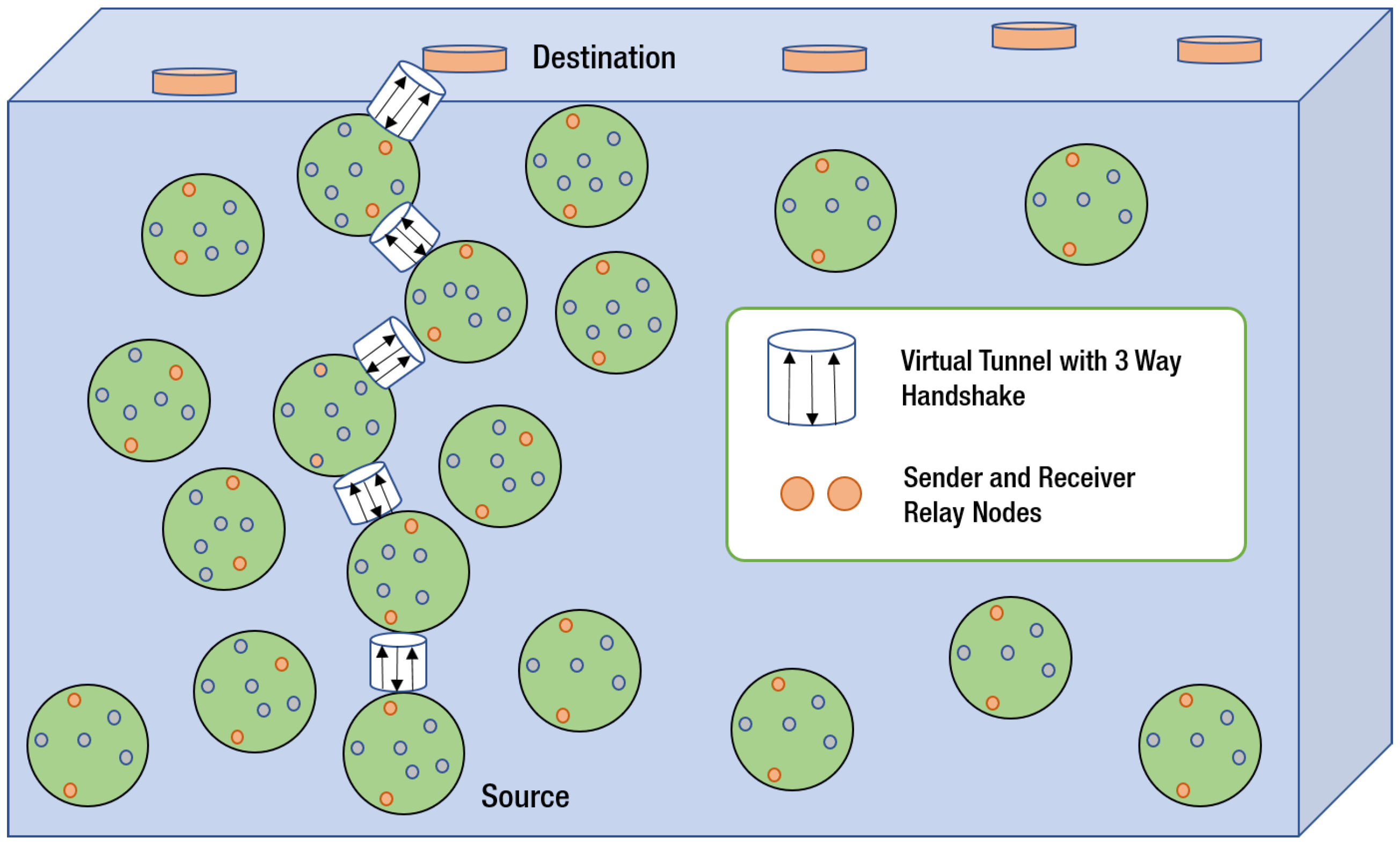
3.1.4. Virtual Tunneling Protocol (VTP)

With an aspect of improving the energy consumption, Packet Delivery Rate (PDR), transmitting path and latency, Bharathy and Chandrasekar proposed Virtual Tunneling Protocol (VTP) for UWSN [53]. There are three main steps in VTP: (i) choice of nodes for relay, (ii) tunneling to the destination from source, and (iii) packet transmission through tunnel.
It is a cluster based protocol where all the nodes arrange themselves in several groups. Sinks are floated on the surface of the water which acts as the destination. All the clusters in the way of source to the destination is taken into consideration. Each cluster sends data from one to another towards the destination until the packet reaches any of the sinks. Two border nodes from each cluster are selected as relay nodes- one for receiving the data and one for sending it. Border nodes and the nodes which have transmitted the latest data packet are given the highest priority for being the relay nodes. In this way, the selected groups with their relay nodes form a virtual tunnel from source to the destination with good link quality. The collected data from the source is sent continuously to the destination through this tunnel. The transmission follows three-way handshake like TCP. Figure 6 explains the data transmission process of VTP in details.
The figure shows that a virtual tunnel is formed from source to the destination. This tunnel transfer the data from one cluster to another depending on its distance to the sink. This follows three-way handshake between the relay nodes. Due to the thee-way handshake and tunnel formation, a strong link is formed from the source to the sink (destination). Authors showed that, VTP gives better result in Packet Delivery Rate, latency and number of hops in compared to the Channel Aware Routing Protocol (CARP) and multi-level Q-learning based routing protocol- MURAO [66,67]. But this protocol do not show any results on energy-efficiency, reliability and overall performance. Moreover, VTP might not be energy conservative as it performs three-way handshake for single packet transmission.

3.2. Protocols Featuring Energy Balancing

All the sensor nodes in UWSN are battery powered. So, energy balancing is one of the important factors while determining the route to the sink. Otherwise, it is most likely for some nodes to be overburdened in comparison to others thus discharge faster than other. This create holes in the network creating serious disruption in the network. RE-PBR and EEDBR does the energy balancing which ultimately improve the reliability and network lifetime. These routing schemes can be utilized in applications like natural hazard detection, where the reliability and network life-time is the most critical issue.

Reliable Energy Efficient Pressure Based Routing (RE-PBR)

Khasawneh et al. propose Reliable Energy Efficient Pressure Based Routing (RE-PBR) to improve energy efficiency of the routing. Moreover, it does not need location information of the nodes for routing. It takes the link quality and depth into account along with the residual energy for reliable transmission [56]. The scheme architecture is depicted in Figure 7. The network comprised of base station, sinks and underwater wireless sensors. Underwater sensor-nodes are provided with acoustic modem and pressure sensors which are placed in different depths of sea. The vertical movement of these nodes are negligible whereas the parallel motions are considered upto 0–3 m/s [52,68]. Sinks are placed at the top of the water. All the nodes aggregate the data and deliver it to the sinks. As the nodes are placed at different depths of the sea, they employ multi-hop technique to deliver the data to the sink. The main feature of RE-PBR protocol is that, it measures link quality precisely with triangle metric in its forwarding process. No other depth based routing protocols have used triangle metric to find the link quality during data forwarding.
Every node aggregates information like ID, remaining power and depth in a data packet. This data packet is sent to each of its one hop neighbor. So, each node can compare its own distance from the surface with that of sender. If the depth of the sender is more than its own depth, the node saves the data of the hello packet. Else, the data packet is discarded by the node. In this way, each node collects the data of one hop neighbor and stores them to select the best forwarding node. Then by computing the distance, the link quality based triangle metric is estimated for each stored data. Two things are considered while selecting the next forwarding node—route cost basing on the residual energy and the distance which depends on the triangle metric. Nodes eventually repeat this process till the data finds any sink for transmission.
The network lifetime of RE-PBR is longer when compared with DBR and EEDBR. This is because in RE-PBR the forwarding node is chosen depending on their higher residual power and better link quality. The packet delivery ratio of RE-PBR is also better than that of DBR and EEDBR. Moreover the energy efficiency of this scheme is better than that of DBR and EEDBR. As there is no provision for holding or storing the data, the delay is also minimal in this routing protocol.

3.3. Protocols Featuring Channel Properties

These routing protocols are designed to achieve better channel properties like better link quality, better Signal to Noise Ratio (SNR), less noise or less attenuation. These will greatly improve the reliability and delivery ratio of the network. This category includes DFR and LARP. As they maintain the desired link quality all the time, their preferred application is distant controlling of AUVs as like [21].

3.3.1. Directional Flooding-Based Routing (DFR)

For improving the reliability, Shin et al. proposed Directional Flooding Based Routing (DFR) [57]. Authors suggested to consider larger number of nodes to achieve better reliability. These few more forwarding nodes make the data packets reach to the sink reliably. The forwarding activity is performed per hop. Few researchers have already worked on flooding based routing but Shin et al. have the most prominent research work on DFR [57,69]. The authors suggested broadcasting a data packet by way of a source node that has its own location information and one other parameter. This parameter contains an angle known as a base_angle which is set to its predefined minimum value according to network density. Upon receiving a packet, the node measures an angle between two vectors-from source node to itself and from itself to sink and this angle is called current_angle. When node receives a packet it compares base_angle with current_angle and decide whether to forward a packet. If the node’s base_angle is bigger than that of current_angle, it is considered as out of flooding scope and it is discarded. In reverse case, base_angle is adjusted so that it can maintain link quality with the nearby nodes. Two conditions must be satisfied by all the nodes to maintain the link quality, that is, (i) the current_angle of the neighbors must be larger than that of current_angle of the forwarder, and (ii) the distance of the neighboring nodes to a sink must be less than that of the distance of the forwarder to the sink.
Nodes will not transmit packet until the above conditions are fulfilled. The forwarder node then broadcasts the packet with a source location and a new base angle. Packet transmission in DFR is shown in Figure 8.
The source S broadcasts a packet with its location and base_angle whose value is set to A_min. When F receives the packet, it compares its current_angle (angle between F S and F A ) with the base_angle. F adjusts its base_angle with B and C according to the average link quality in case the current_angle is larger than base_angle. It then floods the packet with the adjusted base_angle and its location in it, otherwise it just drops the packet. Simulations have shown that DFR gives a better delivery ratio compared to VBF. Moreover, it offers 73% shorter end-to-end delay and 43% less communication overhead than VBF, even though it has some drawbacks. When the sink finds no node in its range, then a hole is created in the network which may disrupt the network.

3.3.2. Location-Aware Routing Protocol (LARP)

Even though existing routing protocols have improved UWSN drastically, they still pose many problems. Shen et al. proposed a novel routing protocol which gives a better performance in delivery ratio and reduce overhead in compare to all other existing routing protocols. This is called Location-Aware Routing Protocol (LARP) [58]. It adopts a Received Signal Strength Indicator (RSSI) method to know the location of the nodes [70] and it utilizes this location information of the nodes for the packet data transmission. It is considered that there are two kinds of nodes in the network-(1) anchor nodes (2) general nodes. Anchor nodes are the reference nodes and are used to determine the location of the other nodes. Anchor nodes are equipped with GPS module which broadcast the location information to the beacon. It is considered that anchored nodes have- (i) the property to know the precise location of the anchor nodes by GPS technology or other methods [71], (ii) enough energy and storage capability, (iii) enough RF transmission range to cover the whole network scale, (iv) the property of random mobility.
With the help from 3 or more anchor nodes, a general node usually finds its own positioning and they save their positioning information. If these general nodes come near to any anchor node, they transmit their location information to the anchor node to store. Figure 9 depicts data transmission of LARP where N1, N2 and N3 are anchor nodes. S is designated as source and D is designated as destination for the transmission. At first, the source node looks for an anchor node within its range or waits for any anchor node to come within its range. Source node requests for the destination node location to the anchor node. When anchor node broadcast the destination ID, all other anchor nodes will check that if there is destination node D within their range. If any of the anchor nodes find the destination node, the source node will get the information about the destination node.
Now the node S will broadcast the ’destination location’ request within its range. If the destination node D is within the range and receives the destination location request, it will reply to the node S. After that, node S will directly transmit to node D. Note here that, no other node will reply to the request upon receiving. When the source node gets no reply, the source node broadcasts ’moving direction’ requests. Moreover, Source node S collects all the information of the nodes within its range. Now the node which is moving in the direction of D, reply to node S. In the next step, the data packet is delivered to that particular node. Thus, the next best hop is selected. If it happens that, there are more than one node which is directed towards the destination D, then their speed is taken into consideration. The node with the greater speed is chosen as the best hop.
If it happens that there is no node directed towards the destination node then no node replies back to the node S and it waits until it gets any suitable node to make it the next best hop. In Figure 7, node 3 is selected as the next hop. In this way best hop is selected recursively until the data packet is delivered to the destination node. Simulations show that LARP gives a decent packet delivery ratio, lower normalized overhead. Moreover, it gives more reliable transmission than the other routing protocols even though it possesses some drawbacks. It needs a very dense network to work perfectly, besides a source node had to wait for an indefinite time if it does not get any anchor node within the range. It may also happen that the source node may have to wait for a long period of time to get a node which is directed towards the destination node to select it as the next best hop.

3.4. Protocols Featuring Energy Efficiency

One of the challenging issues of the UWSN is the limited energy source. So, these routing protocols work on achieving better efficiency in energy thus improving the lifetime of the network. This group includes FBR, DUCS and SEEC. These routing protocols emphasize the energy consumption of the nodes which eventually increases the network life-time. So, these are most suitable for environmental monitoring which needs deployment for longer periods.

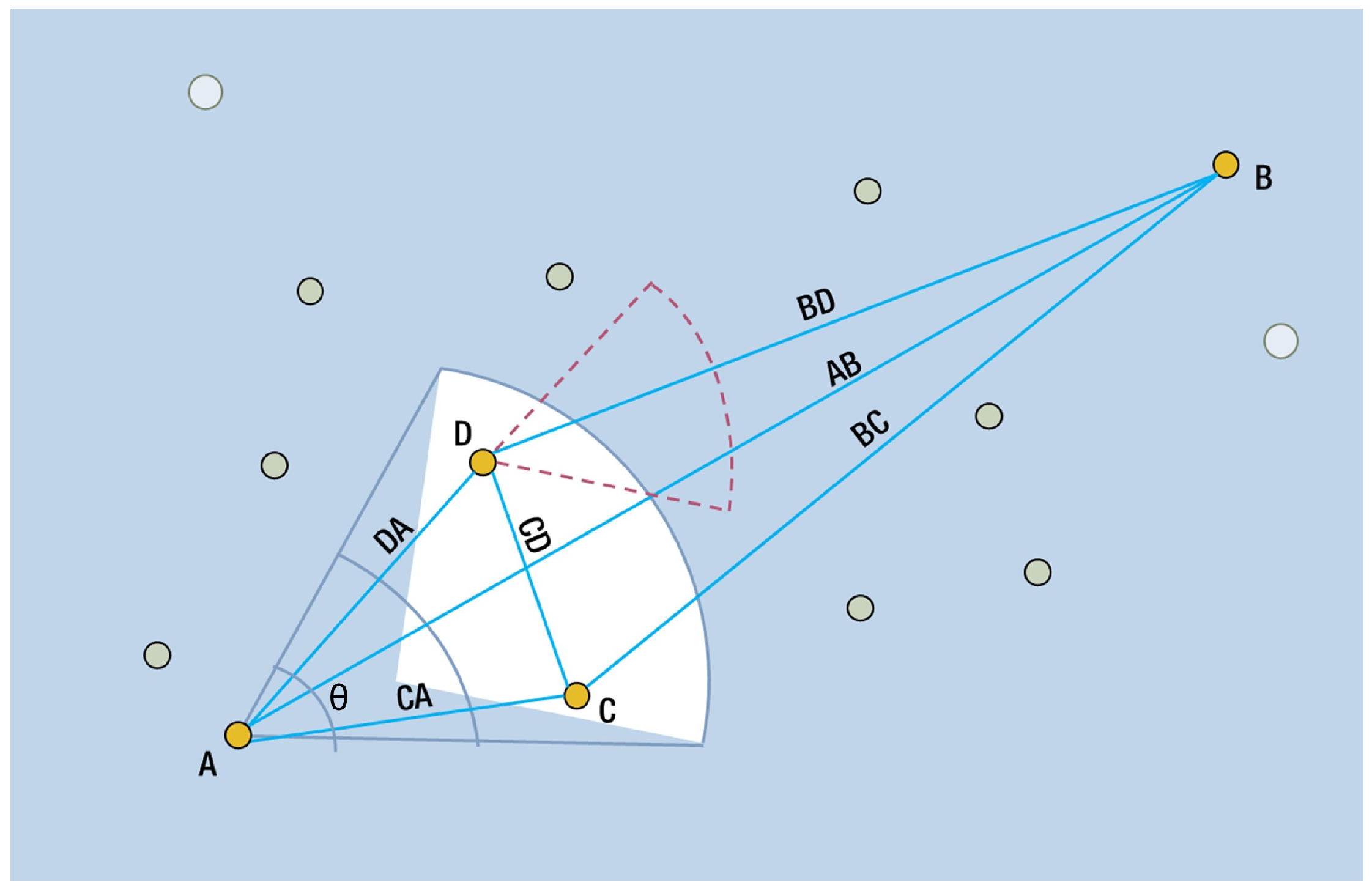
3.4.1. Focused Beam Routing (FBR)

To avoid unnecessary flooding of the data, Jornet et al. proposed a noble routing scheme called FBR [59]. FBR is suitable with both the static nodes and the moving nodes of the network. Moreover, the network with FBR needs not to be synchronized with global clock. Just by knowing the location of the source and destination a successful transmission is possible irrespective of the location information of the other nodes. FBR performs flooding for routing data packets and this flooding is restricted by the transmission power. To minimize the energy consumption of the network, this protocol engages different power levels for transmission. Figure 10 explains how a data packet is being forwarded in FBR. Node A is the source and node B is the destination where node A sends a multi-cast request to its neighboring nodes. This is called an RTS packet which holds the positioning data of node A and B. The lowest power level has the minimum range and range area increases when we switch it to a higher power level. But switching of the power level only occurs when it can not find any node within the designated rage for the next hop. But receiving nodes do not decide which power level to be used instead open loop power control and power level is decided by the transmitting node. It is also considered that there are definite power levels ranging from P1 to PN which can be increased from one level to the upper level when needed [72]. The nodes have to be within the perimeter of the defined power level to receive any detectable signal. Now the locations of the nodes which receive the multi-cast RTS earlier from node A is determined.
This location is relative to the line AB. The nodes that lie within the angle ± θ /2 at the source node A are selected as the eligible nodes for forwarding. If a node is eligible, this will respond to the received RTS. But in real life FBR may face some difficulties. First, due to transient state of the underwater condition and due to heavy current it may happen that, no node is within the cone of ± θ /2. Sometimes it may happen that some of the eligible nodes remain outside of the forwarding cone angle. In this case it can not find the eligible node for the next hope within the forwarding zone, source node needs to rebroadcast the RTS. Thus the overhead will increase which eventually disturbs the transmission. The sink is considered to be fixed here which makes the network more restricted.

3.4.2. Distributed Underwater Clustering Scheme (DUCS)

Batteries are the power source for the sensor-nodes which are difficult to recharge or replace. So limited energy is a major constrain for UWSN. Domingo and prior presented DUCS which is—(1) energy-aware (2) non-time-critical (3) self-organized and (4) provides random node-mobility [60]. A distributed algorithm is used to form the clusters. It is assumed that sensor-nodes constantly generate data which needs to be transmitted. Moreover, these nodes have the capability to change the transmission power level whenever necessary. It uses a self-organizing technique to form local clusters each having one cluster head. All the cluster members transmit their data to their respective heads by single hop transmission. After accumulation of all the data, cluster heads sent them to the sink. But this transmission from cluster-head to the sink is completed by multi-hop communication. Cluster heads control the communication within its own cluster and also the inter-cluster communication. These cluster-heads are chosen randomly from the cluster members on the basis of regular rotation. So, it makes this protocol an energy efficient one. Besides, to avoid fast battery-drainage of the cluster-heads, DUCS allows randomize change of the cluster heads withing the cluster members. The function of operation is divided into two rounds. First is called setup in which clusters are formed and the second round called network operation which completes the data transmission. A series of data are sent from the member-nodes to the heads which maintain a particular routine. This series of data are called frames. Member-nodes sent several such frames to their own heads of the clusters during second round. Simulation of DUCS has shown that—(1) its packet delivery ratio is high (2) network overhead is reduced (3) its throughput increases consequently. Though it has some performance issues, DUCS is energy efficient. The cluster structure can be affected by the movement of the nodes due to water current which may lead to decrease cluster life. It is worth mentioning that, only a cluster head can communicate with another head and this is possible only in the second round. So if by any means these heads are distant-apart such far that they can not communicate directly, even then they can not communicate through the non cluster heads present in between. This can interrupt the network drastically and hamper the life-time as well as performances.

3.4.3. Sparsity-Aware Energy efficient clustering (SEEC)

In schemes like DBR and EDBR, two things are considered while choosing the next forwarding node during routing. These include how close the nodes are to the surface and their remaining power. This creates several coverage gaps which affects the life span of the network badly. Thus, for improving network lifetime along with stability and energy efficiency Azam et. al propose a unique scheme called SEEC [61].
Here, depth finding modules are attached to every randomly scattered sensor node of the network. The whole network region is divided into a few sub regions of equal areas. The denser regions of the network are sorted out on the basis of a novel algorithm for finding the denser regions. Similarly, with another dedicated algorithm the sparse areas are also found out. Sinks are used to collect the data from the sparse areas. On the other hand, a clustering scheme is employed to extract the data from the denser areas. On the basis of lower depth and high residual energy, one of the nodes from each cluster is selected as the cluster head. This head has to be the closest node to the water surface in compared to the cluster members. Moreover, its residual power has to be more than the average residual power of the clustering nodes. Data transmission in dense region is completed in three layers. At first the data is collected and aggregated from the member nodes. After that, it is sent to their respective heads. At last, all the heads of the clusters send this data to the nearby static or mobile sink. In the case of the sparse region, two moving sinks are used to extract the data from the nodes. For better understanding, these two sinks are supposedly being designated as MS1 and MS2. One of these two sinks (MS2) remains fixed at the most sparse areas. Other sink-MS1 travels from the topmost sparse areas to the least sparse areas in every round. It is mentionable that region of MS2 is not under the consideration of MS1 mobility and MS2 remain fixed in its position until the death of each node of the region. After that MS2 moves to the topmost sparse region for the rest of the sparse nodes. These sinks always choose the center position of the whole region to travel. By this they can cover the maximum number of nodes within their transmission range. Mobile sinks move from one sparse region to another sparse region periodically and eventually collect the data from all the sparse regions. SEECemploys the moving sinks for the sparse areas where it uses clustering schemes for the dense network. This makes this scheme to be more energy efficient than other two schemes like DBR and EEDBR. Moreover, SEEC also shows a longer life-span and give a better packet delivery ratio than these two mentioned schemes. More over, clustering technique gives SEEC a better stability period but it has lower throughput than DBR and EEDBR.

3.5. Protocols Featuring Network Void Hole Avoidance

Most often UWSN has to cover some vast area and it might happen that, sender node can not find any neighboring node in its range to forward the data. This network void hole is created due to the random placement of the sensor node, dead neighboring node or water movement may take all the neighboring node out of the range of the sender. Performance of the whole network is greatly hampered due to these void holes. These routing protocols address this challenging issue to avoid network void holes. EBER2, WDFAD-DBR, VSM and RSM fall into this category of the UWSN routing protocols. These schemes are suitable for a sparsely populated network where the deployment covers a vast area.

3.6. An Energy Balanced Efficient and Reliable Routing Protocol (EBER2) and Weighting Depth and Forwarding Area Division DBR (WDFAD-DBR)

An Energy Balanced Efficient and Reliable Routing Protocol (EBER2) has been proposed by Wadud et al. to achieve improved energy balancing, reliability, energy efficiency, network latency and packet delivery ratio [63]. Unlike DBR, Weighting Depth and Forwarding Area Division DBR (WDFAD-DBR) considers depth of the both current hop and expected forwarding hop thus avoid the void holes [65]. But WDFAD-DBR still faces void hole issues as it does not consider Potential Forwarding Nodes (PFNs) for the second hop. WDFAD-DBR also increases duplicate packets and packet collisions which affects the energy efficiency and lifetime of the network [63]. Wadud et al. in EBER2 solved the problems posed by WDFAD-DBR. EBER2 is formed of three types of nodes, that is, (i) sink nodes, (ii) anchored nodes, and (iii) relay nodes.
Figure 11 shows the network architecture of EBER2. Anchored nodes remain attached at the bottom of the water level and remain fixed in their positions. The sensor nodes or the relay nodes are deployed at a different layer of water levels which are movable. The relay nodes sense the surrounding data and also act as a forwarder node to transfer the data. The sinks remain floated at the water surface and are considered as the destination.
The depths of the first two hops are considered for selecting the forwarder node which decreases the chance of the void hole issue in the network. The residual energy of the nodes is also considered. It is used to avoid duplicate packets by taking higher values of the holding time of the forwarding nodes. This allows energy optimization by avoiding duplicate packets thus increasing the packet delivery ratio. Moreover, the use of residual energy as a metric for selecting the forwarder node enables energy distribution in the network. This eventually prolongs the network lifetime. To address the issue of reliability, PFNs of the next forwarder are also taken into account which also decreases the probability void holes in the network.
The energy consumption of the nodes nearer to the sink is always higher due to higher network traffic. If these nodes die earlier it would cause the network to be separated from the sinks. To address this problem, these nodes tune their transmission power level according to the distance to reach the nearest sink. Simulations show that, the EBER2 performs better in energy efficiency, PDR, and packet loss when compared to WDFAD-DBR. But this protocol increases the end to end delay between the nodes by considering the residual energy.

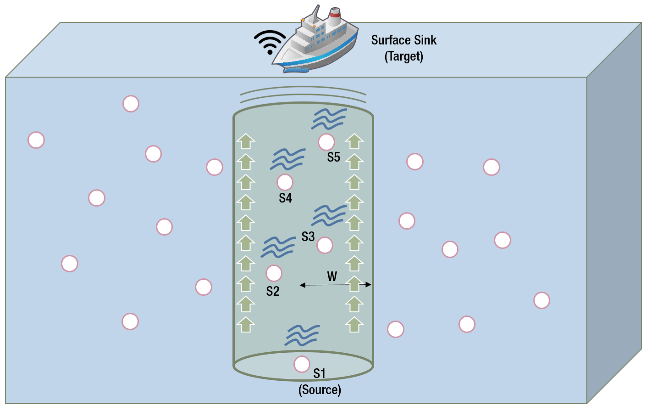
3.7. Regional Sink Mobility (RSM) and Vertical sink Mobility (VSM)

In SEEC, the throughput was low due to multi-hopping of the clustering head in the dense region. To increase the throughput Ali et al. proposed two routing protocols. One is called the Regional Sink Mobility (RSM) where the sinks move regionally to extract the data. Another scheme is called Vertical Sink Mobility (VSM) in which the sink travels vertically to collect data from the nodes [64]. In both the schemes, it is not needed to know the information of each and every node rather one node needs to know the information of its neighboring nodes.

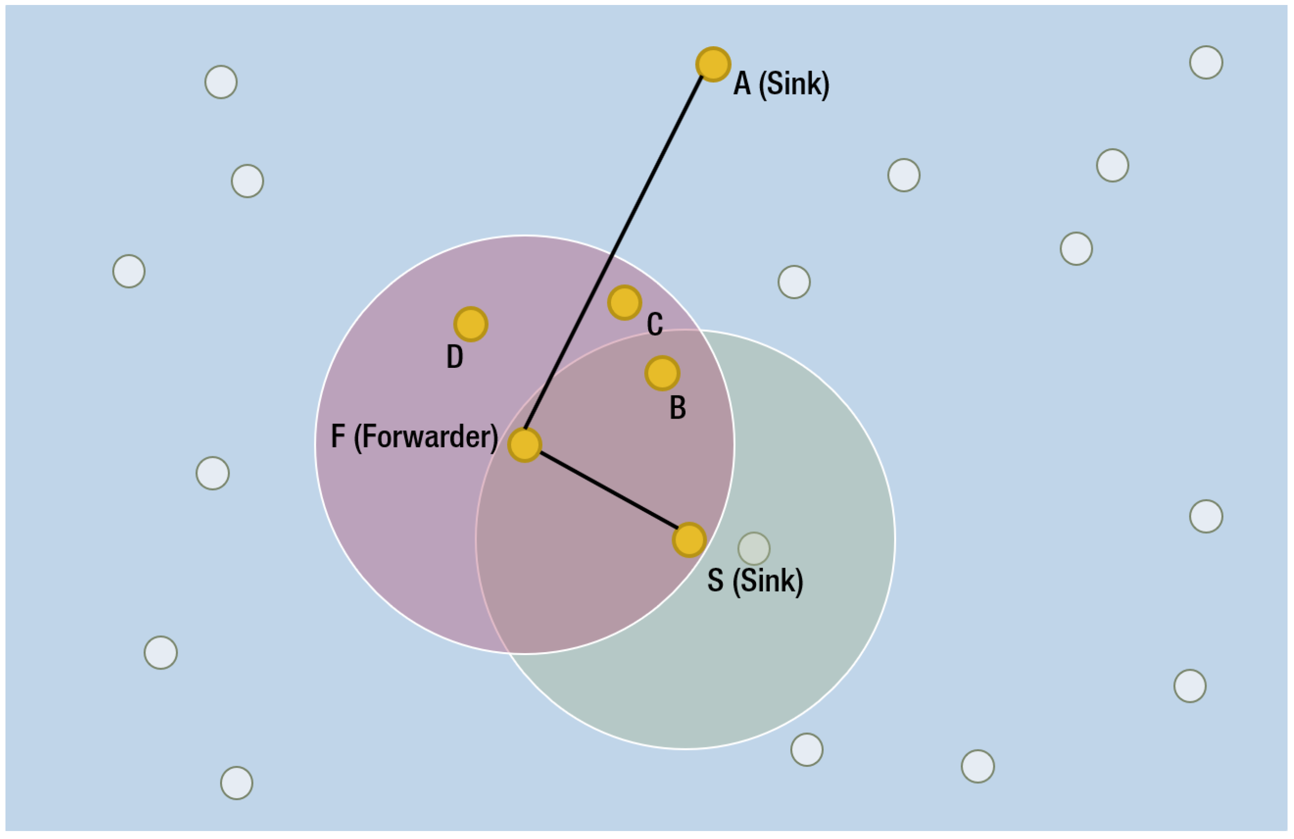
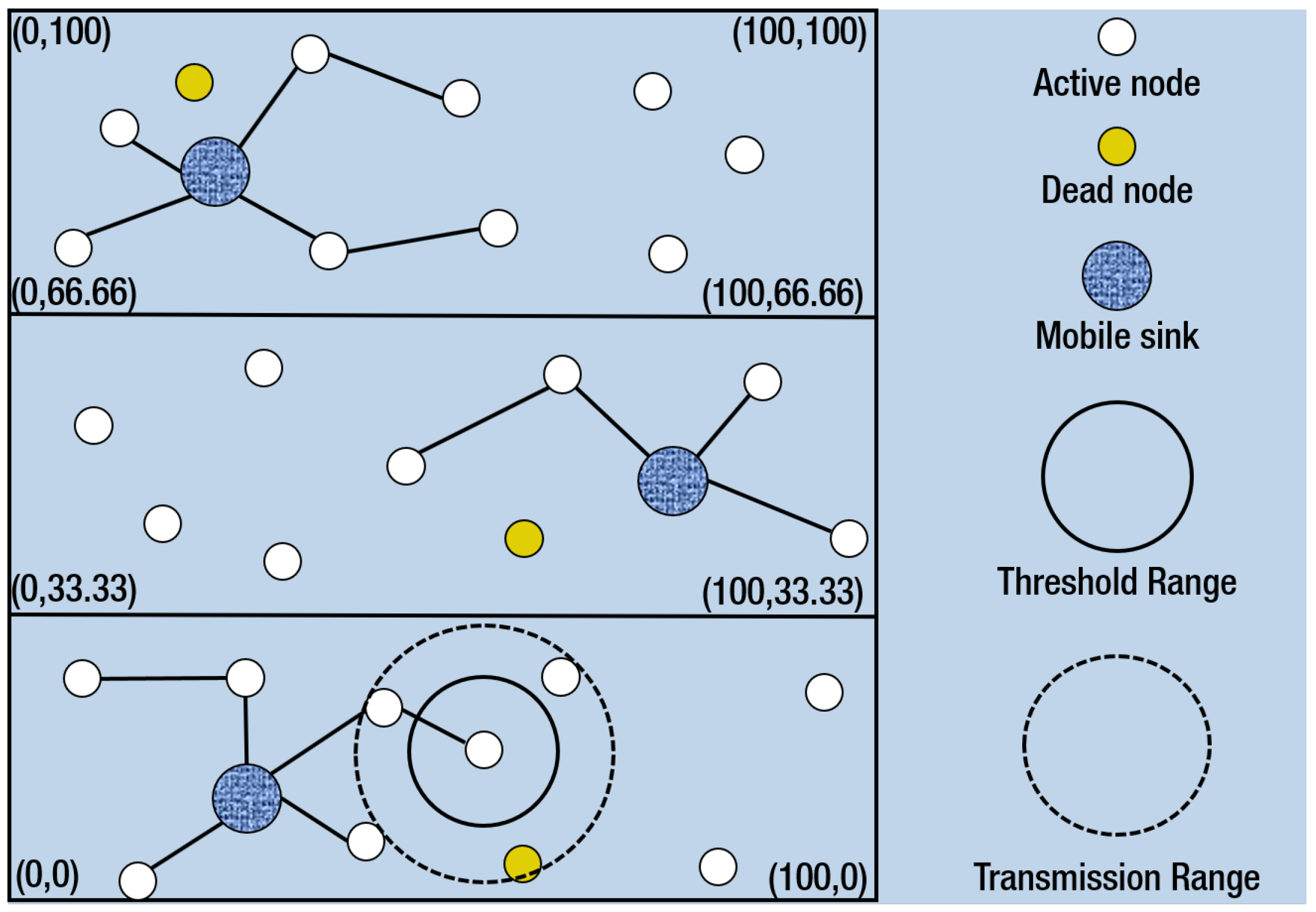
3.7.1. Regional Sink Mobility (RSM)

In RSM the whole region is divided into three equal parts which is depicted in Figure 12. All the nodes in the network are placed arbitrarily in these three regions. Three Mobile sink are deployed in three different regions. They move randomly in each round within their own region. When sink 1 moves and takes a new position, the position of the sink two must be such that it maintains maximum distance from the sink 1. Similarly sink 3 must maintain the maximum distance based on the new position of the sink 2. This condition is applied to get a larger coverage area.
The sensor nodes lying in regions one and two transmit the data to sink one or two. Similarly sink two or three collect the data from the area two and three. if the sensor nodes fall within the range of the designated sink then it directly delivers the data to the sink. But if any node falls out of the range of the sink then it chooses another suitable node through which it can send its data to the sink. When a node falls out of the threshold range but remains within the transmission range then it is considered as a neighbor of the sender. Now if a neighboring node of the sender is in the range of the sink one or sink two, can be declared as eligible neighbor for receiving. Then the sender node transmit the data packet to the neighboring node and from that node mobile sink gets the data. If a node neither finds any sink within its threshold nor finds an eligible neighboring node then data of this node is discarded.

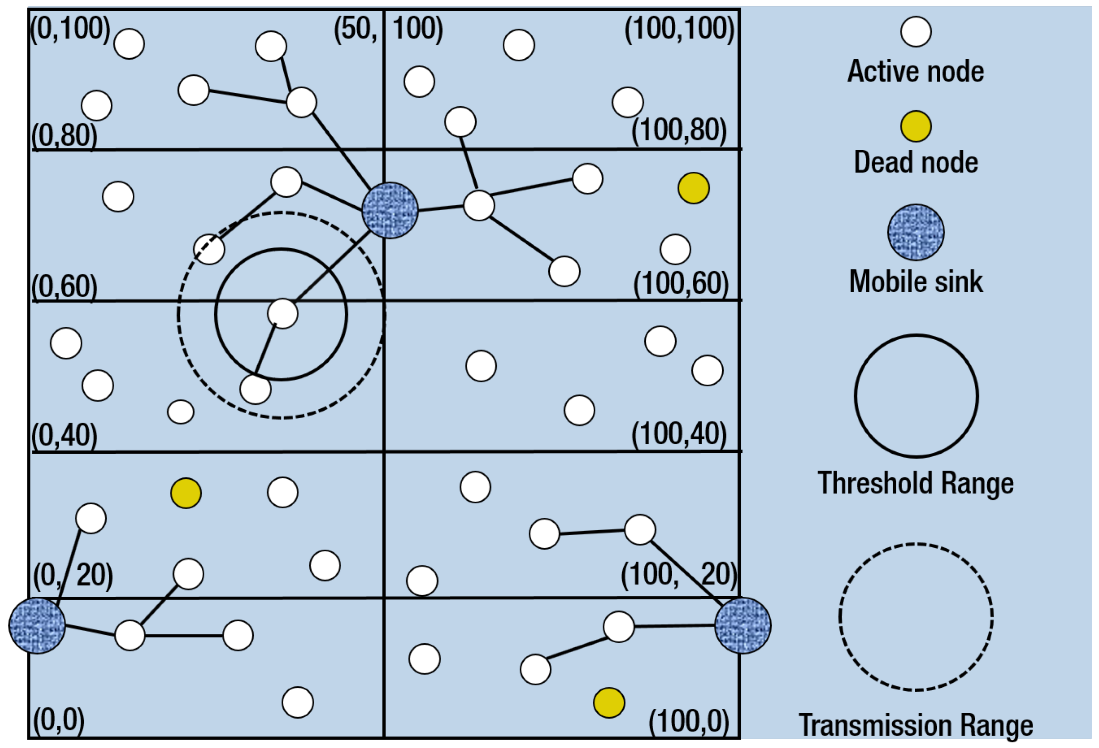
3.7.2. Vertical Sink Mobility (VSM)

Data transmission of VSM is depicted by Figure 13 which shows that the whole network area is divided into 10 equal parts. Sensor nodes are placed arbitrarily over the whole volume. Three mobile sinks are employed for the whole volume of the area with a predefined distance from each other to maximize the coverage area. These sinks take a new position in every round in such a way that they maintain this predefined distance from each other. When one round ends sink one take a new position by traveling a preset distance in X or Y axis. Sink two traverse the same distance in same direction of the same coordinate to maintain that predefined distance. Similarly Sink three take position depending on the position of the sink two. To transmit data packet, every node calculates its distance with the sink and neighboring nodes. If it finds one or more sinks within its transmission range, the node directly transmit to the sink. If all of the sinks are out of the range, the sending node tries to find a neighboring node who has a sink within its range. In this case, the neighboring node transmit the received data from sending node to the sink. But unfortunately, if there is no eligible neighboring nodes even, then the data packet has to be discarded.
Both RSM and VSM either transmit directly or by two hop transmission method to the sink. This improves the throughput, the data received rate and initial network stability of both the schemes and have better performance than SEEC. Throughput of VSM is twice and that of RSM is thrice of the throughput of SEEC. But these two schemes possess some limitations also. In both the schemes every node take part in transmission, which eventually decrease the residual energy. So the energy of the nodes decrease fast causing their death. Death of the nodes results in a network hole disrupting the network stability. Stability of SEEC is not that prominent at the beginning compared to RSM and VSM but after 800 rounds, SEEC shows more stability than RSM and VSM. The low residual energy causes the death of the nodes earlier which affects the network lifetime of both RSM and VSM. SEEC has longer network lifetime than these two schemes. Even though RSM and VSM gives high performance in throughput and data received rate, their network stability and network lifetime is less than that of SEEC.

4. Evaluation of the Routing Protocols

Different types of design philosophies and application requirements have to be considered in most of the routing schemes proposed for UWSN. None of these protocols work efficiently for every parameter such as localization, reliability, node mobility, network life-time, latency and energy-efficiency. Every protocol has its own edge and also few drawbacks. An overview of the key features and drawbacks of the considered routing protocols are depicted in Table 3.
For evaluating the performance of both the terrestrial and underwater sensor networks, the most frequently used techniques are: (i) analytical modeling, (ii) real deployment, and (iii) numerical simulation.
For UWSN protocols most researchers evaluate their scheme with analytical modeling and numerical simulation. The most commonly used simulation tool is NS-2. Table 4 presents the detailed comparison of the routing protocols considering delivery ratio, energy-efficiency, delay-efficiency, localization requirement, reliability and overall performance.
Different routing protocols are suitable for different conditions considering different parameters like network size, localization, reliability and node mobility. There is no routing protocol which gives most efficient performance in every scenario. EBER2, CoDBR, RE-PBR, VTP give best performance in terms of delivery ratio whereas EBER2 and SEEC are most energy efficient. The delay efficiency of RE-PBR and VTP is better than any other considered routing protocols. On the other hand, EBER2, CoDBR and RE-PBR offer highest reliability in data transmission in compared to others. Considering all the metrics and factors, the overall performances of EBER2 and RE-PBR are better than any other considered routing protocols for UWSN.
Even though UWSN has improved a lot due to massive efforts from researchers, it still possesses several challenges which include time synchronization, localization accuracy, wave speed variation and security issues. Most of these challenges are not addressed in the above-discussed routing protocols and these are open research issues. Time synchronization is one of the important factors for localization [42]. The sink nodes floating at the water surface can synchronize their time from GPS data whereas the underwater nodes face problem in time-synchronization due to clock skew and offsets [73]. Most of the routing protocols described here do not consider the speed variation of the acoustic waves due salinity, water pressure and temperature. This might cause discrepancies in distance measurement which affects the the localization and routing decisions [73]. Security in UWSN is one of the very important issues that has to be considered for practical deployment [74]. Countermeasures against security attacks needs to be considered while designing the routing protocols and this challenge is still open for research.

5. Conclusions

A detailed evaluation and survey of the latest advanced routing schemes for UWSN are performed in this paper. The nature of underwater acoustic communication and the network architectures in regards to reliability, latency, energy-efficiency and localization are described elaborately. Moreover, using these primary factors as metrics, some overviews of significant routing protocols of UWSN are discussed. In UWSN, due to multiple issues—for example, limitation of energy, harsh environment, difficult localization, path loss, low data rate, and so forth—the design of routing protocols is challenging and has become a vital research area due to its enormous applications and opportunities. Each of the considered routing protocols shows the robustness and the weakness depending on the underwater networking environment and scenarios. Different protocols are suitable for different situations and functions depending on the priority of the demands and deploying environment. Considering all the factors, EBER2 and RE-PBR showed better overall performances compared to other considered routing protocols discussed in this paper.
This survey summarizes the remaining challenging issues and the future trends of some of the advanced routing protocols. This work encourages further research efforts to improve the routing protocols of UWSN for enhanced underwater monitoring and exploration. Future work will involve further exploring routing protocols and localization to improve on these challenges and to propose a more reliable and efficient but also flexible routing protocol.

Author Contributions

K.F.H. planned and performed the survey. He analyzed, produced the initial manuscript and edited till the final submission. K.H.K. conceived the idea and continuously supervised and revised the manuscript for improvement. And, A.A. supervised and gave necessary enhancements and inputs along with the work. All authors have read and agreed to the published version of the manuscript.

Funding

This research is funded by School of Engineering and Technology and Faculty Research and Creative Endeavors (FRCE) of Central Michigan University, MI, USA

Conflicts of Interest

The authors declare no conflict of interest.

References

  1. Immas, A.; Saadat, M.; Navarro, J.; Drake, M.; Shen, J.; Alam, M.R. High-bandwidth underwater wireless communication using a swarm of autonomous underwater vehicles. In Proceedings of the ASME 2019 38th International Conference on Ocean, Offshore and Arctic Engineering, Glasgow, UK, 9–14 June 2019; American Society of Mechanical Engineers Digital Collection: New York, NY, USA. [Google Scholar]
  2. Akyildiz, I.F.; Pompili, D.; Melodia, T. Underwater acoustic sensor networks: Research challenges. Ad Hoc Netw. 2005, 3, 257–279. [Google Scholar] [CrossRef]
  3. Heidemann, J.; Ye, W.; Wills, J.; Syed, A.; Li, Y. Research challenges and applications for underwater sensor networking. In Proceedings of the IEEE Wireless Communications and Networking Conference, WCNC 2006, Las Vegas, NV, USA, 3–6 April 2006; IEEE: Piscataway, NJ, USA, 2006; Volume 1, pp. 228–235. [Google Scholar]
  4. Goyal, N.; Dave, M.; Verma, A.K. Protocol stack of underwater wireless sensor network: Classical approaches and new trends. Wirel. Pers. Commun. 2019, 104, 995–1022. [Google Scholar] [CrossRef]
  5. Li, S.; Qu, W.; Liu, C.; Qiu, T.; Zhao, Z. Survey on high reliability wireless communication for underwater sensor networks. J. Netw. Comput. Appl. 2019, 148, 102446. [Google Scholar] [CrossRef]
  6. Sun, Y.; Yuan, Y.; Xu, Q.; Hua, C.; Guan, X. A Mobile Anchor Node Assisted RSSI Localization Scheme in Underwater Wireless Sensor Networks. Sensors 2019, 19, 4369. [Google Scholar] [CrossRef] [PubMed] [Green Version]
  7. Yan, J.; Xu, Z.; Wan, Y.; Chen, C.; Luo, X. Consensus estimation-based target localization in underwater acoustic sensor networks. Int. J. Robust Nonlinear Control 2017, 27, 1607–1627. [Google Scholar] [CrossRef]
  8. Murad, M.; Sheikh, A.A.; Manzoor, M.A.; Felemban, E.; Qaisar, S. A Survey on Current Underwater Acoustic Sensor Network Applications. Int. J. Comput. Theory Eng. 2015, 7, 51. [Google Scholar] [CrossRef] [Green Version]
  9. Kumar, P.; Kumar, P.; Priyadarshini, P. Underwater acoustic sensor network for early warning generation. In Proceedings of the 2012 Oceans, Hampton Roads, VA, USA, 14–19 October 2012; IEEE: Piscataway, NJ, USA, 2012; pp. 1–6. [Google Scholar]
  10. Casey, K.; Lim, A.; Dozier, G. A sensor network architecture for tsunami detection and response. Int. J. Distrib. Sens. Netw. 2008, 4, 27–42. [Google Scholar] [CrossRef] [Green Version]
  11. Handziski, V.; Koepke, A.; Karl, H.; Frank, C.; Drytkiewicz, W. Improving the energy efficiency of directed diffusion using passive clustering. In Proceedings of the European Workshop on Wireless Sensor Networks, Berlin, Germany, 19–21 January 2004; Springer: Berlin/Heidelberg, Germany, 2004; pp. 172–187. [Google Scholar]
  12. Felemban, E.; Shaikh, F.K.; Qureshi, U.M.; Sheikh, A.A.; Qaisar, S.B. Underwater sensor network applications: A comprehensive survey. Int. J. Distrib. Sens. Netw. 2015, 2015, 5. [Google Scholar] [CrossRef] [Green Version]
  13. Thornton, B.; Bodenmann, A.; Asada, A.; Sato, T.; Ura, T. Acoustic and visual instrumentation for survey of manganese crusts using an underwater vehicle. In Proceedings of the 2012 Oceans, Hampton Roads, VA, USA, 14–19 October 2012; IEEE: Piscataway, NJ, USA, 2012; pp. 1–10. [Google Scholar]
  14. Srinivas, S.; Ranjitha, P.; Ramya, R.; Narendra, G.K. Investigation of oceanic environment using large-scale uwsn and uanets. In Proceedings of the 2012 8th International Conference on Wireless Communications, Networking and Mobile Computing (WiCOM), Shanghai, China, 21–23 September 2012; pp. 1–5. [Google Scholar]
  15. Khan, A.; Jenkins, L. Undersea wireless sensor network for ocean pollution prevention. In Proceedings of the 2008 3rd International Conference on Communication Systems Software and Middleware and Workshops (COMSWARE’08), Bangalore, India, 6–10 January 2008; IEEE: Piscataway, NJ, USA, 2008; pp. 2–8. [Google Scholar]
  16. Du, X.; Liu, X.; Su, Y. Underwater acoustic networks testbed for ecological monitoring of Qinghai Lake. In Proceedings of the OCEANS 2016, Shanghai, China, 10–13 April 2016; IEEE: Piscataway, NJ, USA, 2016; pp. 1–4. [Google Scholar]
  17. Lloret, J.; Sendra, S.; Garcia, M.; Lloret, G. Group-based underwater wireless sensor network for marine fish farms. In Proceedings of the 2011 IEEE GLOBECOM Workshops (GC Wkshps), Houston, TX, USA, 5–9 December 2011; IEEE: Piscataway, NJ, USA, 2011; pp. 115–119. [Google Scholar]
  18. Mohamed, N.; Jawhar, I.; Al-Jaroodi, J.; Zhang, L. Sensor network architectures for monitoring underwater pipelines. Sensors 2011, 11, 10738–10764. [Google Scholar] [CrossRef] [Green Version]
  19. Henry, N.F.; Henry, O.N. Wireless sensor networks based pipeline vandalisation and oil spillage monitoring and detection: Main benefits for nigeria oil and gas sectors. SIJ Trans. Comput. Sci. Eng. Its Appl. (CSEA) 2015, 3, 1–6. [Google Scholar]
  20. Allen, C. Wireless sensor network nodes: Security and deployment in the niger-delta oil and gas sector. Int. J. Netw. Security & Its Appl. (IJNSA) 2011, 3, 68–79. [Google Scholar]
  21. Freitag, L.; Grund, M.; Von Alt, C.; Stokey, R.; Austin, T. A shallow water acoustic network for mine countermeasures operations with autonomous underwater vehicles. In Proceedings of the Underwater Defense Technology (UDT), Amsterdam, The Netherlands, 21–23 June 2005; pp. 1–6. [Google Scholar]
  22. Jouhari, M.; Ibrahimi, K.; Tembine, H.; Ben-Othman, J. Underwater wireless sensor networks: A survey on enabling technologies, localization protocols, and internet of underwater things. IEEE Access 2019, 7, 96879–96899. [Google Scholar] [CrossRef]
  23. Khan, A.; Ahmedy, I.; Anisi, M.H.; Javaid, N.; Ali, I.; Khan, N.; Alsaqer, M.; Mahmood, H. A localization-free interference and energy holes minimization routing for underwater wireless sensor networks. Sensors 2018, 18, 165. [Google Scholar] [CrossRef] [PubMed] [Green Version]
  24. Ayaz, M.; Baig, I.; Abdullah, A.; Faye, I. A survey on routing techniques in underwater wireless sensor networks. J. Netw. Comput. Appl. 2011, 34, 1908–1927. [Google Scholar] [CrossRef]
  25. Kremer, K. Advanced underwater technology with emphasis on acoustic modeling and systems. Hydroacoustics 1997, 1. [Google Scholar] [CrossRef] [Green Version]
  26. Stojanovic, M. Acoustic (underwater) communications. In Encyclopedia of Telecommunications; John Wiley & Sons, Inc.: Hoboken, NJ, USA, 2003. [Google Scholar]
  27. Li, B.; Huang, J.; Zhou, S.; Ball, K.; Stojanovic, M.; Freitag, L.; Willett, P. MIMO-OFDM for high-rate underwater acoustic communications. IEEE J. Ocean. Eng. 2009, 34, 634–644. [Google Scholar]
  28. Amruta, M.K.; Satish, M.T. Solar powered water quality monitoring system using wireless sensor network. In Proceedings of the 2013 International Mutli-Conference on Automation, Computing, Communication, Control and Compressed Sensing (iMac4s), Kottayam, India, 22–23 March 2013; IEEE: Piscataway, NJ, USA; pp. 281–285. [Google Scholar]
  29. Pule, M.; Yahya, A.; Chuma, J. Wireless sensor networks: A survey on monitoring water quality. J. Appl. Res. Technol. 2017, 15, 562–570. [Google Scholar] [CrossRef]
  30. Jin, N.; Ma, R.; Lv, Y.; Lou, X.; Wei, Q. A novel design of water environment monitoring system based on wsn. In Proceedings of the 2010 International Conference on Computer Design and Applications, Qinhuangdao, China, 25–27 June 2010; IEEE: Piscataway, NJ, USA; Volume 2, pp. V2–V593. [Google Scholar]
  31. Verma, S. Wireless Sensor Network application for water quality monitoring in India. In Proceedings of the 2012 National Conference on Computing and Communication Systems, Durgapur, India, 21–22 November 2012; IEEE: Piscataway, NJ, USA; pp. 1–5. [Google Scholar]
  32. Shi, B.; Sreeram, V.; Zhao, D.; Duan, S.; Jiang, J. A wireless sensor network-based monitoring system for freshwater fishpond aquaculture. Biosyst. Eng. 2018, 172, 57–66. [Google Scholar] [CrossRef]
  33. Hiremath, V. Design and development of wireless sensor network system to monitor parameters influencing freshwater fishes. Int. J. Comput. Sci. Eng. 2012, 4, 1096. [Google Scholar]
  34. Sutar, K.G.; Patil, R.T. Wireless sensor network system to monitor the fish farm. Int. J. Eng. Res. Appl. 2013, 3, 194–197. [Google Scholar]
  35. Abdulameer, D.N.; Ahmad, R. Underwater Acoustic Communications Using Direct-Sequence Spread Spectrum. Int. J. Comput. Sci. Issues (IJCSI) 2014, 11, 76. [Google Scholar]
  36. Akyildiz, I.F.; Pompili, D.; Melodia, T. State-of-the-art in protocol research for underwater acoustic sensor networks. In Proceedings of the 1st ACM International Workshop on Underwater Networks, Los Angeles, CA, USA, September 2006; ACM: New York, NY, USA, 2006; pp. 7–16. [Google Scholar]
  37. Cañete, F.J.; López-Fernández, J.; García-Corrales, C.; Sánchez, A.; Robles, E.; Rodrigo, F.J.; Paris, J.F. Measurement and modeling of narrowband channels for ultrasonic underwater communications. Sensors 2016, 16, 256. [Google Scholar] [CrossRef] [PubMed]
  38. Xie, P.; Cui, J.H.; Lao, L. VBF: Vector-based forwarding protocol for underwater sensor networks. In Proceedings of the International Conference on Research in Networking, Coimbra, Portugal, 15–19 May 2006; Springer: Berlin/Heidelberg, Germany; pp. 1216–1221. [Google Scholar]
  39. Beniwal, M.; Singh, R.P.; Sangwan, A. A localization scheme for underwater sensor networks without Time Synchronization. Wirel. Pers. Commun. 2016, 88, 537–552. [Google Scholar] [CrossRef]
  40. Luo, J.; Fan, L.; Wu, S.; Yan, X. Research on localization algorithms based on acoustic communication for underwater sensor networks. Sensors 2018, 18, 67. [Google Scholar] [CrossRef] [Green Version]
  41. Ahmed, M.; Salleh, M. Localization schemes in underwater sensor network (UWSN): A survey. Indones. J. Electr. Eng. Comput. Sci. 2016, 1, 119–125. [Google Scholar] [CrossRef]
  42. Su, X.; Ullah, I.; Liu, X.; Choi, D. A Review of Underwater Localization Techniques, Algorithms, and Challenges. J. Sensors 2020, 2020, 6403161. [Google Scholar] [CrossRef]
  43. Erol, M.; Vieira, L.F.; Gerla, M. Localization with Dive’N’Rise (DNR) beacons for underwater acoustic sensor networks. In Proceedings of the Second Workshop on Underwater Networks, Montreal, QC, Canada, September 2007; ACM: New York, NY, USA; pp. 97–100. [Google Scholar]
  44. Chen, K.; Zhou, Y.; He, J. A localization scheme for underwater wireless sensor networks. Int. J. Adv. Sci. Technol. 2009, 4, 9–16. [Google Scholar]
  45. Ayaz, M.; Jung, L.T.; Abdullah, A.; Ahmad, I. Reliable data deliveries using packet optimization in multi-hop underwater sensor networks. J. King Saud Univ.-Comput. Inf. Sci. 2012, 24, 41–48. [Google Scholar] [CrossRef] [Green Version]
  46. Khan, A.; Ali, I.; Ghani, A.; Khan, N.; Alsaqer, M.; Rahman, A.U.; Mahmood, H. Routing protocols for underwater wireless sensor networks: Taxonomy, research challenges, routing strategies and future directions. Sensors 2018, 18, 1619. [Google Scholar] [CrossRef] [Green Version]
  47. Xiao, Y. Underwater Scoustic Sensor Networks; CRC Press: Boca Raton, FL, USA, 2010. [Google Scholar]
  48. Mackenzie, K.V. Nine-term equation for sound speed in the oceans. J. Acoust. Soc. Am. 1981, 70, 807–812. [Google Scholar] [CrossRef]
  49. Khalid, M.; Ullah, Z.; Ahmad, N.; Arshad, M.; Jan, B.; Cao, Y.; Adnan, A. A survey of routing issues and associated protocols in underwater wireless sensor networks. J. Sensors 2017, 2017, 7539751. [Google Scholar] [CrossRef]
  50. Islam, T.; Lee, Y.K. A Comprehensive Survey of Recent Routing Protocols for Underwater Acoustic Sensor Networks. Sensors 2019, 19, 4256. [Google Scholar] [CrossRef] [PubMed] [Green Version]
  51. Nicolaou, N.; See, A.; Xie, P.; Cui, J.H.; Maggiorini, D. Improving the robustness of location-based routing for underwater sensor networks. In Proceedings of the OCEANS 2007-Europe, Aberdeen, UK, 18–21 June 2007; IEEE: Piscataway, NJ, USA, 2007; pp. 1–6. [Google Scholar]
  52. Yan, H.; Shi, Z.J.; Cui, J.H. DBR: Depth-based routing for underwater sensor networks. In Proceedings of the International Conference on Research in Networking, Singapore, 5–9 May 2008; Springer: Berlin/Heidelberg, Germany; pp. 72–86. [Google Scholar]
  53. Bharathy, A.V.; Chandrasekar, V. A Novel Virtual Tunneling Protocol for Underwater Wireless Sensor Networks. In Soft Computing and Signal Processing; Springer: Berlin/Heidelberg, Germany, 2019; pp. 281–289. [Google Scholar]
  54. Nasir, H.; Javaid, N.; Ashraf, H.; Manzoor, S.; Khan, Z.A.; Qasim, U.; Sher, M. CoDBR: Cooperative depth based routing for underwater wireless sensor networks. In Proceedings of the 2014 Ninth International Conference on Broadband and Wireless Computing, Communication and Applications, Guangdong, China, 8–10 November 2014; IEEE: Piscataway, NJ, USA, 2014; pp. 52–57. [Google Scholar]
  55. Wahid, A.; Lee, S.; Jeong, H.J.; Kim, D. Eedbr: Energy-efficient depth-based routing protocol for underwater wireless sensor networks. In Advanced Computer Science and Information Technology; Springer: Berlin/Heidelberg, Germany, 2011; pp. 223–234. [Google Scholar]
  56. Khasawneh, A.; Latiff, M.S.B.A.; Kaiwartya, O.; Chizari, H. A reliable energy-efficient pressure-based routing protocol for underwater wireless sensor network. Wirel. Netw. 2018, 24, 2061–2075. [Google Scholar] [CrossRef]
  57. Shin, D.; Hwang, D.; Kim, D. DFR: An efficient directional flooding-based routing protocol in underwater sensor networks. Wirel. Commun. Mob. Comput. 2012, 12, 1517–1527. [Google Scholar] [CrossRef]
  58. Shen, J.; Tan, H.W.; Wang, J.; Wang, J.W.; Lee, S.Y. A novel routing protocol providing good transmission reliability in underwater sensor networks. J. Internet Technol. 2015, 16, 171–178. [Google Scholar]
  59. Jornet, J.M.; Stojanovic, M.; Zorzi, M. Focused beam routing protocol for underwater acoustic networks. In Proceedings of the Third ACM International Workshop on Underwater Networks, San Francisco, CA, USA, September 2008; ACM: New York, NY, USA; pp. 75–82. [Google Scholar]
  60. Domingo, M.C.; Prior, R. A distributed clustering scheme for underwater wireless sensor networks. In Proceedings of the 2007 IEEE 18th International Symposium on Personal, Indoor and Mobile Radio Communications, Athens, Greece, 3–7 September 2007; IEEE: Piscataway, NJ, USA, 2007; pp. 1–5. [Google Scholar]
  61. Azam, I.; Majid, A.; Ahmad, I.; Shakeel, U.; Maqsood, H.; Khan, Z.A.; Qasim, U.; Javaid, N. SEEC: Sparsity-aware energy efficient clustering protocol for underwater wireless sensor networks. In Proceedings of the 2016 IEEE 30th International Conference on Advanced Information Networking and Applications (AINA), Crans-Montana, Switzerland, 23–25 March 2016; IEEE: Piscataway, NJ, USA, 2016; pp. 352–361. [Google Scholar]
  62. Guangzhong, L.; Zhibin, L. Depth-based multi-hop routing protocol for underwater sensor network. In Proceedings of the 2010 The 2nd International Conference on Industrial Mechatronics and Automation (ICIMA), Wuhan, China, 30–31 May 2010; Volume 2, pp. 268–270. [Google Scholar]
  63. Wadud, Z.; Ismail, M.; Qazi, A.B.; Khan, F.A.; Derhab, A.; Ahmad, I.; Ahmad, A.M. An Energy Balanced Efficient and Reliable Routing Protocol for Underwater Wireless Sensor Networks. IEEE Access 2019, 7, 175980–175999. [Google Scholar] [CrossRef]
  64. Ali, B.; Javaid, N.; Islam, S.U.; Ahmed, G.; Qasim, U.; Khan, Z.A. RSM and VSM: Two New Routing Protocols for Underwater WSNs. In Proceedings of the 2016 International Conference on Intelligent Networking and Collaborative Systems (INCoS), Ostrawva, Czech Republic, 7–9 September 2016; IEEE: Piscataway, NJ, USA, 2016; pp. 173–179. [Google Scholar]
  65. Yu, H.; Yao, N.; Wang, T.; Li, G.; Gao, Z.; Tan, G. WDFAD-DBR: Weighting depth and forwarding area division DBR routing protocol for UASNs. Ad Hoc Netw. 2016, 37, 256–282. [Google Scholar] [CrossRef]
  66. Hu, T.; Fei, Y. MURAO: A multi-level routing protocol for acoustic-optical hybrid underwater wireless sensor networks. In Proceedings of the 2012 9th Annual IEEE Communications Society Conference on Sensor, Mesh and Ad Hoc Communications and Networks (SECON), Seoul, South Korea, 18–21 June 2012; IEEE: Piscataway, NJ, USA, 2012; pp. 218–226. [Google Scholar]
  67. Basagni, S.; Petrioli, C.; Petroccia, R.; Spaccini, D. CARP: A channel-aware routing protocol for underwater acoustic wireless networks. Ad Hoc Netw. 2015, 34, 92–104. [Google Scholar] [CrossRef]
  68. Noh, Y.; Lee, U.; Wang, P.; Choi, B.S.C.; Gerla, M. VAPR: Void-aware pressure routing for underwater sensor networks. IEEE Trans. Mob. Comput. 2013, 12, 895–908. [Google Scholar] [CrossRef]
  69. Hussain, S.N.; Hussain, M.M.; Aslam, M.G. Flooding based routing techniques for efficient communication in underwater wsns1. Eur. J. Comput. Sci. Inf. Technol. 2015, 3, 52–60. [Google Scholar]
  70. De Morais Cordeiro, C.; Agrawal, D.P. Ad Hoc and Sensor Networks: Theory and Applications; World Scientific: Singapore, 2011. [Google Scholar]
  71. Zhangjie, F.; Xingming, S.; Qi, L.; Lu, Z.; Jiangang, S. Achieving efficient cloud search services: Multi-keyword ranked search over encrypted cloud data supporting parallel computing. IEICE Trans. Commun. 2015, 98, 190–200. [Google Scholar]
  72. Jornet, J.M.; Stojanovic, M. Distributed power control for underwater acoustic networks. In Proceedings of the OCEANS 2008, Quebec City, QC, Canada, 15–18 September 2008; IEEE: Piscataway, NJ, USA, 2008; pp. 1–7. [Google Scholar]
  73. Hu, K.; Song, X.; Sun, Z.; Luo, H.; Guo, Z. Localization based on map and pso for drifting-restricted underwater acoustic sensor networks. Sensors 2019, 19, 71. [Google Scholar] [CrossRef] [PubMed] [Green Version]
  74. Li, H.; He, Y.; Cheng, X.; Zhu, H.; Sun, L. Security and privacy in localization for underwater sensor networks. IEEE Commun. Mag. 2015, 53, 56–62. [Google Scholar] [CrossRef]
Figure 1. Underwater Pipeline Monitoring with UWSN.
Jsan 09 00019 g001
Figure 2. Two dimensional (2D) UWSN architecture.
Jsan 09 00019 g002
Figure 3. Routing Procedure of Vector Based Forwarding (VBF) [38].
Jsan 09 00019 g003
Figure 4. Routing Technique of Depth Based Routing (DBR) [52].
Jsan 09 00019 g004
Figure 5. Data transmission in Cooperative Depth Based Routing (CoDBR) [54].
Jsan 09 00019 g005
Figure 6. Data transmission in Virtual Tunneling Protocol (VTP) [53].
Jsan 09 00019 g006
Figure 7. Network architecture in Reliable Energy Efficient Pressure Based Routing (RE-PBR) [56].
Jsan 09 00019 g007
Figure 8. Packet transmission in Directional Flooding-Based Routing (DFR) [57].
Jsan 09 00019 g008
Figure 9. Data transmission in Location-Aware Routing Protocol (LARP) [58].
Jsan 09 00019 g009
Figure 10. Data Forwarding Techniques in Focused Beam Routing (FBR) [59].
Jsan 09 00019 g010
Figure 11. Network architecture of Energy Balanced Efficient and Reliable Routing Protocol (EBER2) [63].
Jsan 09 00019 g011
Figure 12. Data transmission in Regional Sink Mobility (RSM) [64].
Jsan 09 00019 g012
Figure 13. Data transmission in Vertical Sink Mobility (VSM) [64].
Jsan 09 00019 g013
Table 1. Acoustic Channels of UWSN in terms of operating frequency band, bandwidth, direct transmission range, and applications [2,25,26].
Operating Frequency Bands (kHz)Direct Transmission Range with no hopping (km)Bandwidth (kHz)Applications
0.01–11000
(Very Long)
<1
(Very Low)
For Very Long Range and Very Low Bandwidth Applications:
Ocean Monitoring, Marine Life Monitoring [15,16,17].
1–510–100
(Long)
2–5
(Low)
For Long Range and Low Bandwidth Applications:
Underwater Pipeline Monitoring and Natural Hazard Detection [8,9,10,11,18,19,20].
5–101–10
(Medium)
≈10
(Medium)
For Medium Range and Medium Bandwidth Applications:
Underwater Mapping, Locating Mineral Mines and Military Applications [2,13,14,21].
10–1000.1–1
(Short)
20–50
(High)
For Short Range and High Bandwidth Applications:
Lake / River Water Quality monitoring [28,29,30,31].
100–1000<1
(Very Short)
>100
(Very High)
For Very Short Range and Very High Bandwidth Applications:
Fresh Water Fish Farm [32,33,34].
Table 2. Classification of Routing Protocols.
Sl. No.Name of the Routing ProtocolsFeature Based ClassificationClassification Based on Localization
1Vector Based Forwarding (VBF) [38]Node MobilityLocation Based
2Hop-by-Hop VBF (HH-VBF) [51]Node MobilityLocation Based
3Depth Based Routing (DBR) [52]Node MobilityLocation Free
4Virtual Tunneling Protocol (VTP) [53]Node MobilityLocation Free
5Cooperative Depth Based Routing (CoDBR) [54]Node MobilityLocation Free
6Energy-Efficient DBR (EEDBR) [55]Energy BalancingLocation Free
7Reliable Energy Efficient Pressure Based Routing (RE-PBR) [56]Energy BalancingLocation Free
8Directional Flooding-Based Routing (DFR) [57]Channel PropertiesLocation Based
9Location-Aware Routing Protocol (LARP) [58]Channel PropertiesLocation Based
10Focused beam routing (FBR) [59]Energy EfficiencyLocation Based
11Distributed Underwater Clustering Scheme (DUCS) [60]Energy EfficiencyLocation Free
12Sparsity-aware Energy Efficient Clustering Protocol (SEEC) [61]Energy EfficiencyLocation Free
13Depth Based Multi-Hop Routing (DMBR) [62]Energy EfficiencyLocation Free
14An Energy Balanced Efficient and Reliable Routing Protocol (EBER2) [63]Network Void Hole AvoidanceLocation Free
15Regional Sink Mobility (RSM) [64]Network Void Hole AvoidanceLocation Free
16Vertical sink Mobility (VSM) [64]Network Void Hole AvoidanceLocation Free
17Weighting Depth and Forwarding Area Division DBR (WDFAD-DBR) [65]Network Void Hole AvoidanceLocation Free
Table 3. Key features and main drawbacks of different routing protocols.
Sl. No.Name of the ProtocolsKey FeaturesMain Drawbacks
1Vector Based Forwarding (VBF) [38]1. End-to-End forwarding.
2. Location based scheme.
3. Only few nodes take part in routing where others sit idle.
4. Doesn’t require any state information.
5. Scalable to the network demand.
6. Energy efficient.
7. In dense network gives descent performance.
1. In sparse network packet delivery rate degraded drastically.
2. Difficult to find proper routing radius threshold.
2Hop-by-Hop VBF (HH-VBF) [51]1. The data transmission is done by ho-by-hop technique.
2. In Sparse region, it gives better packet delivery ratio than VBF.
1. Gives more signal overhead than VBF.
3Depth Based Routing (DBR) [52]1. Packet forwarding decision by a node is taken depending on its depth and the prior sender.
2. Only the depth information of the node is necessary.
3. Gives good performance in dense network.
1. It works only in greedy mode.
2. Packet delivery ratio degrades in sparse network.
4Virtual Tunneling Protocol (VTP) [53]1. It is a cluster based scheme.
2. It forms a virtual tunnel for a strong connection from source to the destination.
3. Three-way handshake is followed for packet data transfer.
4. It gives better packet delivery rate, latency in compared to CARP and MURAO.
1. It might not be an energy efficient scheme as it follows three-way handshake to transfer single data packet.
5Cooperative DBR (CoDBR) [54]1. DBR is incorporated with path diversity via multiple path to increase reliability.
2. Localization free protocol.
3. Next hop is selected based on the nodes having minimum depth.
4. Unlike DBR simultaneously same data is transmitted twice.
5. Data packet is dropped if it crosses the maximum allowable bit error rate.
6. It has higher reliability than DBR but it’s energy consumption is also higher than DBR.
7. It offers 83% more throughput and and 90% less packet drop.
1. Energy consumption is higher than DBR.
2. Network life is shorter than DBR.
6Reliable and Energy efficient PBR (RE-PBR) [56]1. Depth based and localization free protocol.
2. It measures link quality precisely with triangle metric.
3. Next forwarding node is selected basing on residual energy and triangle metric based link quality.
4. Its network lifetime is longer than DBR and EEDBR.
5. Comparing it to the DBR and EEDBR it gives better delivery ratio.
6. It consumes less energy than DBR and EEDBR but provides higher reliability than these two protocol.
1. As the node increases, energy consumption increases in compared to DBR and EEDBR.
7Directional Flooding-Based Routing (DFR) [57]1. Per hop forwarding is followed.
2. Comparing BASE ANGLE with CURRENT ANGLE a node decides whether to forward the data.
3. It gives better delivery ratio than VBF.
4. Shorter end-to-end delay and less communication overhead than VBF.
1. Network is disrupted when a hole is created due to absence of any node near to the sink.
8Location-Aware Routing Protocol (LARP) [58]1. Good packet delivery ratio.
2. To know the nodes’ location it uses a technique called RSSI.
3. Provides more reliable transmission than other routing protocols.
1. To work perfectly it needs very dense network.
2. It has low delay efficiency.
9Focused Beam Routing (FBR) [59]1. Avoids Unnecessary flooding.
2. It works well with both the steady and moving nodes.
3. A source node has to know only its position and position of the destination.
4. It reduces energy consumption by maintaining different power levels.
1. This scheme increases the overhead.
2. Network is more restricted as the sink is fixed.
10Distributed Underwater Clustering Scheme (DUCS) [60]1. It is a self changeable routing protocol which can assemble itself.
2. Distributed algorithm is used to form the clusters.
3. Intra-cluster Communications and inter-cluster communications are controlled by cluster head.
4. Random rotation of cluster head.
5. Energy efficient.
6. Increased throughput.
1. Water current may reduce cluster life by affecting its structure.
2. Inter-cluster communications depend solely on cluster head.
11Sparsity-aware energy efficient clustering protocol (SEEC) [61]1. SEEC is location free routing scheme which features the energy efficiency
2. The whole deployed region is divided into few regions and dense and sparse regions are sorted out.
3. UW-Sinks collect the data from the sparse region whereas clustering scheme is applied in dense network regions.
4. It gives better energy-efficiency, network life-time, delivery ratio in comparison to DBR and EEDBR
1. SEEC gives lower data throughput in comparison to DBR and EEDBR.
12Energy Balanced Efficient and Reliable Routing Protocol (EBER2) [63]1. Packet forwarding decision by a node is taken depending on its depth of first two hops.
2. It also considers Probable Forwarder Nodes of the next forwarder.
3. As it considers residual energy of the nodes for forwarding it also does energy optimization and energy distribution throughout the network.
4. It can avoid network void holes and gives better reliability.
5. It gives much better delivery ratio and overall performance than DBR, WDFAD-DBR and EEDBR.
1. The delay efficiency of the network is average.
2. For the consideration of the PFNs the number of duplicate packet increased.
13Regional Sink Mobility (RSM) and Vertical Sink Mobility (VSM) [64]1. One node must be aware of the location of its neighboring nodes.
2. In both RSM and VSM sensor nodes are randomly deployed.
3. The whole region is divides into 3 equal parts in RSM and 10 equal parts in VSM.
4. They both have improved throughput, data receive rate and initial network stability than SEEC.
1. Both the schemes have low residual energy.
2. Their network lifetime is less than SEEC.
Table 4. Evaluation of the Routing protocols.
Sl. No.ProtocolEnd-to-End/ Multi-Hop/ ClusteringDelivery RatioEnergy EfficiencyDelay EfficiencyLocalization RequirementReliabilityPerformance
1VBF [38]End-to-EndLowMediumLowNot NeededLowLow
2HH-VBF [51]Multi-HopHighLowMediumNot NeededHighMedium
3DBR [52]Multi-HopHighMediumHighNot NeededHighHigh
4VTP [53]Multi-Hop and ClusteringVery HighLowVery HighNot NeededHighHigh
5CoDBR [54]Multi-HopVery HighLowMediumNot NeededVery HighHigh
6EEDBR [55]Multi-HopHighHighHighNot NeededHighHigh
7RE-PBR [56]Multi-HopVery HighHighVery HighNot NeededVery HighVery High
8DFR [57]Multi-HopMediumMediumMediumNeededHighMedium
9LARP [58]Multi-HopHighMediumLowNeededHighHigh
10FBR [59]Multi-HopMediumMediumHighPartially NeededMediumHigh
11DUCS [60]Multi-HopMediumHighLowNot NeededLowLow
12SEEC [61]ClusteringMediumVery HighHighNot NeededHighHigh
13EBER2 [63]Multi-HopVery HighVery HighMediumNot NeededVery HighVery High
14RSM and VSM [64]Multi-Hop and ClusteringHighMediumHighNot NeededHighHigh

