Bayesian Model-Updating Using Features of Modal Data: Application to the Metsovo Bridge

Abstract

A Bayesian framework is presented for finite element model-updating using experimental modal data. A novel likelihood formulation is proposed regarding the inclusion of the mode shapes, based on a probabilistic treatment of the MAC value between the model predicted and experimental mode shapes. The framework is demonstrated by performing model-updating for the Metsovo bridge using a reduced high-fidelity finite element model. Experimental modal identification methods are used in order to extract the modal characteristics of the bridge from ambient acceleration time histories obtained from field measurements exploiting a network of reference and roving sensors. The Transitional Markov Chain Monte Carlo algorithm is used to perform the model updating by drawing samples from the posterior distribution of the model parameters. The proposed framework yields reasonable uncertainty bounds for the model parameters, insensitive to the redundant information contained in the measured data due to closely spaced sensors. In contrast, conventional Bayesian formulations which use probabilistic models to characterize the components of the discrepancy vector between the measured and model-predicted mode shapes result in unrealistically thin uncertainty bounds for the model parameters for a large number of sensors.

1. Introduction

The evaluation of the actual dynamic characteristics of structures, such as modal frequencies, modal damping ratios and mode shapes, through vibration measurements, as well as the development of high-fidelity finite element (FE) models, has been attracting an increasing research effort worldwide. Measured response data of structures mainly under ambient vibrations offer an opportunity to study quantitatively and qualitatively their dynamic behavior. These vibration measurements can be used for estimating the modal properties of structures, as well as for updating the corresponding FE models used to simulate their behavior [1,2]. The information for the calibrated FE models and their associated uncertainties is useful for checking design assumptions, for validating the assumptions used in model development, for improving modeling and exploring the adequacy of the different classes of FE models, and for carrying out more accurate robust predictions of structural response. These models are representative of the initial structural condition of the structure and can be further used for structural health-monitoring purposes [3,4,5,6,7].

Bayesian methods for ambient (operational) modal identification [8,9,10,11,12,13,14,15,16,17,18] and structural model updating [19,20,21,22,23,24,25,26,27,28,29,30,31] are used to develop high fidelity FE models of structures using modal properties identified from ambient vibration measurements. Due to the large size of civil infrastructure, the mode shapes are assembled from a number of sensor configurations that include optimally-placed reference sensors as well as moving sensors [32]. The modal properties are then integrated within Bayesian model-updating formulations to calibrate the parameters of large-scale FE models, as well as their associated uncertainty. The goal is to develop accurate and reliable models of the actual structures that are proven to closely simulate their behavior.

As far as the computational part is concerned, for complex posterior distributions, stochastic simulation algorithms such as Transitional Markov Chain Monte Carlo (TMCMC) [33] can be conveniently used to sample from the posterior distribution for parameter estimation, model selection and uncertainty propagation purposes. These methods require a large number of forward model runs which can increase the computational effort to excessive levels if one simulation for a high-fidelity large-order FE model requires several minutes or even hours to complete. For that purpose, fast and accurate component mode synthesis (CMS) techniques, consistent with the FE model parameterization [34,35], are used to achieve drastic reductions in computational effort. Further computational savings are achieved by adopting a parallelized version of the TMCMC algorithm to efficiently distribute the computations in available multi-core CPUs [36,37].

A novel likelihood function formulation is introduced in this work, which treats mode shapes not as full vectors, but as scalars using features between the measured and model-predicted mode shapes such as the MAC value. Instead of following the conventional Bayesian approach of assigning a multivariable Gaussian distribution to the error vector quantifying the discrepancy between the measured and model predicted mode shapes, a truncated Gaussian distribution is proposed for the probabilistic modeling of the scalar MAC value between the model predicted and experimental mode shapes. This effectively reduces the number of data points in the likelihood and leads to different uncertainty quantification results compared to the classic vector-based likelihood formulation. It is demonstrated that the proposed formulation has certain desired properties which can not be obtained under the vector-based formulation for the likelihood.

The capabilities of the proposed modal-based Bayesian model-updating methodology are demonstrated by calibrating the parameters of a high-fidelity FE model developed for the Metsovo bridge, using modal properties experimentally identified from ambient vibration data. The FE model is parametrized with respect to the stiffnesses of the deck, piers and soil components of the bridge. Ambient acceleration time histories from multiple points along the bridge deck are used to extract the modal properties of the bridge experimentally, and the identified modal properties are used as data in the Bayesian model updating methodologies in order to perform inference about the model parameters. In order to explore the effect of soil–structure interaction, two classes of models are examined and compared using Bayesian model selection [26,38]. Comparisons between the vector-based and the proposed MAC-based likelihood formulations demonstrate the advantages of the MAC-based likelihood formulation.

This work is structured as follows. Section 2 presents the Bayesian inference framework for FE model parameter estimation using modal properties. Section 2.1.1 reviews existing likelihood formulations, while Section 2.1.2 present the new formulation for building the likelihood based on features between experimental data and model predictions. The use of model reduction techniques to alleviate the computational burden encountered with sampling techniques is summarized in Section 2.2. Section 2.3 briefly outlines the whole procedure of parameter estimation and uncertainty propagation using the TMCMC sampler. The field structure is introduced in Section 3, along with the unreduced and reduced FE models of the structure, and the experimental modal identification procedure. Section 4 presents the results of model updating based on the experimentally-identified modes and demonstrates the advantages of the proposed MAC-based likelihood formulation. Conclusions are summarized in Section 5.

2. Bayesian Parameter Estimation Using Modal Data

To apply the Bayesian formulation for parameter estimation of linear FE models, we consider that the data D consists of the squares of the modal frequencies, ${\widehat{\omega }}_r^2$, and the mode shapes ${\widehat{\underline{\varphi }}}_r\in R^{N_{0,r}}$, $r=1,\dots ,m$, experimentally estimated using vibration measurements, where m is the number of identified modes and $N_{0,r}$ is the number of measured mode shape components for mode r. Consider also a parameterized linear FE model class $\tilde{M}$ of a structure and let $\underline{\theta }\in R^{N_{\theta }}$ be a vector of free structural model parameters to be estimated using the set of modal properties identified from vibration measurements.

Let ${\omega }_r\left(\underline{\theta }\right)$ and ${\underline{\varphi }}_r\left(\underline{\theta }\right)\in R^{N_{0,r}}$ be the r-th modal frequency and mode shape at $N_{0,r}$ measured DOFs, respectively, predicted by the model for a given value $\underline{\theta }$ of the model parameters. The squares of the modal frequencies ${\omega }_r^2\left(\underline{\theta }\right)$ and the mode shape components ${\underline{\varphi }}_r\left(\underline{\theta }\right)=L_r{\underline{\phi }}_r\left(\underline{\theta }\right)\in {\mathbb{R}}^{N_{0,r}}$ are computed from the full mode shapes ${\underline{\phi }}_r\left(\underline{\theta }\right)\in {\mathbb{R}}^n$ that satisfy the eigenvalue problem:

$$\begin{array}{c}[K\left(\underline{\theta }\right)-{\omega }_r^2\left(\underline{\theta }\right)M\left(\underline{\theta }\right)]{\underline{\phi }}_r\left(\underline{\theta }\right)=\underline{0},\hfill \end{array}$$

(1)

where $K\left(\underline{\theta }\right)\in {\mathbb{R}}^{n\times n}$ and $M\left(\underline{\theta }\right)\in {\mathbb{R}}^{n\times n}$ are the global stiffness and mass matrices respectively of the FE model of the structure, n is the number of model DOFs, and $L_r\in R^{N_{0,r}\times n}$ is an observation matrix, usually comprised of zeros and ones, that maps the n model DOFs to the $N_{0,r}$ observed DOFs for mode r. For a model with large number of DOFs, $N_{0,r}\ll n$.

The likelihood $p\left(D\right|\underline{\theta },\tilde{M})$ is the probability of observing the measured data D under the model $\tilde{M}$ for parameters equal to $\underline{\theta }$. It is used in Bayes rule to update the posterior distribution $p\left(\underline{\theta }\right|D,\tilde{M})$ of the model parameters $\underline{\theta }$ as follows:

$$p\left(\underline{\theta }\right|D,\tilde{M})=\frac{p\left(D\right|\underline{\theta },\tilde{M})p\left(\underline{\theta }\right|\tilde{M})}{p\left(D\right|\tilde{M})},$$

(2)

where $p\left(\underline{\theta }\right|\tilde{M})$ is the prior distribution of the model parameters and $p\left(D\right|\tilde{M})$ is the evidence of the model class, selected so that $p\left(\underline{\theta }\right|D,\tilde{M})$ integrates to one.

2.1. Likelihood Formulation

The likelihood formulation is of critical importance in Bayesian inference. To build the likelihood, one needs to assume a probabilistic relation between the model predictions and experimental data in order to account for unavoidable model error as well as experimental or measurement error. There is not just one way to do that, and different likelihood formulations can lead to different results. Therefore, Bayesian inference is subjective in the sense that different likelihood models can be tried using the same data, and the inference results might differ significantly. Prediction error equations, which relate the model predictions with the experimental data probabilistically, are used to formulate the likelihood. Depending on the nature of the data, different prediction error equations can be used for different subsets of the entire data set.

For the modal frequencies, the most common choice is the uncorrelated Gaussian error assumption for each modal frequency (e.g., [39,40]). Specifically, the prediction error equation for the r-th modal frequency is taken as:

$$\begin{array}{c}{\widehat{\omega }}_r^2={\omega }_r^2\left(\underline{\theta }\right)+{\epsilon }_{{\omega }_r},\hfill \end{array}$$

(3)

where ${\epsilon }_{{\omega }_r}$ is the prediction error for the r-th modal frequency taken to be Gaussian with zero mean and standard deviation ${\sigma }_{{\omega }_r}{\widehat{\omega }}_r^2$. The unknown parameter ${\sigma }_{{\omega }_r}$ is included in the parameter set $\underline{\theta }$ to be estimated from the data. This formulation for the modal frequencies assumes that each modal frequency is uncorrelated with the rest. Then, the likelihood term for the r-th modal frequency is the probability of observing the measured frequency given specific values of the model parameters $\underline{\theta }$, derived from Equation (3) in the form:

$$p\left({\widehat{\omega }}_r^2\right|\underline{\theta })=N({\widehat{\omega }}_r^2;{\omega }_r^2\left(\underline{\theta }\right),{\sigma }_{{\omega }_r}^2{\widehat{\omega }}_r^4),$$

(4)

where $N(x;\mu ,{\sigma }^2)$ denotes the univariate Gaussian PDF evaluated at point x with mean $\mu$ and variance ${\sigma }^2$.

However, as far as the mode shapes are concerned, the prediction error formulation can be more complex due to the fact that they are vectors with multiple components. Again we make the assumption that all mode shapes are uncorrelated with each other and therefore we can treat each mode shape individually, just like the modal frequencies. Two formulations are presented next. The first one is a review of existing formulations, while the second one is a novel formulation based on features between model predicted and experimentally identified mode shapes.

2.1.1. Formulation Using Probabilistic Models for Mode Shape Vectors

An often-used formulation for the prediction error is to assume that the discrepancy vector between the measured mode shape vector and the model predicted mode shape vector follows a zero-mean multivariable Gaussian distribution with a specified covariance matrix. The prediction error equation for the r-th mode shape is then

$${\widehat{\underline{\varphi }}}_r={\beta }_r\left(\underline{\theta }\right){\underline{\varphi }}_r\left(\underline{\theta }\right)+{\underline{\epsilon }}_{{\underline{\varphi }}_r},$$

(5)

where ${\underline{\epsilon }}_{{\underline{\varphi }}_r}$ is the prediction error vector for the r-th mode shape taken to be Gaussian with zero mean and covariance matrix ${\sigma }_{{\underline{\varphi }}_r}^2{\mathsf{\Sigma }}_{{\underline{\varphi }}_r}$, where the matrix ${\mathsf{\Sigma }}_{{\underline{\varphi }}_r}$ specifies the possible correlation structure between the components of the prediction error vector of the r-th mode shape, the unknown scalar ${\sigma }_{{\underline{\varphi }}_r}^2$ is included in the parameter set to be estimated, and

$${\beta }_r\left(\underline{\theta }\right)={\widehat{\underline{\varphi }}}_r^T{\underline{\varphi }}_r\left(\underline{\theta }\right)/{||{\underline{\varphi }}_r\left(\underline{\theta }\right)||}^2$$

(6)

is a normalization constant such that the measured mode shape ${\underline{\widehat{\varphi }}}_r$ at the $N_{0,r}$ measured DOFs is closest to the model mode shape ${\beta }_r\left(\underline{\theta }\right){\underline{\varphi }}_r\left(\underline{\theta }\right)$ predicted by the particular value of $\underline{\theta }$, and ${||\underline{z}||}^2={\underline{z}}^{\mathrm{T}}\underline{z}$ is the usual Euclidean norm. The scalar ${\beta }_r\left(\underline{\theta }\right)$ is introduced in Equation (6) to account for the fact that the measured modeshape ${\widehat{\underline{\varphi }}}_r$ is normalized to have Euclidean norm equal to one, while the model predicted modeshape ${\underline{\varphi }}_r\left(\underline{\theta }\right)$ is mass normalized. The scalar ${\beta }_r\left(\underline{\theta }\right)$ is derived by minimizing the distance $||{\widehat{\underline{\varphi }}}_r-{\beta }_r\left(\underline{\theta }\right){\underline{\varphi }}_r\left(\underline{\theta }\right)||$ between the measured mode shape and the scaled version of the model predicted mode shape.

It is important to note in this approach that the number of data points used for each mode shape is equal to the number of measured DOFs $N_{0,r}$ for that particular mode. For a spatially uncorrelated model for the prediction error ${\underline{\epsilon }}_{{\underline{\varphi }}_r}$ (diagonal ${\mathsf{\Sigma }}_{{\underline{\varphi }}_r}$ matrix) each mode shape component counts as a new independent data point in the likelihood. From the Bayesian Central Limit Theorem, the posterior uncertainty is expected to reduce without bounds as the number of mode shape components is increased. However, as the number of measured DOFs increases, the sensors become very close to one another, providing almost the same information content that should not further reduce the posterior uncertainty of the model parameters. The closeness of the sensors depends on the wavelength of the considered measured mode shape. Two sensors are close and are expected to provide redundant information if their distance is a fraction of the wave length of the corresponding mode shape. Therefore, a spatially uncorrelated model for the prediction error vector ${\underline{\epsilon }}_{{\underline{\varphi }}_r}$ of the mode shape would not yield the expected behavior regarding posterior uncertainty as the number of mode shape components increases.

A remedy to this is to introduce a correlation model between the components of the prediction error vector of the mode shape, leading to a non-diagonal covariance matrix ${\mathsf{\Sigma }}_{{\underline{\varphi }}_r}$. However, a correlation function should be postulated to describe the spatial correlation between two mode shape components (sensors) as a function of their distance, where the closer two sensors get the more they are correlated. Several correlation functions exist in the literature [41]. The problem is that one cannot know beforehand which correlation function is the proper one for the particular application at hand. This decision of the correlation function might turn out to be extremely difficult to make in practice, because in practical situations one normally has slight to none available information regarding the correlation nature of the prediction error vector. Selecting the proper correlation function might be challenging and failure to do so could easily lead to erroneous results as was demonstrated in [41]. Finding the proper correlation function is not the goal of this work. More on that issue can be found in [41,42,43]. Herein two cases of correlation models are examined: uncorrelated and exponentially correlated models.

For the simplest case of uncorrelated mode shape prediction error vectors the covariance matrix simplifies to a diagonal matrix:

$${\mathsf{\Sigma }}_{{\underline{\varphi }}_r}={||{\widehat{\underline{\varphi }}}_r||}^2/N_{0,r}I,$$

(7)

with I being the $N_{0,r}\times N_{0,r}$ identity matrix, while for the exponentially correlated model the identity matrix I is replaced by the correlation matrix $R_r$ whose $(i,j)$-th element is given by the exponential correlation function:

$$R_r(i,j)=\exp (-x_r(i,j)/{\lambda }_r),$$

(8)

where $x_r(i,j)$ is the Euclidean distance between the i-th and j-th mode shape components (sensors) for the r-th mode, and ${\lambda }_r$ is the correlation length for the r-th mode which is a parameter to be identified.

Using Equation (5), the likelihood term for the r-th mode shape is the probability of observing the measured mode shape for given model parameters $\underline{\theta }$, given by

$$p\left({\widehat{\underline{\varphi }}}_r\right|\underline{\theta })=N({\widehat{\underline{\varphi }}}_r;{\beta }_r\left(\underline{\theta }\right){\underline{\varphi }}_r\left(\underline{\theta }\right),{\sigma }_{{\underline{\varphi }}_r}^2{\mathsf{\Sigma }}_{{\underline{\varphi }}_r}\left(\underline{\theta }\right)),$$

(9)

where $N(\underline{x};\underline{\mu },\mathsf{\Sigma })$ denotes the multivariate Gaussian PDF evaluated at point $\underline{x}$ with mean vector $\underline{\mu }$ and covariance matrix $\mathsf{\Sigma }$. Following the work of Papadimitriou et al. [44] which was based on the same prediction error Equation (5), the likelihood function in Equation (9) can be expressed in terms of the MAC values between the measured and model predicted mode shapes.

Slightly different prediction error equations for the mode shapes have been proposed in the literature (e.g., [39,40]), including versions that do not require the use of the mode correspondence [4,6]. In all these alternatives, the likelihood formulation for the mode shapes is based on a probabilistic description of individual components of a vector and thus they fall into the category discussed in this subsection.

2.1.2. Formulation Using Probabilistic Models for MAC Values

The previous formulation uses the mode shapes as full vectors in the likelihood function. Herein we propose a novel formulation for including the mode shapes in the likelihood function which is based on the MAC value between the experimental and model predicted mode shape. The MAC value, defined as $MAC(\underline{u},\underline{v})={\underline{u}}^T\underline{v}/(||\underline{u}||||\underline{v}||)$ between two vectors $\underline{u}$ and $\underline{v}$, is the most common way to measure the similarity between two mode shape vectors. It is a scalar measure which varies from 0 to 1 with a value of 1 indicating a perfect match. The scaling of the mode shapes is not important for the MAC value which means that no normalization is needed for either the experimental or model predicted mode shape.

In the new formulation the experimental mode shape is not compared with the model predicted mode shape in an element-wise fashion, but rather based on its MAC value. This reduces the number of data points used in the likelihood for each mode shape from $N_{0,r}$ to just 1. Therefore, instead of calculating the probability of observing the experimental mode shape vector given the model predicted mode shape vector (for some given model parameter values), we calculate the probability of their MAC value taking a value of 1, implying that they match perfectly.

In contrast to the previous vector formulation of the likelihood, the MAC value is a univariate quantity and therefore requires a univariate distribution to model it. Taking into account the fact that the MAC value is strictly bounded in the interval $[0,1]$, a Truncated Gaussian distribution is used, although there are many other choices of candidate distributions. The Gaussian distribution is preferred because of its known properties. This leads to the following prediction error equation for the MAC value of the r-th mode shape:

$${\widehat{MAC}}_r=MA{C}_r\left(\underline{\theta }\right)+{\epsilon }_{{MAC}_r},$$

(10)

where $MA{C}_r\left(\underline{\theta }\right)=MAC({\underline{\widehat{\varphi }}}_r,{\underline{\varphi }}_r\left(\underline{\theta }\right))$ is the model-predicted MAC value, defined as the MAC value between the experimental r-th mode shape and the model predicted r-th mode shape for the given values of the model parameters $\underline{\theta }$. The term ${\epsilon }_{{MAC}_r}$ is the error in the r-th MAC value (analogous to the error in the r-th frequency), assumed to follow a univariate zero-mean Gaussian distribution with standard deviation equal to ${\sigma }_{{MAC}_r}$. The standard deviation ${\sigma }_{{MAC}_r}$ is a measure of “how far” the observed MAC value ${\widehat{MAC}}_r$ can be from the model-predicted MAC value $MA{C}_r\left(\underline{\theta }\right)$ due to model and experimental errors. This can be thought of as completely analogous to the error term for the modal frequencies in (3). The resulting Gaussian with mean $MA{C}_r\left(\underline{\theta }\right)$ and standard deviation ${\sigma }_{{MAC}_r}$ is truncated in 0 and 1 which results in the Truncated Gaussian distribution.

An important issue that should be addressed when using MAC values is the fact that although the MAC is a scalar value, it depends on the number of mode shape components used. This needs to be taken into account in the formulation in order to avoid erroneous results. For example, if only two components of a mode shape are used, there is a chance that the MAC value turns out to be very close to 1 (provided that those two components match well between the two mode shapes). However, if a large number of components is used, due to small errors in each component there is the chance that the MAC value is significantly lower than 1, which would mean that the case with two components would yield a larger MAC value. However, the case of large number of components components is expected to be much more informative than the case of two components since the more components we have the better we know the actual geometry of the mode shape. This naturally leads to the conclusion that the number of mode shape components must be taken into account, assigning higher preference to MAC values calculated with more components than MAC values calculated with less components.

One way to account for this in a Bayesian framework is through manipulation of the MAC value standard deviation parameter ${\sigma }_{{MAC}_r}$. We seek a formula through which to define ${\sigma }_{{MAC}_r}$ that depends on the number of mode shape components $N_{0,r}$. Although there is not only one way to achieve this, the following formula is used:

$${\sigma }_{{MAC}_r}={\sigma }_{{MAC}_r}^{\prime }(1+\frac{1}{\sqrt{N_{0,r}}}),$$

(11)

where ${\sigma }_{{MAC}_r}^{\prime }$ is the parameter to be inferred from data. The first term in Equation (11) describes the uncertainty present in the MAC value that exists independently of the number of sensors. This uncertainty exists even for a large number of sensors and is due to model and experimental errors in the individual components and can not be reduced further. The second term in Equation (11) depends on the number of sensors and gets smaller as the number of sensors is increased, which reduces the standard deviation of the MAC value. This way more weight (less uncertainty) is given to MAC values calculated with more sensors. These are modeling choices within the Bayesian framework, much like the choice of Gaussian PDFs for the likelihood, independent data, etc. Alternative formulations could also be postulated. In particular, the two terms in Equation (11) can be weighted differently but this falls outside the scope of the present work.

Then the likelihood term for the MAC value of the r-th mode shape is the probability of observing a MAC value of 1 for given values of the model parameters $\underline{\theta }$ (indicating a perfect match between the experimental and model predicted mode shapes), given by the Truncated Gaussian PDF:

$$p({\widehat{MAC}}_r=1|\underline{\theta })=TN(1;MA{C}_r\left(\underline{\theta }\right),{\sigma }_{{MAC}_r}^2,0,1),$$

(12)

where $TN(x;\mu ,{\sigma }^2,a,b)$ denotes the Truncated Gaussian PDF evaluated at point x with mean $\mu$, variance ${\sigma }^2$ and truncation limits a and b.

2.1.3. Likelihood Formulation Combining Modal Frequencies and Mode Shapes

The parameter set $\underline{\theta }$ of the structural model class $\tilde{M}$ is augmented to include the parameters ${\sigma }_{{\omega }_r}$ and ${\sigma }_{{\underline{\varphi }}_r}$ or ${\sigma }_{{MAC}_r}^{\prime }$ related to the prediction error models. For simplicity, in order to avoid having too many parameters, the three prediction error parameters are assumed to be the same for all modes and therefore their dependence on r is dropped.

The total likelihood function is easily calculated as the product of the individual likelihoods for the frequencies and mode shapes, given their independence. For the vector formulation of the mode shapes the likelihood is:

$$p\left(D\right|\underline{\theta },\tilde{M})=\prod _{r=1}^{m}p\left({\widehat{\omega }}_r^2\right|\underline{\theta })\prod _{r=1}^{m}p\left({\widehat{\underline{\varphi }}}_r\right|\underline{\theta }),$$

(13)

where $p\left({\widehat{\omega }}_r^2\right|\underline{\theta })$ and $p\left({\widehat{\underline{\varphi }}}_r\right|\underline{\theta })$ are given by (4) and (9) respectively. For the MAC formulation of the mode shapes the likelihood is:

$$p\left(D\right|\underline{\theta },\tilde{M})=\prod _{r=1}^{m}p\left({\widehat{\omega }}_r^2\right|\underline{\theta })\prod _{r=1}^{m}p({\widehat{MAC}}_r=1|\underline{\theta })$$

(14)

where $p\left({\widehat{\omega }}_r^2\right|\underline{\theta })$ and $p({\widehat{MAC}}_r=1|\underline{\theta })$ are given by (4) and (12), respectively.

2.2. Computational Tools

The transitional Markov chain Monte Carlo algorithm (TMCMC) [33] is used for estimating the parameters of FE models by drawing samples from the posterior probability density function of the model parameters. Markov chain Monte Carlo algorithms, including TMCMC used in this work, require a moderate to very large number of repeated system analyses to be performed over the space of uncertain parameters. Consequently, the computational demands depend highly on the number of system analyses and the time required for performing a system analysis. For FE models with large number of DOFs, this can increase substantially the computational effort to excessive levels. Computational savings are achieved by adopting parallel computing algorithms to efficiently distribute the computations in available multi-core CPUs [36,37,45].

In addition, fast and accurate CMS techniques [46], consistent with the finite element model parameterization, are integrated with Bayesian techniques to reduce efficiently and drastically the FE model and thus reduce the computational effort [34,35]. CMS techniques are widely used to analyze structures in a reduced space of generalized coordinates. CMS involves dividing the structure into a number of substructures (components), obtaining reduced-order models of the substructures keeping a fraction of the substructure modes, and then assembling a reduced order model for the entire structure using the kept substructure modes and interface degrees of freedom between substructures. Additional substantial reductions can be achieved by reducing the number of interface DOF using characteristic interface modes through a Ritz coordinate transformation [34]. However, for methods involving re-analyses due to variations in the values of the uncertain model parameters the reduction for computing the system modes has to be repeated for each re-analysis. This gives rise to a substantial computational overhead that arises from the model reduction at component level, and from assembling the component mass and stiffness matrices to form the reduced global system mass and stiffness matrices. The main objective in methods involving re-analyses of models with varying properties is to completely avoid the re-analysis at the component level as well as the re-assembling of the reduced global matrices at the system level.

It has been shown that when the partition of the structure into substructures is guided by certain parameterization schemes, the reduced global mass and stiffness matrices derived using CMS techniques can be represented exactly by an expansion of these matrices in terms of scalar functions of the model parameters, with coefficient matrices computed and assembled once from a single CMS analysis of a reference structure [34,47,48]. This representation allows one to re-compute the reduced global stiffness and mass matrices for different values of the model parameters from these expansions, avoiding expensive re-analyses involved in CMS procedure. Dramatic reduction in computational effort has been reported without compromising the accuracy in the modal properties predicted by the reduced model.

The reduction achieved by applying the CMS technique in the FE model of the Metsovo bridge is described in Section 3.3.

2.3. Outline of Procedure

Given the parameterized FE model of a structure, a parameterized reduced FE model is first obtained using CMS. This amounts to forming the reduced global stiffness and mass matrices as a function of the model parameters $\underline{\theta }$. The TMCMC sampler was used to sample from the posterior PDF in Equation (2), where the likelihood function is given either by Equations (4), (9) and (13) for the vector-based formulation or by Equations (4), (12) and (14) for the MAC-based formulation. The modal properties involved in the likelihood function are computed for each TMCMC sample in the model parameter space using the reduced FE model. Specifically, for each one of the two likelihood formulations presented in Section 2.1.1 and Section 2.1.2, the reduced stiffness and mass matrices are used in Equation (1) to predict the modal properties ${\omega }_r\left(\underline{\theta }\right)$ and ${\underline{\varphi }}_r\left(\underline{\theta }\right)$ for different values of the model parameter set $\underline{\theta }$. The sample points ${\underline{\theta }}^{\left(j\right)}$, $j=1,\dots ,N$, obtained from the TMCMC sampler populate the posterior PDF of the model parameters. These samples are subsequently used to depict the uncertainties in the model parameters and propagate uncertainties in output Quantity of Interest (QoI) by providing estimates of the modal frequencies ${\omega }_r\left(\underline{\theta }\right)$ and MAC values $MAC({\underline{\widehat{\varphi }}}_r,{\underline{\varphi }}_r\left(\underline{\theta }\right))$, $j=1,\dots ,N$, using Equation (1) for the reduced FE model. Results of uncertainty quantification are expressed in terms of marginal distributions for the model parameters, as well as useful simplified measures of uncertainty, such as mean and credible intervals of the output QoI.

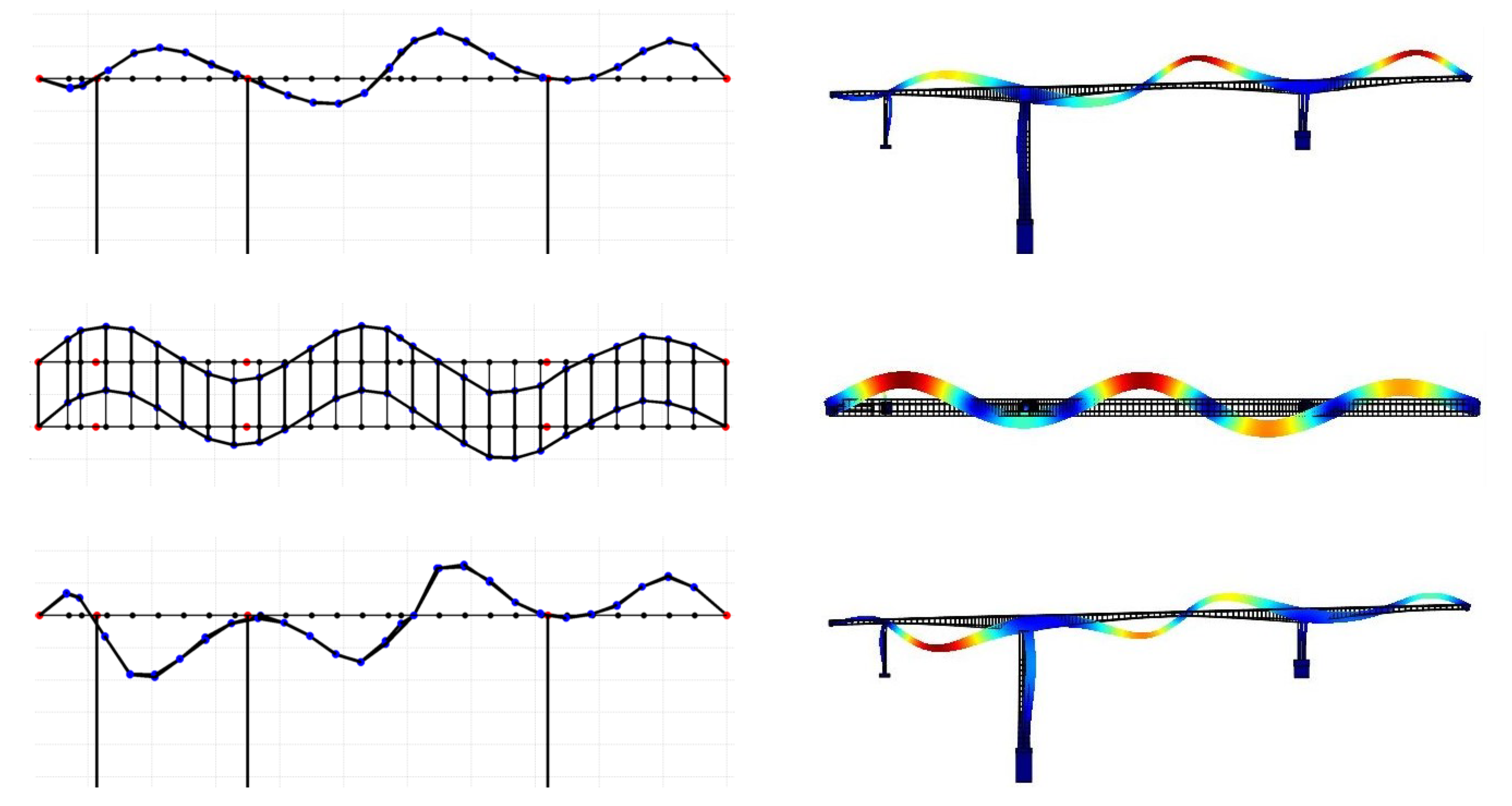
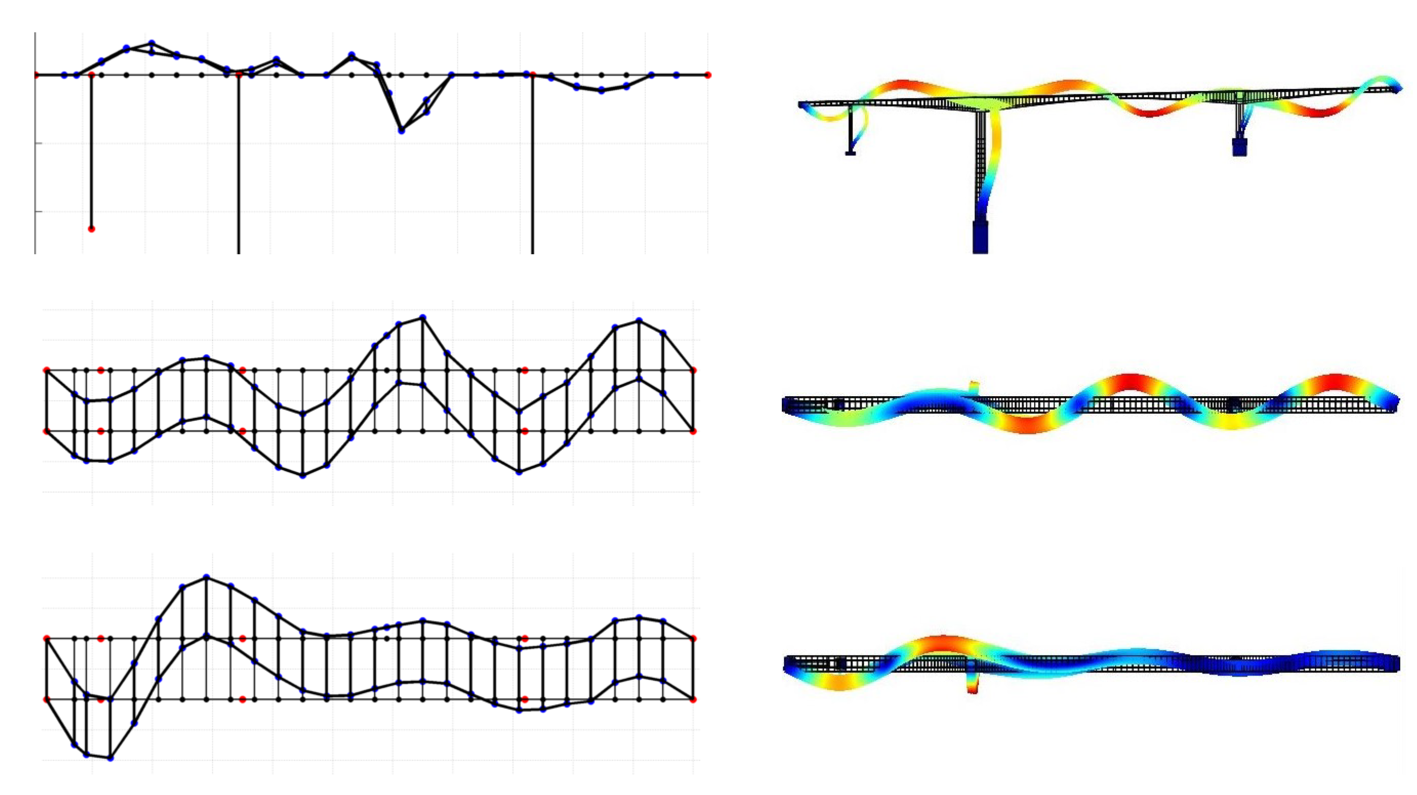
3. Application to Metsovo Bridge

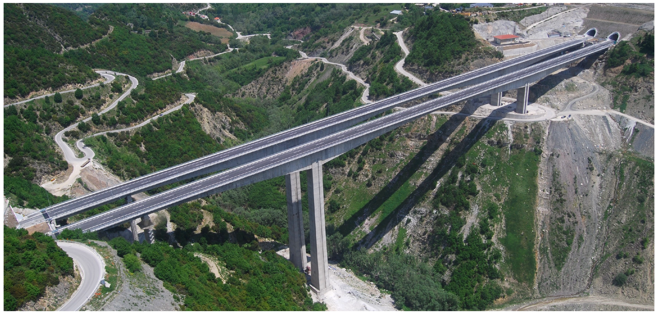
3.1. Description of Bridge

The ravine bridge of Metsovo (Anthohori–Anilio tunnel) of Egnatia Motorway is crossing the deep ravine of Metsovitikos river, 150 m over the riverbed. A picture of the bridge is shown in Figure 1. This is the highest bridge of the Egnatia Motorway, with the height of the tallest pier equal to 110 m. The total length of the bridge is 537 m. The bridge has 4 spans of length 44.78 m, 117.87 m, 235 m, 140 m and 3 piers of which the closest to the left side of the bridge (Figure 1), with height of 45 m, supports the boxbeam superstructure through pot bearings (movable in both horizontal directions), while the other two piers, with heights 110 m and 35 m, connect monolithically to the structure.

3.2. Finite Element Model of Bridge

The detailed geometry of the bridge is complicated because the deck and the piers have variable cross-sections and the deck is also inclined. A high fidelity FE model of the bridge is created using three-dimensional tetrahedral quadratic Lagrange finite elements. The model takes into account the potential soil-structure interaction by modeling the soil with large blocks of material and embedding the piers and abutments into these blocks. The nominal values of the moduli of elasticity of the deck and piers are selected to be the values used in design: 37 GPa for the deck and 34 GPa for the piers. The nominal value of the soil is taken to be 1 GPa. The largest size of the elements in the mesh is of the order of the thickness of the hollow deck cross-section. The size of the FE mesh is chosen to predict the first 20 modal frequencies and mode shapes of the bridge with sufficient accuracy. Several mesh sizes were tried, and an accuracy analysis was performed in order to find a reasonable trade-off between the number of degrees of freedom (DOF) of the model and the accuracy in the predicted modal frequencies. A mesh of 830,115 DOFs was kept for the bridge-soil model. This mesh was found to cause errors of the order of 0.1–0.5% in the first 20 modal frequencies, compared to the smallest possible mesh sizes which had approximately 3 million DOFs.

The intent is to build a high fidelity model that could, in future studies, be extended locally to incorporate nonlinear mechanisms activated during strong motion or deterioration phenomena. In this study the focus is to update a baseline linear model using low-intensity vibration measurements. In future studies, the availability of higher-intensity vibration measurements will provide data for improving modeling and updating parameters of nonlinear models introduced to represent localized nonlinear phenomena activated due to large vibrations or deterioration due to various damage mechanisms. Simplified beam models, although adequate for design purposes, are inadequate to use for setting up digital twins of structures so that are reliable under various operating conditions. Simplified modeling, for example with beam elements, does not offer an adequate representation of the system dynamics over the dynamic range activated by various operational conditions. Such simplified models are often inadequate for monitoring purposes and involve large model errors even for operational conditions under which the structure may be assumed to behave linearly.

3.3. Model Reduction Using CMS

The time required for a complete run of the FE model is approximately 2 min on a 8-core 3.20 GHz computer. Due to the thousands of forward model runs for different values of the model parameters that are required by the Bayesian computational tools, it is necessary to reduce the time required for a single model run. Model reduction is used to reduce the model size and thus the computational effort to manageable levels. Specifically, the parameterization-consistent CMS technique [34,35] based on the Graig-Bampton method [46] is applied to the bridge-soil FE model.

For this, the bridge is divided into 16 physical components with 15 interfaces between the components. Specifically, the deck is divided into six components or substructures of length 120 m, 120 m, 60 m, 50 m, 117 m and 70 m each. One component is assigned to each one of the three piers. Two components are introduced for the left and right abutments of the bridge. Five more components are introduced for the large solid blocks representing the flexibility of the soil at the connections with the three piers and the two abutments. This partition into component is one of the many alternative ones, introduced herein to demonstrate the capabilities of CMS technique for model reduction. Usually the partition of the structure into components is guided by the purpose of the analysis or the structural health monitoring goals. For example, components may be introduced to monitor and select models of nonlinearities activated by various operational conditions in isolated (localized) parts of a structure. The partition of a structure into components facilitates monitoring of the structural health, allowing the identification of the location and severity of sparse damage within a small subset of substructures.

For each component, it is selected to retain all modes that have frequency less than ${\omega }_{\max }=\rho {\omega }_c$, where ${\omega }_c=3.52$ Hz is the cut-off frequency selected to be equal to the 20th modal frequency of the nominal FE model. The $\rho$ values affect the computational efficiency and accuracy of the CMS technique. For $\rho =5$ selected for most components, a total of 170 internal DOFs out of the 814,080 are retained for all 16 components. The total number of DOFs of the reduced model is 16,205 which also includes 16,035 interface DOFs. It is clear that more than an order of magnitude reduction in the number of DOFs is achieved using CMS. The largest fractional error between the modal frequencies computed using the complete FE model and the ones computed using the CMS technique for $\rho =5$ falls below $0.2\%$. Thus a very good accuracy is achieved.

The large number of the interface DOFs can be reduced by retaining only a fraction of the constrained interface modes [34,49]. For each interface, only the modes that have frequency less than ${\omega }_{\max }=\nu {\omega }_c$ are retained, where $\nu$ is user and problem dependent. For $\nu =200$ selected for most interfaces, the largest fractional error for the lowest 20 modes of the structure falls below $0.43\%$. In particular, for $\nu =200$ and $\rho =5$ the reduced system has 1891 DOFs from which 170 generalized coordinates are fixed-interface modes for all components and the rest 1721 generalized coordinates are constrained interface modes [34]. A trade-off was made between reducing the model as much as possible (fewer kept DOFs) and keeping the accuracy of the predicted modal frequencies as close as possible to those of the unreduced model. It should be noted that further reductions are possible using an enhanced substructuring technique where the dynamics contribution of several kept modes is replaced by their static contribution [47].

Thus, using CMS a drastic reduction in the number of DOFs is obtained which can exceed two orders of magnitude, without sacrificing the accuracy with which the lowest 20 modal frequencies are computed. The time to solution for one run of the reduced model is of the order of a few seconds which should be compared to approximately 2 min required for solving the unreduced FE model.

Moreover, for nonlinear models of structures, especially models where local nonlinearities are mainly activated, the model reduction techniques can also be applied to reduce the models of components of the structure that behave linearly under various operational conditions [35,48].

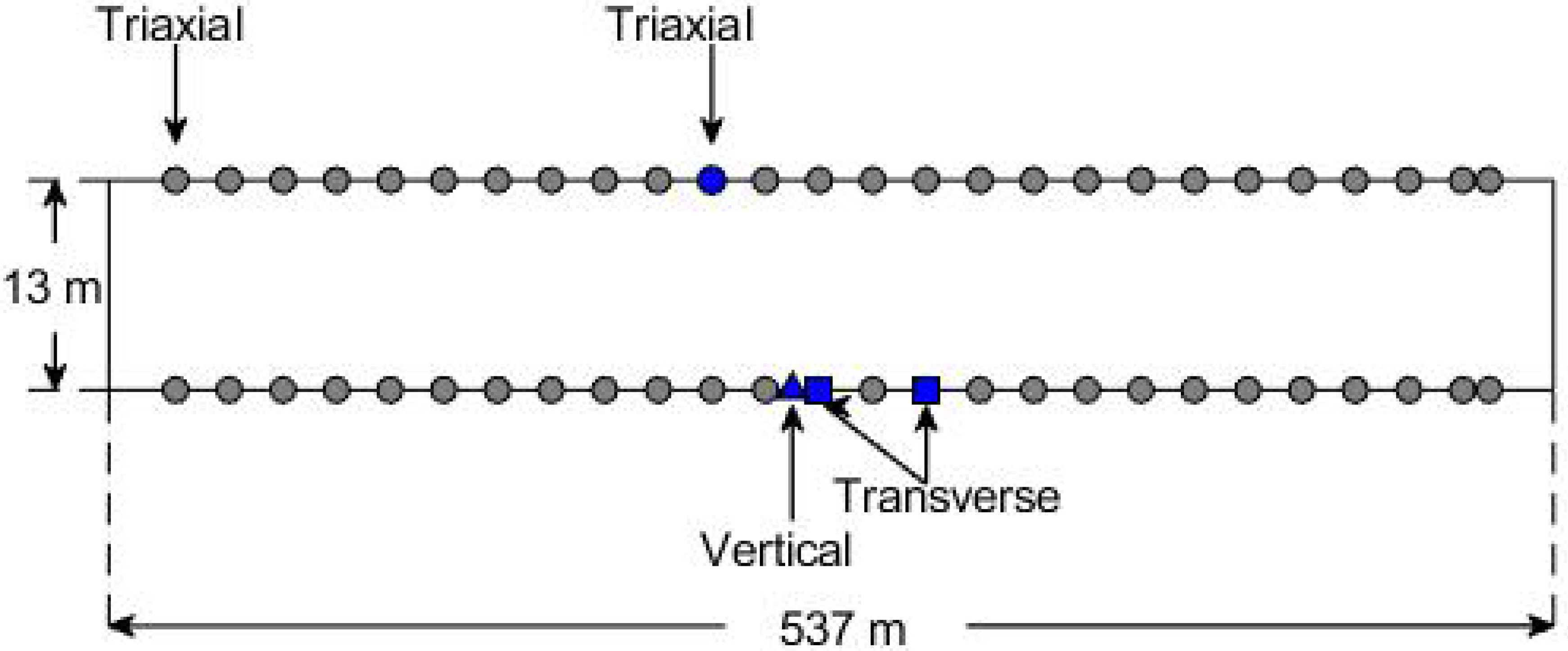
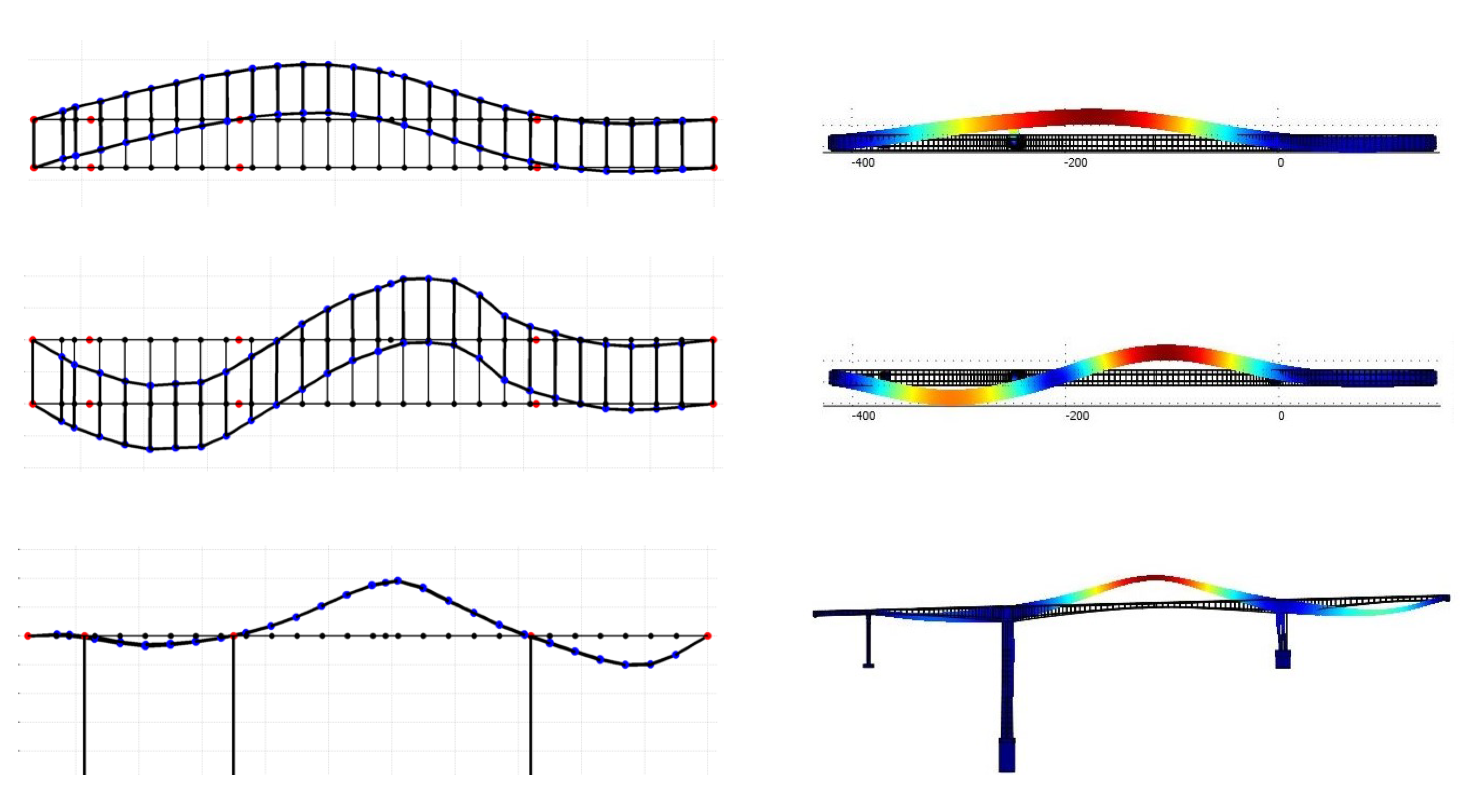
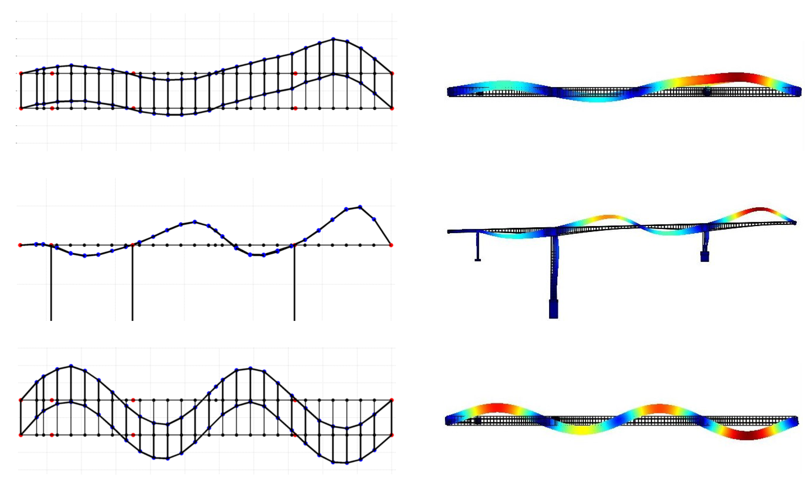
3.4. Experimental Modal Identification

The testing system consist of a movable array of servo-accelerometers that are usually being installed on the bridge deck (sidewalks or pavement surface) or inside the box beam internal voids to measure the vibrations (accelerations) of the bridge under ambient excitations. The available measurement system consisted of five triaxial and three uniaxial accelerometers paired with a 24-bit data recording system, a GPS module for synchronization between sensors, and a battery pack. The system is wireless and can be easily moved from one location in the structure to another. The recorder can connect with a laptop through wired (Ethernet) or wireless (Wi-Fi) connection to be set up in the desired way (sampling rate, recording duration, repeater recordings etc) or view the measurements while they are being recorded for quality checking. Given the limited number of sensors and the large length of the deck, the entire length of the deck was covered in 13 sensor configurations, shown in Figure 2. For each configuration the recording lasted 20 min at a sampling rate of 100 Hz. Each triaxial sensor was positioned on the bridge sidewalks such that it measures along the transverse, vertical and longitudinal directions of the bridge deck. One triaxial and three uniaxial sensors (one vertical and two horizontal transverse) remained in the same position throughout the measurements, in order to provide common measurement points amongst different configurations such as to enable the assembling of the total mode shape from partial mode shape components measured from the different configurations [30,32]. The use of more than one reference sensors per direction guarantees the redundancy of the measuring scheme in case one sensor is placed at the node of the modeshape. The wireless feature of the measurement system allows the execution of all recordings over the 13 sensor configurations in a single day. The recorded responses are mainly due to road traffic, which ranged from light vehicles to heavy trucks, and environmental excitation such as wind loading, which classifies this case as ambient (operational) modal identification.

The Bayesian operational modal analysis methodology [9,10] is used to estimate the modal frequencies, mode shapes and damping ratios for each sensor configuration. The mode shapes are assembled from the local mode shapes of each configuration using the methodology proposed by Au [32]. The full mode shapes are produced at all 159 sensor locations covered by the 13 sensor configurations. The components along the longitudinal direction of the bridge deck are ignored. Only the components along the transverse and vertical direction of the bridge deck are processed. The output-only vibration measurement for some of the 13 sensor configurations were not reliable enough to estimate the mode shape components at higher modes. As a result, it was not possible to assemble the mode shapes for more than 12 modes. Thus these mode shapes were excluded from the analysis. Specifically, the first 20 modal frequencies and modal damping ratios of the bridge were identified, along with 11 mode shapes. The mode shapes of all the modes up to the 12th were identified, except the 10th mode which was very poorly identified and also excluded from the date set.

Table 1. First 20 experimentally identified modal frequencies of the the Metsovo bridge compared with the modal frequencies predicted by the nominal FE model of the bridge. MAC values between identified and model predicted mode shapes are also shown.

Mode	Experimental	Nominal Model	Mode Shape
	Frequency (Hz)	Frequency (Hz)	MAC Value
1	0.306	0.293	0.991
2	0.603	0.574	0.955
3	0.623	0.619	0.978
4	0.965	0.849	0.935
5	1.047	1.050	0.969
6	1.139	1.070	0.965
7	1.428	1.388	0.972
8	1.697	1.578	0.966
9	2.005	1.690	0.878
10	2.303	1.966	0.85
11	2.367	2.156	0.972
12	2.590	2.317	0.971
13	2.723	2.500
14	3.086	2.745
15	3.127	2.815
16	3.480	2.876
17	3.861	2.950
18	4.058	3.320
19	4.210	3.381
20	4.410	3.521

presents the mean and standard deviation of the experimentally identified modal frequencies for all 20 identified modes of the Metsovo bridge. It also compares the identified frequencies and mode shapes with those predicted by the nominal FE model. In particular, the experimental and nominal model predicted mode shapes are compared using their MAC value which is a scalar measure of correlation between two mode shapes ranging from 0 to 1, with a value of 1 indicating perfect correlation. The identified mode shapes are shown in Figure A1, Figure A2, Figure A3 and Figure A4 of Appendix A and compared with the corresponding mode shapes predicted by the nominal FE model of the bridge. From both the MAC values of Table 1 and mode shapes of Figure A1, Figure A2, Figure A3 and Figure A4 it can be clearly seen that the mode shapes predicted by the nominal FE model match very accurately the corresponding experimentally identified mode shapes with MAC values higher than 0.95 for the 11 identified mode shapes (except mode 9 which has a MAC value of 0.87). However, there appears to be a significant mismatch between the experimental and nominal FE model modal frequencies which indicates that a finite element model updating should be performed in order to achieve a closer fit between the model predicted and the experimentally identified modal frequencies.

4. Model Updating Results

The FE model of the bridge–soil system is parameterized using three parameters associated with the modulus of elasticity of the deck (${\theta }_1$), piers (${\theta }_2$) and soil (${\theta }_3$). The model parameters multiply the nominal values of the corresponding moduli of elasticity for the deck (37 GPa ), the piers (34 GPa) and the soil (1 GPa). The nominal values for the deck and piers are reasonable estimates since they are the moduli of elasticity of the concrete used in design and therefore their updated values of ${\theta }_1$ and ${\theta }_2$ are expected to lie close to 1. However, as far as the soil is concerned, its nominal value is only a rough estimate, based on soil property measurements conducted at the site of the bridge. Therefore, its nominal value should be dealt with a large uncertainty in the model updating procedure. These modeling considerations regarding the initial parameter uncertainties are taken into account in the Bayesian framework through the prior PDF. It should be noted that a simplified uniform parameterization involving a small number of parameters is considered in order to avoid possible unidentifiability issues and enable the comparison between the two different likelihood formulations.

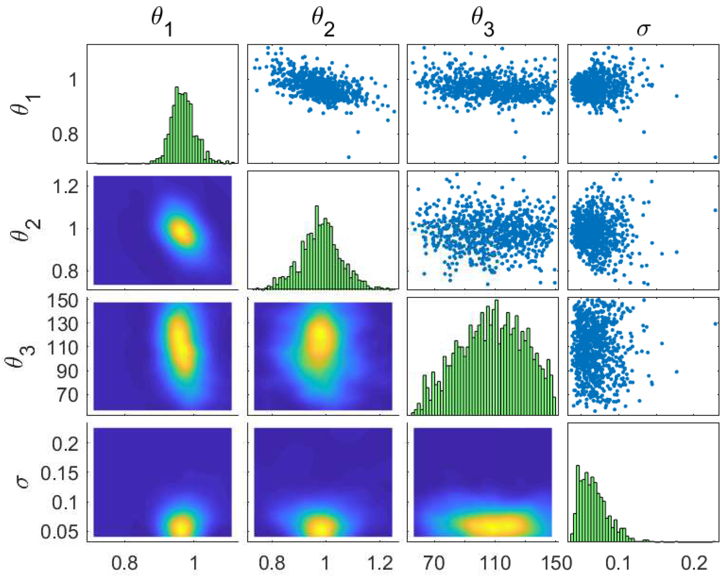
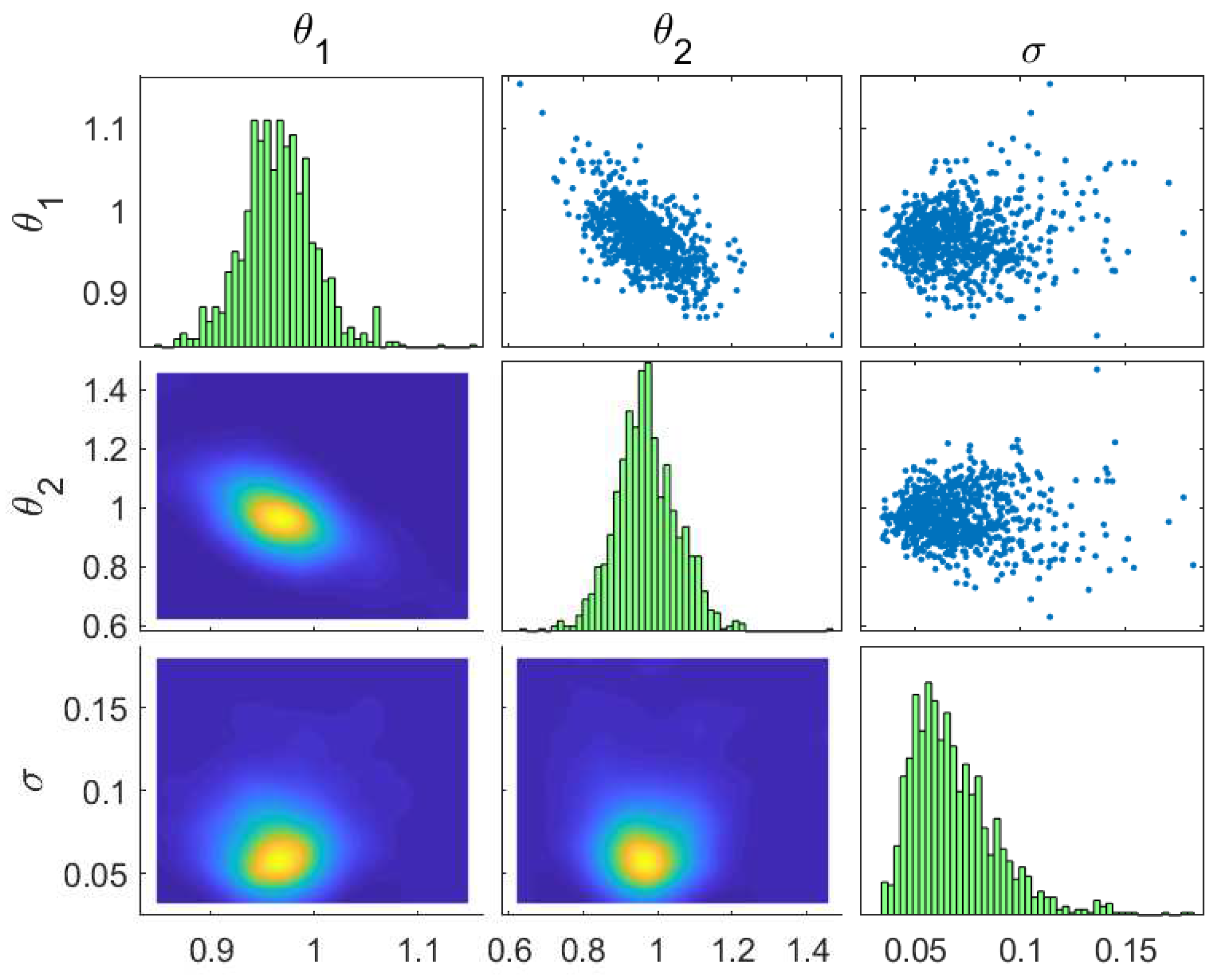
4.1. Model Updating Using Modal Frequencies Only

First, the FE model of the bridge-soil system is updated using only a subset of the experimentally identified modal frequencies. This approach allows one to use the rest of the frequencies in order to validate the updated model by checking its predictive capabilities with data that was not used in the updating. Specifically, the first 15 identified modal frequencies are used to estimate the model parameters and their uncertainty, while the other five modal frequencies are used in order to validate the updated model. For 11 out of the 20 modes we use mode correspondence through the MAC values to associate the experimentally identified and model predicted modal properties. It was found that the i-th experimentally identified mode corresponds to the i-th mode predicted by the model. For modes higher than 12 for which there no mode shape identified from experimental data, we match the modal frequencies based only on the number of mode identified or predicted by the FE model, with modal frequencies arranged in an ascending order.

4.1.1. Flexible-Soil Model

The prior distribution for the parameters are assumed to be uniform with bounds in the domain $[0.5,1.5]\times [0.5,1.5]\times [0.1,1000]$ for the deck, pier and soil parameters respectively, and in the domain $[0.001,1]$ for the prediction error parameter ${\sigma }_{\omega }$. The domain for the soil parameter was deliberately chosen much larger in order to account for the large uncertainty in the values of the soil stiffness and be able to explore the full effect of the soil stiffness on the model behavior.

Model updating results are obtained using the parallelized TMCMC algorithm [33,36] for the bridge–soil FE model. The TMCMC is used to generate samples from the posterior PDF of the structural model and prediction error parameters. These samples represent the posterior PDF and therefore our updated state of knowledge about the parameters given the experimental data. After the posterior samples are drawn the parameter uncertainty is propagated to the predictions of the first 20 modal frequencies of the bridge. This is done in order to check the fit of the updated model with the experimental frequencies that were used to perform the model updating, but also with the next five modal frequencies that were not included in the data set. In all TMCMC runs, the following selection is made: $TolCov=1.0$, $\beta =0.2$ [33]. The number of samples used per TMCMC stage are 1000, resulting in a total runtime of approximately 10 minutes using the reduced 1.891 DOF model in a 8-core 3.20 GHz computer.

The TMCMC samples which represent the posterior PDF are visualized through their marginal distributions and two-dimensional (2D) projections in Figure 3. The sample statistics are shown in

Table 2. Quantiles of posterior samples for all parameters. The x% quantile for a parameter is defined as the level that corresponds to x% of the values of the parameter over all TMCMC samples, arranged in increasing order, to fall below this level.

	${\theta }_1$	${\theta }_2$	${\theta }_3$	$\sigma$
$5\%$ Quantile	0.919	0.844	70.428	0.044
$50\%$ Quantile	0.968	0.981	110.23	0.065
$95\%$ Quantile	1.029	1.115	150.20	0.105

. The posterior parameter uncertainty is propagated through the model using the samples to yield the robust model predictions of the lowest 20 modal frequencies. The fit is shown in Figure 4. The predicted modal frequencies are normalized with respect to the experimentally-identified frequencies for comparison convenience. Therefore, values close to 1 are close to the experimental frequencies. The improvement achieved by the updated model compared to the nominal model is evident. For most modes the experimental frequency lies within the predicted 5–95% interval or very close to it, and in all cases the error is of the order of 3–4% which should be compared to the error of the nominal model which is of the order of 10% to 20% for some modes. This is a strong indication of the need for model updating in order to improve the accuracy and predictive capability of the updated model.

Regarding the parameters, it can be seen that the updated values of the deck and pier parameters lie close to 1 as expected, and slightly below it. The mean values for the deck and pier stiffness parameters are estimated to be approximately 0.95 and 0.98 times their nominal values with uncertainties of the order of $5\%$ and $12\%$ respectively. From the $({\theta }_1-{\theta }_2)$ 2D projection of Figure 3 it is evident that a negative correlation exists between the deck and pier stiffnesses. This is reasonable since an increase in the stiffness of the deck can be counterbalanced by a decrease in the stiffness of the piers such that the modal frequency values are maintained, and vice versa.

As far as the updated soil stiffness is concerned, the only (but important) new information that is acquired by the model updating is that its value can be arbitrarily large, as long as it exceeds a threshold. The threshold value appears to be approximately 70 which is the minimum value that the updated soil parameter can attain, as seen from its posterior marginal distribution in Figure 3. A value of 70 implies a soil modulus of elasticity of 70 GPa which is more than double of the updated (and nominal) value of the pier modulus of elasticity (34 GPa). The soil parameter can increase substantially above this value without affecting the fit with the experimental data, that is, without causing any variation in the predicted modal frequencies of the model. Considering that the uniform prior bound for the soil stiffness was set to $[0.1,1000]$ it is obvious that lower values which would attribute to the soil some flexibility similar to that of the piers are not preferred. In addition, the large posterior uncertainty in soil property indicates that the modal frequencies are insensitive to the values of the soil modulus of elasticity for these high values of the soil property. This insensitivity is due to the low vibration levels recording from ambient operational conditions of the bridge.

4.1.2. Two-Parameter Stiff-Soil Model

The results obtained from the flexible-soil model suggest that the bridge appears to be fixed to the ground and the modal properties predicted by the model are insensitive to the soil modulus of elasticity. This leads to introducing a second model, which corresponds to eliminating the soil parameter by fixing its value to a large value as suggested by its posterior marginal distribution of Figure 3, simulating the very stiff soil conditions which were found from the first model. Therefore, the new two-parameter model has as parameters the modulus of elasticity of the deck (${\theta }_1$) and piers (${\theta }_2$), while the soil parameter is fixed to 100.

The posterior samples for the two-parameter model are visualized using their marginal distributions and 2D projections in Figure 5. The sample statistics are shown in

Table 3. Quantiles of posterior samples for all parameters.

	${\theta }_1$	${\theta }_2$	$\sigma$
$5\%$ Quantile	0.908	0.835	0.044
$50\%$ Quantile	0.965	0.966	0.065
$95\%$ Quantile	1.022	1.108	0.108

. The posterior parameter uncertainty is propagated through the model using the samples to yield the robust model predictions of the lowest 20 modal frequencies. The fit is shown in Figure 6. Note that in Figure 6 the predictions of the nominal model are closer to the experimental due to the increase of the soil parameter to the fixed value of 100 in order to simulate the stiff-soil conditions, which led to an increase of the modal frequencies of the nominal model. It can be seen that, as expected, the model updating results both in terms of the updated values of the parameters and in terms of the fit with the data are almost identical to the results obtained from the three-parameter model in Figure 4.

This is also confirmed using the Bayesian model selection framework [38] to compute the evidence $p\left(D\right|M_i)$ for the two models, taking into account both the complexity of the models in the form of the number of its parameters and the fit they achieve with the data in order to obtain a trade-off between the two. The TMCMC algorithm provides the values of the evidence of each model as a by-product of the algorithm. Therefore, by performing model updating on both models they can be easily compared using their evidence values. The log-evidence for the three-parameter flexible-soil model was found to be 2.52, which is slightly less than the evidence value 2.55 of the two-parameter stiff-soil model. Bayesian model selection slightly rewards the stiff-soil model for having one less parameter than the flexible-soil model.

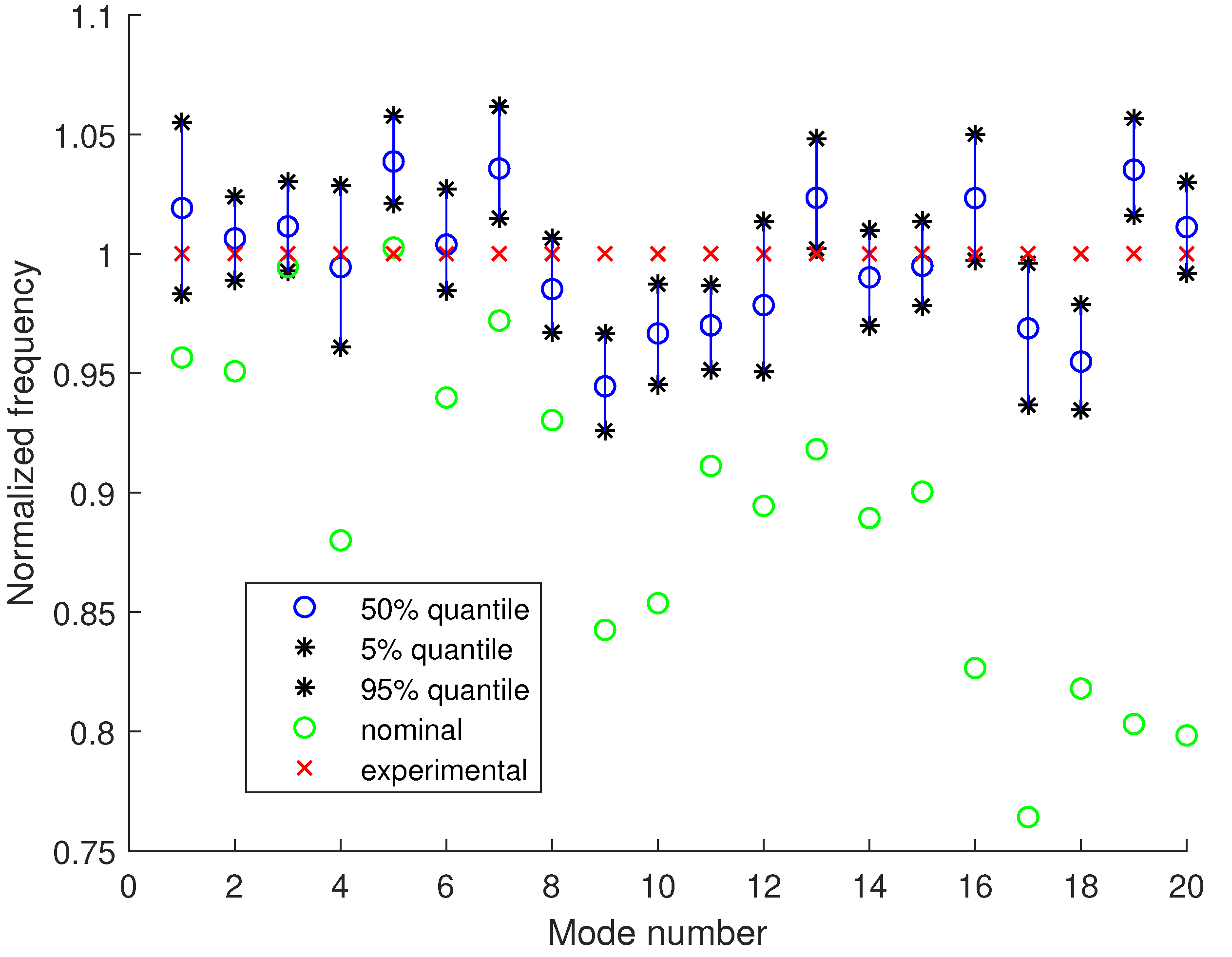
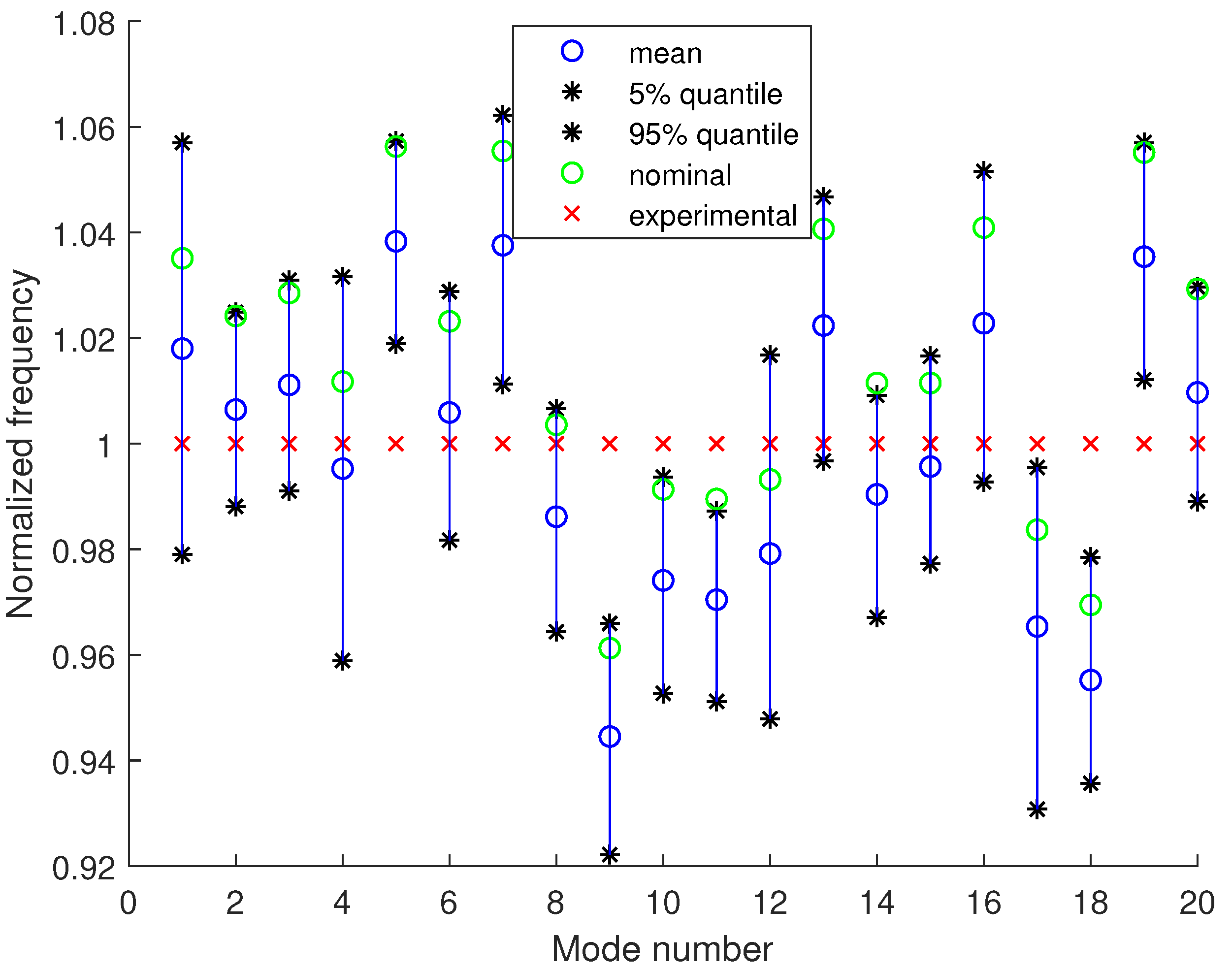
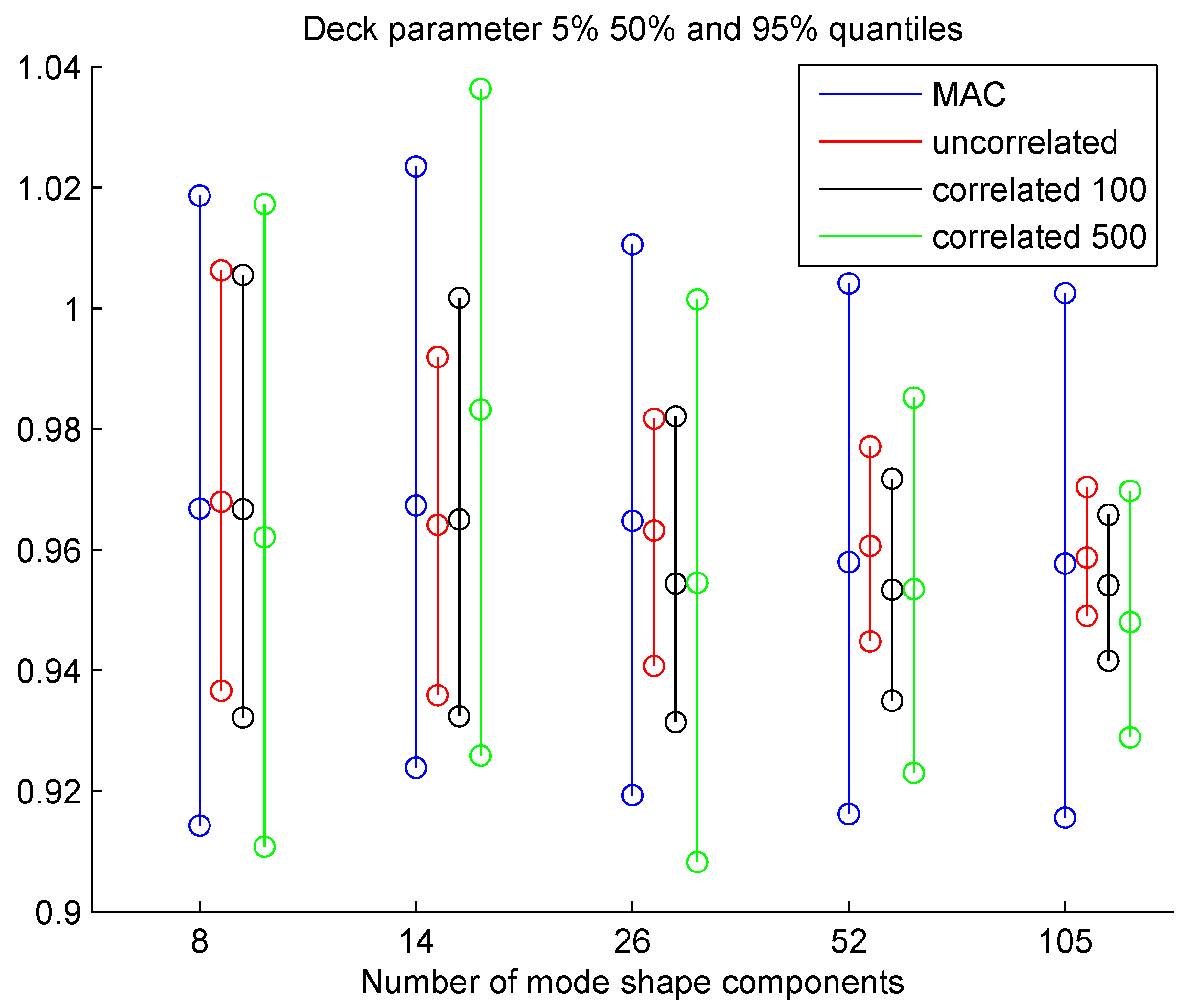
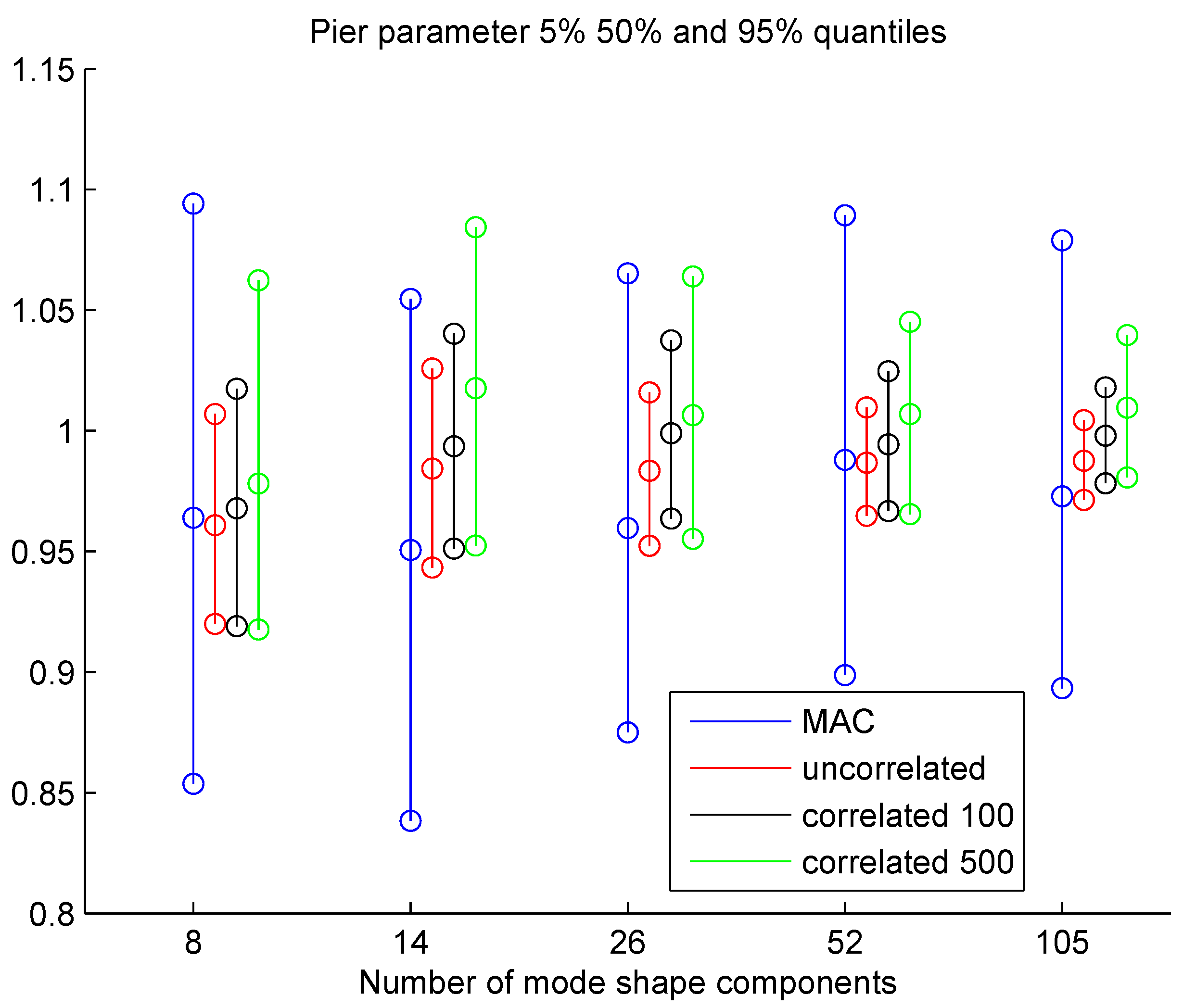
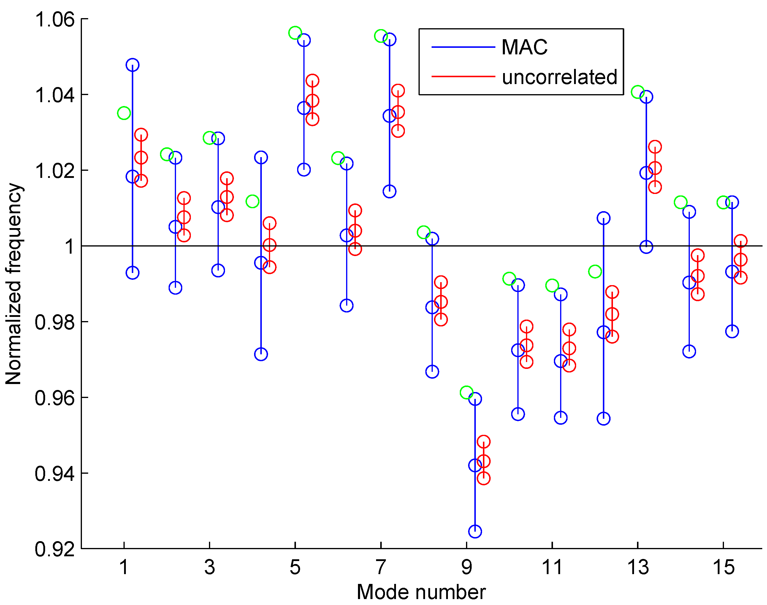
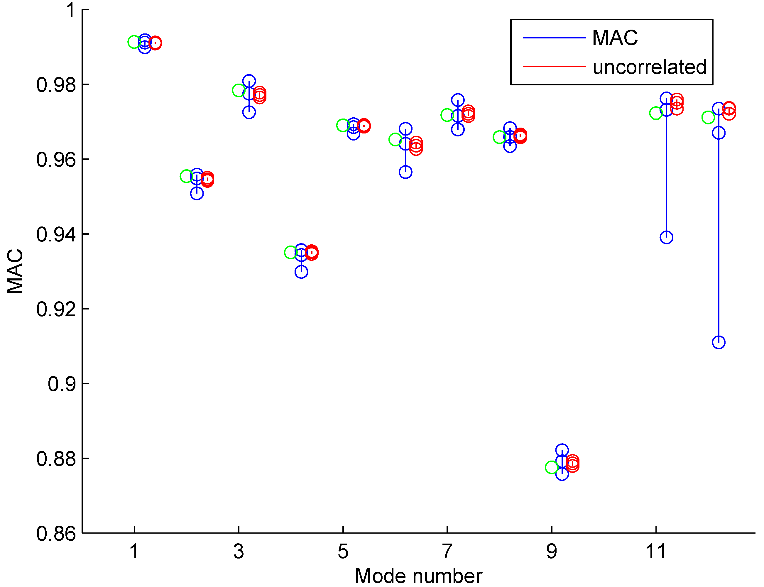
4.2. Model Updating Using Modal Frequencies and Mode Shapes

Next we also include the mode shapes into the dataset used for model updating. Both the vector-based (Section 2.1.1) and the MAC-based (Section 2.1.2) formulations of the likelihood are used to update the deck and pier model parameters of the two-parameter FE model. Regarding the vector-based likelihood formulation, two cases of mode shape component correlation are examined, namely the uncorrelated and exponentially correlated cases. For the exponentially correlated case, two correlation lengths are examined: ${\lambda }_r=100$ m and ${\lambda }_r=500$ m for all r values.

A crucial aspect of the analysis is to examine the effect of the number of mode shape components (sensors) used in the likelihood function on the model parameter uncertainty and uncertainty in model predictions. In order to study this effect, five different sensor configurations are considered with 8, 14, 26, 52, 105 measured DOF. For each configuration the sensors are selected to be uniformly spread along the bridge deck. In addition, the configuration with a larger number of measured DOF includes the measured DOF contained in configurations with smaller number of DOF. In this way, the information contained in the data of a configuration with a given number of measured DOF, includes the information contained in the data of a configuration with smaller number of DOF. In each sensor configuration case, half of the DOF are transverse (sensors measuring in the transverse direction) and half are vertical. The longitudinal DOF were not included due to their negligible contribution in the identified mode shapes compared to the transverse and vertical components. The transverse and vertical DOF were selected to be in the same point, that is, eight DOF correspond to four different pairs of transverse and vertical DOF in the same point. The case of 52 DOF corresponds to the complete set of measured DOF in the one side of the bridge, while the case of 105 DOFs corresponds to measured DOFs on both sides of the bridge. Due to the type of the vertical and transverse mode shapes, the mode shape components at one side of the bridge provide exactly the same information as the mode shape components at the opposite side of the bridge. So the case of 105 measured DOFs should not be expected to provide additional information as compared to the case of 52 sensors.

Figure 7 and Figure 8 show the posterior parameter uncertainty for the deck and pier parameters of the model as a function of the number of sensors, for each case of likelihood formulation. The posterior uncertainty for each parameter is shown in terms of the $5\%$, $50\%$ and $95\%$ quantiles of the marginal posterior samples obtained from the TMCMC algorithm for the corresponding parameter.

It should be noted that the vector-based likelihood formulations for the mode shapes (uncorrelated and the two exponentially correlated models with spatial correlation lengths of 100 and 500) result in a steady reduction in the posterior uncertainty of both model parameters (deck and pier parameters), as the number of mode shape components used in the likelihood is increased. This is in agreement with the Bayesian theory of parameter estimation, which suggests that as the number of data points used in the likelihood is increased the posterior uncertainty is reduced. Indeed, in the vector-based formulations, the mode shapes are treated as vectors of size equal to the number of their used components. Therefore, the total number of data points used in the likelihood is increased as we use more of the identified mode shape components.

However, as more mode shape components are used, the locations of the sensors become increasingly closer to each other. The shorter characteristic length corresponding to the lowest 10 identified mode shapes is approximately 130 m as one can observe from Figure A1, Figure A2, Figure A3 and Figure A4 of Appendix A. As the number of sensors increase to 25 or higher, the shortest distance between sensors becomes a fraction of the characteristic length of the identified mode shapes and so there is redundant information contained in the measured mode shape data. In fact no new information is expected from sensors placed at a distance that is sufficiently smaller than the characteristic length of a mode shape. Especially in the case of 52 and 105 DOFs (which correspond to the entire set of identified mode shape components in one side and both sides of the bridge) we do not expect the inclusion sensor information from the second side to further reduce the posterior uncertainty. This is because the identified mode shape components at the two sides of the bridge are almost identical, and therefore including the second side does not provide any new information about the transverse and vertical mode shapes. The same holds true to a lesser degree for the other cases of DOFs because the sensors are getting closer as we use more of them and contain very similar information. So we would expect the posterior uncertainty to initially reduce as we increase the number of sensors, but only up to a certain point, and then remain practically constant as we include more sensors due to the redundant information provided from the closely spaced sensors or sensors placed at opposite sides of the bridge.

This expected behavior is opposite to what is observed using the vector-based formulations of the likelihood for the mode shapes. Even adding the sensors at the second side of the bridge (which provide identical information with the sensors in one side) seems to further reduce the posterior parameter uncertainty for both the deck and pier parameters. Correlated prediction error models have been suggested to alleviate this situation, and have been successful in some cases, but these correlated prediction error models are very difficult to postulate correctly in practice and could otherwise lead to erroneous results [41].

A totally different behavior is observed under the MAC-based likelihood formulation for the mode shapes. The posterior uncertainty does decrease at first, but then it stabilizes and is practically unaffected by the inclusion of more sensors after some point. Specifically, we see that when the number of sensors increase from 8 to 14 and 26, there is a reduction in the uncertainty, but after that point the uncertainty gets stabilized and is not affected by doubling the number of sensors to 52 and eventually to 105. This happens because in the MAC-based formulation the mode shapes are not utilized as vectors, but as scalar MAC values, reducing the effective number of independent data points for each mode shape to one, instead of as many as the number of mode shape components. It is also important to note that the overall parameter uncertainty is much larger compared to the vector-based formulations indicating that no significant information gain occurs by further increasing the number of sensors.

A quantitative assessment is given in

Table 4. Deck and pier posterior uncertainty ($90\%$ credible interval) versus the number of sensors for the vector-based (uncorrelated) and MAC-based formulations of likelihood.

NDOF	Uncorrelated		MAC
	Deck	Pier	Deck	Pier
8	0.070	0.087	0.104	0.241
14	0.056	0.083	0.100	0.216
26	0.041	0.064	0.091	0.190
52	0.032	0.045	0.088	0.191
105	0.021	0.033	0.087	0.186

which shows the 5–95% credible interval for the posterior PDF of the deck and pier model parameters for different number of sensors under the vector-based (uncorrelated) and MAC-based likelihood formulations. It can be seen that the vector-based (uncorrelated) formulation keeps reducing the posterior uncertainty of the model parameters as the number of sensors increase, whereas the uncertainty is maintained for the MAC-based likelihood formulation for 26, 52 and 105 sensors.

Uncertainty Propagation to Modal Frequencies and MAC Values

The uncertainty in the model parameter values is propagated to modal frequencies in Figure 9 and MAC values in Figure 10. Results are presented for the vector-based (uncorrelated) and MAC-based formulations using 105 DOFs for the mode shapes (sensors on both sides of the bridge). The modal frequency predictions in Figure 9 are normalized with respect to the experimental modal frequencies.

The larger posterior parameter uncertainties obtained with the MAC-based likelihood formulation result in larger uncertainties in the predicted modal frequencies compared to the uncertainties predicted by the vector-based (uncorrelated) likelihood formulation. The experimental frequencies are included within the 5–95% credible intervals predicted by the MAC-based likelihood formulation for 10 out of the 15 modes (the black horizontal line crosses the 5–95% interval except for 5 modes), while the modal frequency predictions obtained from the uncorrelated model do not include the experimental frequencies within the 5–95% credible intervals, except from only three modes (4-th, 6-th and 15-th modes). Therefore, the predictions obtained from the vector-based likelihood formulation have more error associated with them compared with those obtained from the MAC formulation, when checking against the experimentally identified modal frequencies. Thus, the MAC-based likelihood formulation has better predictive capabilities than the vector-based likelihood formulation, in the sense that the predicted uncertainty bounds either fully contain or are closer to the experimental modal frequencies.

The predicted MAC values presented in Figure 10 have also larger uncertainties as expected under the MAC formulation, but the difference is not as obvious as in the modal frequencies (except for mode shapes 11 and 12 which have large uncertainties in their MAC value). The MAC values are well above 0.95 (with the exception of mode shape 9 which has a MAC value of 0.88), indicating a very close match between the experimental and model predicted mode shapes. Note that the MAC values obtained from the nominal model (green circles in Figure 10) are contained within the credible intervals of the vector-based likelihood formulation. This indicates that the mode shapes are highly insensitive to changes in the values of the two model parameters. However, it was demonstrated that inclusion of the mode shapes in the likelihood function does play an important role in the resulting posterior uncertainty of the model parameters, thereby affecting the uncertainty in the predicted modal frequencies.

Based on the uncertainty results for the model parameters presented in Figure 7 and Figure 8, it is expected that the uncertainty in the modal frequencies and mode shapes presented in Figure 9 and Figure 10 will be unaffected for the MAC-based likelihood formulation when the number of sensors is reduced from 102 to 54 or 27. However, for the vector-based likelihood formulation the uncertainty in the modal frequencies and MAC values is expected to increase due to the increase in the parameter uncertainties in Figure 7 and Figure 8 when the number of sensors is reduced from 102 to 54 or 27.

5. Conclusions

A Bayesian framework was presented for FE model updating of structures using experimentally identified modal frequencies and mode shapes. A novel way for including the mode shapes into the likelihood formulation was proposed by assigning a probability model to the MAC values between the experimentally identified and model predicted mode shapes, summarizing the information in the mode shapes in scalar features instead of vectors as it is conventionally done in existing formulations. The MAC-based likelihood formulation provides uncertainty bounds of the model parameters which are consistent with expectations as the number of sensors increases, while the vector-based likelihood formulation fail to properly account for the redundant information contained in the mode shape components, especially for relatively closely spaced sensors. The merits of the new likelihood formulation in relation to existing formulations were explored by updating the FE model of the Metsovo bridge. A high fidelity FE element model of hundreds of thousand of DOF was developed to accurately model the dynamic behavior of the bridge. TMCMC was used to perform the model updating, while model reduction techniques were effectively employed to drastically reduce the computational effort to manageable levels.

It was demonstrated that the model-updating results obtained from the MAC-based likelihood formulation differ significantly from the ones obtained by classical vector-based likelihood formulations. Specifically, the posterior parameter uncertainty was found to be stabilized as the number of sensors in the mode shapes are increased or the distance between sensors is relatively less than the characteristic lengths of the identified mode shapes, or as extra mode shape components (at the opposite side of the bridge), containing redundant information, are added. In contrast, the uncertainty in the model parameters for the classical vector-based likelihood formulation is decreasing as the number of sensors increases, which is counter-intuitive since it does not take into account the redundant information contained in measurements. This decrease in uncertainty is observed for spatially uncorrelated and exponentially correlated prediction error models considered in this study. Propagating the uncertainty in modal frequencies and MAC values, it is demonstrated that the MAC-based likelihood formulation provides wider uncertainty bounds that contain the experimental data. In contrast, the uncertainty bound predicted by the vector-based likelihood formulation fail to fit the experimental data since there is a significant distance of the experimental data from the predicted uncertainty bounds.

References

1. Friswell, M.I.; Mottershead, J.E. Finite Element Model Updating in Structural Dynamics; Springer Science + Business Media Dordrecht: Berlin, Germany, 1995. [Google Scholar] [CrossRef]
2. Sehgal, S.; Kumar, H. Structural Dynamic Model Updating Techniques: A State of the Art Review. Arch. Comput. Methods Eng. 2015. [Google Scholar] [CrossRef]
3. Vanik, M.W.; Beck, J.L. A Bayesian probabilistic approach to structural health monitoring. Struct. Health Monit. 1998, 3243, 140–151. [Google Scholar] [CrossRef] [Green Version]
4. Vanik, M.W.; Beck, J.L.; Au, S.K. Bayesian probabilistic approach to structural health monitoring. ASCE J. Eng. Mech. 2000, 126, 738–745. [Google Scholar] [CrossRef] [Green Version]
5. Yuen, K.V. Bayesian Methods for Structural Dynamics and Civil Engineering; John Wiley & Sons: Singapore, 2010. [Google Scholar] [CrossRef]
6. Yuen, K.V.; Beck, J.L.; Katafygiotis, L.S. Efficient model updating and health monitoring methodology using incomplete modal data without mode matching. Struct. Control Health Monit. 2006, 13, 91–107. [Google Scholar] [CrossRef]
7. Mustafa, S.; Matsumoto, Y. Bayesian model updating and its limitations for detecting local damage of an existing truss bridge. J. Bridge Eng. 2017, 22, 04017019. [Google Scholar] [CrossRef]
8. Yuen, K.V.; Beck, J.L.; Katafygiotis, L.S. Probabilistic approach for modal identification using non-stationary noisy response measurements only. Earthq. Eng. Struct. Dyn. 2002, 31, 1007–1023. [Google Scholar] [CrossRef]
9. Au, S.K. Fast Bayesian ambient modal identification in the frequency domain, Part I: Posterior most probable value. Mech. Syst. Signal Process. 2012, 26, 60–75. [Google Scholar] [CrossRef]
10. Au, S.K. Fast Bayesian ambient modal identification in the frequency domain, Part II: Posterior uncertainty. Mech. Syst. Signal Process. 2012, 26, 76–90. [Google Scholar] [CrossRef]
11. Au, S.K.; Zhang, F.L.; To, P. Field observations on modal properties of two tall buildings under strong wind. J. Wind Eng. Ind. Aerodyn. 2012, 101, 12–23. [Google Scholar] [CrossRef]
12. Au, S.K.; Zhang, F.L. Ambient modal identification of a primary–secondary structure by Fast Bayesian FFT method. Mech. Syst. Signal Process. 2012, 28, 280–296. [Google Scholar] [CrossRef]
13. Au, S.K.; Zhang, F.L.; Ni, Y.C. Bayesian operational modal analysis: Theory, computation, practice. Comput. Struct. 2013, 126, 3–14. [Google Scholar] [CrossRef]
14. Zhang, F.L.; Au, S.K. Fundamental two-stage formulation for Bayesian system identification, Part II: Application to ambient vibration data. Mech. Syst. Signal Process. 2016, 66, 43–61. [Google Scholar] [CrossRef]
15. Zhang, F.L.; Ni, Y.C.; Au, S.K.; Lam, H.F. Fast Bayesian approach for modal identification using free vibration data, Part I–Most probable value. Mech. Syst. Signal Process. 2016, 70, 209–220. [Google Scholar] [CrossRef]
16. Ni, Y.C.; Zhang, F.L.; Lam, H.F.; Au, S.K. Fast Bayesian approach for modal identification using free vibration data, Part II—Posterior uncertainty and application. Mech. Syst. Signal Process. 2016, 70, 221–244. [Google Scholar] [CrossRef]
17. Kuok, S.; Yuen, K. Investigation of modal identification and modal identifiability of a cable-stayed bridge with Bayesian framework. Smart Struct. Syst. 2016, 17, 445–470. [Google Scholar] [CrossRef]
18. Ni, Y.; Lu, X.; Lu, W. Operational modal analysis of a high-rise multi-function building with dampers by a Bayesian approach. Mech. Syst. Signal Process. 2017, 86, 286–307. [Google Scholar] [CrossRef]
19. Beck, J.L.; Au, S.K. Bayesian updating of structural models and reliability using Markov chain Monte Carlo simulation. J. Eng. Mech. ASCE 2002, 128, 380–391. [Google Scholar] [CrossRef]
20. Beck, J.L.; Katafygiotis, L.S. Updating models and their uncertainties. I: Bayesian statistical framework. J. Eng. Mech. 1998, 124, 463–467. [Google Scholar] [CrossRef]
21. Katafygiotis, L.S.; Beck, J.L. Updating models and their uncertainties. II: Model identifiability. J. Eng. Mech. 1998, 124, 463–467. [Google Scholar] [CrossRef]
22. Katafygiotis, L.S.; Papadimitriou, C.; Lam, H.F. A probabilistic approach to structural model updating. Soil Dyn. Earthq. Eng. 1998, 17, 495–507. [Google Scholar] [CrossRef] [Green Version]
23. Beck, J.L. Bayesian system identification based on probability logic. Struct. Control Health Monit. 2010, 17, 825–847. [Google Scholar] [CrossRef]
24. Yuen, K.V.; Beck, J.L.; Katafygiotis, L.S. Unified probabilistic approach for model updating and damage detection. J. Appl. Mech. Trans. ASME 2006, 73, 555–564. [Google Scholar] [CrossRef]
25. Cheung, S.H.; Beck, J.L. Bayesian Model Updating Using Hybrid Monte Carlo Simulation with Application to Structural Dynamic Models with Many Uncertain Parameters. J. Eng. Mech. 2009, 135, 243–255. [Google Scholar] [CrossRef] [Green Version]
26. Muto, M.; Beck, J.L. Bayesian updating and model class selection for hysteretic structural models using stochastic simulation. J. Vib. Control 2008, 14, 7–34. [Google Scholar] [CrossRef] [Green Version]
27. Goller, B.; Schueller, G.I. Investigation of model uncertainties in Bayesian structural model updating. J. Sound Vib. 2011, 330, 6122–6136. [Google Scholar] [CrossRef] [PubMed] [Green Version]
28. Yuen, K.V. Updating large models for mechanical systems using incomplete modal measurement. Mech. Syst. Signal Process. 2012, 28, 297–308. [Google Scholar] [CrossRef]
29. Lam, H.F.; Yang, J.; Au, S.K. Bayesian model updating of a coupled-slab system using field test data utilizing an enhanced Markov chain Monte Carlo simulation algorithm. Eng. Struct. 2015, 102, 144–155. [Google Scholar] [CrossRef]
30. Yan, W.J.; Katafygiotis, L.S. A novel Bayesian approach for structural model updating utilizing statistical modal information from multiple setups. Struct. Saf. 2015, 52, 260–271. [Google Scholar] [CrossRef]
31. Asadollahi, P.; Huang, Y.; Li, J. Bayesian finite element model updating and assessment of cable-stayed bridges using wireless sensor data. Sensors 2018, 18, 3057. [Google Scholar] [CrossRef] [Green Version]
32. Au, S.K. Assembling mode shapes by least squares. Mech. Syst. Signal Process. 2011, 25, 163–179. [Google Scholar] [CrossRef]
33. Ching, J.; Chen, Y.C. Transitional Markov Chain Monte Carlo method for Bayesian model updating, model class selection and model averaging. J. Eng. Mech. 2007, 133, 816–832. [Google Scholar] [CrossRef]
34. Papadimitriou, C.; Papadioti, D.C. Component mode synthesis techniques for finite element model updating. Comput. Struct. 2013, 126, 15–28. [Google Scholar] [CrossRef]
35. Jensen, H.A.; Millas, E.; Kusanovic, D.; Papadimitriou, C. Model-Reduction Techniques for Bayesian Finite Element Model Updating Using Dynamic Response Data. Comput. Struct. 2014, 279, 301–324. [Google Scholar] [CrossRef]
36. Angelikopoulos, P.; Papadimitriou, C.; Koumoutsakos, P. Bayesian uncertainty quantification and propagation in molecular dynamics simulations: A high performance computing framework. J. Chem. Phys. 2012, 137, 103–144. [Google Scholar] [CrossRef]
37. Hadjidoukas, P.; Angelikopoulos, P.; Papadimitriou, C.; Koumoutsakos, P. Π4U: A high performance computing framework for Bayesian uncertainty quantification of complex models. J. Comput. Phys. 2015, 284, 1–21. [Google Scholar] [CrossRef]
38. Beck, J.L.; Yuen, K.V. Model selection using response measurements: Bayesian probabilistic approach. J. Eng. Mech. 2004, 130, 192–203. [Google Scholar] [CrossRef]
39. Behmanesha, I.; Yousefianmoghadam, S.; Nozaric, A.; Moaveni, B.; Stavridis, A. Uncertainty quantification and propagation in dynamic modelsusing ambient vibration measurements, application to a10-story building. Mech. Syst. Signal Process. 2018, 107, 502–514. [Google Scholar] [CrossRef]
40. Simoen, E.; De Roeck, G.; Lombaert, G. Dealing with uncertainty in model updating for damageassessment: A review. Mech. Syst. Signal Process. 2015, 56–57, 123–149. [Google Scholar] [CrossRef] [Green Version]
41. Simoen, E.; Papadimitriou, C.; Lombaert, G. On prediction error correlation in Bayesian model updating. J. Sound Vib. 2013, 332, 4136–4152. [Google Scholar] [CrossRef]
42. Simoen, E.; Papadimitriou, C.; De Roeck, G.; Lombaert, G. Influence of the prediction error correlation model on Bayesian FE model updating results. In Proceedings of the Life-Cycle and Sustainability of Civil Infrastructure Systems—Proceedings of the 3rd International Symposium on Life-Cycle Civil Engineering (IALCCE 2012), Vienna, Austria, 3–6 October 2012. [Google Scholar]
43. Papadimitriou, C.; Lombaert, G. The effect of prediction error correlation on optimal sensor placement in structural dynamics. Mech. Syst. Signal Process. 2012, 28, 105–127. [Google Scholar] [CrossRef]
44. Papadimitriou, C.; Ntotsios, E.; Giagopoulos, D.; Natsiavas, S. Variability of Updated Finite Element Models and their Predictions Consistent with Vibration Measurements. Struct. Control Health Monit. 2012, 19, 630–654. [Google Scholar] [CrossRef] [Green Version]
45. Wu, S.; Angelikopoulos, P.; Papadimitriou, C.; Koumoutsakos, P. Bayesian annealed sequential importance sampling (BASIS): An unbiased version of transitional Markov chain Monte Carlo. ASCE ASME J. Risk Uncertain. Eng. Syst. Part B Mech. Eng. 2018, 4, 011008. [Google Scholar] [CrossRef]
46. Craig, R., Jr.; Bampton, M. Coupling of substructures for dynamic analysis. AIAA J. 1965, 6, 678–685. [Google Scholar]
47. Jensen, H.; Muñoz, A.; Papadimitriou, C. An enhanced substructure coupling technique for dynamic re-analyses: Application to simulation-based problems. Comput. Methods Appl. Mech. Eng. 2016, 307, 215–234. [Google Scholar] [CrossRef]
48. Jensen, H.; Papadimitriou, C. Sub-Structure Coupling for Dynamic Analysis: Application to Complex Simulation-Based Problems Involving Uncertainty; Lecture Notes in Applied and Computational Mechanics 89; Springer Nature: Cham, Switzerland, 2019. [Google Scholar]
49. Castanier, M.; Tan, Y.C.; Pierre, C. Characteristic constraint modes for component mode synthesis. AIAA J. 2001, 39, 1182–1187. [Google Scholar] [CrossRef] [Green Version]
Figure 1. Picture of the Metsovo bridge.
Jsan 09 00027 g001
Figure 2. Measured locations in the bridge. Solid grey circles represent the locations of the triaxial sensors measuring along the longitudinal, transverse and vertical direction of the bridge deck. Solid blue circle shows the location of the reference triaxial sensor. Solid blue rectangle denotes the locations of the two uniaxial sensors measuring along the transverse direction. Solid blue triangle denotes the location of uniaxial sensor measuring along the vertical direction.
Jsan 09 00027 g002
Figure 3. Posterior marginal distributions and 2D sample projections of model parameters. θ 1 : deck, θ 2 : piers, θ 3 : soil, σ : prediction error, log-evidence = 2.527.
Jsan 09 00027 g003
Figure 4. Uncertainty propagation to the first 20 modal frequencies compared with the experimental frequencies and nominal model predictions.
Jsan 09 00027 g004
Figure 5. Posterior marginal distributions and 2D sample projections of model parameters. θ 1 : deck, θ 2 : piers, σ : prediction error, log-evidence = 2.550.
Jsan 09 00027 g005
Figure 6. Uncertainty propagation to the first 20 modal frequencies compared with the experimental data and nominal model.
Jsan 09 00027 g006
Figure 7. Deck parameter posterior uncertainty versus number of sensors. The MAC case corresponds to the MAC-based likelihood formulation, while “uncorrelated”, “correlated 100” and “correlated 200” cases correspond to vector-based likelihood formulations with exponential spatially correlated prediction error given by Equation (8) with λ r = 0 , 100 and 200 respectively.
Jsan 09 00027 g007
Figure 8. Pier parameter posterior uncertainty versus number of sensors. Description of curves as in Figure 7.
Jsan 09 00027 g008
Figure 9. Posterior robust predictions for the modal frequencies normalized by the experimental modal frequencies under the vector-based (uncorrelated) and MAC-based formulations for the likelihood. Vertical lines (with three circles) for each mode number show the 5%, 50% and 95% quantiles. The isolated green circles show predictions from the nominal FE model.
Jsan 09 00027 g009
Figure 10. Posterior robust predictions for the mode shapes compared with the experimental mode shapes using the MAC value, under the vector-based (uncorrelated) and MAC-based formulations for the likelihood. Vertical lines (with three circles) for each mode number show the 5%, 50% and 95% quantiles. The isolated green circles show predictions from the nominal FE model.
Jsan 09 00027 g010