Quantifying the Landscape’s Ecological Benefits—An Analysis of the Effect of Land Cover Change on Ecosystem Services


1
Department of Forestry and Environmental Conservation, Clemson University, Clemson, SC 29634, USA
2
Baruch Institute of Coastal Ecology and Forest Sciences, Clemson University, Georgetown, SC 29440, USA
*
Author to whom correspondence should be addressed.
Land 2021, 10(1), 21; https://0-doi-org.brum.beds.ac.uk/10.3390/land10010021
Submission received: 1 December 2020
/
Revised: 22 December 2020
/
Accepted: 23 December 2020
/
Published: 29 December 2020
(This article belongs to the Special Issue Governance, Values, and Conservation Processes in Multifunctional Landscapes)
Abstract
:The increasing pressure from land cover change exacerbates the negative effect on ecosystems and ecosystem services (ES). One approach to inform holistic and sustainable management is to quantify the ES provided by the landscape. Using the Integrated Valuation of Ecosystem Services and Tradeoffs (InVEST) model, this study quantified the sediment retention capacity and water yield potential of different land cover in the Santee River Basin Network in South Carolina, USA. Results showed that vegetated areas provided the highest sediment retention capacity and lowest water yield potential. Also, the simulations demonstrated that keeping the offseason crop areas vegetated by planting cover crops improves the monthly ES provision of the landscape. Retaining the soil within the land area prevents possible contamination and siltation of rivers and streams. On the other hand, low water yield potential translates to low occurrence of surface runoff, which indicates better soil erosion control, regulated soil nutrient absorption and gradual infiltration. The results of this study can be used for landscape sustainability management to assess the possible tradeoffs between ecological conservation and economic development. Furthermore, the generated map of ES can be used to pinpoint the areas where ES are best provided within the landscape.
1. Introduction
Improvements in human well-being and landscape sustainability heavily depend on the continuous provision of ecosystem services (ES). These services are direct and indirect benefits that humans receive from ecosystems [1]. Different ecosystems provide a wide array of ES, including supporting services (e.g., carbon cycle, nutrient cycle and water cycle), provisioning services (e.g., food, water and raw materials), regulating services (e.g., climate regulation, water filtration and storm protection from forests and wetlands) and socio-cultural services (e.g., traditions and nature-based recreational activities). However, despite these multiple benefits, ecosystems are under constant threat of degradation, primarily because of climate change and land-use change [2,3]. For example, freshwater ecosystems are among the most affected and extensively altered ecosystems on earth [1,4] as a result of increasing pressure from land conversion.
Land use change is a major driver of climate change across the world but it can be managed at a local or regional scale when ecosystem services are considered. However, land use-land cover changes are often in conflict between two opposing models—economic expansion and ecological conservation [5]. Oftentimes, one is favored over the other resulting in imbalanced resource management, causing a negative effect to either aspect of development—economic or ecological. For example, agricultural and forest lands near urban areas and industrialized complexes are prioritized for intense development for their high value for residential areas and urban expansion. This intensified development could result in numerous ecological issues such as habitat fragmentation and biodiversity losses [6,7], changes in carbon balance and nutrient flows [8,9], landscape and water quality degradation [3,10] and reduced protection from extreme events [11,12,13]. To balance economic expansion and ecological conservation, the adoption of practices that focus on sustainable land management [5,14] are important to provide both economic and ecological benefits, aiding in climate change mitigation [15,16].
The planting of cover crops in intensive agriculture systems is one example of sustainable land management in the United States. Cover crops deliver significant benefits for soil and water quality by providing soil cover when cash crops are not in season [17]. There are myriad ecological benefits that can be gained from implementation, including reduction in nitrogen and topsoil leaching, increased water infiltration and managing soil temperature [18]. The reduction in topsoil loss and the use of legumes that fix nitrogen often help reduce fertilizer inputs and reduce costs [19,20,21]. Furthermore, cover crops can build soil organic matter; which is crucial to sustaining microbial activity and, ultimately, a sustainable agriculture system [22,23]. Increasing soil health and decreasing synthetic inputs can reduce the negative impact large scale agriculture has on water quality. Combining no-till agriculture with cover crops may even yield more profit for farmers than conventional agriculture systems [24] and this type of operation closely mimics natural systems and increases resilience [18].
Unfortunately, the perception that implementing cover crops can be a significant added cost for many farmers has resulted in implementation among only around 5% of farmers in the United States [25,26]. Most of the time, farmers do not know or understand how using these conservation practices can improve productivity and monetary returns [24]. As climate change mitigation has become more focused on agriculture systems, cover crops are being increasingly described as a major part of climate change mitigation strategies, while land managers and extension specialists are working to help increase cover crop usage [27]. Therefore, quantifying and analyzing changes on the landscape is an essential tool for information dissemination and public awareness [28], landscape and natural resource management [29], policy-making and optimization [30] and incentives to implement conservation programs strategically [2,31]. With science and technology continuously improving, new methodologies for quantifying and assessing land-use change and its effects are becoming available.
Remote sensing and Geographic Information Systems (GIS) technology are commonly used in data gathering and analysis of land use-land cover by classifying an area of the land and mapping its distribution [2,32,33]. The availability of this technology has paved the way for quantifying ES using ES-based models. One of the widely used ES-based models is the Integrated Valuation of Ecosystem Services and Tradeoffs (InVEST). The InVEST is a suite of spatially explicit models for quantifying various ES [34,35]. The model can be applied over different spatial scales depending on the resolution of the data inputs, making it flexible for post-processing of land use-land cover (LULC) change analysis and ES tradeoff analyses. The main feature of the model is that it uses biophysical equations for estimating an ES in a particular area within the landscape. The model yields a map where pixels hold the ES information and can be used to identify the areas with high ES provisions and show which land cover produces specific ES. Since InVEST has readily available training materials, documentation, data repositories and a support team, this model has gained popularity and has been widely adopted for quantifying landscape ES-based models [35].
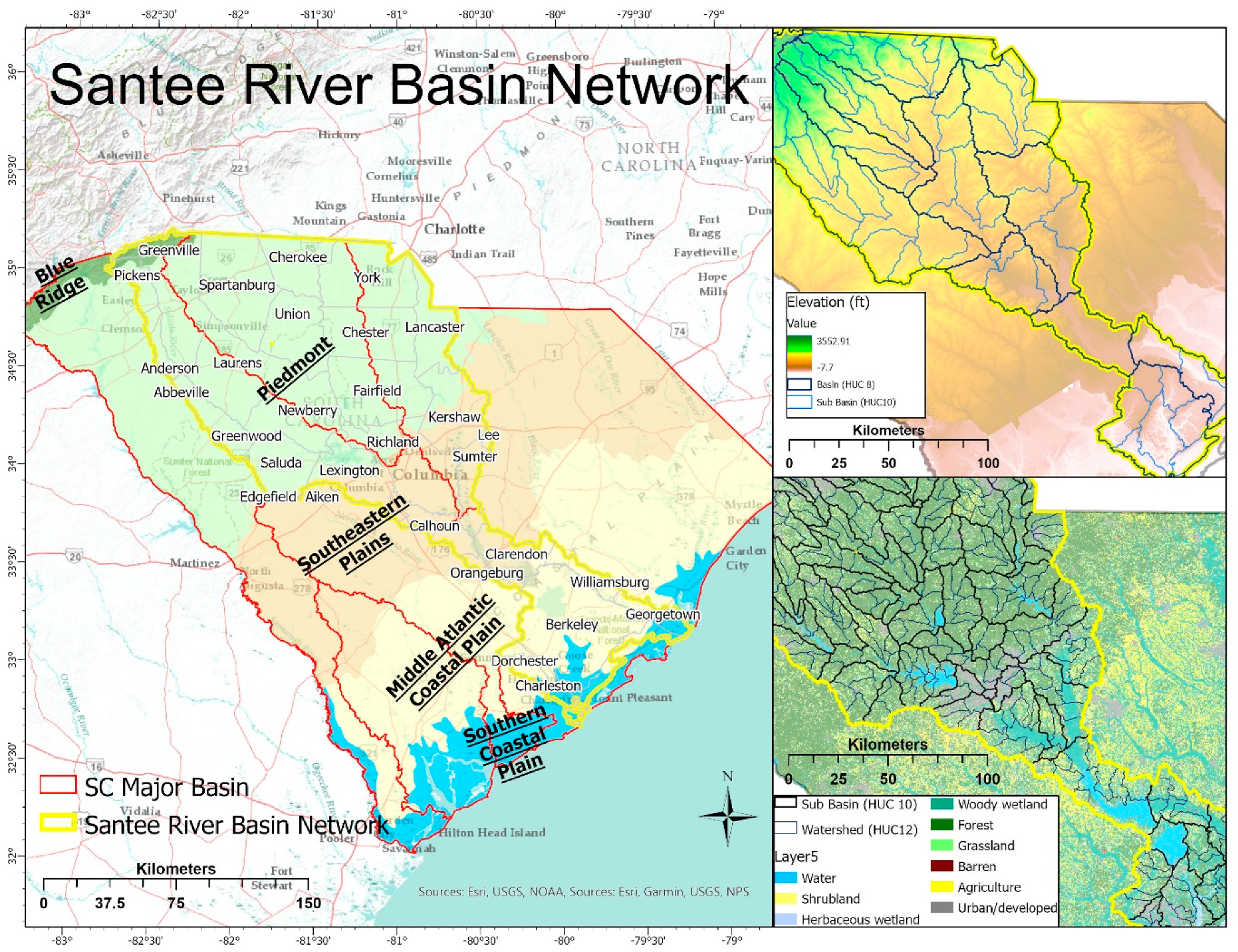
The Santee River Basin Network (SRBN) is a major river basin network in South Carolina (SC) (Figure 1). It originates from the mountains in southern North Carolina and traverses the upstate South Carolina to the coast [36]. The majority of the SRBN’s land cover is classified as vegetated, with forest land covering 51% of the landscape; wetland covers 12%, grassland 11%, shrubland and agriculture 8%, water bodies 4%, developed or urban areas covering 14% and barren land at less than 1% of the total landscape [37]. The SRBN is a 7.54 million-acre network of river basins and is further subdivided into four major basins: Broad, Catawba, Saluda and Santee-Cooper. The SRBN landscape hosts approximately 79% of SC’s total population across 30 counties [38]. The basin is home to 3.5 million people with a concentration of residents in major cities such as Charlotte, N.C., Greenville-Spartanburg, Columbia and Charleston, S.C. South Carolina has become a popular place to relocate, own a second home, or invest in real estate. As urban areas continue to grow, changing land cover from forested and agriculture to urban and developed land also increases. This change in land use affects the provision of ES in SRBN. For example, growing residential areas and urban land also increases the use of pesticides and fertilizers on lawns and landscapes, as well as the area covered by impervious surfaces. This increases the possibility of flooding and the transportation of contaminants through runoff, ultimately degrading water quality [36].
This paper investigated the contribution of different land cover to the provision of water quality related ES within the SRBN using InVEST. We used the Sediment Delivery Ratio and Water Yield models of the InVEST package to quantify the amount of sediments retained and potential water yield across the landscape. Through the combined results of these models, we were able to identify which land cover provides more ES benefits in terms of water quality regulation. Moreover, we also estimated the per unit area ES contribution by land cover type. The study hypothesized that different land cover types, combined with climate factors, directly impact the quality and quantity of water. Therefore, each land cover type has a different capacity to provide water-related ES. Specifically, following the previous studies [39,40,41], we hypothesized that vegetated areas provide higher ES compared to non-vegetated areas. Alternatively, increasing urbanized and non-vegetated areas decreases the ES provision.
2. Materials and Methods
2.1. Sediment Delivery Ratio (SDR) Model
The InVEST Sediment Delivery Ratio (SDR) model estimates the amount of sediments being exported to the streams and retained by the land cover within a watershed boundary. It computes for the amount of sediment exported and the ratio being retained on a pixel scale level. The model assumes that sediments go to the stream, regardless of location and will eventually reach the end of the stream [42]. Hence, we can evaluate the total sediment being exported by the landscape and can be sorted by land cover type contribution.
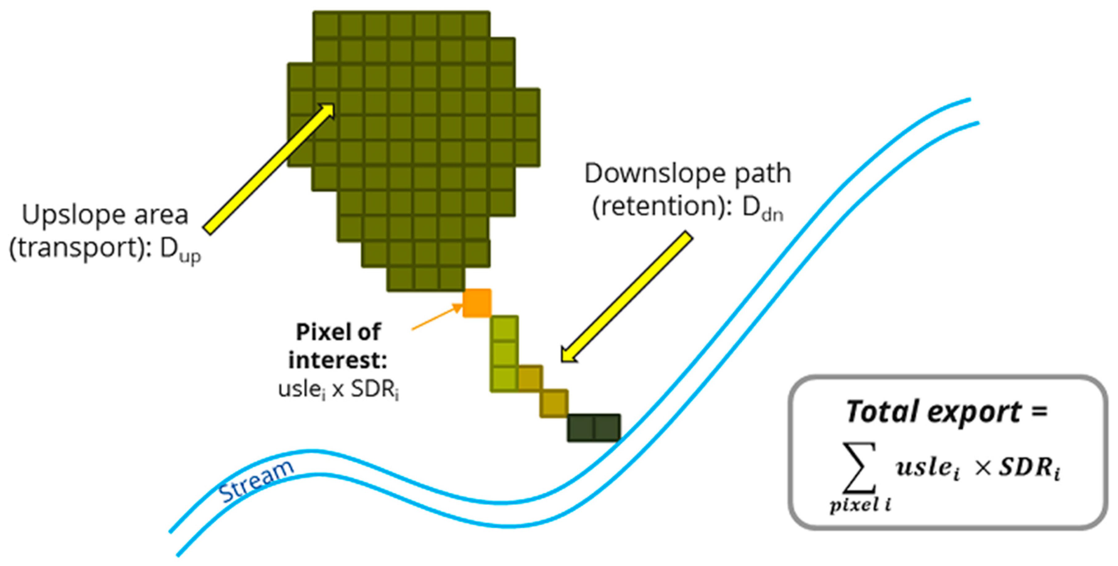
To compute for the Sediment Export, the SDR uses the Revised Universal Soil Loss Equation (RUSLE) and a sediment delivery ratio (SDRi) factor to estimate the amount of sediments contributed by each pixel (Figure 2).
The USLEi computes for the total sediment export per pixel as a function of rainfall erosivity (Ri), soil erodibility (Ki), slope length-gradient factor (LSi), crop-management factor (Ci) and support practice factor (Pi) [34]. This equation is widely used and accepted for estimating soil loss. The SDR factor for each pixel is a function of the connectivity index (IC) [9] which is affected by upslope factors, represented by Dup [10] and downslope factors, represented by Ddn [11]. The InVEST SDR model follows the original approach developed by Borselli et al. (2008) in applying the RUSLE. The SDR model’s main improvement is that it considers the hydrologic connectivity and land cover changes within the landscape in estimating the total amount of sediments being exported to the streams. Furthermore, this is possible by using parameters IC0 and kb, which define the relationship between the connectivity index and the SDR [34]. Therefore, the SDR model estimates the amount of sediment being exported to the stream considering the current land cover.
A byproduct of the SDR model is an estimate of the total sediment exported in a scenario where the land cover are not considered, also known as a bare ground scenario. Therefore, while the SDR model focuses on estimating the sediments being exported to the stream, this can also be used to compute the amount of sediment being retained by the land cover. The difference between the sediment export with the land cover and the sediment export with the bare ground scenario, results in the amount of sediments retained by the land cover. This contributes to the water quality regulation which was the focus of this study.
2.2. Water Yield (WY) Model
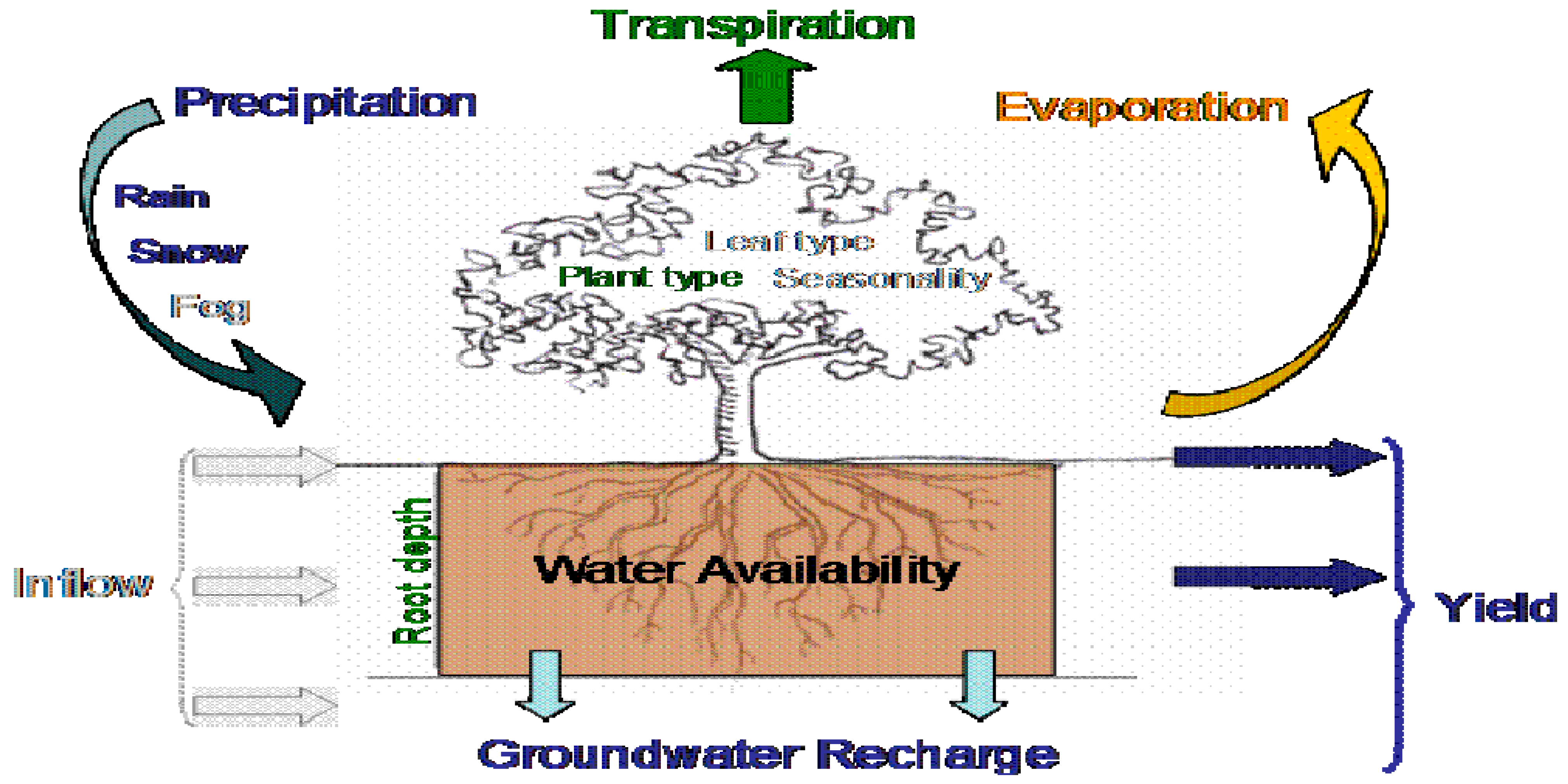
The InVEST Water Yield (WY) model is the module for estimating the potential volume of water that a land cover can capture from rain events. While the model is originally intended for hydropower production, the information for quantifying the amount of water is still useful for analyzing the land cover contribution to surface water [34,43].
The WY model framework (Figure 3) is based on the Budyko curve and average precipitation to estimate the amount of potential water yield per pixel [34]. The model estimates the actual evapotranspiration, AET(x) and subtracts it from the total amount of water from precipitation, P(x), that a pixel receives. The AET is derived based on the Budyko curve [44,45] using the parameters potential evapotranspiration, PET(x) and w(x), which is a non-physical parameter for climatic-soil properties [34]. The w(x) is a function of the volumetric plant available water capacity of the soil, AWC(x); the average precipitation, P(x); and an empirical constant Z which captures the local precipitation pattern and hydrogeological characteristics [34,43,46].
The WY model estimates can provide different information about the landscape’s water yield potential. Depending on the spatial scale of the analysis, the estimates can be interpreted differently. For example, estimating the total water yield that can be gathered by the overall area can be interpreted as the potential contribution of the landscape to the water supply. Therefore, a higher overall water yield potential will result in a benefit and an improvement of the ES [46,47]. However, if the WY potential estimate is assessed per land cover or per unit area, the amount of water that each pixel retained after a rain event is expected to be released to the streams through surface runoff [34,39,41,48]. Hence, a higher WY potential per unit area will indicate a higher likelihood of surface runoff. Consequently, in a per area and per land cover analysis, a lower WY potential will indicate in a lower possibility of surface runoff, thus implying an improvement of ES.
2.3. Data Requirements
The data requirements of the InVEST models are mainly spatially explicit files and a tabular dataset that corresponds to the biophysical characteristics per land cover. Table 1 lists the details of the data inputs for the SDR and WY models.
Since the output of the InVEST model is highly dependent on the resolution of the inputs, particularly of the DEM, we used a LiDAR-based DEM of South Carolina counties with a resolution of 3 m × 3 m per pixel mosaiced into a state DEM [49]. The DEM sets the standard for the pixel resolution of the InVEST model’s output [34]. For models that do not require the DEM, the land cover raster file was the secondary basis of the output resolution [34]. Since both models used the land cover files, we resampled the land cover file into 9 m × 9 m pixel resolution to capture a more accurate analysis of the ES.
For the land cover map raster file, we used the CropScape Cropland Data Layer from the United States Department of Agriculture National Agricultural Statistics Service (USDA-NASS) [37] downloaded from USGS through the National Land Cover Database (NLCD). We utilized the Cropland Data Layer for 2018 to include a detailed breakdown of the agriculture land cover into specific crops. This allowed us to account for crop management factors and support practice factor for the SDR model. For the WY model, we also included a crop coefficient for predicting evapotranspiration [34,56].
Specifically for the SDR model data requirements, the Iso-erosivity map was derived using Renard and Freimund (1994) equation for Coterminous US [50] which was converted from US customary units into metric units (MJ/ha) to adhere to the model specifications [34]. Furthermore, the soil erodibility map, downloaded through ArcGIS Online [51], was also converted into metric units ((tons * ha * hr)/(ha * MJ* mm)) as per model specification [34]. Finally, a comma-separated value (.csv) file containing the crop management factor and support practice factor per land cover was used for the RUSLE computation obtained from the Food and Agriculture Organization (FAO) [56].
For the WY model, the precipitation and reference evapotranspiration raster files were obtained from Climatology Lab [53] and the National Oceanic and Atmospheric Administration (NOAA) [54]. The depth to root restricting layer and plant available water fraction raster files were obtained through the Soil Survey Geographic Database (SSURGO) [55]. Lastly, a comma-separated value (.csv) file containing the crop coefficient (Kc) by land cover was used as a constant multiplier for computing w in the WY model.
All spatial data inputs were delineated using the Hydrologic Unit Classification 12 (HUC 12) obtained from the watershed boundary dataset (WBD) [52] and aggregated as Santee River Basin Network.
2.4. Modifying for Crop Seasonality
One of the limitations of the InVEST model is that it is a single-time analysis. Therefore, it quantifies the ES on an annualized temporal scale using mean values of data inputs. This could be a challenge, particularly for analyzing monthly and seasonal changes to ES. To address this, we ran the InVEST models using parameters that simulated monthly events in the landscape, focusing on the changes in the agriculture land cover.
Using a cropping calendar, we identified which crops are offseason per month. We assumed that the offseason crops will have similar values to idle cropland; hence changing its crop management factor, support practice factor, crop coefficient and its interacting effects with the monthly climate variables. This allowed for quantifying the monthly ES within the SRBN. Furthermore, to account for the effect of the sustainable farming intervention, we ran the models for each month while modifying the crop management factor, support practice factor, and crop coefficient factor of the offseason crops into values based on cover crops.
2.5. Model Limitation and Calibration
The InVEST models are widely applied in the quantification of ES, particularly on a landscape scale [57]. One of its main assets is the model’s spatial characteristics and versatility using GIS as a platform. However, the models are not without their limitation. It can only quantify for a single time period; hence, losing the effect of the temporal changes [35,43,58]. Furthermore, the results of the InVEST model are heavily dependent on the quality of inputs that are used. Inputs with refined spatial resolution yield more accurate and precise results, while coarse spatial resolution datasets are more prone to overestimation and focused more on regional landscape analyses [35,43,59,60,61].
Moreover, there is limited literature that compared the InVEST model results with observed data, making it difficult to validate [46]. The InVEST models simplify the application of hydrology and geomorphology equations on a landscape scale. Depending on the amount of details present in the spatial dataset, the models are prone to standardizing and averaging of parameters across the landscape. This means that the parameters used in one region will be the same across all the regions as long as they are of similar land cover type, which in reality is not true. For example, the crop coefficients of a specific crop can differ between an upland and lowland area. However, due to the standardization of parameters, the model uses the same multiplier on that particular crop regardless of geographic location. Therefore, to address this, the model must be calibrated against actual observed flow and sediment values from monitoring stations [43,57,58].
Finally, for the water yield model, the estimated water yield potential accounts for the total volume of water that can be captured by the land cover [34,41,47]. Part of this volume will infiltrate and contribute to the water supply but a substantial amount will become a runoff [34]. The current WY model does not have the capacity to separate between the volume that infiltrates and becomes a surface runoff. While the aggregated water yield potential across the watershed can be interpreted as a total contribution to water supply, the per unit area estimation can be construed more likely as a surface runoff.
2.6. Calibrating the Model
For calibration purposes, we ran the InVEST models with the same catchment size as the benchmark stations. We adjusted the model parameters until they produced similar quantities as with the benchmark. The actual flow rate readings were used for the WY calibration benchmark, while a sediment deposition estimate [62] was used for the SDR calibration. We based the calibration of the SDR model from the measurement of McCarney-Castle et al. (2017), while the WY model was based on the National Water Information System (NWIS). Both were conducted in the Lawsons Fork Creek, Spartanburg, South Carolina.
The observed annual average sediment yield in Lawsons Fork Creek amounted to 168 tons/km2 [62]. This served as a benchmark to calibrate the InVEST SDR model while adjusting the parameters IC0 and kb. Following the SDR model documentation, we set the IC0 to its default value (0.5) and adjusted the kb parameter [34]. We ran different model iterations using different kb parameter values to produce a closely similar estimate to McCarney-Castle et al. (2017). We determined that a kb value of 0.95–0.96 produced an estimate that was not statistically different from the observed value of McCarney-Castle et al. (2017).
In the same way for the WY model, we used the observed value of 22.53 m/m2/year or a total of 4.3 billion cubic meters per year [63] as a benchmark for calibration. The WY model uses an empirical constant Z, which represents the seasonal distribution of precipitation. We calibrated the Z value by comparing the modeled and observed data to show the sensitivity of the model to the empirical constant [34]. A higher Z value suggests that the sensitivity of the model to the constant is lower [45]. One way to estimate the Z parameter is by multiplying the number of rain events per year to 0.2 constant [40,64]. Therefore, we determined an appropriate Z value of 22 for the Lawsons Fork Creek. In addition, since the WY model is also highly sensitive to variability in precipitation, it is expected that there will be a difference between the observed water yield and the model result [40]. Following the results of the sensitivity analysis, we increased the value of the precipitation data inputs by 9%. Using these calibrated parameters, the model estimated a water yield that was not statistically different from the observed value.
3. Results
3.1. Land Cover Change in SRBN
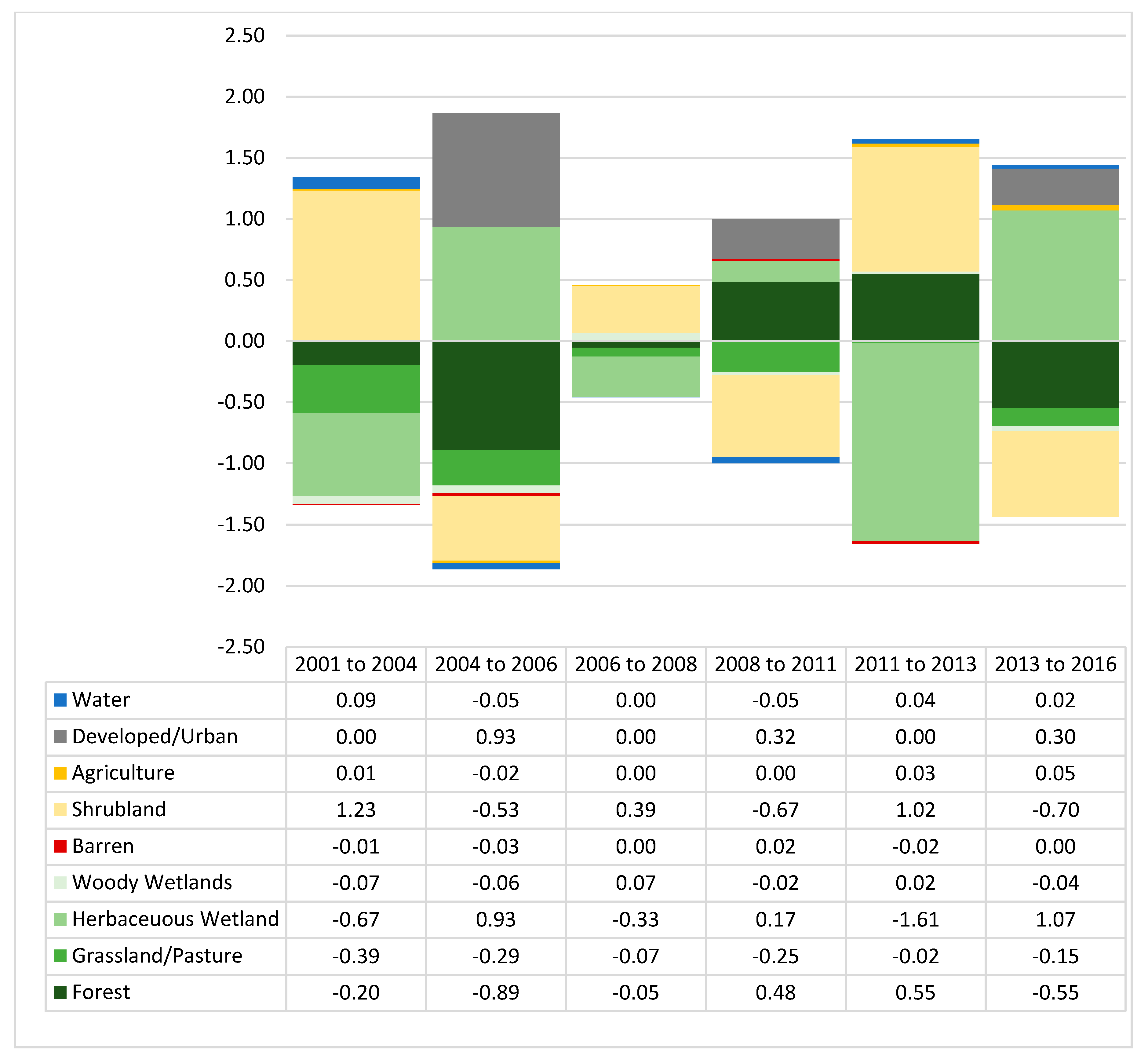
A land cover change analysis between 2016 and 2001 land cover maps (Figure 4) showed that around 200,000 acres (2.5%) of the vegetated land cover in SRBN—including forest land, agriculture, grassland and wetlands—was converted to developed or urban land cover classification [65]. While the percent change of the vegetated land cover seems to be relatively small, the effect on the ecosystems can still be significant.
3.2. Sediment Retention Capacity
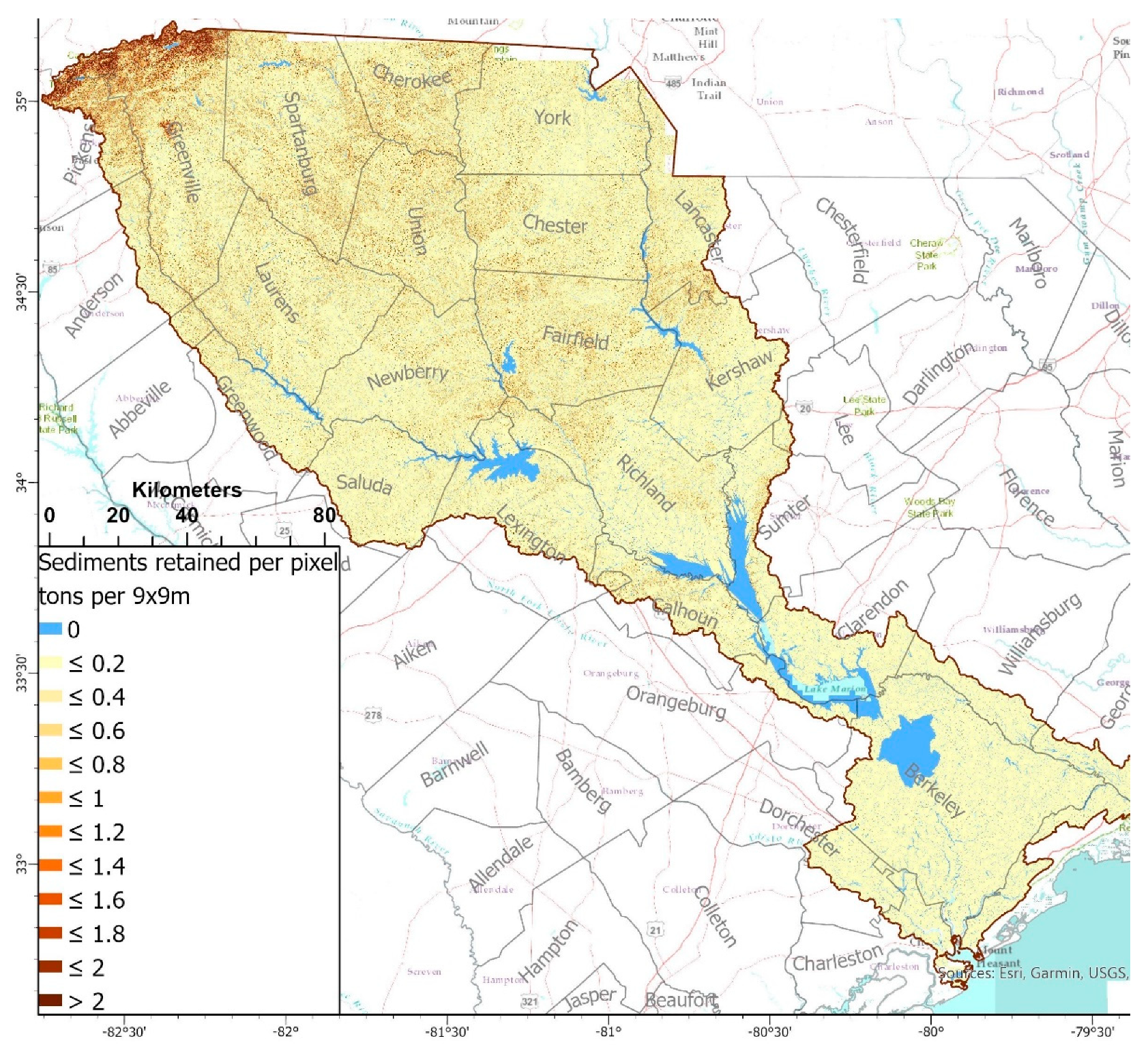
The geographic distribution of the SDR (Figure 5) showed that areas with high sediment retention capacity were mostly located upstream or in the upper regions of the basin. As sediments traveled to lower regions, the amount of sediments being retained decreased. This could be because the land cover upstreams retained and trapped most sediments before reaching the lower regions; hence, fewer sediments were captured in the lower regions.
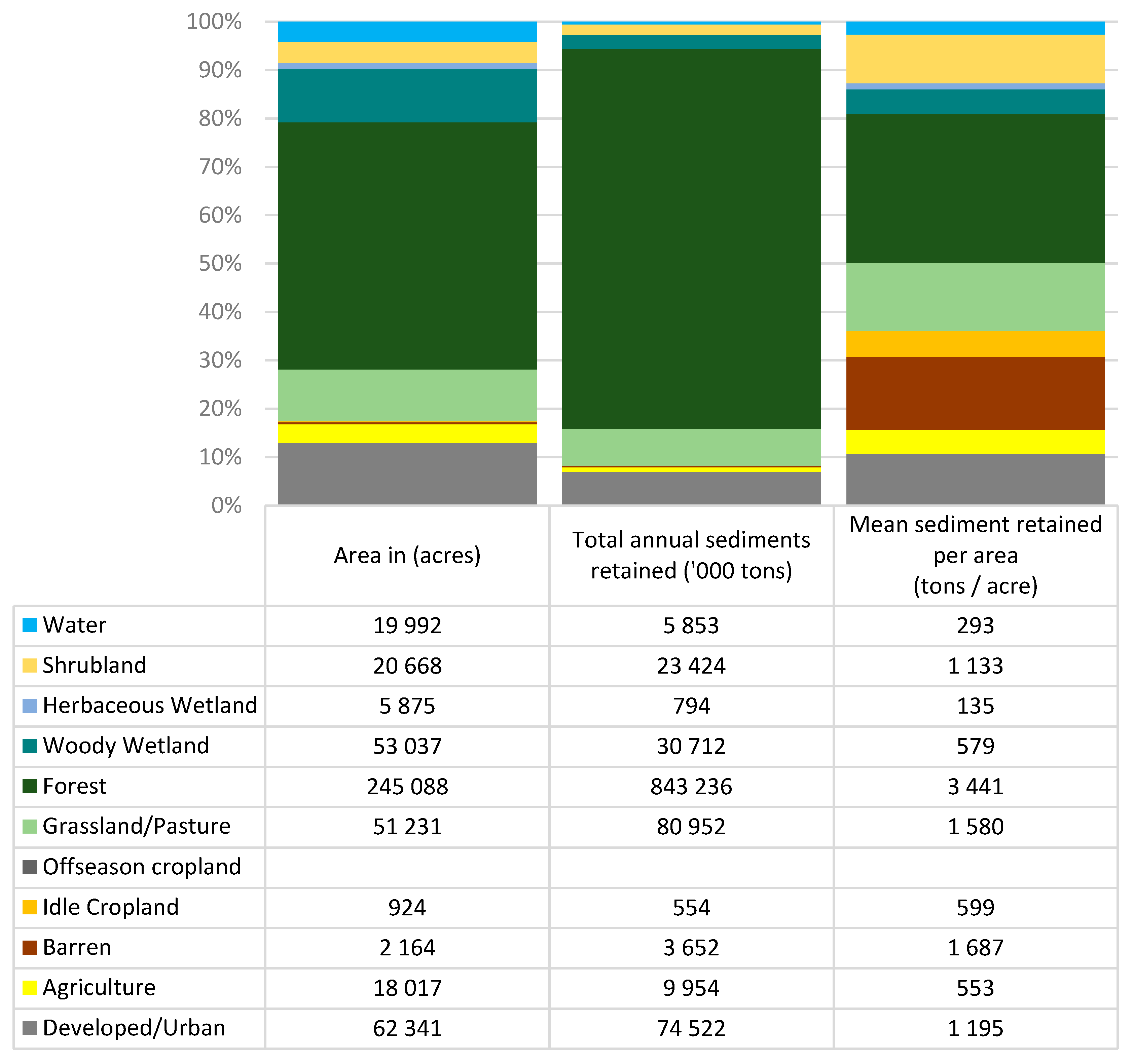
Figure 6 revealed the overall annual sediment retention capacity and the average sediment retention capacity per acre by land. Results showed that forest land cover provided 80% of the overall annual sediment retention ES across the SRBN. Considering that forest land cover is around 50% of the SRBN landscape, this implies that 1% of forest cover across the landscape contributes 1.5% worth of the total sediment retention capacity. The remaining 20% sediment retention provision was split between other vegetated areas—grasslands (7%), woody wetlands (3%), shrublands (2%), and agriculture (1%); and non-vegetated areas—urban (6%) and barren land (1%). This showed that vegetated areas deliver high retention capacity per unit area.
Accounting for Seasonality and the Effect of the Sustainable Farming Intervention to Sediment Retention Capacity
While land cover maps do not change significantly within an annual period, the utilization of some land cover is highly dependent on season, particularly for agricultural land; hence, changing the ES provision every month.
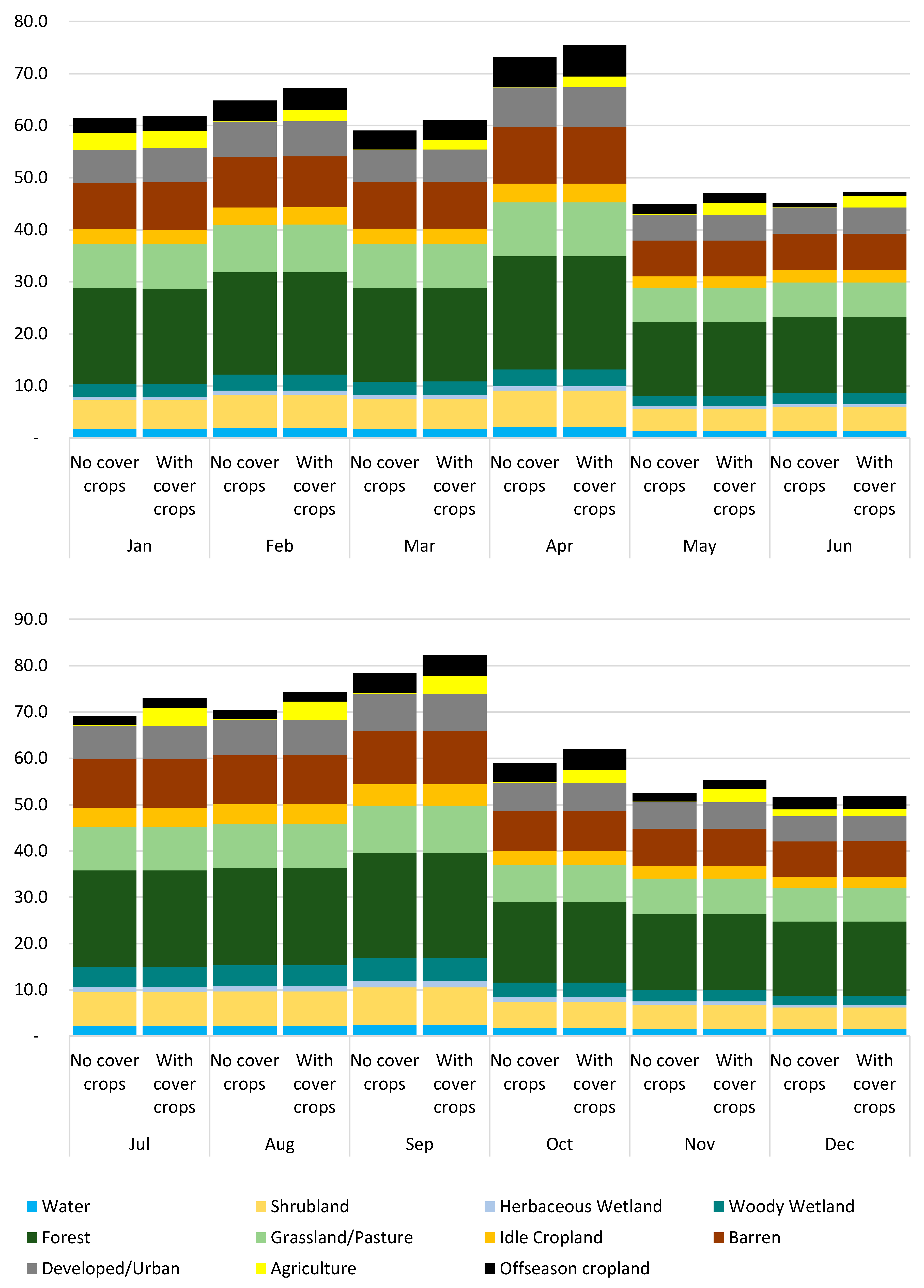
Figure 7 revealed that, if without intervention, areas with offseason crops can have higher sediment retention capacity as compared to agricultural land areas with planted in-season crops. Since the model treated the offseason cropland as idle cropland, the soil characteristics are still compact and permeable due to the regular cropping activities within the area. Furthermore, since the offseason cropland was originally part of the overall agriculture land cover, the cleared area due to the offseason crops created patches of open areas adjacent to other in-season crop areas. These cleared patches tend to hold the sediments that were not retained by the adjacent planted areas.
However, when we assumed that offseason cropland was planted with cover crops, its sediment retention capacity slightly improved. More importantly, the sediment retention capacity of the agriculture land areas increased substantially since patches of open areas were filled. The agricultural land cover improved from a monthly average of 0.5 tons per acre to 2.7 tons per acre. In comparison, the offseason cropland improved from a monthly average of 2.9 tons per acre to 3.1 tons per acre retention capacity with cover crops (Table S1).
3.3. Water Yield Potential
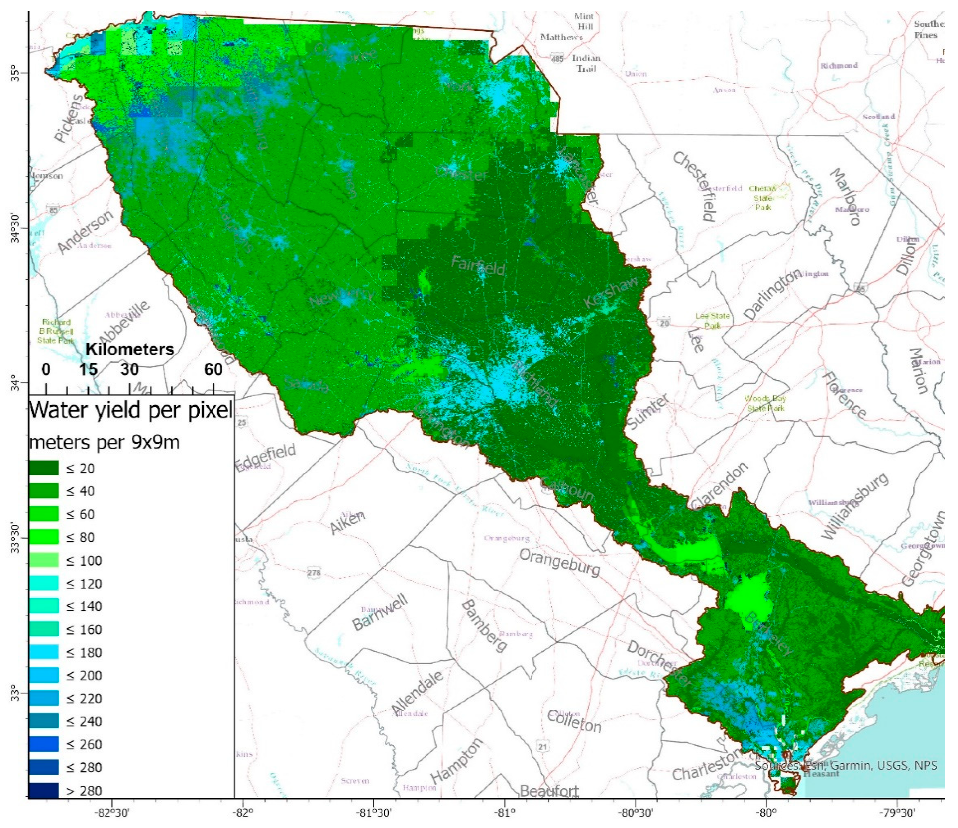
For this study, we focused on the WY potential per area by land cover. This implies that a lower water yield potential is desirable and will improve the water quality regulation. Results showed that the land cover with the highest water yield potential occurred in the upstate region and in some parts of the coastal and midland regions (Figure 8).
The blue areas coincide with the urban/developed areas of the land cover map. This is supported by the results in Figure 9 showing that urban/developed land cover accounted for most (46%) of the estimated total annual water yield potential. However, considering that urban/developed land cover accounted for only 13% of the overall land cover, the ratio of the amount of water yield potential per area was around three times more than a forested land cover area.
Similarly, urban/developed land cover areas had the highest mean water yield potential among the different land cover types. Likewise, other non-vegetated areas such as barren land and idle cropland recorded a high mean water yield potential per area. While these land cover types are not impervious, there is little vegetation that can consume and hold the water.
In contrast, areas with vegetation such as forest, grassland, shrubland and agriculture land cover types dominate the green areas (Figure 8), indicating low water yield potential. Since forest covers majority of the SRBN (Figure 9), it recorded the second highest overall water yield potential (32%). However, the per unit area computation revealed that the forest land has a low water yield potential per pixel. Similarly, other vegetated areas such as wetland, grassland, shrubland and agriculture, also indicated a low water yield potential per unit area.
Accounting for Seasonality and the Effect of the Sustainable Farming Intervention on the Water Yield Potential
The water yield potential is largely affected by evapotranspiration and plants’ water uptake. Since the model accounted for the overall analysis throughout the year, it does not consider the effects brought by the changes from the seasonality of the crops. Therefore, we looked at its impact by running the model on a monthly timeline while using monthly parameters.
Figure 10 showed that without intervention, the offseason cropland has a high amount of mean water yield potential that was almost similar to non-vegetated areas such as barren and idle cropland. With intervention, the monthly water yield potential per unit area of offseason cropland significantly decreased by 83% on the average (Table S2).
Furthermore, the non-vegetated areas (i.e., urban/developed, barren and idle cropland) has the highest water yield potential per unit area, particularly in the upper region, followed by the coastal or low country region and lastly by the midland region. On the other hand, vegetated areas (i.e., forest, grassland, shrubland and agriculture) have low water yield potential per unit area due to the uptake of water by the vegetation.
4. Discussion
The land cover change analysis showed that the land conversion of vegetated areas to non-vegetated areas is continuing. Notably, a substantial amount of forest, wetland and shrubland are being converted into urban/developed areas. A similar pattern was also observed in a land cover analysis of contiguous US from 2001–2011 [66]. These land conversions affect the ecosystems and ES produced within the landscape. Therefore, if the trend of urban areas continuously expands while vegetated areas continue to decline, this can lead to irreversible damage to the ecosystems and their services.
The forest land cover has the highest sediment retention capacity across the landscape. Since forested areas host a diverse composition of plants and trees, this holds together soil organic matter and contributes to the retention of sediments and prevention of soil erosion. Therefore, keeping the forest land intact ensures the continuous provision of ES. A similar observation was also found in a previous study about the sediment retention by natural landscapes in the US [67]. This reinforces the need for more forest conservation and management practices such as conservation area development [68,69,70,71], incentivizing ES conservation such as Payments for Ecosystem Services (PES) [72,73,74,75,76] and engaging in carbon markets [77,78,79].
In terms of the mean sediment retention capacity by land cover type, vegetated areas provided higher ES per unit area as compared to non-vegetated areas [67]. By keeping the offseason cropland vegetated with cover crops, the sediments that are originally dispensed by the agricultural land cover are held in place, increasing the agricultural land’s sediment retention capacity. Since both of these areas were initially part of the agricultural land cover, the offseason cropland’s sediment retention capacity is intertwined with the in-season crop areas. Because of spatial continuity, planting cover crops improved the ES provision of both the in-season crop areas and the offseason-cover crop planted areas. Without cover crops to fill in the cleared area patches, the agricultural land captured less sediments. However, with cover crops, offseason crop areas become vegetated, resulting in an improvement in sediment retention capacity for both land cover types.
Retaining sediments within the land area results in better soil erosion control which prevent degradation of rivers and streams [62,80,81]. Additionally, retaining the sediments on the landscape also allows more time for the soil to absorb the nutrients rather than being dispensed to the streams, hence improving soil quality [23,26]. Cover crops provide these services and eventually enhance agricultural land, building back soil organic matter and increasing the viability of agricultural land for both ES and cash crop yields. This suggests that using cover crops as sustainable farming practice improves water quality regulation across the landscape.
In terms of the geographic location, results of the InVEST SDR model showed that the upstate region of SRBN has a high sediment retention capacity. The upstate region has mountainous and densely vegetated areas; therefore, sediments are retained primarily in those areas. Since sediments are captured and trapped in the upstate region, fewer sediment travels downstream, hence expecting lower sediment retention capacity from the lower regions.
When it comes to water yield potential, urban/developed areas recorded the highest estimates among different land cover types. This high potential water yield can be due to the characteristics of the urban land since it has many impervious areas. These areas have low to no evapotranspiration and infiltration capacity; hence, the water yield from these areas will move across the landscape as surface runoff. This result is consistent with the previous studies on the impact of urbanization on surface runoff [66,82].
Similar to non-vegetated areas like idle cropland and barren land cover, urban/developed areas have little or no plant water uptake. Hence, when an agricultural land is not in use such as the case of offseason cropland, its potential water yield per unit area also increases, as well as the possibility of runoff, erosion and sediment export. This will eventually affect the water quality of nearby streams, rivers and other water bodies.
In contrast, vegetated land cover types such as forest, grassland, shrubland and in-season agriculture land recorded low water yield potential per unit area because of the plants’ water uptake. The decrease in the water yield potential per unit area implies a reduction in surface runoff. Since vegetative root systems hold soil in place, the vegetation’s presence also improves soil organic matter within the area. In addition, low runoff implied from a low water yield potential can mean a reduced possibility of flooding. Overall, this improves the water quality of nearby water bodies and enhances soil quality, which ultimately can reduce the farm input costs and improve contribution to flood control [61,83,84]. Therefore, the implementation of cover crops as a sustainable farming practice can improve the ES across the landscape. In contrast, the decline of vegetated land cover can result in decreased ES.
Finally, although the water yield potential per unit area indicates a surface runoff, the overall water yield estimate shows the potential water that can be available for the region. The upstate region of SRBN recorded the highest water yield potential across the landscape. Since most of the headwaters are typically found in this region, it serves as a precipitation catch basin. On the other hand, most streams and rivers eventually converge in coastal areas, thus accumulating a substantial amount of water yield potential for this region. Lastly, the midland region recorded to have the lowest overall water yield estimate.
5. Conclusions
This study quantified the ES, particularly the sediment retention capacity and water yield potential of the different land cover types of the Santee River Basin Network (SRBN). The InVEST Sediment Delivery Ratio (SDR) model was used to estimate the amount of sediments being retained per unit area by each land cover type. Additionally, the InVEST Water Yield (WY) model quantified the potential volume of water yield per unit area. Since the per unit area analysis represents the volume that can be a potential surface runoff, this implies that areas with low water yield generate higher ES.
In both models, results supported the hypothesis that different land cover types provide varying levels of water-related ES. Vegetated areas provide higher ES, particularly the forest land cover type. This means that keeping the forest intact and conserved is critical in continuous ES provision. Also, since areas with offseason cropland perform as idle cropland, monthly changes in agricultural systems that create cleared area patches adversely affect the delivery of ES. This increases landscape susceptibility to erosion and decline in water quality. This finding supports the hypothesis that increasing urbanized and non-vegetated areas decreases the ES provision. In contrast, application of sustainable practices such as planting of cover crops in offseason cropland ensures the continuous provision of the ES. This can eventually translate into cost savings for farmers as it will retain the nutrients needed for planting the next season crops, avoiding unnecessary costs of additional fertilizers.
The study also showed that conservation programs and sustainable farming practices, such as cover crop implementation, provides benefits such as soil health improvement, water quality regulation and continuous provision of water-related ES by keeping the land vegetated. This reinforces the need for more conservation programs and sustainable financing mechanisms to enhance soil conservation in agriculture systems and forest protection, such as the Payments for Ecosystem Services (PES).
The methods applied in this study could potentially be used to design a PES framework within the basin. Since the willingness-to-pay (WTP) or financing support of ES buyers is tied up to the product that they expect to receive [73,76,85,86], quantifying the ES provided by the land cover gives clear information on what ES sellers should deliver. On the other hand, knowing the ES benefits helps the ES sellers choose the appropriate intervention that would maximize the ES. Therefore, quantifying the amount of ES improvement provided by sustainable agricultural practices and conservation programs also estimates the potential value of the benefits of these practices.
Finally, the map of ES generated from this study can provide spatial information about the hotspots of prime areas for ES conservation. For example, integrating the geographic location and the effect of land cover types on ES quantification showed that urban/developed areas in the upper region provided low sediment retention capacity and high water yield potential. This could pose a threat to ecosystem conservation and landscape sustainability planning. However, threats could be mitigated with proper management and conservation of forest land, especially those surrounding the urban/developed land. Furthermore, the quantification of ES can also be used to analyze the effect of sustainable practices on ES delivery. The continuous provision of ES is critical to society’s well-being. Therefore, the results of this study can provide inputs and information towards landscape sustainability planning and conservation management practices.
Supplementary Materials
The following are available online at https://0-www-mdpi-com.brum.beds.ac.uk/2073-445X/10/1/21/s1, Table S1: Data of monthly mean sediments retained (tons per acre) by land cover type with and without intervention, Table S2: Data of monthly mean potential water yield (meter per square meter) by land cover type with and without intervention.
Author Contributions
Conceptualization, J.C.U., L.C. and M.M.; methodology, J.C.U.; formal analysis, J.C.U.; investigation, J.C.U. and L.C.; resources, J.C.U. and M.M.; writing—original draft preparation, J.C.U. and L.C.; writing—review and editing, J.C.U., L.C., M.M. and J.U.; visualization, J.C.U. and J.U.; supervision, M.M.; project administration, J.C.U. and M.M.; funding acquisition, M.M. All authors have read and agreed to the published version of the manuscript.
Funding
This research was funded by the National Institute of Food and Agriculture/USDA (Award #: 2018-67020-27854) and the South Carolina Natural Resources Conservation Services (Award #: NR184639XXXXG002).
Institutional Review Board Statement
Not applicable.
Informed Consent Statement
Not applicable.
Data Availability Statement
The data presented in this study are available in the supplementary materials.
Acknowledgments
We acknowledge the reviewers for their comments.
Conflicts of Interest
The authors declare no conflict of interest. The funders had no role in the design of the study; in the collection, analyses or interpretation of data; in the writing of the manuscript or in the decision to publish the results.
References
- Millenium Ecosystem Assessment. Ecosystems and Human Well-Being: Synthesis; Island Press: Washington, DC, USA, 2005. [Google Scholar]
- Kindu, M.; Schneider, T.; Teketay, D.; Knoke, T. Changes of ecosystem service values in response to land use/land cover dynamics in Munessa-Shashemene landscape of the Ethiopian highlands. Sci. Total Environ. 2016, 547, 137–147. [Google Scholar] [CrossRef]
- Hoyer, R.; Chang, H. Assessment of freshwater ecosystem services in the tualatin and Yamhill basins under climate change and urbanization. Appl. Geogr. 2014, 53, 402–416. [Google Scholar] [CrossRef]
- Carpenter, S.R.; Stanley, E.H.; Vander Zanden, M.J. State of the world’s freshwater ecosystems: Physical, chemical, and biological changes. Annu. Rev. Environ. Resour. 2011, 36, 75–99. [Google Scholar] [CrossRef] [Green Version]
- Quintas-Soriano, C.; Castro, A.J.; Castro, H.; García-Llorente, M. Impacts of land use change on ecosystem services and implications for human well-being in Spanish drylands. Land Use Policy 2016, 54, 534–548. [Google Scholar] [CrossRef]
- Foley, J.A. Global Consequences of Land Use. Science 2005, 309, 570–574. [Google Scholar] [CrossRef] [PubMed] [Green Version]
- Lawler, J.J.; Lewis, D.J.; Nelson, E.; Plantinga, A.J.; Polasky, S.; Withey, J.C.; Helmers, D.P.; Martinuzzi, S.; Penningtonh, D.; Radeloff, V.C. Projected land-use change impacts on ecosystem services in the United States. Proc. Natl. Acad. Sci. USA 2014, 111, 7492–7497. [Google Scholar] [CrossRef] [Green Version]
- Kreuter, U.P.; Harris, H.G.; Matlock, M.D.; Lacey, R.E. Change in ecosystem service values in the san antonio area, Texas. Ecol. Econ. 2001, 39, 333–346. [Google Scholar] [CrossRef]
- Krkoška lorencová, E.; Harmáčková, Z.V.; Landová, L.; Pártl, A.; Vačkář, D. Assessing impact of land use and climate change on regulating ecosystem services in the czech republic. Ecosyst. Health Sustain. 2016, 2, e01210. [Google Scholar] [CrossRef]
- Lautenbach, S.; Kugel, C.; Lausch, A.; Seppelt, R. Analysis of historic changes in regional ecosystem service provisioning using land use data. Ecol. Indic. 2011, 11, 676–687. [Google Scholar] [CrossRef]
- Seriño, M.N.; Ureta, J.C.; Baldesco, J.; Galvez, K.J.; Predo, C.; Seriño, E.K. Valuing the Protection Service Provided by Mangroves in Typhoon-hit Areas in the Philippines; EEPSEA Research Report No. 2017-RR19; WorldFish (ICLARM)—Economy and Environment Program for Southeast Asia (EEPSEA): Laguna, Philippines, 2017; ISBN 9786218041523. [Google Scholar]
- Murty, P.L.N.; Sandhya, K.G.; Bhaskaran, P.K.; Jose, F.; Gayathri, R.; Balakrishnan Nair, T.M.; Srinivasa Kumar, T.; Shenoi, S.S.C. A coupled hydrodynamic modeling system for PHAILIN cyclone in the Bay of Bengal. Coast. Eng. 2014, 93, 71–81. [Google Scholar] [CrossRef]
- Tõnisson, H.; Orviku, K.; Jaagus, J.; Suursaar, Ü.; Kont, A.; Rivis, R. Coastal Damages on Saaremaa Island, Estonia, Caused by the Extreme Storm and Flooding on January 9, 2005. J. Coast. Res. 2008, 243, 602–614. [Google Scholar] [CrossRef]
- Abram, N.K.; Meijaard, E.; Ancrenaz, M.; Runting, R.K.; Wells, J.A.; Gaveau, D.; Pellier, A.S.; Mengersen, K. Spatially explicit perceptions of ecosystem services and land cover change in forested regions of Borneo. Ecosyst. Serv. 2014, 7, 116–127. [Google Scholar] [CrossRef] [Green Version]
- Van Reeth, W. Ecosystem Service Indicators: Are We Measuring What We Want to Manage. In Ecosystem Services: Global Issues, Local Practices; Elsevier Inc.: Amsterdam, The Netherlands, 2013; pp. 41–61. [Google Scholar] [CrossRef]
- Wu, J. Landscape sustainability science: Ecosystem services and human well-being in changing landscapes. Landsc. Ecol. 2013, 28, 999–1023. [Google Scholar] [CrossRef]
- Kaspar, T.C.; Singer, J.W. The Use of Cover Crops to Manage Soil. USDA-ARS 2011, 321–337. [Google Scholar] [CrossRef] [Green Version]
- Hoorman, J.J.; Islam, R.; Sundermeier, A.; Reeder, R. Using Cover Crops to Convert to No-Till. Crop. Soils 2009, 42, 9–13. [Google Scholar]
- Mase, A.S.; Gramig, B.M.; Prokopy, L.S. Climate change beliefs, risk perceptions, and adaptation behavior among Midwestern U.S. crop farmers. Clim. Risk Manag. 2017, 15, 8–17. [Google Scholar] [CrossRef]
- Gabriel, J.L.; Garrido, A.; Quemada, M. Cover crops effect on farm benefits and nitrate leaching: Linking economic and environmental analysis. Agric. Syst. 2013, 121, 23–32. [Google Scholar] [CrossRef]
- Reeves, D.W. Cover Crops and Rotations in Crops Residue Management, 1st ed.; CRC Press, Inc.: Boca Raton, FL, USA, 1994; Volume 48, ISBN 9781351071246. [Google Scholar]
- Hobbs, P.R. Conservation Agriculture: What is it and why is it important for future sustainable food production. J. Agric. Sci. 2007, 145, 127–137. [Google Scholar] [CrossRef] [Green Version]
- Fageria, N.K. Role of Soil Organic Matter in Maintaining Sustainability of Cropping Systems. Commun. Soil Sci. Plant Anal. 2012, 43, 2063–2113. [Google Scholar] [CrossRef]
- Pittelkow, C.M.; Liang, X.; Linquist, B.A.; Van Groenigen, L.J.; Lee, J.; Lundy, M.E.; Van Gestel, N.; Six, J.; Venterea, R.T.; Van Kessel, C. Productivity limits and potentials of the principles of conservation agriculture. Nature 2015, 517, 365–368. [Google Scholar] [CrossRef]
- Dunn, M.; Ulrich-Schad, J.D.; Prokopy, L.S.; Myers, R.L.; Watts, C.R.; Scanlon, K. Perceptions and use of cover crops among early adopters: Findings from a national survey. J. Soil Water Conserv. 2016, 71, 29–40. [Google Scholar] [CrossRef]
- Clay, L.; Perkins, K.; Motallebi, M.; Plastina, A.; Farmaha, B.S. The Perceived Benefits, Challenges, and Environmental Effects of Cover Crop Implementation in South Carolina. Agriculture 2020, 10, 372. [Google Scholar] [CrossRef]
- Arbuckle, J.G.; Roesch-McNally, G. Cover crop adoption in Iowa: The role of perceived practice characteristics. J. Soil Water Conserv. 2015, 70, 418–429. [Google Scholar] [CrossRef] [Green Version]
- Liu, S.; Costanza, R.; Troy, A.; D’Aagostino, J.; Mates, W. Valuing New Jersey’s ecosystem services and natural capital: A spatially explicit benefit transfer approach. Environ. Manag. 2010, 45, 1271–1285. [Google Scholar] [CrossRef]
- Costanza, R.; d’Arge, R.; de Groot, R.; Farber, S.; Grasso, M.; Hannon, B.; Limburg, K.; Naeem, S.; O’Neill, R.V.; Paruelo, J.; et al. The value of the world’s ecosystem services and natural capital. Nature 1997, 387, 253–260. [Google Scholar] [CrossRef]
- Schägner, J.P.; Brander, L.; Maes, J.; Hartje, V. Mapping ecosystem services’ values: Current practice and future prospects. Ecosyst. Serv. 2013, 4, 33–46. [Google Scholar] [CrossRef] [Green Version]
- Bateman, I.J.; Harwood, A.R.; Mace, G.M.; Watson, R.T.; Abson, D.J.; Andrews, B.; Binner, A.; Crowe, A.; Day, B.H.; Dugdale, S.; et al. Bringing ecosystem services into economic decision-making: Land use in the United Kingdom. Science 2013, 341, 45–50. [Google Scholar] [CrossRef]
- Wang, Z.; Lechner, A.M.; Baumgartl, T. Mapping cumulative impacts of mining on sediment retention ecosystem service in an Australian mining region. Int. J. Sustain. Dev. World Ecol. 2018, 25, 69–80. [Google Scholar] [CrossRef]
- Bai, Y.; Ochuodho, T.O.; Yang, J. Impact of land use and climate change on water-related ecosystem services in Kentucky, USA. Ecol. Indic. 2019, 102, 51–64. [Google Scholar] [CrossRef]
- Nelson, E.; Ennaanay, D.; Wolny, S.; Olwero, N.; Vigerstol, K.; Penning-ton, D.; Mendoza, G.; Aukema, J.; Foster, J.; Forrest, J.; et al. InVEST 3.6.0 User’s Guide. The Natural Capital Project. 2018, Stanford University, University of Minnesota, The Nature Conservancy, and World Wildlife Fund. Available online: http://data.naturalcapitalproject.org/nightly-build/invest-users-guide/InVEST_3.6.0_Documentation.pdf (accessed on 12 December 2020).
- Sharps, K.; Masante, D.; Thomas, A.; Jackson, B.; Redhead, J.; May, L.; Prosser, H.; Cosby, B.; Emmett, B.; Jones, L. Comparing strengths and weaknesses of three ecosystem services modelling tools in a diverse UK river catchment. Sci. Total Environ. 2017, 584–585, 118–130. [Google Scholar] [CrossRef] [Green Version]
- Hughes, W.B.; Abrahamsen, T.A.; Maluk, T.L.; Reuber, E.J.; Wilhelm, L.J. Water Quality in the Santee River Basin and Coastal Drainages, North and South Carolina, 1995–1998: U.S. Geological Survey Circular 1206. 2000, 32p. Available online: https://pubs.water.usgs.gov/circ1206/ (accessed on 12 December 2020).
- USDA-NASS CropScape—NASS CDL Program. Available online: https://nassgeodata.gmu.edu/CropScape/ (accessed on 26 August 2020).
- United States Census Bureau American Community Survey. Available online: https://data.census.gov/cedsci/table?q=income&t=Income%20%28Households,%20Families,%20Individuals%29&g=0400000US45&tid=ACSST1Y2018.S1901&hidePreview=true (accessed on 23 March 2020).
- Gao, J.; Li, F.; Gao, H.; Zhou, C.; Zhang, X. The impact of land-use change on water-related ecosystem services: A study of the Guishui River Basin, Beijing, China. J. Clean. Prod. 2017, 163, S148–S155. [Google Scholar] [CrossRef]
- Hamel, P.; Guswa, A.J. Uncertainty analysis of a spatially explicit annual water-balance model: Case study of the Cape Fear basin, North Carolina. Hydrol. Earth Syst. Sci. 2015, 19, 839–853. [Google Scholar] [CrossRef] [Green Version]
- Li, S.; Yang, H.; Lacayo, M.; Liu, J.; Lei, G. Impacts of Land-Use and Land-Cover Changes on Water Yield: A Case Study in Jing-Jin-Ji, China. Sustainability 2018, 10, 960. [Google Scholar] [CrossRef] [Green Version]
- Borselli, L.; Cassi, P.; Torri, D. Prolegomena to sediment and flow connectivity in the landscape: A GIS and field numerical assessment. Catena 2008, 75, 268–277. [Google Scholar] [CrossRef]
- Redhead, J.W.; Stratford, C.; Sharps, K.; Jones, L.; Ziv, G.; Clarke, D.; Oliver, T.H.; Bullock, J.M. Empirical validation of the InVEST water yield ecosystem service model at a national scale. Sci. Total Environ. 2016, 569–570, 1418–1426. [Google Scholar] [CrossRef] [PubMed] [Green Version]
- Fu, B.P. On the calculation of the evaporation from land surface. Chin. J. Atmos. Sci. 1981, 5, 23–31. [Google Scholar]
- Zhang, L.; Hickel, K.; Dawes, W.R.; Chiew, F.H.S.; Western, A.W.; Briggs, P.R. A rational function approach for estimating mean annual evapotranspiration. Water Resour. Res. 2004, 40. [Google Scholar] [CrossRef]
- Yang, D.; Liu, W.; Tang, L.; Chen, L.; Li, X.; Xu, X. Estimation of water provision service for monsoon catchments of South China: Applicability of the InVEST model. Landsc. Urban Plan. 2019, 182, 133–143. [Google Scholar] [CrossRef]
- Canqiang, Z.; Wenhua, L.; Biao, Z.; Moucheng, L. Water Yield of Xitiaoxi River Basin Based on InVEST Modeling. J. Resour. Ecol. 2012, 3, 50–54. [Google Scholar] [CrossRef]
- Lang, Y.; Song, W.; Zhang, Y. Responses of the water-yield ecosystem service to climate and land use change in Sancha River Basin, China. Phys. Chem. Earth, Parts A/B/C 2017, 101, 102–111. [Google Scholar] [CrossRef]
- South Carolina Dept of Natural Resources SCDNR—LiDAR Data Status by County. Available online: http://www.dnr.sc.gov/GIS/lidarstatus.html (accessed on 25 June 2019).
- Renard, K.; Freimund, J. Using monthly precipitation data to estimate the R-factor in the revised USLE. J. Hydrology 1994, 157, 287–306. [Google Scholar] [CrossRef]
- ESRI USA Soils Erodibility Factor|ArcGIS Hub. Available online: https://www.arcgis.com/home/item.html?id=ac1bc7c30bd4455e85f01fc51055e586#:~:text=Soil erodibility factor%2C also known,detachment and movement by water (accessed on 19 August 2020).
- USGS National Hydrography Dataset. Available online: https://www.usgs.gov/core-science-systems/ngp/national-hydrography/national-hydrography-dataset?qt-science_support_page_related_con=0#qt-science_support_page_related_con (accessed on 25 June 2019).
- Abatzoglou, J.T. Development of gridded surface meteorological data for ecological applications and modelling. Int. J. Climatol. 2013, 33, 121–131. [Google Scholar] [CrossRef]
- National Weather Service Advanced Hydrologic Prediction Service. Available online: https://water.weather.gov/precip/download.php (accessed on 2 September 2020).
- Soil Survey Staff USDA NRCS Web Soil Survey. Available online: https://websoilsurvey.sc.egov.usda.gov/App/HomePage.htm (accessed on 2 December 2018).
- Allen, R.G.; Pereira, L.S.; Raes, D.; Smith, M. Crop Evapotranspiration: Irrigation and Drainage Paper No. 56. In Food and Agriculture Organization (FAO) of the United Nations; FAO: Rome, Italy, 1998; ISBN 9251042195. [Google Scholar]
- Vigerstol, K.L.; Aukema, J.E. A comparison of tools for modeling freshwater ecosystem services. J. Environ. Manag. 2011, 92, 2403–2409. [Google Scholar] [CrossRef]
- Bagstad, K.J.; Cohen, E.; Ancona, Z.H.; McNulty, S.G.; Sun, G. The sensitivity of ecosystem service models to choices of input data and spatial resolution. Appl. Geogr. 2018, 93, 25–36. [Google Scholar] [CrossRef]
- Bagstad, K.J.; Semmens, D.J.; Winthrop, R. Comparing approaches to spatially explicit ecosystem service modeling: A case study from the San Pedro River, Arizona. Ecosyst. Serv. 2013, 5, 40–50. [Google Scholar] [CrossRef]
- Dennedy-Frank, P.J.; Muenich, R.L.; Chaubey, I.; Ziv, G. Comparing two tools for ecosystem service assessments regarding water resources decisions. J. Environ. Manag. 2016, 177, 331–340. [Google Scholar] [CrossRef] [Green Version]
- Ureta, J.C.; Zurqani, H.A.; Post, C.J.; Ureta, J.; Motallebi, M. Application of Nonhydraulic Delineation Method of Flood Hazard Areas Using LiDAR-Based Data. Geosciences 2020, 10, 338. [Google Scholar] [CrossRef]
- McCarney-Castle, K.; Childress, T.M.; Heaton, C.R. Sediment source identification and load prediction in a mixed-use Piedmont watershed, South Carolina. J. Environ. Manag. 2017, 185, 60–69. [Google Scholar] [CrossRef]
- USGS Surface Water Data for USA: USGS Monthly Statistics. Available online: https://nwis.waterdata.usgs.gov/nwis/monthly?site_no=02156300&por_02156300_125141=2027035,00060,125141,2012-06,2019-10&start_dt=2018-01&end_dt=2018-12&format=html_table&date_format=YYYY-MM-DD&rdb_compression=file&submitted_form (accessed on 11 September 2020).
- Donohue, R.J.; Roderick, M.L.; McVicar, T.R. Roots, storms and soil pores: Incorporating key ecohydrological processes into Budyko’s hydrological model. J. Hydrol. 2012, 436–437, 35–50. [Google Scholar] [CrossRef]
- USGS National Land Cover Database. Available online: https://www.usgs.gov/centers/eros/science/national-land-cover-database?qt-science_center_objects=0#qt-science_center_objects (accessed on 14 September 2020).
- Chen, J.; Theller, L.; Gitau, M.W.; Engel, B.A.; Harbor, J.M. Urbanization impacts on surface runoff of the contiguous United States. J. Environ. Manag. 2017, 187, 470–481. [Google Scholar] [CrossRef]
- Woznicki, S.A.; Cada, P.; Wickham, J.; Schmidt, M.; Baynes, J.; Mehaffey, M.; Neale, A. Sediment retention by natural landscapes in the conterminous United States. Sci. Total Environ. 2020, 745, 140972. [Google Scholar] [CrossRef] [PubMed]
- Lin, Y.-P.; Chen, C.-J.; Lien, W.-Y.; Chang, W.-H.; Petway, J.; Chiang, L.-C. Landscape Conservation Planning to Sustain Ecosystem Services under Climate Change. Sustainability 2019, 11, 1393. [Google Scholar] [CrossRef] [Green Version]
- Chan, K.M.A.; Shaw, M.R.; Cameron, D.R.; Underwood, E.C.; Daily, G.C. Conservation Planning for Ecosystem Services. PLoS Biol. 2006, 4, e379. [Google Scholar] [CrossRef] [PubMed] [Green Version]
- Brown, M.G.; Quinn, J.E. Zoning does not improve the availability of ecosystem services in urban watersheds. A case study from Upstate South Carolina, USA. Ecosyst. Serv. 2018, 34, 254–265. [Google Scholar] [CrossRef]
- Noe, R.R.; Keeler, B.L.; Kilgore, M.A.; Taff, S.J.; Polasky, S. Mainstreaming ecosystem services in state-level conservation planning: Progress and future needs. Ecol. Soc. 2017, 22. [Google Scholar] [CrossRef]
- Grima, N.; Singh, S.J.; Smetschka, B.; Ringhofer, L. Payment for Ecosystem Services (PES) in Latin America: Analysing the performance of 40 case studies. Ecosyst. Serv. 2016, 17, 24–32. [Google Scholar] [CrossRef]
- Thompson, B.S. Institutional challenges for corporate participation in payments for ecosystem services (PES): Insights from Southeast Asia. Sustain. Sci. 2018, 13, 919–935. [Google Scholar] [CrossRef]
- Wunder, S. Revisiting the concept of payments for environmental services. Ecol. Econ. 2015, 117, 234–243. [Google Scholar] [CrossRef]
- Calderon, M.M.; Anit, K.P.A.; Palao, L.K.M.; Lasco, R.D. Households’ Willingness to Pay for Improved Watershed Services of the Layawan Watershed in Oroquieta City, Philippines. J. Sustain. Dev. 2012, 6, 1. [Google Scholar] [CrossRef] [Green Version]
- Ureta, J.C.P.; Lasco, R.D.; Sajise, A.J.U.; Calderon, M.M. A ridge-to-reef ecosystem-based valuation approach to biodiversity conservation in Layawan Watershed, Misamis Occidental, Philippines. J. Environ. Sci. Manag. 2016, 19, 64–75. [Google Scholar]
- Clay, L.; Motallebi, M.; Song, B. An Analysis of Common Forest Management Practices for Carbon Sequestration in South Carolina. Forests 2019, 10, 949. [Google Scholar] [CrossRef] [Green Version]
- Campbell, E.T.; Tilley, D.R. Valuing ecosystem services from Maryland forests using environmental accounting. Ecosyst. Serv. 2014, 7, 141–151. [Google Scholar] [CrossRef]
- Wood, A.; Tolera, M.; Snell, M.; O’Hara, P.; Hailu, A. Community forest management (CFM) in south-west Ethiopia: Maintaining forests, biodiversity and carbon stocks to support wild coffee conservation. Glob. Environ. Chang. 2019, 59, 101980. [Google Scholar] [CrossRef]
- Bracken, L.J.; Turnbull, L.; Wainwright, J.; Bogaart, P. Sediment connectivity: A framework for understanding sediment transfer at multiple scales. Earth Surf. Process. Landforms 2015, 40, 177–188. [Google Scholar] [CrossRef] [Green Version]
- Osouli, A.; Bloorchian, A.A.; Nassiri, S.; Marlow, S. Effect of Sediment Accumulation on Best Management Practice (BMP) Stormwater Runoff Volume Reduction Performance for Roadways. Water 2017, 9, 980. [Google Scholar] [CrossRef] [Green Version]
- Hung, C.L.J.; James, L.A.; Carbone, G.J. Impacts of urbanization on stormflow magnitudes in small catchments in the Sandhills of South Carolina, USA. Anthropocene 2018, 23, 17–28. [Google Scholar] [CrossRef]
- Ward, J.V.; Tockner, K.; Schiemer, F. Biodiversity of Floodplain River Ecosystems: Ecotones. Regul. Rivers Res. Manag. 1999, 15, 125–139. [Google Scholar] [CrossRef]
- Zurqani, H.A.; Post, C.J.; Mikhailova, E.A.; Cope, M.P.; Allen, J.S.; Lytle, B.A. Evaluating the integrity of forested riparian buffers over a large area using LiDAR data and Google Earth Engine. Sci. Rep. 2020, 10, 14096. [Google Scholar] [CrossRef]
- Mercer, D.E.; Cooley, D.; Hamilton, K. Taking Stock: Payments for Forest Ecosystem Services in the United States. Ecosystem Marketplace. 2011, Forest Trends, Ecosystem Marketplace, US Forest Service. Available online: https://www.fs.usda.gov/treesearch/pubs/38987 (accessed on 12 December 2020).
- Fauzi, A.; Anna, Z. The complexity of the institution of payment for environmental services: A case study of two Indonesian PES schemes. Ecosyst. Serv. 2013, 6, 54–63. [Google Scholar] [CrossRef] [Green Version]
Figure 1.
Santee River Basin Network (SRBN) Study Site.

Figure 2.
The conceptual approach of Integrated Valuation of Ecosystem Services and Tradeoffs (InVEST) Sediment Delivery Ratio (SDR) for calculating the estimated sediment export per pixel. (adapted from InVEST Natural Capital Project) [34].
Figure 2.
The conceptual approach of Integrated Valuation of Ecosystem Services and Tradeoffs (InVEST) Sediment Delivery Ratio (SDR) for calculating the estimated sediment export per pixel. (adapted from InVEST Natural Capital Project) [34].

Figure 3.
Visualization of the InVEST Water Yield (WY) framework for computing water yield potential per pixel (adapted from InVEST Natural Capital Project) [34].
Figure 3.
Visualization of the InVEST Water Yield (WY) framework for computing water yield potential per pixel (adapted from InVEST Natural Capital Project) [34].

Figure 4.
The land cover percent gains/loss shows that vegetated areas such as forest, grassland and herbaceous wetland decreased; while developed/urban areas increased from 2001 to 2016.
Figure 4.
The land cover percent gains/loss shows that vegetated areas such as forest, grassland and herbaceous wetland decreased; while developed/urban areas increased from 2001 to 2016.

Figure 5.
The results of the SDR model showed the geographic distribution of the areas with high and low capacity for sediment retention.
Figure 5.
The results of the SDR model showed the geographic distribution of the areas with high and low capacity for sediment retention.

Figure 6.
The annual total sediments retained per land cover in SRBN showed that the forest land provide the most Scheme 6. Results indicated that forest land cover has the highest retention capacity with a mean of 3400 tons of sediments per acre annually. Furthermore, the overall mean sediments retained per acre of other vegetated areas amounted to 3980 tons per acre, while the non-vegetated areas amounted to 3480 tons per acre.

Figure 7.
Results showed that the mean sediments retained (tons per acre) by land cover type with and without intervention varied per month.
Figure 7.
Results showed that the mean sediments retained (tons per acre) by land cover type with and without intervention varied per month.

Figure 8.
The results of the InVEST WY model showed that the highlighted blue areas have the highest water yield potential per pixel, while the green areas have the lowest.
Figure 8.
The results of the InVEST WY model showed that the highlighted blue areas have the highest water yield potential per pixel, while the green areas have the lowest.

Figure 9.
The urban/developed land cover has the highest annual total water yield potential, while the non-vegetated areas (i.e., developed/urban, barren, idle cropland) recorded the highest mean water yield potential per area.
Figure 9.
The urban/developed land cover has the highest annual total water yield potential, while the non-vegetated areas (i.e., developed/urban, barren, idle cropland) recorded the highest mean water yield potential per area.

Figure 10.
Results showed that the monthly mean water yield potential in meters per square meter with and without cover crops varied per month.
Figure 10.
Results showed that the monthly mean water yield potential in meters per square meter with and without cover crops varied per month.


Table 1.
List of required data inputs for the InVEST models.
| Data | Data Type | Applicable Model | Sources |
|---|---|---|---|
| Digital Elevation Model (DEM) | Raster file (.tif) | SDR | [49] |
| Iso-erosivity map (R factor) | Raster file (.tif) | SDR | [50] |
| Soil erodibility map (K factor) | Raster file (.tif) | SDR | [51] |
| Boundary shapefile (watershed) | Vector file (.shp) | SDR, WY | [52] |
| Land cover map | Raster file (.tif) | SDR, WY | [37] |
| Precipitation | Raster file (.tif) | WY | [53,54] |
| Reference evapotranspiration | Raster file (.tif) | WY | [53,54] |
| Depth to Root Restricting Layer | Raster file (.tif) | WY | [55] |
| Plant available water fraction | Raster file (.tif) | WY | [55] |
| Biophysical table | Non-spatial data matrix (.csv) | SDR, WY | [56] |
Publisher’s Note: MDPI stays neutral with regard to jurisdictional claims in published maps and institutional affiliations. |
© 2020 by the authors. Licensee MDPI, Basel, Switzerland. This article is an open access article distributed under the terms and conditions of the Creative Commons Attribution (CC BY) license (http://creativecommons.org/licenses/by/4.0/).
Share and Cite
MDPI and ACS Style
Ureta, J.C.; Clay, L.; Motallebi, M.; Ureta, J. Quantifying the Landscape’s Ecological Benefits—An Analysis of the Effect of Land Cover Change on Ecosystem Services. Land 2021, 10, 21. https://0-doi-org.brum.beds.ac.uk/10.3390/land10010021
AMA Style
Ureta JC, Clay L, Motallebi M, Ureta J. Quantifying the Landscape’s Ecological Benefits—An Analysis of the Effect of Land Cover Change on Ecosystem Services. Land. 2021; 10(1):21. https://0-doi-org.brum.beds.ac.uk/10.3390/land10010021
Chicago/Turabian StyleUreta, J. Carl, Lucas Clay, Marzieh Motallebi, and Joan Ureta. 2021. "Quantifying the Landscape’s Ecological Benefits—An Analysis of the Effect of Land Cover Change on Ecosystem Services" Land 10, no. 1: 21. https://0-doi-org.brum.beds.ac.uk/10.3390/land10010021
Note that from the first issue of 2016, this journal uses article numbers instead of page numbers. See further details here.