Major United States Land Use as Influenced by an Altering Climate: A Spatial Econometric Approach

Abstract

Climate and socioeconomic and policy factors are found to stimulate land use changes along with changes in greenhouse gas emissions and adaption behaviors. Most of the studies investigating land use changes in the U.S. have not considered potential spatial effects explicitly. We used a two-step linearized multinomial logit to examine the impacts of various factors on conterminous U.S. land use changes including spatial lag coefficients. The estimation results show that the spatial dependences have existed for cropland, pastureland, and grasslands with a negative dependence on forests but weakened in most of the land uses except for croplands. Temperature and precipitation were found to have nonlinear impacts on the land use shares in the succeeding years by exerting opposite effects on crop versus pasture/grass shares. We also predicted land use changes under different climate change scenarios. The simulation results imply that the southern regions of the U.S. would lose cropland shares with further severity under the business-as-usual climate scenarios, while the land use shares for pasture/grass and forest would increase in those regions. As land use plays an important role in the climate system and vice versa, the results from this study may help policymakers tackle climate-driven land use changes and farmers adapt to climate change.

1. Introduction

The relationship between climate and land use has been the subject of a number of studies. These studies indicate that climate and policy factors stimulate human and natural system land use alterations along with changes in net greenhouse gas emissions [1,2,3,4,5,6,7,8,9,10,11,12,13].

Two approaches have been used to link climate change to land use in the literature. The first approach links land use to climate mitigation considering land as both a source and a sink of greenhouse gases. In that setting, land use changes such as deforestation and afforestation can contribute to exacerbation or mitigation of climate change [14]. Studies such as Attwood et al. [15], Lee et al. [16], and U.S. EPA [17] have examined the impact of policies such as carbon sequestration incentives and conservation programs on land use and land practices.

The second approach considers land use changes as a response to climate conditions. Climate change can have impacts on yields of agricultural commodities, land value, water availability, labor supply and health, infrastructure, and environmental quality as well as loss of land due to rising sea levels [18]. Along with natural land cover changes, land use changes can occur in that landowners exposed to such risks can have incentives to change land allocations as an adaptation measure to climate change. Reilly et al. [19] examined the way climate and policy factors influenced agricultural land use and projected changes under future climate change scenarios. Mu et al. [20] and Mu et al. [12] examined land use shifts between cropping and pasture as climate shifts.

We focused on the second approach: climate change impacts on land use changes. Identifying how the climate and non-climate (socio-economic) factors are related to the changes of land uses can be critical for adaptation behaviors of farmers and policies for agriculture and climate change mitigation as compliance with the emissions target of the Paris climate agreement [21].

According to Homer et al. [22], between 2001 and 2016, the conterminous United States experienced changes to about 8% of its land cover, including declines in forest and pasture/hay and grass/shrub, a slight increase in agricultural land, and a persistent increase in developed (urban) land, while pasture/hay mostly transitioned to cultivated crops. Causes of such land changes were found to be varied, including harvests, fire, pests, diseases, and precipitation [22]. The study shows us how US land changed but less how climate and socioeconomic factors affected the changes.

Most studies on land use have not accounted for potential spatial effects, and this in turn may mean that their estimates are biased, as they neglect the fact that there are common factors across space that influence choices [23,24]. Lubowski et al. [25] and Rashford et al. [26] took spatial interrelationships into account, finding that they did significantly alter the estimates, but they did not consider climate change as a driver. Additionally, most previous studies have operated either over large geographic areas relying on aggregate data or have examined small regions using detailed data, but as a consequence, the small region focus precluded inference to broader settings.

This study extends the literature by examining determinants of land use changes in recent years with detailed 10 km × 10 km gridded data while controlling for common forces across proximate regions with spatial econometric methods. For land use, we considered usage as cropland, pastureland, grassland, forest, urban, and other. We also used climate model-based scenarios to project future US land use change.

2. Materials and Methods

2.1. Spatial Issues and Estimation Methods

Conditions and actions in proximate regions are influenced by common factors such as multi-region droughts, major storms, large scale insect outbreaks, similar soil types, and common production systems. Some recent land use studies have controlled for such commonalities [24,27,28] by using spatial econometric methods, taking into consideration correlations in the error terms or between the error terms and independent variables rather than directly including data on the common factors.

In our analysis, following previous studies [4,28], we assumed that a landowner makes a decision to alter land use when the longer-term net returns from an alternative use minus the conversion cost are larger than the net returns from the current land use. We also implicitly built in the relationship between alterations in longer-term climate and profitability and, in turn, land use. In doing that, we assumed that the net returns depend not only on currently observed conditions but also on longer-term, more persistent conditions through lagged values not only in a region but between regions. This assumes that drivers of land usage in an area are longer-term in nature and that the drivers also commonly influence choices in neighboring areas. For example, if farmers employ land uses similar to those also used in nearby regions, they (a) might benefit from lower costs to find labor with needed skills for that land use; (b) might react to increased incidence of droughts that span across proximate regions; (c) may benefit from needed transport or industrial infrastructure that serves multiple regions; or (d) may employ crop mixes and production systems similar to those in proximate regions that jointly benefit from technological advances and adoption.

Following Li et al. [28], we used an estimation approach that assumes that local land allocation is affected by common factors that also influence land use in nearby regions but do not require one to specify exactly what factors are causing that common influence. In particular, we estimated the probability of each land use considering the allowed uses as cropping, pasture, forest, grass, urban, and other. This was done using a multinomial logit estimator.

The fractional multinomial logit model we estimate that includes in region and spatial lags can be expressed as:

$$\mathrm{E}\left(s_{ijt}|x,w\right)=K_j\left(x_{it-1},w_{ij};\mathsf{\beta },\rho \right)=K\left({{\displaystyle \sum }}_{m\ne i}{\rho }_{jt}{w}_{im}{s}_{mjt}+x_{it-1}{\mathsf{\beta }}_{jt}\right)$$

(1)

where $\mathrm{E}(\cdot )$ tells us the expected probability of land use $j$ in region $i$ during period $t$ as it is influenced by (conditional on) independent variables $x$ and spatial interrelationships $w$. $K(\cdot )$ is the multinomial logit function, ${\rho }_{jt}$ is a spatial interrelationship parameter ($\left|{\rho }_{jt}\right|<1$), implying the degree on which local land use $j$ depends on the use of land use $j$ in nearby areas $m$ as identified by $w_{im}$ times the land uses elsewhere ($s_{mjt})$. The explanatory variables $x$ include physical and socioeconomic factors plus the lagged land use share in the prior time period $t-1$ as a control for potential endogeneity [28]. In the above equation, $w_{im}$ implies the spatial relationship between land areas $i$ and $m$ where, following Li et al. [28], $w_{im}$ has an entry if region $i$ and $m$ are adjacent. By construction, the spatial relation term in a non-adjacent region is 0 ($w_{im}=0,i=m$). The specification in $K(\cdot )$ is often referred to as a spatial lag model [29].

In turn, the conditional mean function is expressed in a matrix form across areas as

$$\mathrm{E}\left(S_{jt}|X,W\right)=K\left({\rho }_{jt}W{S}_{jt}+X_{t-1}{\mathsf{\beta }}_{jt}\right)$$

(2)

where $S_{jt}={\left(s_{1jt},\dots ,s_{Njt}\right)}^{\prime }$ gives land use $j$ proportion across regions 1 through N and $X_{t-1}={\left(x_{1t-1},\dots ,x_{Nt-1}\right)}^{\prime }$ is the set of independent variables in time $t-1$ in each of $N$ regions ($i=1, 2,\dots ,N$). The reduced form of the above equation is $\mathrm{E}\left(S_{jt}|X,W\right)=K\left({\left(I_N-{\rho }_{jt}W\right)}^{-1}{X}_{t-1}{\mathsf{\beta }}_{jt}\right)$, where $I_N$ is an $N$-dimensional identity matrix.

To set up $W$, we follow [29] and use a row-normalized contiguity matrix of first-order neighbors. $W$ is an $N\times N$ matrix where $\sum _{m=1}^N{w}_{im}=1$ and $w_{im}\mathrm{is}\mathrm{nonzero}$ if areas $i$ and $m$ are adjacent and $0$ otherwise.

An important aspect of the spatial lag model is the spatial multiplier, which is estimated by expanding the inverse term in this reduced form: $\mathrm{E}\left(S_{jt}|X,W\right)=K\left(X_{t-1}{\mathsf{\beta }}_{jt}+{\rho }_{jt}W{X}_{t-1}{\mathsf{\beta }}_{jt}+{\rho }_{jt}^2{W}^2{X}_{t-1}{\mathsf{\beta }}_{jt}+\dots \right)$. Thus, the value of $s_{ijt}$ in area $i$ relies not just on prior land use in that area $x_{it-1}$ but also on the uses $x$ in adjacent areas ($-i$), with locations further discounted by powers of ${\rho }_{jt}$. This represents the diminishing nature of the spatial multiplier effects in the spatial lag model. Specifically, if a given explanatory variable $x_{it-1}^k$ changed by one unit in every location, the effect on $s_{ijt}$ would amount to ${\left(1-{\rho }_{jt}\right)}^{-1}{\beta }_{jt}^k$ [30].

Because this nonlinear form of the spatial model can be computationally challenging, especially with the large sample we used, we employed the linearized spatial multinomial logit approach [28,31]. That approach uses the two-step estimation discussed in Appendix A. To perform the spatial estimation, we used a user-written toolbox sparseinv [32] implemented in MATLAB [33] and the matrix technique spmat [34] from Stata [35] that exploits the structure of the contiguity weight matrix. In addition, because it is difficult to interpret the coefficients of such a model due to the nonlinear nature of the logit model and spatial interactions, the partial effects were estimated via a method that is presented in Appendix A.

2.2. Model Specification

Using the above model, we chose the explanatory variables $X_{t-1}$ as previous-year 5-year averages and standard deviations of regional annual mean temperature and precipitation; time-invariant values of elevation, land slope, and land capability class (soil quality); and previous-period values of farm income, non-farm income, population density, and irrigation rate. Climate and geographic variables were also considered as drivers of land use alternative returns, and in turn, land use changes [13,28]. As done in previous studies, incomes, population density, and irrigation rates were used as proxies for factors affecting land values or returns to control for the influence of socioeconomic factors as they vary across counties [36]. The full set of explanatory variables is listed.

All the explanatory variables were lagged 5 years and themselves were 5-year averages, which we felt reflected reactions to not just single-year weather but also longer- term climate characteristics, with the time between observations sufficiently long to allow for land use changes influenced by the explanatory factors.

2.3. Data for Estimation

For our fundamental land use data, we obtained 30×30 m level satellite-based land cover data from the National Land Cover Database (NLCD) of Multi-Resolution Land Characteristics (MRLC) Consortium [22] for the 2001, 2006, 2011, and 2016 periods. The NLCD classifies land cover into many categories, which we aggregated into 6 major use categories following USDA [37]. In particular, we aggregated the categories to cropland, pastureland, grassland, forest, urban, and other [37]. The correspondence between these classifications and the original categories is shown in

Table 1. Matched land use classifications.

Classifications in This Study	NLCD Classifications
Crop	82 (Cultivated Crops)
Pasture	81 (Pasture/Hay)
Forest	41 (Deciduous Forest), 42 (Evergreen Forest), 43 (Mixed Forest)
Grass	71 (Herbaceous), 52 (Shrub/Scrub)
Urban	21 (Developed, Open Space), 22 (Developed, Low Intensity), 23 (Developed, Medium Intensity), 24 (Developed, High Intensity)
Other	11 (Open Water), 12 (Perennial Ice/Snow), 31 (Barren Land), 90 (Woody Wetlands), 95 (Emergent Herbaceous Wetlands)

. Moreover, we needed to aggregate the size of the parcels we considered due to the overwhelming amount of data. Namely, the number of 30 m × 30 m land parcel cells in the US totals nearly 16.8 trillion, so we aggregated to 10 km × 10 km cells, yielding about 80,000 observations per year. Although this prevented capturing the heterogeneity within the 10 km × 10 km cells, it allowed us to capture the interaction between cells.

National-level summaries of land use transitions between 2006 and 2016 are shown in

Table 2. Land use transitions between 2006 and 2016 (thousand km²).

		To
		2016 Land Use
		Crop	Pasture	Grass	Forest	Urban	Other	2006 Total
From 2006 Land Use	Crop	1265.9	1.6	2.3	0.6	3.1	1.6	1275.1
	Pasture	16.6	502.8	2.7	4.8	3.0	1.0	530.9
	Grass	29.2	2.0	2761.4	87.6	4.8	3.7	2888.7
	Forest	0.6	0.9	108.8	1880.3	2.9	0.9	1994.3
	Urban	0.007	0.002	0.001	0.001	413.6	0.001	413.6
	Other	0.9	0.2	3.3	0.5	1.2	970.5	976.7
	2016 Total	1313.1	507.6	2878.5	1973.8	428.6	977.7	8079.3
	Net Change	38.0	−23.3	−20.5	−10.2	15.0	1.0

. In that period, crop and urban land increased while pasture, grass, and forest land decreased, and land in the other categories remained basically unchanged. Unsurprisingly, the data showed that land is most likely to remain in its current use (99.3% for cropland). For cropland, the largest transition out was movement into urban lands, while there were substantial transitions in from pasture and grass. Additionally, note that there were substantial interchanges between grass and forest lands in that period, with the net forest to grasslands conversion adding 20,100 km² to grasslands. The movement into cropland largely from grass and pasture likely was due to price increases under the biofuel boom, while the net forest movement may have been replacing grasslands that moved out to crops.

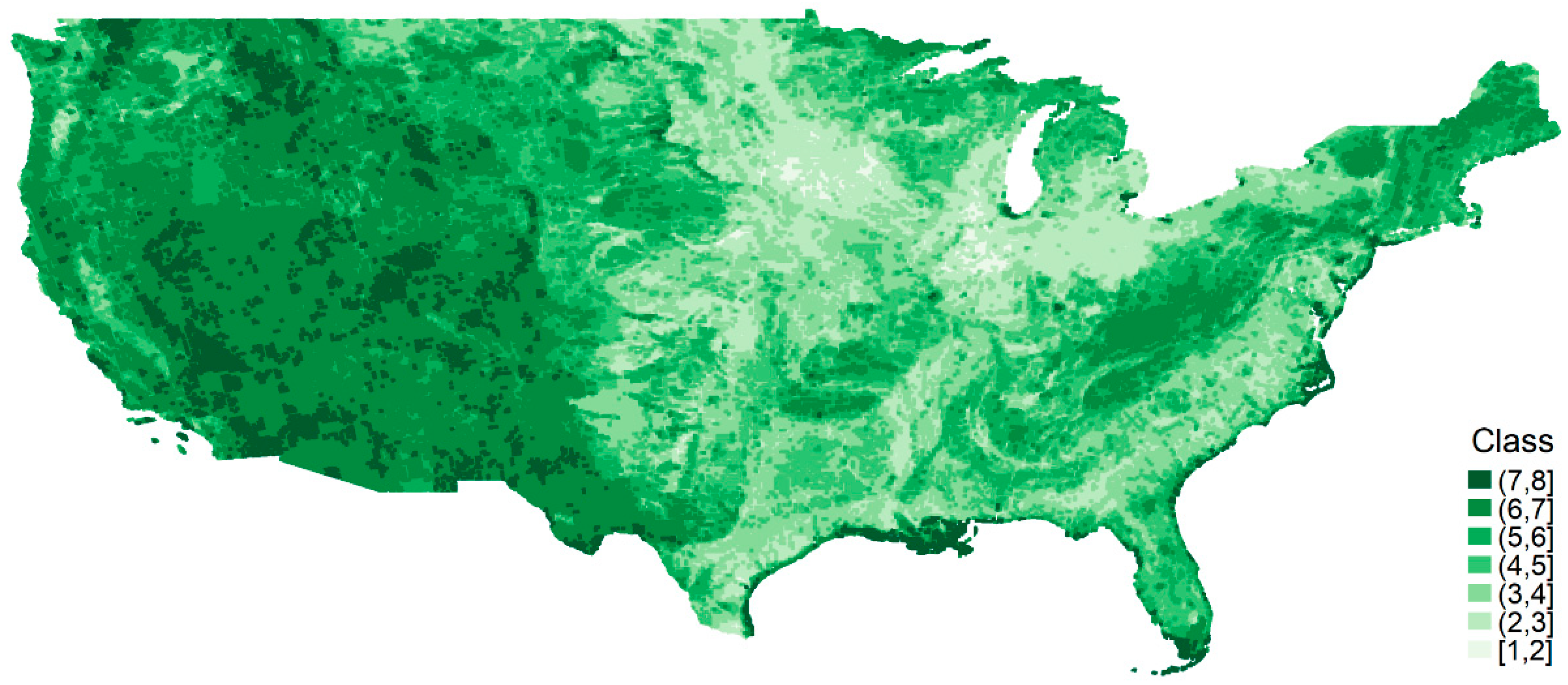
The full set of explanatory variables is listed in

Table 3. Descriptive statistics of explanatory variables (N = 79,657).

Variable	Aggregation	Mean	Std. Dev.	Min.	Max.
Temperature (°C), 2007–2011	10 km × 10 km	11.495	5.265	−2.569	25.631
Temperature (°C), 2012–2016	10 km × 10 km	12.034	5.122	−1.674	26.085
Std. dev. of temperature, 2007–2011	10 km × 10 km	0.809	0.449	0.045	4.627
Std. dev. of temperature, 2012–2016	10 km × 10 km	0.821	0.476	0.042	5.232
Precipitation (m), 2007–2011	10 km × 10 km	0.559	0.176	0.043	1.292
Precipitation (m), 2012–2016	10 km × 10 km	0.910	0.365	0.170	1.981
Std. dev. of precipitation, 2007–2011	10 km × 10 km	0.161	0.105	0.003	0.964
Std. dev. of precipitation, 2012–2016	10 km × 10 km	0.157	0.109	0.004	1.564
Elevation (100 m)	10 km × 10 km	7.683	7.243	−0.741	37.569
Slope (decimal degrees)	10 km × 10 km	0.106	0.110	0.000	0.746
Average LCC for Grid Cell	10 km × 10 km	4.895	1.534	1.383	8.000
Farm income (1000 USD/ha), 2001–2006	County	0.061	0.103	−0.126	0.985
Farm income (1000 USD/ha), 2007–2011	County	0.064	0.123	−0.517	1.042
Nonfarm income (1000 USD/ha), 2001–2006	County	1.314	18.670	0.001	5041
Nonfarm income (1000 USD/ha), 2007–2011	County	1.274	14.132	−7.312	3649
Population density (persons/100 km2), 2001–2006	County	0.344	1.278	0.000	180.212
Population density (persons/100 km2), 2007–2011	County	0.361	1.307	0.000	182.734
Irrigation rate (proportion), 2001–2006	County	0.029	0.068	0.000	0.753
Irrigation rate (proportion), 2007–2011	County	0.029	0.069	0.000	0.711

Notes: Std. Dev. identifies standard deviations. Incomes are adjusted by the gross domestic product deflator to real 2015 USD.

. Elevation, slope, and capability class data were obtained from the USDA Natural Resources Conservation Service soils data base gSSURGO [38]. The land capability classes (LCC) span from class 1 to class 8, with class 1 indicating the land most suitable for cultivation and class 8 the least. Figure 1 presents the capability class data for non-irrigated lands. For ease of interpretation, we converted LCC to a weighted average by 10 km × 10 km grid cell, resulting in a continuous measure between 1 and 8.

The 10 km × 10 km map shown here is a TIGER map [39] portraying the data gridded by using the fishnet function in the ArcGIS software [40].

Climate variables such as annual mean temperature and annual total precipitation were obtained from PRISM [41]. The variables from finer 4 km grids were spatially aggregated to the 10 km × 10 km grid. The mean and standard deviations for the majority of the observations were obtained for a 5-year window.

County-level data for farm and non-farm proprietor income and population estimates were obtained from the U.S. Bureau of Economic Analysis database on Personal Income by County, Metro, and Other Areas [42]. County-level data for irrigated land area were obtained from the USDA Quick Stats database [43]. County-level values for income, population, and irrigation variables were divided by county area, yielding per-hectare values, and were assigned to each grid cell based on the county. When the data for a specific year were not available, the data from a succeeding or preceding year were used.

3. Results

3.1. Estimation Results

We estimated our model as both a linearized spatial multinomial logit and a non-spatial version. The results of that model gave estimates of the probability of a hectare being in a particular use by grid cell, taking into account spatial dependence of the land shares across cells. We estimated land use changes in two different time intervals, one for 2006 to 2011 and the other for 2011 to 2016, then compared differences between those periods.

We found that the coefficient estimates were generally robust between the non-spatial fractional multinomial logit and the spatial version. In terms of choice between the spatial and non-spatial versions, we found that the spatial lag parameter estimates were all positive and significant at the 1% level, except for urban lands (

Table 4. Estimated spatial lag parameters.

	Crop	Pasture	Forest	Grass	Urban
2006–2011	0.031 ***	0.083 ***	−0.018 ***	0.147 ***	0.002 ***
2011–2016	0.050 ***	0.074 ***	−0.020 ***	0.118 ***	−0.001

Notes: *** indicates statistical significance at the 1% level, based on the heteroskedasticity-robust standard errors.

). This implied that the estimates without spatial lag terms could lead to biased estimates [44], and thus, we focused on the spatial estimates in the rest of this paper.

Comparing the results for the period 2001–2006 with those for the period 2006–2011, we found that the cropland share was more influenced by land use patterns in nearby areas in the latter time interval, with pastureland and grassland being less dependent. The spatial dependence terms were mostly significant, excluding those for urban, which likely reflects the fact that allocation to urban lands is largely irreversible. Moreover, the spatial dependence in forestlands was found to be negative. This may be related to the forest fragmentation problem, in which a large forest is segmented into small and sparse forests mostly due to forest loss or distributional changes for other land uses [22,45]. In this case, a large forest may compete with nearby forests and lead to negative spatial dependence on contiguous forest shares. The results differed from those in a China setting [28,46] which found increasing spatial dependence over time. Whether country-specific characteristics affect spatial dependence, or whether other structural changes have occurred should be further investigated.

Table 5. Average partial effects on land use allocations in spatial multinomial logit, 2006–2011.

	Crop	Pasture	Forest	Grass	Urban
Temperature	0.0082 ***	−0.0034 ***	0.0114 ***	−0.0099 ***	0.0037 ***
Temperature squared	−0.0004 ***	0.0001 ***	−0.0004 ***	0.0005 ***	−0.0001 ***
Precipitation	0.0177 ***	0.0186 ***	0.0279 ***	−0.0416 ***	−0.0150 ***
Precipitation squared	−0.0180 ***	−0.0098 ***	−0.0041 ***	0.0186 ***	0.0058 ***
Temperature SD	0.0016	0.0028 **	0.0562 ***	−0.0376 ***	0.0028 **
Precipitation SD	−0.0380 ***	0.0032 *	0.0014	0.0180 ***	−0.0039 **
Elevation	−0.0027 ***	−0.0013 ***	0.0058 ***	0.0005 ***	−0.0006 ***
Slope	−0.0721 ***	0.0386 ***	0.0690 ***	0.0182 ***	0.0395 ***
Land capability class	−0.0057 ***	−0.0013 ***	−0.0044 ***	0.0032 ***	0.0017 ***
Farm income (t − 5)	−0.0057 **	0.0042 **	0.0200 ***	−0.0205 ***	−0.0032 **
Non-farm income (t − 5)	−0.0006 ***	−0.0002 **	0.0003 ***	0.0003 ***	0.0001 ***
log (Pop. density) (t − 5)	−0.0002	0.0014 ***	−0.0001	−0.0041 ***	0.0035 ***
Irrigation rate (t − 5)	0.0547 ***	−0.0415 ***	−0.2171 ***	0.1255 ***	0.0254 ***
Share of crop (t − 5)	0.3001 ***	0.0405 ***	−0.1479 ***	0.0717 ***	0.0240 ***
Share of pasture (t − 5)	0.0879 ***	0.2789 ***	0.0299 ***	−0.1152 ***	0.0165 ***
Share of forest (t − 5)	−0.1113 ***	0.0183 ***	0.3694 ***	0.0649 ***	−0.0158 ***
Share of grass (t − 5)	0.0017	0.0034	−0.1290 ***	0.4397 ***	−0.0180 ***
Share of urban (t − 5)	−0.0049	0.0441 ***	−0.0063	−0.0137 *	0.2284 ***
Observations	79657

Notes: ***, **, and * imply statistical significance at the 1%, 5%, and 10% levels, respectively, based on the standard errors using the delta method.

and

Table 6. Average partial effects on land use allocations in spatial multinomial logit, 2011–2016.

	Crop	Pasture	Forest	Grass	Urban
Temperature	0.0073 ***	−0.0028 ***	0.0079 ***	−0.0080 ***	0.0027 ***
Temperature squared	−0.0004 ***	0.0001 ***	−0.0003 ***	0.0004 ***	−0.0001 ***
Precipitation	0.0149 **	0.0111 **	0.0428 ***	−0.0590 ***	−0.0083 ***
Precipitation squared	−0.0086 **	−0.0062 ***	−0.0084 ***	0.0148 ***	0.0022 ***
Temperature SD	−0.0149 ***	0.0120 ***	0.0157 ***	−0.0109 ***	−0.0021 ***
Precipitation SD	−0.0750 ***	−0.0121 ***	0.0098 ***	0.1044 ***	0.0031 **
Elevation	−0.0032 ***	−0.0008 ***	0.0048 ***	0.0010 ***	−0.0008 ***
Slope	−0.0794 ***	0.0597 ***	0.0395 ***	0.0148 ***	0.0420 ***
Land capability class	−0.0068 ***	−0.0027 ***	−0.0009 **	0.0030 ***	0.0019 ***
Farm income (t − 5)	−0.0166 ***	0.0036 **	0.0274 ***	−0.0127 ***	−0.0021 **
Non-farm income (t − 5)	−0.0008 ***	−0.0002 ***	0.0003 ***	0.0004 ***	0.0001 ***
log (Pop. density) (t − 5)	−0.0001	0.0015 ***	0.0005 **	−0.0049 ***	0.0034 ***
Irrigation rate (t − 5)	0.0560 ***	−0.0440 ***	−0.1992 ***	0.0990 ***	0.0211 ***
Share of crop (t − 5)	0.3036 ***	0.0337 ***	−0.1378 ***	0.0600 ***	0.0273 ***
Share of pasture (t − 5)	0.0957 ***	0.2725 ***	0.0595 ***	−0.1468 ***	0.0167 ***
Share of forest (t − 5)	−0.1185 ***	0.0174 ***	0.3864 ***	0.0532 ***	−0.0154 ***
Share of grass (t − 5)	0.0086 **	−0.0066 **	−0.0999 ***	0.4167 ***	−0.0173 ***
Share of urban (t − 5)	−0.0047	0.0383 ***	0.0146 **	−0.0251 ***	0.2280 ***
Observations	79657

Notes: *** and ** imply statistical significance at the 1% and 5% levels, respectively, based on the standard errors using the delta method.

contain estimates of the average effects of the independent variables on land use change for the intervals 2006–2011 and 2011–2016, respectively. We found that the partial effects of the explanatory variables were mostly consistent across these intervals.

Table 7. Signs and inflection points of nonlinear partial effects of temperature and precipitation on land use allocations, 2011–2016.

	Annual Mean Temperature (°C)			Annual Precipitation (1000 mm)
	Below	Inflection Point	Above	Below	Inflection Point	Above
Crop	+	10.05	−	+	0.86	−
Pasture	−	10.07	+	+	0.89	−
Forest	+	12.16	−	+	2.56	−
Grass	−	10.03	+	−	2.00	+
Urban	+	16.37	−	−	1.89	+

Notes: Entries in the Below and Above columns indicate how the probability of land transfer changes below and above the inflection point. A positive sign (+) in the Below column means the probability of this use increases as temperatures rise toward the inflection point, while a negative in the Above column means the probability falls as temperatures increase above the inflection point. A positive below and a negative above indicates that the probability relation has an inverse U shape, while a negative below and a positive above means the relationship has a U shape.

also shows calculated inflection points for each measure and the signs of the partial effects before and after the inflection points.

The results indicate that higher annual average temperatures above 10 °C led to a decrease in crop and forest lands and an increase in pasture and grasslands. We also found that forest land increased up to an annual average temperature of 12.2 °C and fell above that, while urban land increased up to 16.4 °C and fell thereafter. Collectively, these results for grass and pasture lands reflected a move into crop or forest or urban lands as temperatures increased in areas cooler than the inflection point and movement into grass and pasture lands above that point. The increasing and decreasing effects on crop and forest land-use changes were stronger (with larger magnitudes in quadratic terms) than the effects on urban land-use changes, while the effects from the propensity of grassland to move into other uses were stronger than those for pasture land. Increases in precipitation led to movements into crop, pasture, and forest lands up to the inflection point but decreased thereafter. The opposite effect was seen for grass and urban lands. Larger levels of variation in temperature generally decreased crop, grass, and urban land use but increased that for pasture and forest. For precipitation, greater variation decreased crop and pasture usage but increased that for forest, grass, and urban.

Higher elevations decreased both the crop and pasture shares. This indicated that crop and pasture lands tend to be in lower altitude areas. Land slopes had negative impacts on cropland shares and positive impacts on pasture, forest, and grass. Thus, croplands were more common on flat lands while grazing and forest were favored as slope increased.

Soil quality (in the form of land capability class as it improves moving downward toward 1) positively affected crop, pasture, and forest shares, with the effect greater in the latter time interval for crops and pasture but less for forest. This may indicate that crop and pasture lands were more dependent on land or soil quality between the periods, whereas forests were less dependent.

Increases in the proportion of irrigated land led to greater crop and urban land shares but had negative impacts on pasture, forest, and grasslands. Clearly, more irrigation water supports more land use for crops and also likely indicates available water for urban expansion.

Increases in farm net income decreased crop land use but increased pasture. This may imply that croplands respond more to longer-run asset values but less to short-run annual income, while pasturelands do the opposite.

Non-farm income decreased land use for crops and pasture but increased that for grasslands, forest, and urban lands. This likely reflects greater off-farm commitments and consequent adoption of less labor-intensive forms of land use.

Areas with higher population density increased the incidence of pasture and urban lands but exerted negative impacts on grasslands. This implies that as population grows, grasslands may be converted to pasture or urban lands. It also indicates the pasture lands may be near to urban lands to maintain tax reductions for agricultural land uses involving livestock.

Land use in the previous period positively affected land use in the current period, as we saw in Table 1. Clearly, land allocated for a particular use tends to remain in that use in the next period. However, there are more complex relationships between land uses. Increases in previous forest shares had negative impacts on current cropland shares and vice versa. This may imply that as the region becomes more forested, croplands tend to move into forest lands, but as cropland shares increase, forests are likely to be converted to cropland perhaps due to the incidence of supporting infrastructure. We also found that pastureland and grasslands compete, as pasture decreased when grassland increased or vice versa. This may be because they are competitive as land uses for grazing. We also found that large shares of forests and grasslands in the previous period decreased the probability that land would change to urban use in the current period. This indicates that urban lands are most likely to be developed from crop and pasture lands and less likely to be developed from forest and grasslands.

3.2. Simulation under Climate Scenarios

Using temperature and precipitation estimates from the Representative Concentration Pathways (RCP) of the Coupled Model Intercomparison Project Phase 5 (CMIP5), we applied the model to project land use allocations in 2030, 2050, and 2070. We obtained downscaled projected temperature and precipitation outputs from six climate models: CanESM2, CCSM4, CESM1-CAM5, GFDL-CM3, HadGEM2-ES, and MPI-ESM-MR from the CONUS 1/8 degree BCSD (bias-corrected and spatially downscaled) files available from the Technical Service Center, US Bureau of Reclamation [47]. We use the RCP 2.6 scenario implying optimistic conditions with the lowest level of greenhouse gas emissions, RCP 4.5 scenario deemed as an intermediate scenario, and RCP 8.5 scenario as the hottest scenario. Because we focused on the climate effects on land use changes, we predicted land shares while holding all other variables at current levels. We evaluated the change in shares from the 2016 level.

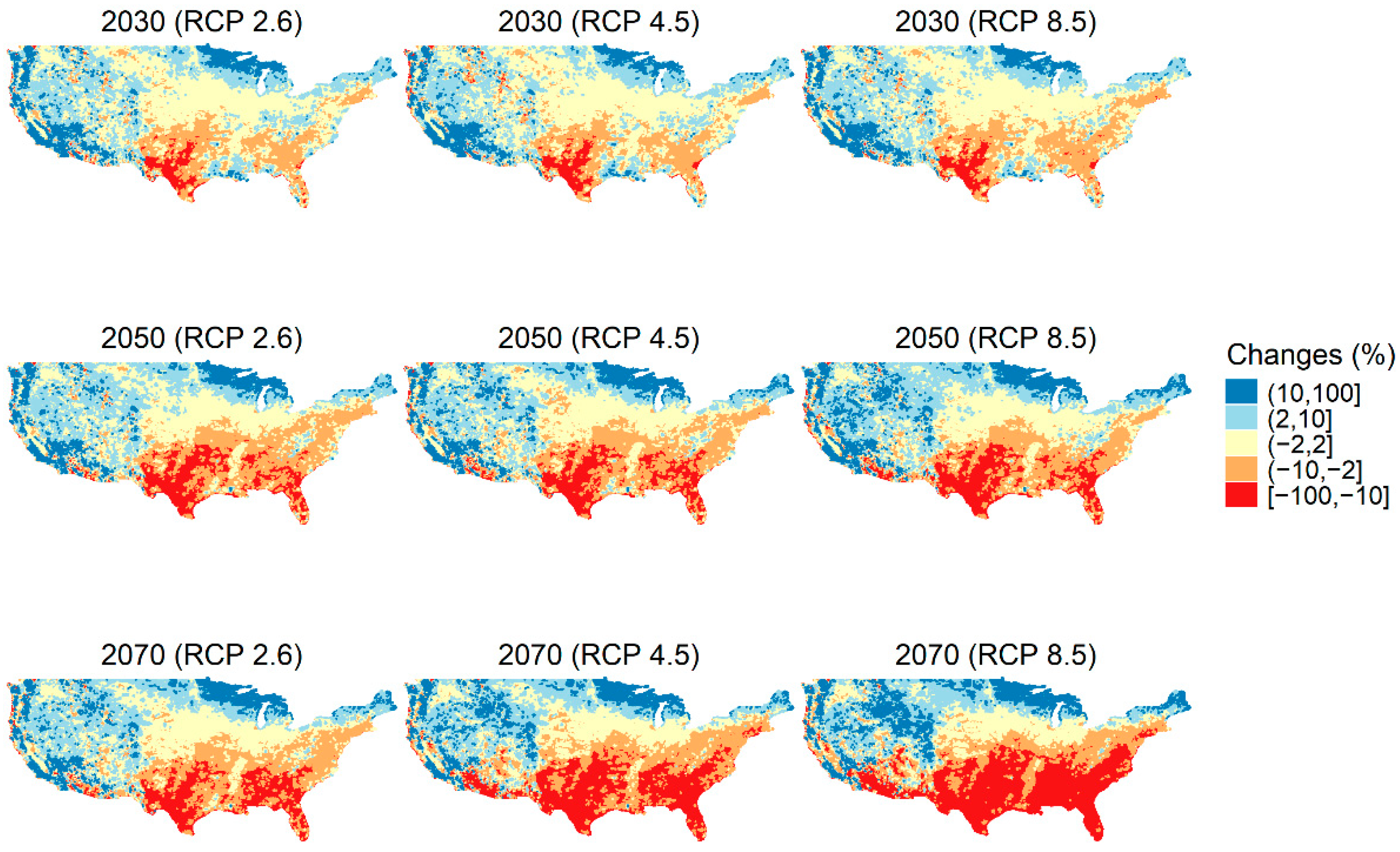
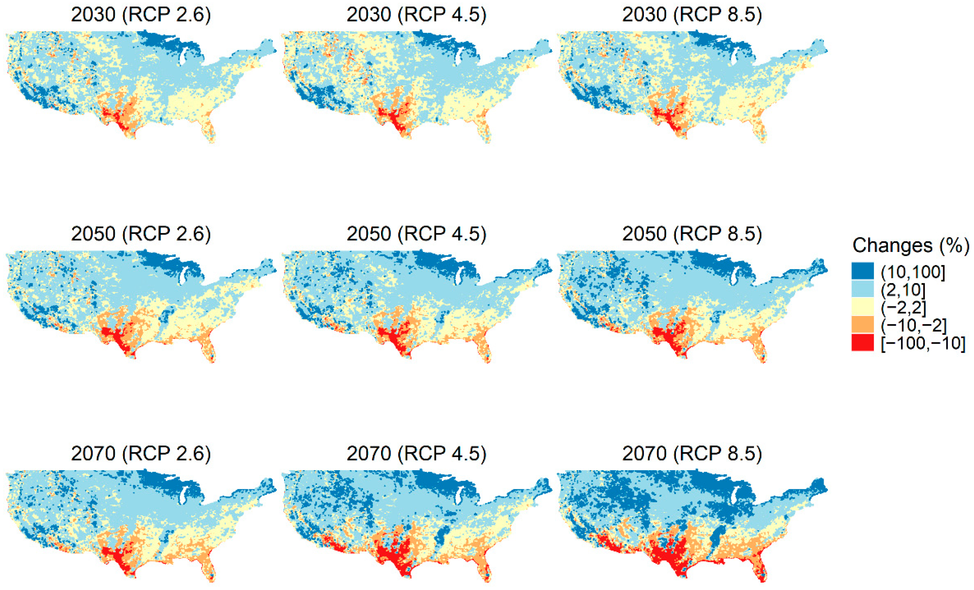
Figure 2 shows the changes in land share for crops under the RCP scenarios. As expected, the RCP 2.6 scenario yielded the least change while RCP 8.5 yielded the largest. In the figure, we see cropland shares decreasing in southern areas and increasing in the Northern, Mountain and Pacific areas.

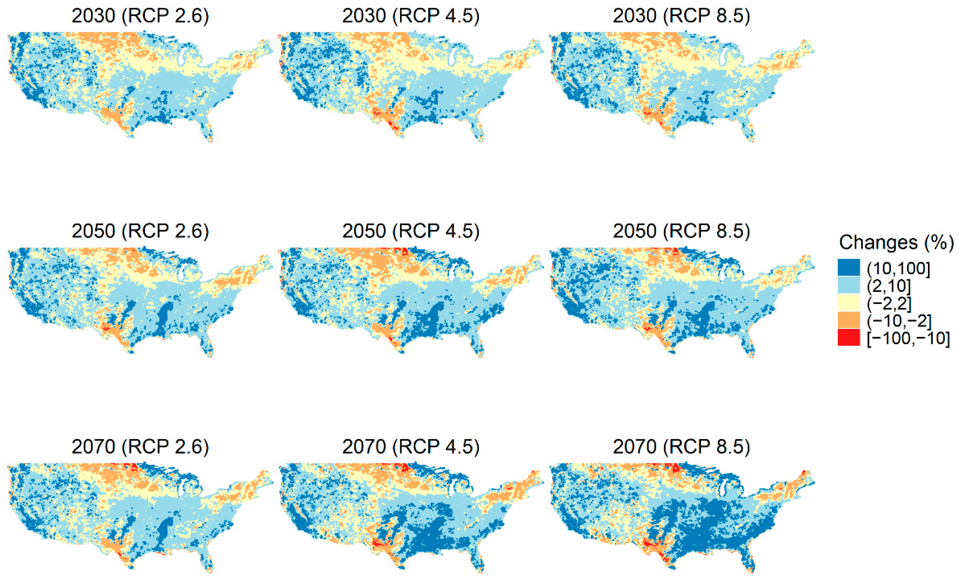
Figure 3 and Figure 4 portray the projected pasture and grassland shares for 2030, 2050, and 2070 compared to 2016. These figures illustrate decreasing shares in the Northern and Midwestern areas, while Southern areas exhibit increasing shares. Again, we see greater sensitivity under RCP 8.5 than under RCP 2.6 or RCP 4.5, particularly in the Midwest. The results for pasture and grass shares are quite similar, reflecting their common use for livestock and the possibility of a rather easy shift between those classifications. This indicates that croplands move into pasture or grass as climate change proceeds.

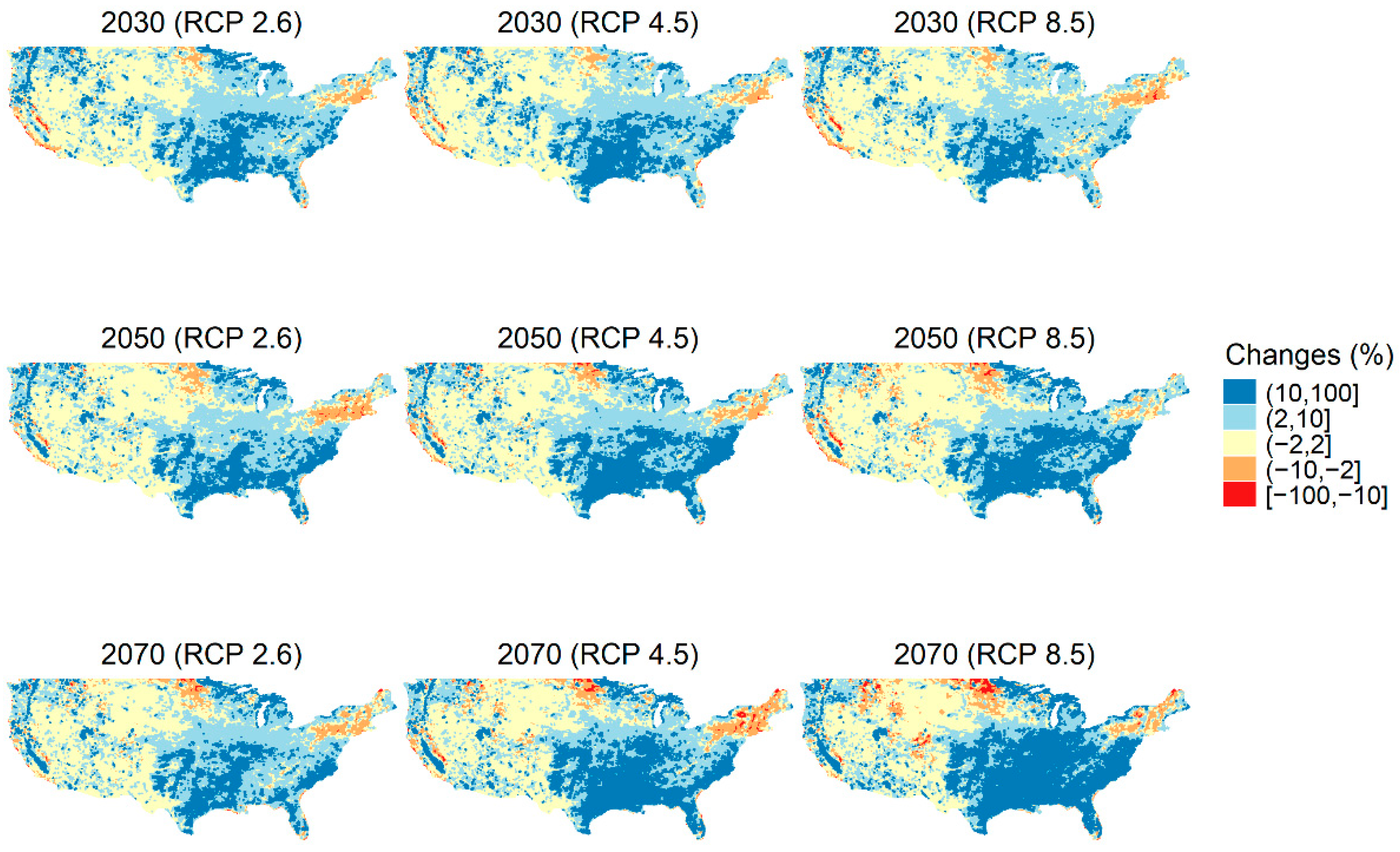
Figure 5 and Figure 6 show projected shares of forest and urban land. In general, they show similar patterns. This may be because the areas with a large share of forest are near more highly developed areas. While both forest and urban land shares decrease in the lower latitudes and increase in the higher latitudes, the increasing forest land share in the Midwestern areas but decreasing shares in the Rocky Mountains likely reflect moisture conditions. The RCP 8.5-based estimates again show greater changes than those for RCP 2.6 or RCP 4.5.

4. Conclusions and Discussion

In the global scheme, the interrelationship between climate change and land use changes has important implications because land plays an important role in both food productivity and land-based emissions. While cropping, livestock, forests, and other land use changes generate about 23% of total greenhouse gas emissions, the Intergovernmental Panel on Climate Change indicates changes in land use and land management can reduce emissions [14]. The land use sector also plays an essential role in supporting multiple Sustainable Development Goals [14]. Given that the US officially rejoined the Paris climate agreement in 2021, changing uses of land, such as curbs on deforestation and the adoption of sustainable land management (SLM), can help achieve emission reductions. However, the climate is also causing changes in land use and may complicate or contribute to mitigation actions.

Herein we reported on a study using US data that examined climate and other factors of influence on land use allocations between five categories of land use. To do this we employed a spatial econometric method—the linearized multinomial logit estimated over fine-scale 10 km × 10 km gridded data. The study approach differed from previous studies in three ways. First, we considered the spatial relationship between nearby areas, whereas other US land use studies mainly ignored it. Second, this study dealt with not just physical factors but also socioeconomic factors influencing land use changes. Third, we utilized fine-scale data to deal with interactions at the grid level. To the best of our knowledge, one or two of these features were shared with some studies but not all three.

Our estimation results implied that spatial dependences importantly influence the shares allocated to most land uses, indicating that estimates omitting them may be biased. This was true for all categories but urban land use, in that case possibly due to irreversibility of that land type. We also found that forestlands showed negative spatial effects, likely because of forest fragmentation. These results may imply that specific land uses likely share common influences with nearby land uses.

The results also show that climate significantly affects land use shares, as do economic and physical conditions. In particular, we found that temperature and precipitation exert opposite yet significant effects on crop versus pasture/grass shares, and that there are also key climate thresholds above which temperature or precipitation causes crop land shares to diminish and pasture/grass shares to increase. This implies that on a local basis, depending on where local conditions fall relative to the threshold, we might see climate change cause either increasing or decreasing cropland shares with countervailing movements in pasture and grasslands. Accordingly, the US ability to mitigate climate change through land use may also be influenced by the extent of climate change and where a region currently stands relative to these thresholds.

Using the estimated model, we projected land use share responses to climate scenarios. We found that climate change generally moves land out of cropping and into pasture or grasslands in the south but increases croplands in the north. This also will requires the attention of policymakers for effective mitigation policy designs. For example, regions with higher shifts into pasture and grassland shares might naturally increase carbon sequestration, whereas those with shifts out of forest land would likely reduce sequestration. Policies could be tuned to regional trends, with those for livestock-supporting uses favoring emissions strategies such as investments in manure management and livestock feeding while those for croplands promote reduced tillage, improved nitrogen fertilizer efficiency, and emission-conserving rice cultivation and other means. Similarly, regions where climate shifts portend less forest may need innovations that improve forest production under changed conditions and species shifts that better accommodate the changed climate. The shifts will also draw attention to regions where crop-based food supplies may diminish and underscore the need for adaptive actions to countervail such forces.

This study also suffered from several limitations. Namely, it omitted factors such as regional policy changes for land uses that merit study despite limited data. Additionally, crop and livestock prices and enterprise-based incomes may be important factors that could be included. Unfortunately, fine-grid scale levels for those types of data are not yet available. For the simulations, our model did not account for feedback from the changed allocations of land.

Future research could improve on this study by including market factors and data across enough time intervals to use a panel spatial model. Additionally, policy factors such as carbon sequestration incentives, carbon prices, and other climate change policies could be explicitly included in the model to allow improved inferences about mitigation policy. Moreover, a comprehensive and global model accounting for land use to climate change feedback integrated with our results would lead to more effective projections and policy recommendations.

References

- Dale, V.H. The relationship between land-use change and climate change. Ecol. Appl. 1997, 7, 753–769. [Google Scholar] [CrossRef]
- Lambin, E.F.; Geist, H.J.; Lepers, E. Dynamics of land-use and land-cover change in tropical regions. Annu. Rev. Environ. Resour. 2003, 28, 205–241. [Google Scholar] [CrossRef] [Green Version]
- Solecki, W.D.; Oliveri, C. Downscaling climate change scenarios in an urban land use change model. J. Environ. Manag. 2004, 72, 105–115. [Google Scholar] [CrossRef] [PubMed]
- Lubowski, R.N.; Plantinga, A.J.; Stavins, R.N. Land-Use change and carbon sinks: Econometric estimation of the carbon sequestration supply function. J. Environ. Econ. Manag. 2006, 51, 135–152. [Google Scholar] [CrossRef] [Green Version]
- Timmins, C. Endogenous land use and the ricardian valuation of climate change. Environ. Resour. Econ. 2006, 33, 119–142. [Google Scholar] [CrossRef]
- Searchinger, T.; Heimlich, R.; Houghton, R.A.; Dong, F.; Elobeid, A.; Fabiosa, J.; Tokgoz, S.; Hayes, D.; Yu, T.H. Use of U.S. croplands for biofuels increases greenhouse gases through emissions from land-use change. Science 2008, 319, 1238–1240. [Google Scholar] [CrossRef] [PubMed]
- Mendelsohn, R.; Dinar, A. Land use and climate change interactions. Annu. Rev. Resour. Econ. 2009, 1, 309–332. [Google Scholar] [CrossRef]
- Hertel, T.W.; Golub, A.A.; Jones, A.D.; O’Hare, M.; Plevin, R.J.; Kammen, D.M. Effects of US Maize ethanol on global land use and greenhouse gas emissions: Estimating market-mediated responses. BioScience 2010, 60, 223–231. [Google Scholar] [CrossRef] [Green Version]
- Plevin, R.J.; O’Hare, M.; Jones, A.D.; Torn, M.S.; Gibbs, H.K. Greenhouse gas emissions from biofuels’ indirect land use change are uncertain but may be much greater than previously estimated. Environ. Sci. Technol. 2010, 44, 8015–8021. [Google Scholar] [CrossRef]
- Alig, R.J. Land use and climate change: A global perspective on mitigation options: Discussion. Am. J. Agric. Econ. 2011, 93, 356–357. [Google Scholar] [CrossRef]
- Haim, D.; Alig, R.J.; Plantinga, A.J.; Sohngen, B. Climate change and future land use in the united states: An Economic approach. Clim. Chang. Econ. 2011, 02, 27–51. [Google Scholar] [CrossRef]
- Mu, J.E.; Wein, A.M.; McCarl, B.A. Land use and management change under climate change adaptation and mitigation strategies: A U.S. case study. Mitig. Adapt. Strateg. Glob. Chang. 2013, 1–14. [Google Scholar] [CrossRef]
- Mu, J.E.; Sleeter, B.M.; Abatzoglou, J.T.; Antle, J.M. Climate impacts on agricultural land use in the USA: The role of socio-economic scenarios. Clim. Chang. 2017, 144, 329–345. [Google Scholar] [CrossRef] [Green Version]
- IPCC Climate Change and Land. An IPCC Special Report on Climate Change, Desertification, Land Degradation, Sustainable Land Management, Food Security, and Greenhouse Gas Fluxes in Terrestrial Ecosystems: Summary for Policymakers; Intergovernmental Panel on Climate Change: Geneva, Switzerland, 2019; ISBN 978-92-9169-154-8. [Google Scholar]
- Attwood, J.D.; McCarl, B.; Chen, C.-C.; Eddleman, B.R.; Nayda, B.; Srinivasan, R. Assessing regional impacts of change: Linking Economic and environmental models. Agric. Syst. 2000, 63, 147–159. [Google Scholar] [CrossRef]
- Lee, H.-C.; McCarl, B.A.; Gillig, D. The dynamic competitiveness of U.S. agricultural and forest carbon sequestration. Can. J. Agric. Econ. 2005, 53, 343–357. [Google Scholar] [CrossRef] [Green Version]
- United States Environmental Protection Agency. Greenhouse Gas. Mitigation Potential in U.S. Forestry and Agriculture; U.S. Environmental Protection Agency: Washington, DC, USA, 2005.
- McCarl, B.A.; Hertel, T.W. Climate Change as an Agricultural Economics Research Topic. Appl. Econ. Perspect. Policy 2018, 40, 60–78. [Google Scholar] [CrossRef]
- Reilly, J.; Tubiello, F.; McCarl, B.; Abler, D.; Darwin, R.; Fuglie, K.; Hollinger, S.; Izaurralde, C.; Jagtap, S.; Jones, J.; et al. U.S. agriculture and climate change: New results. Clim. Chang. 2003, 57, 43–67. [Google Scholar] [CrossRef]
- Mu, J.E.; McCarl, B.A.; Wein, A.M. Adaptation to climate change: Changes in farmland use and stocking rate in the U.S. Mitig. Adapt. Strateg. Glob. Chang. 2013, 18, 713–730. [Google Scholar] [CrossRef] [Green Version]
- Rogelj, J.; den Elzen, M.; Höhne, N.; Fransen, T.; Fekete, H.; Winkler, H.; Schaeffer, R.; Sha, F.; Riahi, K.; Meinshausen, M. Paris agreement climate proposals need a boost to keep warming well below 2 °C. Nature 2016, 534, 631–639. [Google Scholar] [CrossRef] [PubMed] [Green Version]
- Homer, C.; Dewitz, J.; Jin, S.; Xian, G.; Costello, C.; Danielson, P.; Gass, L.; Funk, M.; Wickham, J.; Stehman, S.; et al. Conterminous United States land cover change patterns 2001–2016 from the 2016 national land cover database. ISPRS J. Photogramm. Remote Sens. 2020, 162, 184–199. [Google Scholar] [CrossRef]
- Flores, L.A.; Martinez, L.I.; Ferrer, C.M.; Gallego, V.P.; Bermejo, A.S. A Spatial high-resolution model of the dynamics of agricultural land use. Agric. Econ. 2008, 38, 233–245. [Google Scholar] [CrossRef]
- Chakir, R.; Le Gallo, J. Predicting land use allocation in france: A spatial panel data analysis. Ecol. Econ. 2013, 92, 114–125. [Google Scholar] [CrossRef]
- Lubowski, R.N.; Plantinga, A.J.; Stavins, R.N. What drives land-use change in the United States? A national analysis of landowner decisions. Land Econ. 2008, 84, 529–550. [Google Scholar] [CrossRef]
- Rashford, B.S.; Walker, J.A.; Bastian, C.T. Economics of grassland conversion to cropland in the prairie pothole region. Conserv. Biol. 2011, 25, 276–284. [Google Scholar] [CrossRef]
- Lungarska, A.; Chakir, R. Climate-induced land use change in France: Impacts of agricultural adaptation and climate change mitigation. Ecol. Econ. 2018, 147, 134–154. [Google Scholar] [CrossRef] [Green Version]
- Li, M.; Wu, J.; Deng, X. Identifying drivers of land use change in China: A Spatial multinomial logit model analysis. Land Econ. 2013, 89, 632–654. [Google Scholar] [CrossRef]
- LeSage, J.P. An Introduction to spatial econometrics. Rev. D’économie Ind. 2008, 123, 19–44. [Google Scholar] [CrossRef] [Green Version]
- Kim, C.W.; Phipps, T.T.; Anselin, L. Measuring the Benefits of air quality improvement: A spatial hedonic approach. J. Environ. Econ. Manag. 2003, 45, 24–39. [Google Scholar] [CrossRef] [Green Version]
- Klier, T.; McMillen, D.P. Clustering of auto supplier plants in the united states. J. Bus. Econ. Stat. 2008, 26, 460–471. [Google Scholar] [CrossRef]
- Gilbert, J.R.; Moler, C.; Schreiber, R. Sparse matrices in MATLAB: Design and implementation. Siam J. Matrix Anal. Appl. 1992, 13, 333–356. [Google Scholar] [CrossRef] [Green Version]
- MATLAB. Release 8.3 (R2014a); The MathWorks, Inc.: Natick, MA, USA, 2014. [Google Scholar]
- Drukker, D.M.; Peng, H.; Prucha, I.R.; Raciborski, R. Creating and Managing spatial-weighting matrices with the Spmat command. Stata J. 2013, 13, 242–286. [Google Scholar] [CrossRef] [Green Version]
- StataCorp. Stata Statistical Software: Release 14; StataCorp LP: College Station, TX, USA, 2015. [Google Scholar]
- Deschênes, O.; Greenstone, M. The economic impacts of climate change: Evidence from agricultural output and random fluctuations in weather. Am. Econ. Rev. 2007, 97, 354–385. [Google Scholar] [CrossRef] [Green Version]
- Nickerson, C.; Ebel, R.; Borchers, A.; Carriazo, F. Major Uses of Land in the United States, 2007. Economic Information Bulletin No. (EIB-89); U.S. Department of Agriculture, Economic Research Service: Washington, DC, USA, 2011; p. 55.
- Soil Survey Staff Gridded Soil Survey Geographic (GSSURGO) Database for the Conterminous United States (202007 Official Release); United States Department of Agriculture, Natural Resources Conservation Service: Washington, DC, USA, 2020.
- U.S. Census Bureau. 2008 TIGER/Line Shapefiles (Machine-Readable Data Files); United States Census Bureau: Washington, DC, USA, 2008.
- ESRI. ArcGIS for Desktop: Release 10.2; Environmental Systems Research Institute: Redlands, CA, USA, 2013. [Google Scholar]
- PRISM Climate Group. AN81m Gridded Climate Dataset; Oregon State University: Corvallis, OR, USA, 2019. [Google Scholar]
- U.S. Bureau of Economic Analysis. Personal Income and Employment by Major Component (CAINC4). Available online: https://www.bea.gov/data/income-saving/personal-income-county-metro-and-other-areas (accessed on 2 January 2021).
- USDA National Agricultural Statistics Service. NASS—Quick Stats. Available online: https://data.nal.usda.gov/dataset/nass-quick-stats (accessed on 2 January 2021).
- Pace, R.K.; LeSage, J.P. Omitted Variable Biases of OLS and Spatial Lag Models. In Progress in Spatial Analysis; Páez, A., Gallo, J., Buliung, R.N., Dall’erba, S., Eds.; Advances in Spatial Science; Springer: Berlin/Heidelberg, Germany; Dordrecht, The Netherlands; London, UK; New York, NY, USA, 2010; pp. 17–28. ISBN 978-3-642-03324-7. [Google Scholar]
- Riitters, K.H.; Wickham, J.D.; O’Neill, R.V.; Jones, K.B.; Smith, E.R.; Coulston, J.W.; Wade, T.G.; Smith, J.H. Fragmentation of continental united states forests. Ecosystems 2002, 5, 815–822. [Google Scholar] [CrossRef]
- Zhang, W.-B. Location choice and land use in an isolated state. Ann. Reg. Sci. 1993, 27, 23–39. [Google Scholar] [CrossRef]
- Brekke, L.; Thrasher, B.; Maurer, E.; Pruitt, T. Downscaled CMIP3 and CMIP5 Climate Projections: Release of Downscaled CMIP5 Climate Projections, Comparison with Preceding Information, and Summary of User Needs; Technical Service Center, Bureau of Reclamation, US Department of the Interior: Denver, CO, USA, 2013.
- Cho, S.J. Three Essays on Climate Change Adaptation and Impacts: Econometric Investigations; Texas A&M University: College Station, TX, USA, 2015. [Google Scholar]
- Buis, M.L. FMLOGIT: Stata Module Fitting a Fractional Multinomial Logit Model by Quasi Maximum Likelihood; Boston College Department of Economics: Chestnut Hill, MA, USA, 2008. [Google Scholar]
Figure 1.
Weighted average of land capability classification (non-irrigated). The class values from gSSURGO [38] are averaged at the cell level. Here, lower classes indicate those more suitable for cultivation. Numbers in brackets indicate the range of each category, with the lands in each category having a class greater than the first number and less than or equal to the second one.
Figure 2.
Percentage changes of cropland share between 2016 and select time periods under alternative representative concentration pathways. Numbers in brackets indicate the range of each category, with the change greater than the first number and less or equal to the second one.
Figure 3.
Percentage changes of pastureland share between 2016 and select time periods under alternative representative concentration pathways.
Figure 4.
Percentage changes of grassland share between 2016 and select time periods under alternative representative concentration pathways.
Figure 5.
Percentage changes of forest share between 2016 and select time periods under alternative representative concentration pathways.
Figure 6.
Percentage changes of urban land share between 2016 and select time periods under alternative representative concentration pathways.