The Spatial and Temporal Evolution and Drivers of Habitat Quality in the Hung River Valley

Abstract

The survival and sustainability of regional species is constrained by habitat quality. In recent decades, the intensification of human activities on a global scale has had a profound impact on regional ecosystems and poses a serious threat to regional sustainable development. Scientific measurement of the drivers of habitat quality can provide important support for the development of effective biodiversity conservation and sustainable land-use policies. Taking the Hung River Valley as an example, the InVEST model was used to assess the habitat quality of the study area in 2000, 2005, 2010, 2015, and 2020 and to explore its spatial and temporal variation and distribution characteristics in combination with the spatial autocorrelation model, and the geographically weighted regression (GWR) model was used to explore the drivers of habitat quality change. The results show the following: (1) The overall habitat quality shows an increasing trend during 2000–2020, but the expansion of construction land in the central region plays a dominant role in the degradation of regional habitat quality. (2) The “Guide-Ledu” line is the dividing line of habitat quality in the Hung River Valley, with a general distribution of “south is good, north is bad” and “south is hot, north is cold”. (3) Natural factors such as slope and elevation basically shape the overall distribution pattern of habitat quality, while urbanisation factors such as population density, gross domestic product, and the night-time lighting index are generally negatively correlated with habitat quality. The results of the study can reveal the linkage between ecosystems and land-use change in the context of urbanisation.

1. Introduction

Habitat quality is an important indicator of an ecosystem’s ability to provide suitable conditions for the growth, development, and distribution of species, based on the availability of subsistence resources [1,2]. Since the beginning of industrial society, human activities have caused a series of ecological problems, such as habitat fragmentation and a loss of species diversity, which have led to serious threats to the overall ecological security of the region. In this context, the spatial and temporal distribution characteristics and evolutionary mechanisms of habitat quality have gradually become a hot topic in related research fields [3,4,5,6].

At present, the research on habitat quality in China and abroad has achieved advanced results from macroscopic to microscopic scales. Whether at the local, watershed, or regional scales, scholars have conducted in-depth studies on the spatial and temporal evolution [7], distribution characteristics [8], influencing factors [9,10,11], driving mechanisms [12,13,14,15], and pathways to enhance habitat quality [16,17,18]. Although more research results have been achieved, the current research on the drivers of habitat quality needs to be further explored. There are many factors that influence habitat quality, and the degree of influence of the same influencing factor on habitat quality in different spaces can be spatially heterogeneous [11,19,20]. Simply explaining which influencing factors lead to changes in habitat quality tends to ignore the processes and relationships between subjective and objective elements, which in turn affects the accurate mining of habitat quality influencing factors in the future [21]. Habitat quality is primarily a matter of selecting an evaluation model, and most habitat quality evaluations are based on landscape pattern-based indicator systems and model-based approaches, compared to the more scientific role of models in predicting future habitat distribution and siting protected areas [22,23]. The Integrated Valuation of Environmental Services and Tradeoffs model (InVEST), developed by Stanford University, the World Wildlife Fund, and the Nature Conservancy, has a high data demand. The InVEST (Integrated Valuation of Environmental Services and Tradeoffs) model, developed jointly by the Nature Conservancy and the Nature Fund, has been gradually applied to related studies because of its relatively small data requirements and the high visibility of the results [24,25,26]. In revealing the drivers of habitat quality, ordinary least square (OLS) and geographically weighted regression (GWR) models are good at detecting subtle changes in the process mechanism of habitat quality over time and space, and are an important research method for exploring the drivers of objective objects [27].

The Hung River Valley is in the transition zone between the Qinghai–Tibet Plateau and the Loess Plateau. Its ecological environment is fragile and regarded as a “sensitive area”, and the current literature on the ecology of the region is relatively small [22,23,24]. In the context of the comprehensive pilot work of new urbanisation, the Xining–Haidong metropolitan area will be established in Qinghai Province, and the Hung River Valley area, represented by Xining and Haidong, will usher in a new round of rapid development and become the core growth pole, leading the development of Qinghai and even the northwest region. The development potential brings greater ecological risks. Based on the above research status and regional background, the main research of this paper includes (1) quantitatively assessing the spatial and temporal evolution of the landscape type, landscape pattern, and habitat quality in the Hung River Valley with the help of a land transfer matrix, a landscape pattern analysis method, and the InVEST model; (2) exploring the spatial and temporal coupling relationship between habitat quality change and urbanisation in the Hung River Valley based on the GWR model; (3) finally determining, through the above research, the habitat quality of the Hung River Valley over a 20-year period and the drivers of habitat quality, providing a scientific reference for biodiversity conservation and regional ecological development in the eastern Tibetan Plateau, providing decision support for land use, ecological red line delineation, and coordinated and sustainable economic and social development, and providing new ideas for habitat quality assessments in ecologically sensitive areas.

2. Materials and Methods

2.1. Study Site

The geographical location of the Hung River Valley is 100°51′~103°04′E, 35°01′~38°N (Figure 1), with a total area of about 35,273.77 km², covering Xining City, Haidong City, Huangnan Tibetan Autonomous Prefecture, Hainan Tibetan Autonomous Prefecture, and Haibei Tibetan Autonomous Prefecture, which is the political, economic, and cultural centre of Qinghai Province. It is the political, economic, and cultural centre of Qinghai Province. The Hung River Valley is located in the Yellow River and the Huangshui River basin triangle and is the transition area between the Loess Plateau and the Tibetan Plateau, whose elevation is 1659~5149 m, from the north to the south distribution of the Datong River, the Huangshui River, the Yellow River, and Qilian Mountain, a block of two parallel ridge valleys that has created a unique “three mountains between two valleys” landform. It is in the eastern monsoon area of Qinghai Province and at the end of the eastern monsoon zone in Qinghai Province, the intersection of three natural zones: the arid zone of Northwest China, the eastern monsoon zone, and the Tibetan Plateau zone. The climate is mild, the water is abundant, and the sunshine is long, making the region a natural environment for biological reproduction, with plants such as Qilian cypress, Pinellia pinnata, and Bashan fir and wild animals such as Sumen antelope, rock sheep, and plateau partridge.

2.2. Data Source

The data used in this study include the following: (1) 5 periods of land-use data (precision: 100 × 100 m): 2000, 2005, 2010, 2015, and 2020, and the land-use types are divided into 6 primary categories: grassland, arable land, forest land, construction land, water, and bare land. The data come from the Resource and Environment Science Data Center of the Chinese Academy of Sciences (http://www.resdc.cn (accessed on 3 October 2021)), the accuracy of which meets the needs of the study [28]. (2) Basic geographic data, mainly including the carrier data of the borders of cities in Qinghai Province and four types of highways: national highways, provincial highways, highways, and railways. Road data are used to calculate habitat quality, and they were provided by the National Geographic Information Resource Directory Service System National Basic Geographic Database (http://www.webmap.cn (accessed on 3 October 2021)). (3) A digital elevation model (DEM) from the Geospatial Data Cloud (http://www.gscloud.cn (accessed on 3 October 2021)) with a spatial resolution of 30 m. (4) Corrected DMSP/OLS night-time lighting data (with an accuracy of 500 × 500 m) from the China Research Data Service Platform (CNRDS) and the National Basic Geographic Information Centre (GIC); National Polar-Orbiting Operational Environmental Satellite System Preparatory Project-Visible Infrared Imaging Radiometer (NPP-VIIRS) night-time light data (accuracy: 500 × 500 m) for 2015 and 2020; DMSP/OLS night-time light data with NPP-VIIRS night-time light data from the Earth Observation Group (EOG) website. The data resolution will affect the accuracy of the research results and facilitate spatial calculation and analysis. Therefore, the land-use data are used as the standard, and other data are sampled as 100 × 100 m. The unified coordinate system of all data is WGS_1984_UTM_Zone_50N.

2.3. Research Methodology

2.3.1. InVEST Model

InVEST is a model used for ecosystem service function assessments, in which the habitat quality evaluation module is based on the linkage between land cover and habitat threat sources. It calculates the threat intensity of threat sources by considering the radius of stress, spatial weights, and spatial attenuation types and combines the habitat adaptation of other land types and the sensitivity to threat sources to obtain the habitat quality of the area with the following equation:

$$Q_{xj}=H_j\left[1-\left(\frac{D_{xj}^z}{D_{xj}^z+k^z}\right)\right]$$

(1)

where $Q_{xj}$ represents the habitat quality index of raster $x$ in landscape type $j$ within the Hung River Valley; the value range of $H_j$ is [0, 1], representing the habitat suitability score of landscape type $j$; $D_{xj}$ is the habitat degradation degree of grid unit $x$ in land category $j$;$k$ is the half-saturation constant; because all the resolutions in this study are 100 m, $k$ is 50; $z$ is the scale constant, generally taken as 2.5.

In this study, the Habitat Quality module parameter tables (

Table 1. The maximum impact distance, weight, and the attenuation type of the threat sources.

Threat Source	Maximum Stress Distance/km	Weight	Attenuation Type
Paddy field	0.5	0.5	Linear
Non-irrigated arable land	0.5	0.5	Linear
Urban land	10.0	1.0	Exponential
Rural settlement	2.0	0.7	Exponential
Industrial and mining land	1.0	0.5	Exponential
Traffic land	3.0	1.0	Linear

and

Table 2. Habitat suitability of different types of land and its sensitivity to threats.

Type	Habitat Type	Habitat Suitability	Sensitivity
			Paddy Field	Non-Irrigated Arable Land	Rural Settlement	Urban Land	Industrial and Mining Land	Traffic Land
Cropland	Paddy field	0.4	0	0.3	0.35	0.5	0.1	0.1
	dry land	0.4	0.3	0	0.35	0.5	0.1	0.1
Woodland	Forestland	1.0	0.8	0.5	0.2	0.5	0.8	0.8
	Irrigate forestland	1.0	0.8	0.9	0.7	1.0	0.5	0.5
	Sparse forestland	0.7	0.7	0.8	0.8	0.9	0.6	0.6
	Others	0.7	0.7	0.8	0.8	0.8	0.6	0.6
Grassland	High coverage	0.8	0.5	0.5	0.5	0.6	0.3	0.3
	Medium coverage	0.7	0.5	0.5	0.6	0.6	0.4	0.4
	Low coverage	0.6	0.5	0.5	0.5	0.6	0.3	0.3
Water areas	Canal	0.8	0.3	0.2	0.3	0.3	0.2	0.2
	lake	0.8	0.3	0.2	0.3	0.3	0.2	0.2
	Reservoir pond	0.7	0.2	0.2	0.3	0.3	0.1	0.1
	Snowfield	0.5	0.2	0.2	0.2	0.7	0.1	0.1
	Beach	0.5	0.2	0.2	0.2	0.7	0.1	0.1
Construction	Urban land	0	0	0	0	0	0	0
	Rural settlement	0	0	0	0	0	0	0
	Others	0	0	0	0.6	0	0	0
Bare land	Sandy land	0.2	0.1	0.5	0.6	0.9	0.6	0.6
	Gobi	0.2	0.1	0.5	0.6	0.9	0.6	0.6
	Marsh land	0.6	0.8	0.8	0.8	1.0	0.6	0.6
	Bare land	0.2	0.1	0.5	0.6	0.9	0.6	0.6
	Bare rock land	0.2	0.1	0.5	0.6	0.9	0.6	0.6
	Alpine desert	0.2	0.1	0.5	0.6	0.9	0.6	0.6

) were set based on the InVEST model manual and related studies [25].

2.3.2. Spatial Autocorrelation Analysis

The global clustering test is used for global spatial distribution patterns of habitat quality, i.e., high value aggregation or low-value aggregation [26,27,29], and is expressed as:

$$G(d)=\frac{{\displaystyle {\sum }_{i=1j=1}^n}{\displaystyle {\sum }_{ij}^n}{w}_{ij}(d)x_i{x}_j}{{\displaystyle {\sum }_{i=1}^n}{\displaystyle {\sum }_{j=1}^n}{x}_i{x}_j}$$

(2)

$$Z\left(G\right)=\left[G\left(d\right)-E\left(G\right)\right]/\sqrt{\mathrm{var}\left(G\right)}$$

(3)

where $w_{ij}$ is the spatial weight defined by the distance rule; $x_i$ denotes the value of the variable in region $i$; $x_j$ denotes the value of the variable in region $j$; $E\left(G\right)$ denotes the expected value of $G\left(d\right)$; $var\left(G\right)$ denotes the variance of $G\left(d\right)$. Based on the value of $Z\left(G\right)$, whether $G\left(d\right)$ meets the significance level and whether there is a positive or negative spatial correlation can be determined. When $G\left(d\right)$ is positive and $Z\left(G\right)$ is statistically significant, there is a high value cluster of habitat quality in the region; when $G\left(d\right)$ is negative and $Z\left(G\right)$ is statistically significant, there is a low-value cluster of agricultural habitat quality in the region.

2.3.3. Hotspot Analysis

Spatial hotspot detection analysis is a test for the presence of significant high and low values in an area and can be used to reveal “hotspots” and “coldspots” in a spatial visual representation. The main study here is on habitat quality differentiation [27,29,30]. It is calculated by the formula:

$$G_i^{*}(d)=\frac{{\displaystyle {\sum }_{j=1}^n}{w}_{ij}(d)x_j}{{\displaystyle {\sum }_{j=1}^n}{x}_j}$$

(4)

where $G_i^{*}\left(d\right)$ is normalised in the same way as in Equation (3) to obtain $Z\left(G_i^{*}\right)$. If $Z\left(G_i^{*}\right)$ is positive and statistically significant, the value around i is higher and belongs to the “hot spot zone”; otherwise, it belongs to the “cold spot zone”.

2.3.4. Land-Use Change Transfer Matrix and Landscape Pattern Analysis

With the help of ArcGIS vectorisation calculations, the process of land-use change can be analysed quantitatively. The land-use transfer matrix can clearly reflect information on the dynamic process of inter-transformation between the area of each category at the beginning and end of a period of time in the study area [21,22,23], with the following expression:

$$S_{ij}=\left[\begin{array}{cccc}{S}_{11}& S_{12}& \dots & S_1{}_n\\ S_{21}& S_{22}& \dots & S_{2n}\\ ⋮& ⋮& \ddots & ⋮\\ S_{n1}& S_{n2}& \dots & S_{nn}\end{array}\right]$$

(5)

where $S_{ij}$ denotes the area of the land type, $n$ denotes the number of types of land use, and $i$ and $j$ denote the serial numbers of land-use types at the beginning and end of the study period, respectively.

According to the landscape pattern characteristics of the Hung River Valley region and the purpose of the study, this paper selected the number of patches (NP), patch density (PD), maximum patch index (LPI), average patch area (AREA_MN), landscape separation index (DIVISION), landscape edge density (ED), landscape shape index (LSI), sprawl index (CONTAG), Shannon Diversity Index (SHDI), and Shannon Evenness Index (SHEI), 10 indices calculated with the help of Fragstats 4.2 software, to analyse the degree of fragmentation, shape complexity, and diversity at the landscape level. NP, PD, LPI, and AREA_MN are used to describe the scale and quantity of various types of land and reflect the spatial pattern characteristics of the land; DIVISION, ED, LSI, CONTAG, SHDI, and SHEI are used to describe the connection degree and patch shape of various types of land, diversity, etc., reflecting the spatial structure characteristics of the land. The specific indices and calculations are detailed in the methodology of references [22,23,24].

2.3.5. Geographically Weighted Regression (GWR) Model

The GWR model calculates regression coefficients for each location, which accurately characterise the spatial characteristics of relationships by constructing local regression equations on each grid of the study area. The GWR model reflects the differences in the influence of different regional influences on the dependent variable due to the presence of spatial autocorrelation and spatial heterogeneity [31,32,33,34]. The formula is calculated as follows:

$$Y_i={\beta }_0\left(u_i,v_i\right)+{\displaystyle \sum _{k=1}^p\beta k\left(u_i,v_i\right)x_{ik}{}_{}+{\epsilon }_i}$$

(6)

where ${\beta }_0$ is the model constant; $\left(u_i,v_i\right)$ is the coordinate of the ith sample point; ${\beta }_k$ is the $k$ regression parameter of the $i$ sample point; ${\epsilon }_i$ is the residual of the $i$ sample point. The difference from the general linear regression is that $\beta$ is a function of the geographical coordinates $\left(u_i,v_i\right)$.

3. Results

3.1. Land-Use Change Characteristics

The land-use types in the Hung River Valley region are diverse and structurally complex. Dividing the land-use types in the study area into cropland, woodland, grassland, water, construction land, and bareland, the five-phase landscape type distribution map shows (Figure 2) that the land-use types in the study area are mainly woodland, grassland, and arable land, of which woodland and grassland both account for more than 32% of the total area of the study area, followed by the area of arable land, which accounts for about 20% of the total area of the region. Overall, the woodland, grassland, and arable land cover 90% of the total area of the study area and have a greater impact on the overall landscape, while the proportion of construction land, water, and bare land is smaller, accounting for about 10% of the total area of the study area. From 2000 to 2020, the area of arable land decreased, and the area of water bodies continued to increase; from 2000 to 2020, the area of arable land transferred out was the largest, and the proportion of construction land increased the most.

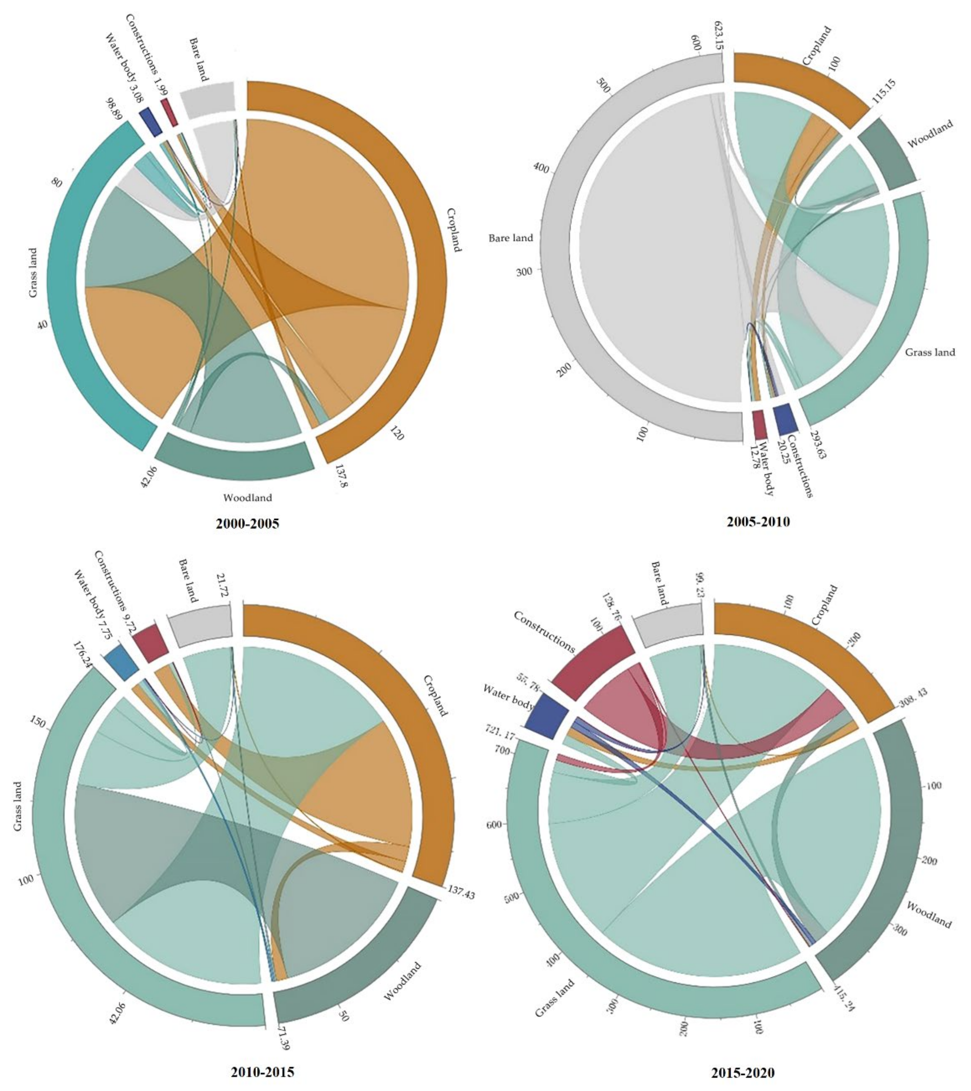
To fully understand the structural characteristics of land-use changes in the Hung River Valley during this period, a land-use transfer matrix was constructed to calculate the number of mutual land-use transfers from 2000 to 2020 (

Table 3. Land-use transfer matrix for the Hung River Valley (km²).

Years	Type	Cultivated Land	Forestland	Grassland	Water Areas	Construction	Bare Land
2000–2005	Cultivated land	—	4.29	49.7	0.9	0.96	0.25
	Forestland	3.44	—	33.78	0.37	0.1	0.63
	Grassland	88.55	35.57	—	1.49	0.8	13.32
	Water areas	8.91	1.04	4.85	—	0.1	0.15
	Construction	33.93	0.48	2	0.09	—	0.01
	Bare land	2.97	0.68	8.56	0.23	0.03	—
2005–2010	Cultivated land	—	10.52	135.32	3.61	7.5	2.26
	Forestland	6.61	—	63.14	0.85	0.21	5.6
	Grassland	105.6	61.06	—	2.55	4.56	604.67
	Water areas	13.08	2.14	6.19	—	0.51	10.38
	Construction	29.51	0.52	5.75	4.22	—	0.24
	Bare land	0.35	1.54	80.23	9.02		—
2010–2015	Cultivated land	—	4.87	70.84	3.63	7	0.36
	Forestland	6.52	—	62.74	1.06	0.21	0.69
	Grassland	70.02	64.34	—	2.45	1.83	20.45
	Water areas	4.41	0.85	6.07	—	0.23	0.22
	Construction	56.04	0.46	12.62	0.2	—	0
	Bare land	0.44	0.87	23.97	0.23	0	—
2015–2020	Cultivated land	—	26.22	219.07	15.84	104.28	1.43
	Forestland	25.19	—	376.38	11.26	1.89	4.88
	Grassland	218.72	374.21	—	17.65	21.28	91.87
	Water areas	16.17	7.09	21.97	—	1.26	1
	Construction	46.66	1.49	11.83	0.91	—	0.05
	Bare land	1.69	6.23	91.92	10.12	0.05	—

). As shown in the table, from 2000 to 2005, land-use shifts mainly occurred between arable land, grassland, and forest land, with a larger amount of arable land shifting to grassland and construction land. During the period 2010–2015, the trend of the previous period continued, with arable land always being the source of inflow of construction land and grassland, while the inflow and outflow of grassland and forest land were basically the same. From 2015 to 2020, the interconversion of various land uses made the inflow and outflow basically the same.

The land-use changes in the Hung River Valley in the past 20 years are mainly influenced by policies and urban expansion. In ecological protection policies, agricultural and livestock production and urbanisation, industrialisation, and other factors under the comprehensive effect of the Hung River Valley grassland, arable land, and construction land change dramatically. Each landscape flows between each other. Since 2002, Qinghai Province has fully implemented the policy of returning farmland to forest and grass, coupled with the establishment of many nature reserves. Arable land is in a net outflow situation, manifested in the expansion of grassland scale. At the same time, the Hung River Valley is an important axis of economic development in Qinghai Province, with intense human activity, high levels of urbanisation and industrialisation, and a continuous increase in the demand for construction land, the main source of which is the occupation of arable land.

3.2. Analysis of the Evolution of the Landscape Pattern Features

Since the magnitudes of different indicators are different, to facilitate comparison, the sampling of Z is standardized, as are all landscape pattern index values. As can be seen in Figure 3, NP and PD showed an increasing trend between 2000 and 2005, which is related to the partial conversion of arable land in the study area into forest land and grassland, and a large amount of arable land outflow, causing arable land fragmentation. After 2005, PD and NP gradually decreased, combined with the actual situation of the Hung River Valley. It can be seen that urban construction land encroachment on arable land, where there are many construction enclaves, merged with the original construction land, the main reason for the decline in PD and NP, in addition to the demolition and merging of rural settlements. LPI and AREA_MN increased slightly between 2000 and 2005 and fluctuated little after 2005, while DIVISION decreased slightly, indicating that the overall landscape pattern of the Hung River Valley showed a clustering trend after 2005.

The ED and LSI decreased slightly from 2000 to 2020, indicating that the overall landscape shape of the study area tends to be clustered, with the shape changing from complex to simple. conTAG increased relatively over the 20-year period, indicating that the overall landscape connectivity in the study area has increased. The Shannon Diversity Index (SHDI) decreased, and landscape heterogeneity diminished; the Shannon Evenness Index (SHEI) shows a decreasing trend, and the landscape type dominant over the overall landscape in the study area increased.

Changes in habitat quality are an indirect reflection of changes in different land types. To reveal in more detail the relationship between landscape changes in the study area and their impact on habitat quality, the characteristics of changes in different land types between 2000 and 2020 were calculated using Fragstats 4.2 (Figure 4). Grassland and woodland are important landscapes regarding the quality of habitat, with a decrease in the number of patches (NP), a decrease in density (PD), an increase in the mean patch area (AREA_MN), and a decrease in ED, LSI, and DIVISION from 2005–2020, indicating an overall clustering of landscape patterns and an increase in disturbance resistance in grassland. It is particularly important to note that the patches of built-up land in the study area decreased, and density decreased over the 20-year period, but ED increased slightly, and LSI and DIVISION remained largely unchanged, indicating that the landscape pattern in some areas became dispersed, which may be related to the extensive expansion of towns in Xining.

3.3. Spatial and Temporal Variation of Habitat Quality

The Habitat Quality Index (HQI) reflects the fragmentation of habitat patches in the study area, on the one hand, and the ability of habitat patches to resist the threat of habitat degradation brought about by human activities. On the other hand, its value is a continuous value between 0 and 1: the closer to 1, the better the habitat quality, indicating that biodiversity is better maintained. The raster areas of different classes and their percentages were counted (

Table 4. Habitat quality percentage statistics for the Huangshan Valley, 2000–2020.

Level	2000		2005		2010		2015		2020
	Area/km2	Percentage/%	Area/km2	Percentage/%	Area/km2	Percentage/%	Area/km2	Percentage/%	Area/km2	Percentage/%
Very low	2939.82	8.3	2972.32	8.4	2458.76	6.9	2554.65	7.3	2485.86	7.0
Low	3803.14	10.8	3760.62	10.7	3760.60	10.7	3714.35	10.5	3738.7	10.6
Medium	5726.48	16.3	5754.36	16.3	6633.74	18.8	6595.7	18.7	6632.13	18.8
High	16,038.43	45.5	16,012.46	45.4	15,606.80	44.3	15,583.67	44.2	15,573	44.0
Very high	6727.01	19	6735.09	19	6773.13	19.2	6786.52	19.3	6788.54	19.3

). To more accurately portray the evolution of habitat quality, using the Re-classify tool of the ArcGIS 10.6 software platform, habitat quality was classified into five levels: very low (0–0.2), low (0.2–0.4), medium (0.4–0.6), high (0.6–0.8), and very high (0.8–1), based on the actual situation in the Hung River Valley and with reference to existing studies [13,18].

From 2000 to 2020, the overall habitat quality showed an upward trend, and the global average habitat indexes were 0.656, 0.657, 0.661, 0.661, and 0.662, respectively. The main reason for this is that around 2000, Qinghai Province, based on its development orientation, successively carried out a series of ecological protection and restoration work, e.g., returning farmland to forest, returning farmland to grassland, and constructing nature reserves, which promoted the transformation of some medium- and high-grade habitat patches to higher-grade habitat patches.

On a spatial scale (Figure 5), the quality of habitats in the concentrated areas of woodland, grassland, and watersheds is high, while the quality of habitats on arable land, construction land, and bare land is low. The whole area is dominated by habitat patches of excellent grade. Habitat quality in the north, east, and west districts of Xining is low compared to other areas, due to the deteriorating ecological conditions in the central areas of Xining as a result of increasingly intense human activities. Among all areas, the habitat quality indexes of Datong County, Guide County, Mutual Aid County, Menyuan County, and Zunhua County all exceed 0.7, with Guide County being the highest, maintaining a level of 0.9; Hualong County, Jianzha County, Ping’an County, and Minhe County all show an increasing trend, with Hualong County being the highest and Minhe County being relatively low; the socio-economic development of Huangyuan County and Huanzhong County is strongly affected by the radiation of Xining City, and the social and economic development has a greater impact on the ecological environment.

3.4. Hotspot Analysis of the Spatial Distribution of Habitat Quality

3.4.1. Overall Clustering Characteristics

To explore the spatial differentiation characteristics of habitat quality in the Hung River Valley in more detail, the study area was divided into 2328 4 × 4 km grids using grid analysis. The mean values of habitat quality in 2000, 2005, 2010, 2015, and 2020 were extracted from 18 counties and cities in the Hung River Valley based on grid scale, and the ArcGIS 10.6 platform was used to calculate the spatial clustering of habitat quality in the study area from 2000 to 2020.

The Moran’s I calculations for the five periods of 2000, 2005, 2010, 2015, and 2020 showed that the Z scores of the five periods were all above 75 and much higher than 2.58, and the p-values passed the 1% significance test, indicating that the spatial distribution of habitat quality values in the Hung River Valley was not random at a 99.9% confidence level and that there was significant spatial correlation (

Table 5. Global Moran’s I Index table.

Year	Global Autocorrelation Index Statistics			Result
	Moran’s I	Z-Score	p-Value
2000	0.699	46.929	0.0000	Gather
2005	0.698	46.886	0.0000	Gather
2010	0.705	47.344	0.0000	Gather
2015	0.777	51.755	0.0000	Gather
2020	0.706	47.427	0.0000	Gather

).

The Moran’s I index for all five periods was greater than 0.65, showing a significant pattern of aggregation, i.e., high values of habitat quality clustered in space, and low values tended to be adjacent to each other. Since 2000, the aggregation effect of habitat quality in the Hung River Valley has been increasing on the whole; however, from 2015 to 2020, the aggregation effect has been on the decline, mainly because the areas with high habitat quality are affected by the expansion of urban land, eroding the original woodland, grassland, and other ecological landscapes and causing habitat fragmentation. The development of a large amount of urban land has led to an increasingly widespread distribution of areas with a low habitat quality. This is shown in Table 5.

3.4.2. Local Agglomeration Characteristics

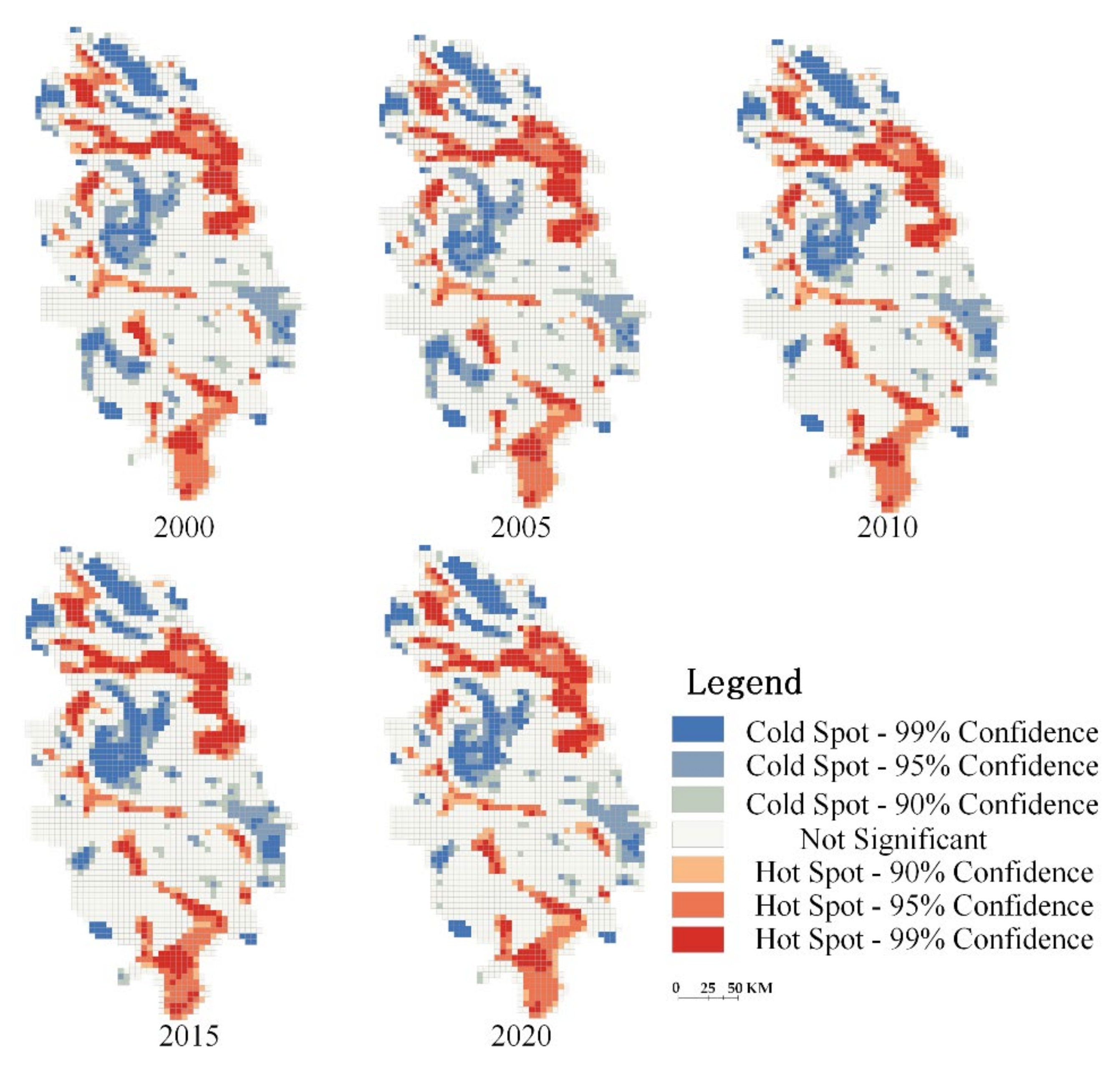
The global spatial autocorrelation can only reflect whether there are agglomerative features in the study area as a whole and cannot clarify the location distribution of agglomerative features. Based on the ArcGIS 10.6 platform, a hotspot analysis was conducted based on a grid, and cold spots and hotspots with a confidence level above 90% were selected to reflect the distribution of high- and low-value habitat quality clusters in the Hung River Valley (Figure 6).

During 2000–2020, the Hung River Valley habitat quality changes show obvious regional differences “Guide-Ledu”, south of the line of the habitat quality index, including Ping’an County, Ledu District, Tongren County, and Guide County, generally improved. This is mainly due to the implementation of ecological protection policies, e.g., returning farmland to forest and grass, and establishing establishment many nature reserves, scenic spots, forest parks, and geoparks, such as the Mengda Nature Reserve and the Sanjiangyuan Nature Reserve. The overall habitat quality north of the “Guide-Ledu” linkage has a significant spatial aggregation effect, but the change effect is not obvious, and there are cold spots in Xining City and surrounding counties. The cold spot area is concentrated in Xining City, which is the political and economic centre of Qinghai Province and the gathering area of arable land, and the intense production and construction and agricultural activities have interfered with the ecological environment, resulting in the clustering and distribution of low habitats in the area. Mutual Aid County and Ping’an County are adjacent to Xining. Mutual Aid County has the largest population and the most intense human activities in Haidong, thus showing a secondary cold point concentration distribution, and the habitat cold point rose and then declined between 2000 and 2020, dropping to the lowest point in 2015 with the worst habitat quality.

3.5. Spatial Response of Habitat Quality to Urbanisation

The spatial pattern of habitat reflects that human activities and natural elements are important influencing factors of spatial differentiation of habitat quality. Among these factors, human activity status has gradually become the main independent variable of habitat quality. Natural factors, such as slope, average annual rainfall, average annual temperature, and elevation, and urbanisation process elements such as population density, gross domestic product, and the night light index, are selected as independent variables. The optimal model was selected by a comparative analysis of GWR and ordinary least squares (OLS). The coefficient of variance expansion is a measure of the severity of multiple (multiple) collinearities in a multiple linear regression model. It represents the ratio of the variance of the regression coefficient estimator to the variance, assuming that the independent variables are not linearly correlated. Usually, 10 is used as the judgment boundary. When VIF < 10, there is no multicollinearity; when 10 ≤ VIF < 100, there is strong multicollinearity; when VIF ≥ 100, there is severe multicollinearity.

The results show that the VIF of the natural and socio-economic factors in the OLS model is less than 10, and there is no covariance between the variables, which satisfies the requirements of the explanatory variables. The explanatory power of the OLS model for habitat quality was less than 50%, and the goodness of fit of the GWR model was significantly higher than that of the OLS model in all five time sections, with its explanatory power reaching more than 90%. Meanwhile, the Sigma and AICc in the GWR model were lower than those of the OLS model, indicating that the GWR model had better explanatory power for the factors influencing habitat quality and its model accuracy was better (

Table 6. GWR model goodness of fit.

Model Parameters	2000	2005	2010	2015	2020
Bandwidth	55	55	55	55	55
Residual Squares	230.377	238.716	233.701	228.572	228.182
Effective Number	536.451	534.240	532.123	529.740	529.882
Sigma	0.353	0.359	0.355	0.351	0.351
AICC	6338.648	2661.698	2604.091	2543.320	2539.722
R2	0.903	0.900	0.902	0.904	0.904
Adjusted R2	0.875	0.871	0.874	0.877	0.877

and

Table 7. GWR global regression coefficients.

Global Regression Coefficients	2000	2005	2010	2015	2020
DEM (Digital elevation model)	0.119	0.127	0.247	0.236	0.246
SLOPE	0.324	0.352	0.344	0.343	0.342
RAIN	0.187	0.190	0.175	0.171	0.175
TEM	0.217	0.234	0.348	0.339	0.349
GDP	−0.067	−0.012	0.036	0.017	0.036
LIGHT	−0.030	−0.089	−0.177	−0.187	−0.176
POP	−0.049	−0.060	−0.031	−0.015	−0.021

).

Slope and elevation are important natural factors influencing habitat quality. However, due to the interaction of human activities, the correlation between habitat quality and natural factors such as slope and elevation is complicated. As can be seen in Figure 7, slope, elevation, and habitat quality generally show a positive relationship, with the positive and negative effects of slope on habitat being relatively complexly distributed within a geographical area. The positive correlation between slope and habitat is mainly concentrated in mountainous and hilly areas and areas with continuous construction land, and the positive correlation between height and slope is distributed in discontinuous bands. The central region is flat. Human activities are relatively frequent, and the natural ecological space is encroached upon by construction land, resulting in serious habitat degradation. Some of the hilly areas are affected by human development and construction activities, and the habitats are damaged to a certain extent, while the green areas and water areas in the plains are better protected by ecological protection, and the overall level of habitats is higher; under the influence of human activities, the slope of the area is negatively correlated with habitat quality. The areas with a high positive correlation between elevation and habitat quality are mainly concentrated in the hilly areas, with a cluster and circle pattern of distribution. In general, natural factors such as slope and elevation play an important role in the overall pattern of habitat distribution. With higher slope and elevation, socio-economic activities are generally less frequent in the area, and the disturbance factors to the ecosystem are smaller, so the impact on habitat quality is relatively small. In plain areas, where human activities are frequent, socio-economic factors have a more prominent impact on habitat quality than do natural factors.

Urbanisation factors such as population density, gross domestic product, and the night-time light index have a more significant negative correlation with habitat quality (Figure 6). The negative correlation between population density and habitat quality is most significant and widely distributed: During the study period, the negative influence of the northern and central zones was further expanded, because the central zone was influenced by the economic radiation of Xining, and the towns were developed significantly, with a relatively obvious population growth, which increased the pressure on the ecological carrying capacity of the surrounding areas. The high density of economic activities also contributed to the fragmentation of the landscape pattern and the encroachment of arable land and construction land on ecological land.

The regression coefficients of the economic impact on habitat show that the negative impact in the study area is less intense. The reason for this is that the study area is affected by the policy of “returning farmland to forest” and “returning farmland to grass” in Qinghai Province, and the GDP output value of mainly arable land is low, so the negative impact on habitat is weak. The northern and southern parts of the city have seen rapid economic development, and the ecological environment has been significantly disturbed by economic activities. The night-time light index characterises the indirect disturbance effect of urban socio-economic development and high intensity human activities on the ecosystem: In 2000, the positively correlated areas were mainly scattered in clusters in the plains, while the negatively correlated areas were widely distributed, with the most intense negative impact in the mountainous hills. Between 2000 and 2010, the areas with intense negative correlation and the positively correlated areas both decreased. However, the negative correlation dominated the region, and the trend from the mountains to the plains was stronger and weaker. Between 2010 and 2020, the areas with strong negative correlations expanded again, which was related more to urban development. Overall, the agglomeration of factors in the urbanisation process is an important driver of regional habitat quality change, and the spatial heterogeneity of the impact of socio-economic factors on habitat quality is more significant as the rate of urbanisation accelerates.

4. Discussion

4.1. Scaling Effects of Land Characteristics and Habitat Quality

The coupling of landscape patterns and ecological processes reflected in land use is a central theme in landscape ecology research [35,36,37]. The resolution of the spatial characteristics of land-use has long been the focus and difficulty of scholars studying landscape ecology [38,39,40]. Because the relationship between patterns and processes is often non-linear and shows multi-factor interaction and time-lagged effects [41]. Differences in scale and accuracy can cause the type, number, and spatial distribution characteristics and configurations of land-use units to reflect different patterns and process couplings [42,43,44].

The use of the InVEST model to evaluate spatial and temporal changes in regional habitat quality is mainly based on land-use data for model input. In the process of revealing the drivers of habitat quality change, the drivers of the same evaluation unit will reflect different intensities of influence on different scales of habitat quality units [41,42]. For human activities, the study of land-use change processes and their ecological effects is also a process impact on patterns, but such impacts often involve time scales of years or decades, so the impact of “fast” ecological processes on landscape patterns has a lag in time scale [44]. This and numerous studies have expressed the mismatch in time scales between landscape patterns and ecological processes, leading to a certain lack of understanding of feedback mechanisms and systems as a whole [44,45,46,47].

Therefore, research on the effects of land characteristics and habitat quality scales needs to be further investigated, with a focus on the integration of natural, socio-economic, and human factors to resolve the complexity of the landscape in breadth and on the coupling of macroscopic patterns and microscopic processes [44,48]. Providing a reliable basis for macro-pattern characterisation and management strategy formulation, along with macro-pattern planning and management, will in turn strengthen the practical significance of micro-research [49]. The ultimate goal is to scientifically, rationally, and accurately reveal the important influencing factors of habitat quality change due to land-use change [50,51].

4.2. Research Shortcomings

The InVEST model is relatively mature and outperforms traditional methods in terms of spatial expression and dynamic research, but there is a certain degree of subjectivity in the parameter settings in the calculations, and the validation of the parameters and the assessment of their rationality are worth exploring in depth [10,24,26]. This study explores the effects of factor agglomeration on habitat in the urbanisation process and obtains some insights that are beneficial to ensuring ecological safety in the urbanisation process. As a complex social-ecological system, the impact of urbanisation on habitat quality includes not only economic and demographic factors, but also hidden factors such as culture and policies [42,43], and there is a complex relationship between factors in the urbanisation process, so it is necessary to introduce more social factors and clarify the interrelationships between them for a comprehensive study. This is a direction for further research.

4.3. Policy Recommendations

The Hung River Valley is a concentrated area of arable land in Qinghai Province, which requires the continuous optimisation of agricultural production methods and improvement of agricultural production efficiency. At the same time, in the context of the work on comprehensive land improvement and ecological protection and restoration, the region’s landscape type characteristics and current ecological problems should be combined to promote agricultural production and ecological protection and restoration in an integrated manner using development, preparation, reclamation, and restoration. Compared to areas such as Datong and GuiDe counties, there is more room to improve the quality of habitats in the cities of Xining and Haidong, and there is a need to further promote the construction of large-scale forest farms and accelerate the implementation of ecological construction projects such as the greening of key areas in central cities, major towns and parks, and urban wetland parks, in order to systematically improve the quality of regional habitats. A fragmented and complex landscape distribution is not conducive to the protection and restoration of ecosystems; thus, when formulating and implementing relevant measures, it is necessary to adhere to the principle of integrated management of “mountains, water, forests, fields, lakes, and grasses”, reduce the risk of excessive intervention caused by the management of single elements, and maintain natural and semi-natural landscapes.

5. Conclusions

(1)

From 2000 to 2020, the area of grassland, construction land, and watersheds in the Hung River Valley increased year by year. The area of cropland kept decreasing. The woodland and bareland fluctuated and changed, but was basically stable. Among them, the main source of growth in construction land is the occupation of cropland, which is especially obvious in Xining and Haidong; woodland, grassland, water, and other high habitat landscape types increased steadily, thanks to the implementation of policies returning farmland to forest and grass and establishing nature reserves at all levels.

(2)

From 2000 to 2020, the Hung River Valley Habitat Quality Index was stable, at around 0.66, with a slight increase. The regional habitat quality changed, and hot and cold states on both sides of the “Guide-Ledu” were differently distributed. The habitat level of Xining showed low-quality characteristics, including decreasing and gathering cold spots, while the habitat quality index of Datong County, Guide County, Mutual County, Menyuan County, and Zunhua County was higher. The ecological protection pressure is relatively small.

(3)

The natural elements shaped the overall habitat distribution pattern in the Hung River Valley, with slope, elevation, and habitat quality generally showing a positive relationship, and the effect of slope on habitat was relatively complex. The effects of disturbance on the ecosystem were strong, biodiversity was destroyed, ecosystem imbalance occurred, and habitat quality was significantly degraded.

References

1. Costanza, R.; D’Arge, R.; De Groot, R.; Farber, S.; Grasso, M.; Hannon, B.; Limburg, K.; Naeem, S.; O’Neill, R.V.; Paruelo, J.; et al. The value of the world’s ecosystem services and natural capital. Nature 1997, 387, 253–260. [Google Scholar] [CrossRef]
2. Ellis, E.C.; Pascual, U.; Mertz, O. Ecosystem services and nature’s contribution to people: Negotiating diverse values and trade-offs in land systems. Curr. Opin. Environ. Sustain. 2019, 38, 86–94. [Google Scholar] [CrossRef]
3. Fellman, J.B.; Hood, E.; Dryer, W.; Pyare, S. Stream physical characteristics impact habitat quality for pacific salmon in two temperate coastal watersheds. PLoS ONE 2015, 10, e0132652. [Google Scholar] [CrossRef] [Green Version]
4. Gao, Y.; Ma, L.; Liu, J.; Zhuang, Z.; Huang, Q.; Li, M. Constructing ecological networks based on habitat quality assessment: A case study of Chang-zhou, China. Sci. Rep. 2017, 7, 46073. [Google Scholar] [CrossRef] [PubMed]
5. Sharp, R.; Tallis, H.T.; Ricketts, T.; Guerry, D.A.; Wood, A.S.; Chaplin-Kramer, R.; Nelson, E.; Ennaanay, D.; Wolny, S.; Olwero, N.; et al. InVEST 3.2.0 User’s Guide; The Natural Capital Project; Stanford University, University of Minnesota, The Nature Conservancy, World Wildlife Fund: Minneapolis, MN, USA, 2018. [Google Scholar]
6. Hillard, E.M.; Nielsen, C.K.; Groninger, J.W. Swamp rabbits as indicators of wildlife habitat quality in bottomland hardwood forest ecosystems. Ecol. Indic. 2017, 79, 47–53. [Google Scholar] [CrossRef]
7. Peng, J.; Pan, Y.; Liu, Y.; Zhao, H.; Wang, Y. Linking ecological degradation risk to identify ecological security patterns in a rapidly urbanizing landscape. Habitat Int. 2018, 71, 110–124. [Google Scholar] [CrossRef]
8. Barbara, R.; Stefan, L. A spatially explicit patch model of habitat quality, integrating spatio-structural indicators. Ecol. Indic. 2018, 94, 8–14. [Google Scholar]
9. Janus, J.; Bozek, P. Land abandonment in Poland after the collapse of socialism: Over a quarter of a century of increasing tree cover on agricultural land. Ecol. Eng. 2019, 138, 106–117. [Google Scholar] [CrossRef]
10. Liu, Y.; Huang, X.; Yang, H.; Zhong, T. Environmental effects of land use/cover change caused by urbanization and policies in South-west China Karstarea: A case study of Guiyang. Habitat Int. 2014, 44, 339–348. [Google Scholar] [CrossRef]
11. Terrado, M.; Sabater, S.; Chaplin-Kramer, B.; Mandle, L.; Ziv, G.; Acuña, V. Model development for the assessment of terrestrial and aquatic habitat quality in conservation planning. Sci. Total Environ. 2016, 540, 63–70. [Google Scholar] [CrossRef] [Green Version]
12. Sala, O.E.; Chapin, F.S.; Armesto, J.J.; Berlow, E.L.; Bloomfield, J.; Dirzo, R.; Hubersanwald, E.; Huenneke, L.F.; Jackson, R.B.; Kinzig, A.P.J.S. Global biodiversity scenarios for the year 2100. Science 2000, 287, 1770–1774. [Google Scholar] [CrossRef] [PubMed]
13. Liu, C.H.; Lun, Y. Progress, achievements and prospects of biodiversity protection in Yunnan Province. Biodivers. Sci. 2020, 29, 200. [Google Scholar] [CrossRef]
14. Liu, Y.; Zhou, Y.; Du, Y. Study on the Spatio-Temporal Patterns of Habitat Quality and Its Terrain Gradient Effects of the Middle of the Yangtze River Economic Belt Based on InVEST Model. Resour. Environ. Yangtze Basin. 2019, 28, 2429–2440. [Google Scholar]
15. Lei, J.C.; Liu, J.X.; Yong, F.; Liu, H.M.; Wu, J.; Ding, H.; Wang, J.M.; Wu, S.Q.; Cheng, S.; Cui, P. Multi- Scenario Ecosystem Service Assessment of Wuma River Valley Based on CLUE- S and InVEST Models. J. Ecol. Rural Environ. 2017, 33, 1084–1093. [Google Scholar]
16. Liang, X.; Liu, X.P.; Li, X.; Chen, Y.M.; Tian, H.; Yao, Y. Delineating multi-scenario urban growth boundaries with a CA-based FLUS model and morphological method. Landsc. Urban Plan. 2018, 177, 47–63. [Google Scholar] [CrossRef]
17. Koull, N.; Chehma, A. Soil characteristics and plant distribution in saline wetlands of Oued Righ, northeastern Algeria. J. Arid. Land. 2016, 8, 948–959. [Google Scholar] [CrossRef]
18. Wei, H.; Zhao, W.W.; Zhang, X.; Wang, X.Z. Regional ecosystem service value evaluation based on land use changes: A case study in Dezhou, Shandong Province, China. Acta Ecol. Sin. 2017, 37, 3830–3839. [Google Scholar]
19. Kim, T.; Song, C.; Lee, W.K.; Kim, M.; Lim, C.H.; Jeon, S.W.; Kim, J. Habitat quality valuation using InVEST model in Jeju Island. J. Korea Soc. Environ. Restor. Technol. 2015, 18, 1–11. [Google Scholar] [CrossRef] [Green Version]
20. Qamer, F.M.; Shehzad, K.; Abbas, S.; Murthy, M.; Xi, C.; Gilani, H.; Bajracharya, B. Mapping Deforestation and Forest Degradation Patterns in Western Himalaya, Pakistan. Remote Sens. 2016, 8, 385. [Google Scholar] [CrossRef] [Green Version]
21. Shalaby, A.; Tateishi, R. Remote sensing and GIS for mapping and monitoring land cover and land-use changes in the Northwestern coastal zone of Egypt. Appl. Geogr. 2007, 27, 28–41. [Google Scholar] [CrossRef]
22. Zhang, H.Y.; Wang, L.; Zhao, R.; Liang, Y. Integrating landscape pattern with economic indices to conduct land use two-dimensional division: Taking Qinghai Province as an example. Bull. Surv. Mapp. 2013, 3, 82–85. [Google Scholar]
23. Zhao, D.Y.; Zeng, Y.N. Land use changes and ecological risk assessment in eastern Qinghai Plateau: A case study in Haidong, Qinghai, China. J. Desert Res. 2016, 36, 1190–1197. [Google Scholar]
24. Wu, B.W.; Yang, S.T.; Shao, N.F.; Peng, R.W.; Guan, Y.B. Effects of land use change on ecosystem service value in fragile ecological area of the Loess Plateau: A case study of Fenhe River Basin. Res. Soil Water Conserv. 2019, 26, 340–345. [Google Scholar]
25. Hou, L.W. InVEST habitat quality model parameter assignment discussion. Environ. Dev. 2017, 29, 80–81. [Google Scholar]
26. Newbold, T.; Hudson, L.N.; Hill, S.L.L.; Contu, S.; Lysenko, I.; Senior, R.A.; Börger, L.; Bennett, D.J.; Choimes, A.; Collen, B.; et al. Global effects of land use on local terrestrial biodiversity. Nature 2015, 520, 45–50. [Google Scholar] [CrossRef] [PubMed] [Green Version]
27. Hennig, E.I.; Schwick, C.; Soukup, T.; Orlitová, E.; Kienast, F.; Jaeger, J.A.G. Multi-scale analysis of urban sprawl in Europe: Towards a European de-sprawling strategy. Land Use Policy 2015, 49, 483–498. [Google Scholar] [CrossRef] [Green Version]
28. Xinliang, X.; Jiyuan, L.; Shuwen, Z.; Rendong, L.; Changzhen, Y.; Shixin, W. China Multi-Period Land Use and Land Cover Remote Sensing Monitoring Dataset (CNLUCC); Data Registration and Publishing System of the Resource and Environmental Science Data Center of the Chinese: Shanghai, China, 2020. [Google Scholar] [CrossRef]
29. McDonald, R.I.; Weber, K.; Padowski, J.; Flörke, M.; Schneider, C.; Green, P.A.; Gleeson, T.; Eckman, S.; Lehner, B.; Balk, D.; et al. Water on an urban planet: Urbanization and the reach of urban water infrastructure. Glob. Environ. Chang. 2014, 27, 96–105. [Google Scholar] [CrossRef] [Green Version]
30. Deng, Y.J.; Yao, S.B.; Hou, M.Y.; Zhang, T.Y.; Lu, Y.N.; Gong, Z.W.; Wang, Y.F. Assessing the effects of the Green for Grain Program on ecosystem carbon storage service by linking the InVEST and FLUS models: A case study of Zichang county in hilly and gully region of Loess Plateau. J. Nat. Resour. Energy 2020, 35, 826–844. [Google Scholar]
31. Wu, Y.Z.; Shan, L.P.; Guo, Z.; Peng, Y. Cultivated land protection policies in China facing 2030: Dynamic balance system versus basic farmland zoning. Habitat Int. 2017, 69, 126–138. [Google Scholar] [CrossRef]
32. Wang, C.D.; Li, X.; Yu, H.J.; Wang, Y.T. Tracing the spatial variation and value change of ecosystem services in Yellow River Delta, China. Ecol. Indic. 2019, 96, 270–277. [Google Scholar] [CrossRef]
33. Shi, H.; Li, X.; Yang, Z.Z.; Li, T.H.; Ren, Y.; Liu, T.T.; Yang, N.D.; Zhang, H.; Chen, G.Z.; Liang, X. Tourism land use simulation for regional tourism planning using POIs and cellular automata. Trans. GIS 2020, 24, 1119–1138. [Google Scholar] [CrossRef]
34. Sharma, R.; Nehren, U.; Rahman, S.A.; Meyer, M.; Rimal, B.; Seta, G.A.; Baral, H. Modeling Land Use and Land Cover Changesn and Their Effects on Biodiversity in Central Kalimantan, Indonesia. Land 2018, 7, 57. [Google Scholar] [CrossRef] [Green Version]
35. Gustafson E, J. Quantifying landscape spatial pattern: What is the state of the art? Ecosystems 1998, 1, 143–156. [Google Scholar] [CrossRef]
36. Van der Biest, K.; Meire, P.; Schellekens, T.; D’hondt, B.; Bonte, D.; Vanagt, T.; Ysebaert, T. Aligning biodiversity conservation and ecosystem services in spatial planning: Focus on ecosystem processes. Sci. Total Environ. 2020, 712, 136350. [Google Scholar] [CrossRef] [PubMed]
37. Lin, W.B.; Sun, Y.M.; Nijhuis, S.; Wang, Z.L. Scenario-based flood risk assessment for urbanizing deltas using future land-use simulation (FLUS): Guangzhou Metropolitan Area as a case study. Sci. Total Environ. 2020, 739, 139899. [Google Scholar] [CrossRef]
38. Liu, X.J.; Li, X.; Liang, X.; Shi, H.; Ou, J.P. Simulating the Change of Terrestrial Carbon Storage in China Based on the FLUS-InVEST Model. Trop. Geogr. 2019, 39, 397–409. [Google Scholar]
39. Di Febbraro, M.; Sallustio, L.; Vizzarri, M.; De Rosa, D.; De Lisio, L.; Loy, A.; Eichelberger, B.; Marchetti, M. Expert-based and correlative models to map habitat quality: Which gives better support to conservation planning? Glob. Ecol. Conserv. 2018, 16, e00513. [Google Scholar] [CrossRef]
40. Zhu, J.; Ding, N.; Li, D.; Sun, W.; Xie, Y.; Wang, X. Spatiotemporal Analysis of the Nonlinear Negative Relationship between Urbanization and Habitat Quality in Metropolitan Areas. Sustainability 2020, 12, 669. [Google Scholar] [CrossRef] [Green Version]
41. Sun, L.; Yang, L.; Chen, L.D.; Zhao, F.K.; Li, S.J. Hydraulic redistribution and its contribution to water retention during short-term drought in the summer rainy season in a humid area. J. Hydrol. 2018, 566, 377–385. [Google Scholar] [CrossRef]
42. Priyadarshini, K.V.R.; Prins, H.H.T.; De Bie, S.; Heitknig, I.M.A.; Woodborne, S.; Gort, G.; Kirkman, K.; Ludwig, F.; Dawson, T.E.; De Kroon, H. Seasonality of hydraulic redistribution by trees to grasses and changes in their water-source use that change tree-grass interactions. Ecohydrology 2016, 9, 218–228. [Google Scholar] [CrossRef]
43. Tang, Z.; Ma, J.; Peng, H.; Wang, S.; Wei, J. Spatiotemporal changes of vegetation and their responses to temperature and precipitation in upper Shiyang river basin. Adv. Space Res. 2017, 60, 969–979. [Google Scholar] [CrossRef]
44. Hu, Y.N.; Mei, L.; Wei, J.G. Spatial differentiation and dynamic mechanism of regional travel agency efficiency in China based on GWR model. Sci. Geogr. Sin. 2018, 38, 107–113. [Google Scholar]
45. Zhai, T.; Wang, J.; Fang, Y.; Qin, Y.; Huang, L.; Chen, Y. Assessing ecological risks caused by human activities in rapid urbanization coastal areas: Towards an integrated approach to determining key areas of terrestrial-oceanic ecosystems preservation and restoration. Sci. Total Environ. 2020, 708, 135153. [Google Scholar] [CrossRef] [PubMed]
46. Li, F.; Wang, L.; Chen, Z.; Clarke, K.C.; Li, M.; Jiang, P. Extending the SLEUTH model to integrate habitat quality into urban growth simulation. J. Environ. Manag. 2018, 217, 486–498. [Google Scholar] [CrossRef] [Green Version]
47. Gu, X.; Long, A.; Liu, G.; Yu, J.; Wang, H.; Yang, Y.; Zhang, P. Changes in Ecosystem Service Value in the 1 km Lakeshore Zone of Poyang Lake from 1980 to 2020. Land 2021, 10, 951. [Google Scholar] [CrossRef]
48. Nematollahi, S.; Fakheran, S.; Kienast, F.; Jafari, A. Application of InVEST habitat quality module in spatially vulnerability assessment of natural habitats (case study: Chaharmahal and Bakhtiari province, Iran). Environ. Monit. Assess. 2020, 192, 1–17. [Google Scholar] [CrossRef] [PubMed]
49. Anchang, J.Y.; Ananga, E.O.; Pu, R. An efficient unsupervised index based approach for mapping urban vegetation from IKONOS imagery. Int. J. Appl. Earth Obs. Geoinform. 2016, 50, 211–220. [Google Scholar] [CrossRef]
50. Gong, P.; Li, X.; Wang, J.; Bai, Y.; Chen, B.; Hu, T.; Liu, X.; Xu, B.; Yang, J.; Zhang, W.; et al. Annual maps of global artificial impervious area (GAIA) between 1985 and 2018. Remote Sens. Environ. 2020, 236, 111510. [Google Scholar] [CrossRef]
51. Ma, Y.; Zhang, S.; Yang, K.; Li, M. Influence of spatiotemporal pattern changes of impervious surface of urban megaregion on thermal environment: A case study of the Guangdong—Hong Kong—Macao Greater Bay Area of China. Ecol. Indic. 2021, 121, 107106. [Google Scholar] [CrossRef]
Figure 1. Location of the Hung River Valley area.
Land 10 01369 g001
Figure 2. Sankey Diagram of Land-Use Transfer.
Land 10 01369 g002
Figure 3. Hung River Valley overall landscape pattern trend evolution map, 2000–2020.
Land 10 01369 g003
Figure 4. Evolution of landscape pattern indices for different land types in the Hung River Valley, 2000–2020.
Land 10 01369 g004
Figure 5. Spatial Distribution of habitat quality in the Hung River Valley, 2000–2020.
Land 10 01369 g005
Figure 6. Habitat quality “hotspots” analysis in the Hung River Valley, 2000–2020.
Land 10 01369 g006
Figure 7. Spatial distribution patterns of GWR regression coefficients.
Land 10 01369 g007