
Strategies to Mitigate the Deteriorating Habitat Quality in Dong Trieu District, Vietnam


1
Department of Soil and Environmental Sciences, National Chung Hsing University, Taichung City 402, Taiwan
2
Department of Land Planning, Faculty of Natural Resources and Environment, Vietnam National University of Agriculture, Hanoi City 12406, Vietnam
3
Innovation and Development Center of Sustainable Agriculture, National Chung Hsing University, Taichung City 402, Taiwan
*
Author to whom correspondence should be addressed.
Land 2022, 11(2), 305; https://0-doi-org.brum.beds.ac.uk/10.3390/land11020305
Submission received: 15 January 2022
/
Revised: 11 February 2022
/
Accepted: 14 February 2022
/
Published: 17 February 2022
(This article belongs to the Section Land Socio-Economic and Political Issues)
Abstract
:Dong Trieu district is a vital connection for territorial ecological security and human welfare between Hanoi (the capital of Vietnam) and Quang Ninh province. Therefore, habitat quality (HQ) is of extraordinary importance to the area’s sustainable development. The ArcGIS platform, Dyna-CLUE, and InVEST models were utilized in this study to assess the spatial and temporal transformations of land use and the changes of HQ in 2030 under various scenarios, with intentions to find strategies that may mitigate the HQ’s deteriorating trend in the district. Simulated results indicated that, assuming the development is maintained as usual, the average HQ of the District at 2030 could diminish by 0.044 from that of 2019 (a four-times decrease compared to the previous decade). Cases comprised of four basic scenarios, including development as usual, built-up expansion slowdown, forest protection emphasized, and agricultural land conversion, were used to identify potential strategies to mitigate the deteriorating trend. Simulated results revealed that keeping the built-up expansion rate lower than 100 ha y−1, the deforestation rate lower than 20 ha y−1, and preferring orchards over agricultural land conversion is required to limit the drop in HQ to within 0.01 in the next decade. Other than the existing population growth control policy, new guidelines such as (1) changing urban expansion type from outward to upward to control the built-up expansion rate, (2) substituting forest-harming industries to forest-preservation industries to reduce deforestation rate, (3) encouraging orchards preferred over agricultural land conversion to increase incomes while maintaining higher habitat quality, (4) practicing better farming technologies to improve crop production and to alleviate potential food security issues due to considerable reduction in cropland, and (5) promoting Green Infrastructure and the Belt and Road Initiative to increase urban green cover and raise residents’ income should be considered in designing the new mitigation strategies.
1. Introduction
Habitat quality (HQ) indicates the ability of an ecosystem to support the distribution of species in space and the potential of resource acquisition [1]. A high-quality habitat supports richer biodiversity, while the decrease in HQ leads to a decline in biodiversity [2]. The HQ is influenced by natural and anthropogenic factors, including topography, landforms, vegetation cover, and human population density. It is well known that intensive anthropocentric activities, such as deforestation and urban expansion, can prompt a far and wide loss of species, habitat degradation, and fragmentation [3,4].
On evaluating the HQ of a region, earlier research was often based on monitoring the biodiversity changes within the study region [5,6,7]. However, biodiversity surveys are time-consuming and labor-intensive and are usually limited within a small area or specific nature reserves. In addition, field biodiversity surveys cannot maintain long-duration dynamic sequence monitoring because of their high cost. Recently, with the advancements in the global positioning system, geographic information system, and remote sensing technologies, numerous ecological models have been used to evaluate the HQ. For example, the environmental niche model was used for finding that organism’s role within that environment [8,9,10], the habitat suitability index models (HIS) have been utilized to assess preservation plans and the possible effects of management measures on HQ [11,12], but many species-specific data are required to run the niche and the HIS models. However, the Integrated Valuation of Environmental Services and Tradeoffs model (InVEST) does not require data about the species’ distribution or presence. It is thus a powerful tool that can monitor biodiversity and HQ dynamics, especially in areas with limited available data on biodiversity. For example, the InVEST model has been utilized to analyze temporal and spatial changes in HQ from the viewpoint of the Red-crowned crane (Grus japonensis) in the national nature reserve for rare birds of China [13] and assessing the land-use changes and their consequences on HQ of Henan’s water sources [14]. Wu et al. [15] combined remote sensing (RS) technology and the InVEST model to evaluate HQ’s temporal and characteristic changes to find its driving factors in Guangdong–Hong Kong–Macao greater bay area. Li et al. [16] investigated the evolution of HQ and the terrain gradient effect of HQ in northwest Hubei province from 2000 to 2020 based on land-use data and the digital elevation model (DEM). The InVEST and Markov models were combined in [17] to quantitatively evaluate the HQ and landscape pattern in the Hubei section of the Three Gorges reservoir area. Xu et al. [18] explored the effects of land-use and landscape patterns changes on HQ over two decades in the Taihu lake basin using RS data. Berta Aneseyee et al. [19] used the InVEST model and Pearson correlation to estimate the relationship of HQ with various underlying factors in the Omo-Gibe basin, southwest Ethiopia, quantitatively.
The abovementioned research generated HQ maps showing values of HQ ranging from 0 to 1, where 1 indicates the highest suitability for species. Different land-use/land cover (LULC) types have various sensitivities to threat sources. The sensitivity is determined mainly based on the fundamental theories of ecology and landscape ecology and the basic principles of biodiversity conservation. Average HQ index decrease in one decade often ranges from 0.0015 to 0.02 [13,14,15,16,17], while considerable decreases, by 0.04 to 0.06, have been observed in some river basins [18,19]. An HQ decrease by 0.01 is considered significant enough to threaten the species [13]. Furthermore, researchers found that the changes in LULC played a significant role in the HQ dynamics. They also indicated that the ecosystem service, landscape pattern, and forest fragmentation were highly sensitive to LULC change conditions [13,14,15,16,17,18,19]. The LULC maps generated from the satellite images are based on the availability of the satellite images [13,14,15,16,17], thus, they are limited to the historical and recent periods. However, the future LULC scenarios can be simulated with a land-use model. The land-use simulation models utilized must be able to address two independent issues: where land-use changes are probably going to occur (area of change) and at what speed those changes are probably going to progress (amount of changes) [20,21]. Based on their basic designs, the models can be separated into top-down and bottom-up models. The top-down models are generally utilized when it is possible to estimate the land-use change’s rate of whole areas through land-use statistics or mathematic equations [21]. On the other hand, the bottom-up models are used to demonstrate the effects of various land users, such as individuals, institutions, or governments, on the environment.
The Conversion of Land Use and its Effects (CLUE-s) model is an example of top-down models. It uses dynamic modeling to simulate land-use changes by considering empirically quantified relationships among different land-use types. Local knowledge and interviews are explicitly incorporated in the scenario development phase. Dyna-CLUE has been revised from CLUE-s by Castella and Verburg [20] and Verburg [22] to allocate interest for different land-use types into individual matrix cells. The Dyna-CLUE model can run a single application in which various regressions, demands, and other model functionalities can be distinguished and assigned for different regions. Researchers have employed CLUE-s and Dyna-CLUE models to simulate future land-use scenarios and for many purposes. For examples, the effects of land-use changes on HQ and landscape patterns were obtained using CA-Markov and CLUE-s model [17]. Lippe et al. [23] predicted the land-use changes and evaluated their impacts on above-ground carbon and environmental control in the north of Thailand by the combination of the Dyna-CLUE model and carbon-stock accounting procedure. Adhikari et al. [24] used Dyna-CLUE and the SWAT model to simulate land-use scenarios and their implication on groundwater recharge in the Ho Chi Minh City, Vietnam.
As the gate of Quang Ninh Province, one of the most developed provinces in North Vietnam, Dong Trieu district has experienced rapid social-economic development and urbanization since the reform implemented in Vietnam in 1986. With the increasing population growth and development of tourism in recent years, demands on lands for agricultural cultivation and development have increased, but the forest has been overexploited, as indicated in our previous research [25]. These changes could cause substantial biodiversity loss and habitat degradation. Simulating potential land-use change scenarios in the future and analyzing their effects on HQ in the region is thus vital for sustainable land-use planning. Therefore, we aimed to (1) assess and visualize the spatial-temporal patterns of land-use change to 2030 by employing the Dyna-CLUE model and (2) comprehensively identify their impacts on HQ by 2030 by employing the InVEST model.
2. Materials and Methods
2.1. Study Area
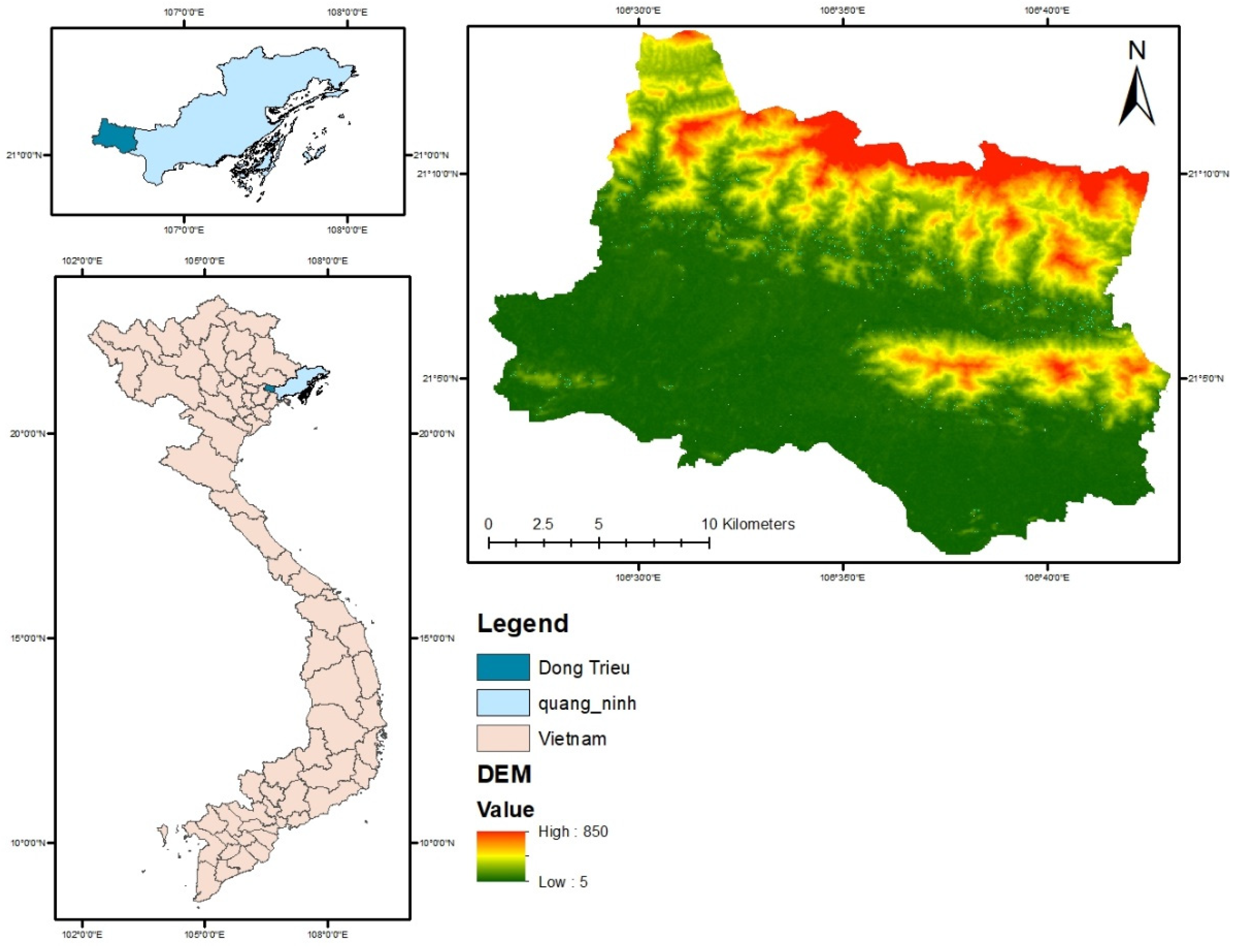
The Dong Trieu district, located between 21°29′04″ and 21°44′55″ N and between 106°33′ and 106°44′57″ E, is a crucial ecological barrier in Quang Ninh province, Vietnam (Figure 1). The topography in Dong Trieu district can be divided into three regions: (1) The northern mountainous region has considerable high terrain; the land in this area is suitable for forest development, fruit tree planting, medicinal plants, and cattle raising. (2) A transitional region has low hills alternating with plains, where the elevation is lower than the mountainous region; the land in this area is suitable for developing perennial crops, industrial crops, and rice cultivation. (3) The southern plain region has the lowest elevation; the land in this area is moderately fertile, mainly formed by alluvium from Kinh Thay and Da Bac rivers, suitable for rice cultivation and freshwater aquaculture. Dong Trieu’s climate is relatively mild. The annual average temperature and humidity are 23 °C and 81%, respectively. The annual rainfall is 1809 mm.
2.2. Data Sources
The land-use distribution maps in 2000, 2010, and 2019 were used in this study, including six land-use types, i.e., Forest, Cropland, Orchards, Waterbody, Built-up, and Barren land. These land-use maps were derived from cloud-free scenes of the Landsat Thematic Mapper-TM (2000 and 2010) and Operational Land Imager-OLI (2019) and classified using ENVI (Version 5.1, Harris Geospatial Solutions, Broomfield, CO, USA), with more than 85% overall accuracy. More details about the production and verification of the land-use maps utilized were described in our previous research [25].
2.3. Land-Use Scenarios for 2030
Four basic land-use utilization scenarios were designed to simulate the land-use distribution pattern changes from 2019 to 2030, i.e., (1) Development as usual (DAU), (2) Build-up Expansion Slowdown (BES), (3) Forest Protection Emphasized (FPE), and (4) Agricultural land Conversion (ALC).
(1) Development as usual
For this basic scenario, the rates of deforestation and built-up expansion were assumed to be 100 ha y−1 and 250 ha y−1, respectively, which correspond to their trend and rate in the period from 2010 to 2019. This represents a baseline scenario without any mitigation policy intervention.
(2) Build-up Expansion Slowdown
In this basic scenario, cases with build-up expansion rates reduced to five levels (200, 150, 100, 50, and 0 ha y−1) were explored to see how the HQ would change if policies of different strengths were enforced to limit the build-up expansion rate.
(3) Forest Protection Emphasized
In this basic scenario, cases with three levels of protection (deforestation rates at 20 and 0 ha y−1 and reforestation rate at 20 ha y−1) were explored to study the effects on improvement in HQ if policies of different strength to protect forest were enforced.
(4) Agricultural Land Conversion
To balance the net changes in Forest, Waterbody, Built-up, and Barren land, the changes in Cropland and Orchards were assumed to have two variations, i.e., orchards preferred and equally distributed, to study the effects of agricultural land-use on HQ and potential farmers’ income. The orchards preferred variation assumed that 75% of the reduced acreage comes from existing Cropland and 25% from existing Orchards when total agricultural land has to decrease. However, when total agricultural land can increase, 75% of the increased acreage becomes Orchards, and the rest, 25%, becomes Cropland. The equally distributed variation assumed that the acreage converted from or to Cropland and Orchards was equally distributed when the acreage of total agricultural land changed.
To simplify the simulation for future scenarios, both the Waterbody and Barren land were assumed to decrease at the rate of 5 ha y−1. Cases simulated in this study are listed in Table 1.
2.4. Land-Use Simulation in 2030
The Dyna-CLUE model (Version 2.0) was employed to simulate the land-use change in 2030 in Dong Trieu District. The distance from road (DFR), distance from main road (DFMR), distance from urban (DFU), distance from water (DFW), elevation, slope and population density, as identified by our previous study [25], were used as driving factors in this study. Based on the opinions of local experts as to the characteristics of land-use in the study region and settings used at other locations [2,26,27,28,29,30,31,32], the change conversion elastic coefficients for Forest, Cropland, Orchards, Waterbody, Built-up, and Barren land were set to 0.7, 0.3, 0.4, 0.7, 1.0, and 0.1, respectively. All land types were permitted to be changed over to one another except the Built-up. The change matrix is expressed in Table 2.
During the model iteration process, the first convergence criterion (average deviation between demanded changes and actually allocated changes) was set at 0.35%. The second convergence criterion (maximum deviation between required changes and actually allocated changes) was set at 3%.
2.5. Habitat Quality Assessment
In this study, we used the land-use maps in 2000, 2010, and 2019 and the land-use maps in 2030 simulated by the Dyna-CLUE model, as described in the previous section, to assess the impact of land-use change on biodiversity and various ecosystem services. The InVEST model (Ver. 3.8.0) is used to produce HQ maps by combining information on LULC suitability and threats to biodiversity. The appraisal of HQ relies upon the accompanying critical boundaries: (1) the different threats probably obliterating HQ and the distances among environments and threat sources, (2) the affectability of each LULC type to every threat, and (3) the suitability of each LULC type for a given territory. The model eventually produces an HQ map showing a worth scope of HQ somewhere in the range of 0 and 1, where 1 demonstrates the most elevated effectiveness for species.
Threat sources and habitat types are the two main criteria needed for the model’s operation. Based on literature reviews and expert interviews [14,15,16,17,18,19,30,33] and according to the characteristics of the research area, threat sources used in this study include Barren land, Built-up, Cropland, road, main road, and urban area (Table 3). The threats to habitat often decrease when the distance between the habitat and threats increases. The model utilized linear or exponential models while calculating the impact of threats to the habitat depending on the specific relationship between the distance–decay degree of a threat and the maximum impact distance to a threat. The impact of threat r that originate in the grid cell y, ry, on habitat in grid cell x is given by irxy and is indicated in the following Equations (1) and (2).
where dxy is the Euclidean distance between the habitat of the location and the threat source; drmax is the maximum effective distance of the threat source r.
The total threat level Dxj of grid cell x in habitat type j can be expressed as:
where R is the total threat factors, is the weight of threat factor r. Yr is the total number of grid cells of the threat factor r in land-use map, ry is the number of stress factors on each grid in the land-use map, and Sjr is the relative sensitivity of land-use type j to threat factor r; βx is the legal accessibility of the grid unit x.
The habitat quality is calculated using the following formula:
where Qxj is the grid x’s habitat quality in land-use type j. Hj is the habitat suitability of land-use type j. K is a half-saturation constant, k constant is 0.5. The z value is the default parameter and is a normalized constant.
3. Results and Discussion
3.1. Changes in Habitat Quality from 2000 to 2019
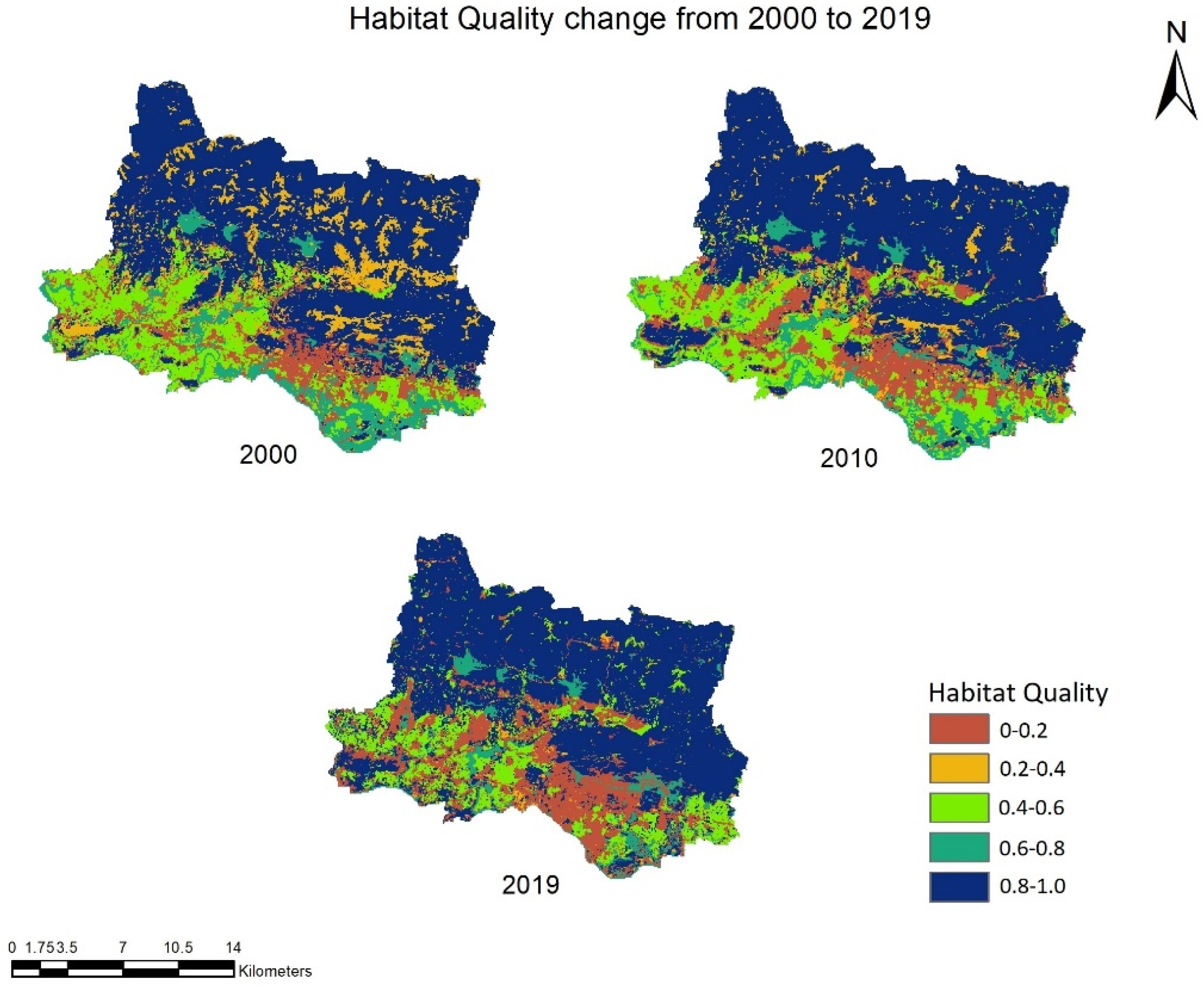
A considerable spatial and temporal variation in HQ was observable in the study area. Figure 2 showed that high-quality areas (HQ > 0.8) were mainly concentrated in the northern and eastern regions, where Forest and Orchards were the primary land-use type. Due to high forest coverage, these regions were not easily affected by cropland and built-up land threats, Good-quality areas (HQ = 0.6−0.8), where Waterbody was the primary land-use type, were scattered in the center and southeastern areas. The moderate quality (HQ = 0.4−0.6) area was mainly located in the southern and western regions where Cropland was the primary land-use type. Low-quality areas (HQ = 0.2−0.4), where Barren land was the primary land-use type, were scattered within the northern forest. Poor-quality areas (HQ < 0.2), where Built-up land was the primary land type, were spread within the regions of moderate quality.
Anthropogenic activities such as urbanization, road construction, and cultivated land greatly aggravated habitat loss and ecosystem degradation [13,14,15,16,17,18,19,33,37,38]. The spatial distribution of HQ in the study area had a gradient distribution pattern of high in the north and low in the south. The middle part was dominated by Orchards but interlaced with Cropland. Hence, the HQ in the central region had a high–low zonal staggered distribution pattern without significant spatial agglomeration.
From 2000 to 2019, the overall HQ of the Dong Trieu district was maintained at a relatively high level due to the large acreage proportion of high-quality habitats (Table 5). The increase in overall average HQ from the 2000–2010 period was due to implementation of forest protection policy in this period. The decrease in HQ to 0.683 in 2019 was mainly due to considerable deforestation for the expansion of Built-up and Orchards [25]. Throughout the past two decades, the acreage proportion of poor-quality habitats increased from 16.8% to 28.5% due to the continuous increase of Built-up areas. Therefore, policies to slow down the Built-up expansion rate and increase forest protection are very important if high environmental quality and overall HQ index are maintained for the Dong Trieu District.
3.2. Land-Use Distribution in 2030
The acreages of various land-use types in Dong Trieu District in 2030 simulated by the Dyna-CLUE model, based on the settings described in Section 2.3, are listed in Table 6. In most cases, Forest and Built-up will be the dominant land-use type in 2030, except cases involving BES5 scenario, and occupied around 37 to 40% and 20 to 26% of the study area, respectively. The acreage of Forest will be decreased to about 14,000 ha if the deforestation rate remains at 100 ha y−1. However, if forest protection policies of different intensities are applied, the Forest area will decline slightly or even increase to approximately 16,000 ha in 2030. The Built-up area can expand to about 10427 ha if the expansion rate does not slow down from the current rate (250 ha y−1). Decreases in Cropland and Orchards were shown in most cases except when Built-up expansion rates were dramatically reduced (BES4) or completely stopped (BES5).
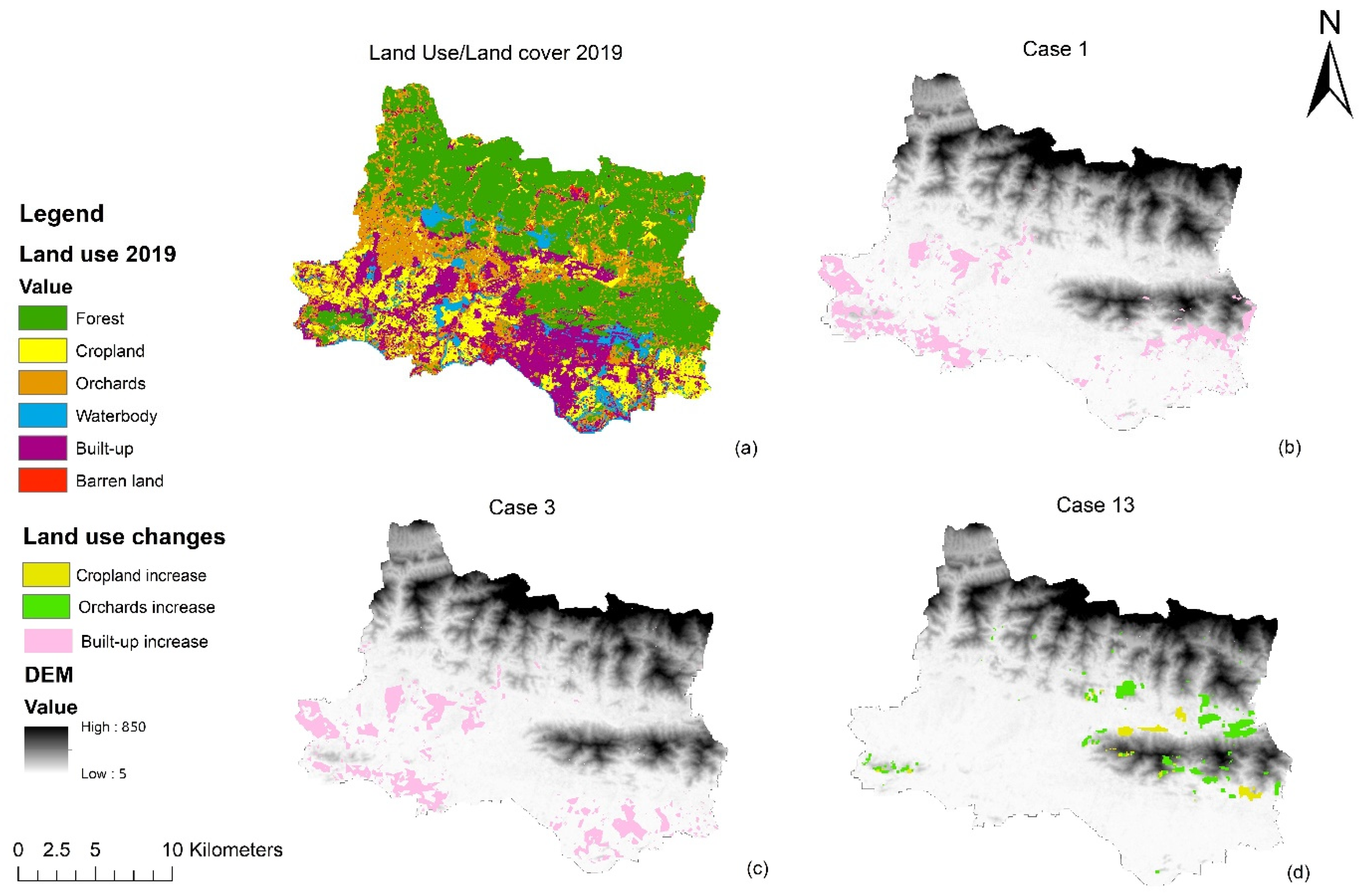
The land-use conversion matrix and locations of major land-use changes from 2019 to 2030 for cases 1, 3, and 13 are shown in Table 7 and Figure 3, respectively. The main changes in case 1 were the significant increase in the Built-up area, by 2700 ha, resulting from the decreases in Forest (1150 ha), Cropland (1090 ha), and Orchards (441 ha) (Table 7, Figure 3b). The Cropland and Orchards in case 3 decreased more than 1869 ha and 802 ha, respectively, which were more than those in case 1 by 800 and 400 ha, respectively (Table 7, Figure 3c). However, the Cropland and Orchards in case 13 showed an increase of 892 and 332 ha, respectively, due to deforestation at the rate of 100 ha y−1 (Table 7, Figure 3d).
The importance of Orchards (fruit trees, perennial plants) in raising farmers’ income and generating revenue by exporting agricultural products has been demonstrated in many sites of Vietnam [39,40,41,42,43]. Especially, research conducted in the northwest of Vietnam indicated that growing fruit trees and perennial plants increased average earnings by 2.4 to 3.5-times that of Cropland [39]. It is expected that the higher the farmers’ income, the more stable social–economic conditions within the region can be established, and better chances to achieve Millennium Development Goals (MDGs) [44,45,46,47]. Dong Trieu district has been selected to produce fruit products meeting Vietnamese Good Agricultural Practices standards, which have contributed to boosting the resident income. For example, custard apple is one of the products which enriched many households in several communes in Dong Trieu district [41]. Therefore, stopping deforestation without slowing down the Built-up expansion rate (cases 3 and 7) can create even severe social and economic unrest due to losing more acreage for Cropland and Orchards.
3.3. Potential Mitigating Strategies
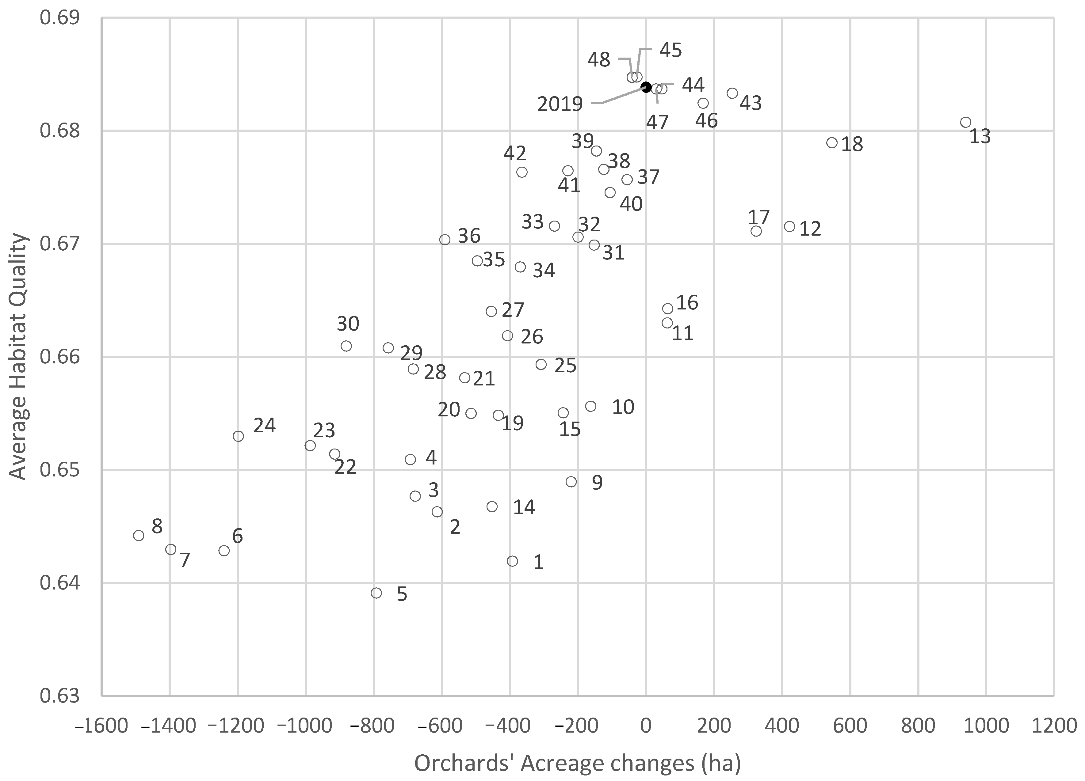
The average HQs and acreage changes in Orchards in 2030 for the various cases simulated are shown in Figure 4. From Figure 4, not only can the effects of different LULC changes on HQ be easily compared, but the impacts on farmers’ livelihood can also be roughly estimated through the net changes in the acreage of Orchards from 2019 by assuming that a positive linear relationship exists between farmers’ total income and the total acreage of Orchards.
As shown in Figure 4, if development continues as usual, the HQ indices could drop to 0.642 and 0.639 by 2030 for case 1 and case 5, respectively. These drops in HQ indices represent a decrease in HQ by 0.041 and 0.046 compared to that of 2019, which is four times faster than the decrease in HQ from 2010 to 2019, and at least two times higher than the decadal HQ decrease found in many regions in China [13,14,16,17]. Besides, 394 ha (5.3%) and 800 ha (10.6%) of Orchards would be lost for cases 1 and 5, respectively. The loss of Orchards may significantly impact farmers’ income and the social–economic conditions in rural areas. The point positions of cases 1 and 5 also indicated that the ALC1 scenario would produce a higher HQ and less Orchard acreage loss than the ALC2 scenario. This is because higher habitat suitability of Orchards was set compared to that of Cropland. Besides, the Orchards’ acreage loss in the ACL1 scenario was less than that in the ALC2 (25% compared to 50%). Therefore, the ALC1 can maintain a higher HQ and reduce Orchard acreage loss than ACL2.
All the three levels of forest protection schemes (FPE1, 2, 3) increased HQ as expected when comparing the point positions of cases 1 to 4 and cases 5 to 8 in Figure 4. For example, the HQ was increased by about 0.009 for case 4 vs. case 1 and 0.005 for case 8 vs. case 5, respectively. However, all the forest protection schemes (FPE1, 2, 3) simulated would cause a decrease in Orchard acreage. For example, the FPE3 (reforestation at 20 ha y−1) scenario would cause nearly 700 ha (9.7%) and 1500 ha (22.1%) loss of Orchards from 2019 to 2030 for cases 4 and 8, respectively. The much more significant loss in Orchards’ acreages than the two DAU scenarios (case 1 and 5) may induce significant impacts on farmers’ income and the social–economic conditions in rural areas. The ALC1 scenario also yields better HQ and less Orchard loss than the ALC2 scenario. However, when comparing the positions of corresponding pairs (i.e., case 1 vs. 5, case 2 vs. 6, case 3 vs. 7, and case 4 vs. 8), the effectiveness of raising HQ by the ALC1 scenario, increased with the strength of the forest protection schemes adopted, was observable. This is due to the higher habitat suitability of Forest compared to that of Orchards.
The effects of five levels of Built-up Expansion Slowdown (BES1, 2, 3, 4, 5) on increasing HQ can be identified by comparing the positions of case 1 with cases 9 to 13, respectively. The big jump in HQ by each level from BES1 to BES5 indicated that slowing down the expansion of the Build-up area was the most effective measure to mitigate the deteriorating HQ in the study area. Besides, the increase in BES strength from level 1 (200 ha y−1) to level 5 (0 ha y−1) could incrementally mitigate the Orchard acreages’ loss, or even increase the Orchards’ acreage. For instance, BES4 (case 12) and BES5 (case 13) increased the acreage of Orchards by 5.3% and 11%, respectively, which may improve the farmer’s revenue and their living standards and contribute to socio-economic stability in the area. The ALC1 plan also creates higher HQ and alleviates less Orchard acreage loss than the ALC2 does when comparing the positions of point sets (i.e., case 9 vs. case 14, case 10 vs. 15, case 11 vs. case 16, case 12 vs. case 17, and case 13 vs. case 18) because of the higher habitat suitability and acreage increase in Orchards in ALC1 scenario as mentioned before. Similar results were also observed when comparing case 5 with cases 14 to 18.
As mentioned above, under the BAU1 scenario (case 1), the HQ would drop to 0.642 and result in a nearly 400 ha Orchard loss in the study area by 2030. Any meaningful proposed mitigation strategies should have the potential to maintain the value of HQ indices higher than 0.65 and the loss of Orchards less than 400 ha. Therefore, cases that could fit these criteria were separated into three groups in the following discussions on potential mitigation strategies for easy comprehension. However, cases assuming a deforestation rate at 100 ha y−1 were excluded, because deforestation at a large scale should be banned in the future, as declared in COP26 [48,49,50].
Group I include cases 43, 44, 46, and 47, which maintained an average HQ not less than 0.68 and resulted in no loss of total acreage of Orchards from 2019. The complete stop built-up expansion (BES5) was the typical scenario assumed in these four cases. Different forest protection scenarios (FPE1, FPE2, and FPE3) and agricultural land conversion scenarios (ALC1 and ALC2) resulted in only slight differences. However, the BES5 scenario may be challenging to achieve in reality because land-use demands for residential areas, industrial zones, and transport system expansion are still required in the regional land-use planning for 2030 [51]. The complete stop built-up expansion may significantly affect the planned socio-economic development of the district. Group II consists of cases 45 and 48 (complete stop built-up expansion), cases 37, 38, 39, and 40 (Built-up expansion rate reduced to 50 ha y−1), and cases 31 and 32 (Built-up expansion rate reduced to 100 ha y−1), which could maintain an average HQ higher than 0.67 and restrict the loss of Orchards to less than 200 ha. Group II provides more potential policy choices than Group I because BES3 and BES4 scenarios have appeared in several cases. Group III comprises cases 33, 34, 41, and 42, which could maintain an HQ higher than 0.66 but with the loss of Orchards areas between 200 and 400 ha. Among these four cases, case 34 was the only case with HQ lower than 0.67. However, cases in Group III provide little stimulus for potential mitigation policies because BES3 (cases 33 and 34) and BES4 (cases 41 and 42) were still the built-up expansion scenarios simulated and had greater Orchards area loss than cases in Group II.
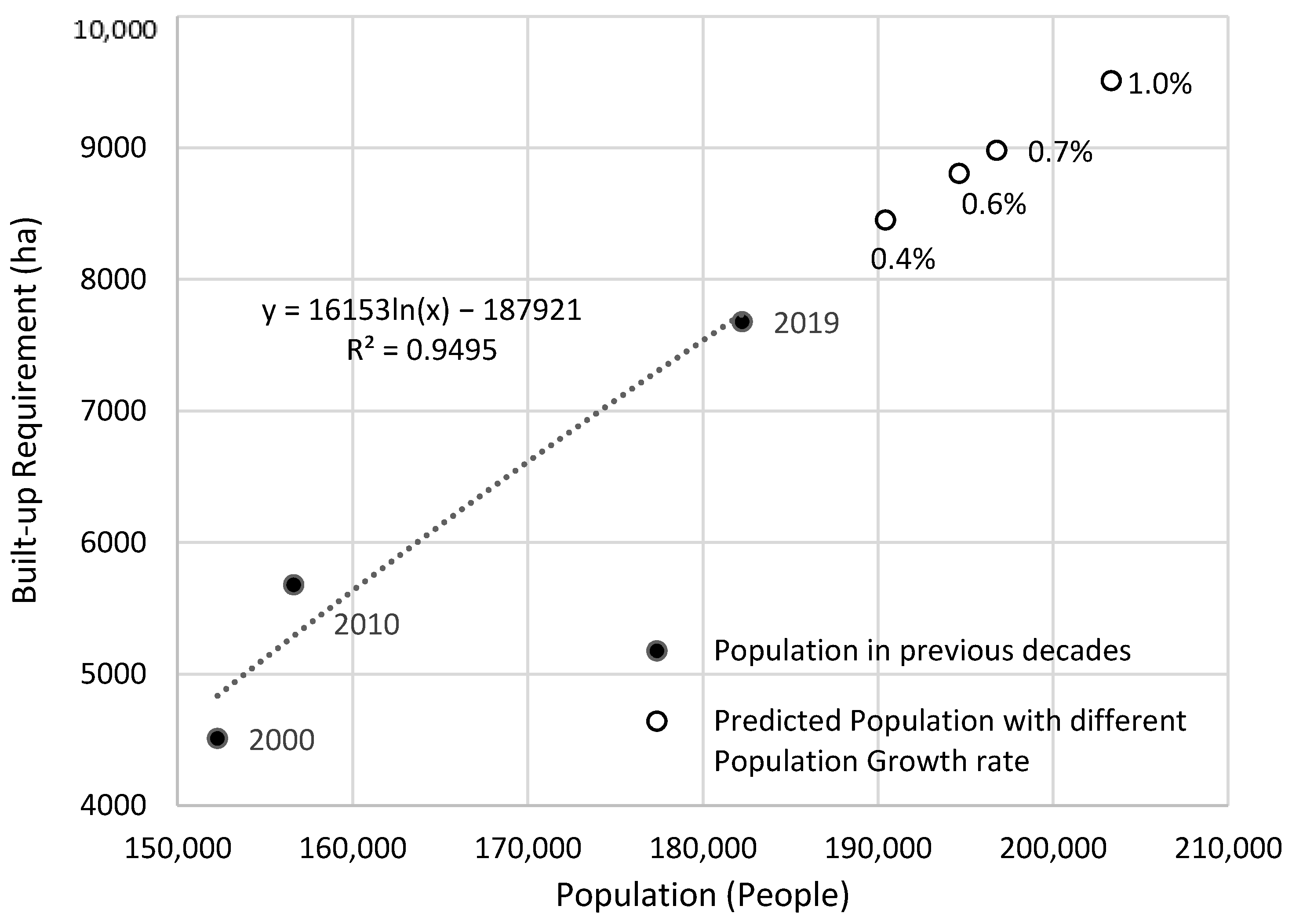
As discussed above, slowing down the Built-up expansion rate to lower than 100 ha y−1 is crucial to avoid significant deterioration of HQ and loss of total acreage in Orchards (and maintain farmers’ livelihood), which implies that the Built-up area cannot exceed 8800 ha in 2030 (Table 6). However, as shown in Figure 5, a logarithmic relationship exists between the Built-up expansion rate and population growth rate from 2000 to 2019. If the logarithmic relationship remains, the population growth rate cannot exceed 0.6% y−1 starting from 2020 to maintain the Built-up area below 8800 ha at 2030. However, the current Vietnam Population Strategy would only reduce the population growth rate from 0.93% to 0.69% during the 2020–2030 period [52]. Therefore, strategies other than controlling the population growth rate should be utilized to constrain the Built-up expansion rate.
When considering the type of built-up land expansion in the urban area in 499 cities from different continents, Mahtta et al. [53] pointed out that expansion upward has more advantages than expansion outward. Although Quang Ninh province already has more than 60 high-rise buildings, most of them are located in Halong city. There is no high-rise building in Dong Trieu district yet. Hence, low buildings in the Dong Trieu district should be converted to high-rise buildings to accommodate the increased population by tapping the existing construction land potential. In that case, the construction land demand in the future can be significantly reduced, and the Built-up area can remain well under 8800 ha even if the population growth rate is still maintained at 0.93%.
Therefore, the already implemented Vietnam Population Strategy by 2030 should be continually enforced to reduce the population growth and the requirements on land-use for accommodations; more guidelines should be followed in designing new policies to mitigate the deteriorating HQ in the study area. Suggested guidelines include (1) changing the urban expansion type from outward to upward to control the Built-up expansion rate, (2) substituting forest-harming industries for the forest-preservation ones to reduce deforestation rate, (3) encouraging Orchards in agricultural land conversion to increase incomes while maintaining higher HQ, (4) practicing better farming technologies to improve crop production and to alleviate potential food security issues due to considerable reduction in Cropland.
Besides the above directions, other approaches that could mitigate the deterioration of HQ should also be implemented. For example, intercropping can be implemented in the Forest and Orchards areas by planting other crops or herbs under the forest or orchard’s shadow as a tree layer. This adds diversity to the farm plant population, improves the HQ, and increases cropping intensity and productivity of the Orchards [54,55,56]. Furthermore, the transportation network that has significant impacts on economic development and urbanization expansion may be expanded much larger than the current system. The greater transportation network disturbances on HQ could be reduced by the Green Infrastructure and Belt and Road Initiative methods that have been used in many southeast Asian countries [57,58]. These methods can increase urban green cover and raise residents’ income.
However, our research focused more on anthropogenic disturbances than on biotic and abiotic factors and assumed that threat factors have impacts on all native species and habitats within the study area without considering possible alternative consequences. We, therefore, recognized that our approach could be improved by selecting more threat factors and assigning more scenarios to increase the versatility of the InVEST-HQ model.
4. Conclusions
Understanding the spatiotemporal changes in HQ is essential for effective land-use planning. Our results indicated that the average HQ and Orchard’s acreage of the Dong Trieu district in 2030 could decrease by 0.044 and about 800 ha, respectively, from those in 2019 if no mitigation measures are made. The deteriorating trend could not only endanger the ecosystem but also cause social and economic unrest.
Stopping deforestation without slowing down the Built-up expansion rate provides little help in keeping the HQ high but can create even more severe social and economic unrest resulting from losing more acreage for Cropland and Orchards. Slowing down Built-up expansion rate to lower than 100 ha y−1 is crucial to avoid significant deterioration in HQ and loss of total acreage in Orchards. The current population growth control policy alone could not slow down the Built-up expansion rate to the required level. More guidelines, such as (1) changing urban expansion type from outward to upward to control the Built-up expansion rate, (2) substituting forest-preservation industries for the forest-harming ones to reduce the deforestation rate, (3) encouraging Orchards for agricultural land conversion to increase incomes while maintaining higher HQ, (4) practicing better farming technologies to improve crop production and to alleviate potential food security issues due to considerable reduction in Cropland, and (5) promoting Green Infrastructure and the Belt and Road Initiative to increase urban green cover for uncertain urban sprawl and traffic system expansion and raise residents’ income, were thus proposed and should be considered seriously in designing the new land-use policies.
Author Contributions
Conceptualization, Y.S.; Data curation, T.T.V.; Formal analysis, T.T.V.; Investigation, T.T.V.; Supervision, Y.S.; Visualization, T.T.V.; Writing—original draft, T.T.V.; Writing—review and editing, Y.S., H.-Y.L. All authors have read and agreed to the published version of the manuscript.
Funding
This research received no external funding.
Institutional Review Board Statement
Not applicable.
Informed Consent Statement
Not applicable.
Data Availability Statement
The data presented in this study are available on request from the corresponding author. The data are not publicly available due to privacy.
Acknowledgments
We gratefully acknowledge the Ministry of Science and Technology, Taiwan for the scholarship support to the first author for her study in Taiwan. We also thank the support of Dong Trieu Division of Natural Resources and Environment, Vietnam for providing the auxiliary data.
Conflicts of Interest
The authors declare no conflict of interest.
References
- Sharp, R.; Tallis, H.; Ricketts, T.; Guerry, A.; Wood, S.A.; Chaplin-Kramer, R.; Nelson, E.; Ennaanay, D.; Wolny, S.; Olwero, N. VEST User’s Guide; The Natural Capital Project: Stanford, CA, USA, 2014. [Google Scholar]
- Terrado, M.; Sabater, S.; Chaplin-Kramer, B.; Mandle, L.; Ziv, G.; Acuña, V. Model development for the assessment of terrestrial and aquatic habitat quality in conservation planning. Sci. Total Environ. 2016, 540, 63–70. [Google Scholar] [CrossRef] [Green Version]
- Sallustio, L.; De Toni, A.; Strollo, A.; Di Febbraro, M.; Gissi, E.; Casella, L.; Geneletti, D.; Munafo, M.; Vizzarri, M.; Marchetti, M. Assessing habitat quality in relation to the spatial distribution of protected areas in Italy. J. Environ. Manag. 2017, 201, 129–137. [Google Scholar] [CrossRef] [PubMed]
- Yohannes, H.; Soromessa, T.; Argaw, M.; Dewan, A. Spatio-temporal changes in habitat quality and linkage with landscape characteristics in the Beressa watershed, Blue Nile basin of Ethiopian highlands. J. Environ. Manag. 2021, 281, 111885. [Google Scholar] [CrossRef] [PubMed]
- Cabral, H.N.; Fonseca, V.F.; Gamito, R.; Gonçalves, C.I.; Costa, J.L.; Erzini, K.; Gonçalves, J.; Martins, J.; Leite, L.; Andrade, J.P.; et al. Ecological quality assessment of transitional waters based on fish assemblages in Portuguese estuaries: The Estuarine Fish Assessment Index (EFAI). Ecol. Indic. 2012, 19, 144–153. [Google Scholar] [CrossRef]
- Meunier, F.D.; Verheyden, C.; Jouventin, P. Bird communities of highway verges: Influence of adjacent habitat and roadside management. Acta Oecologica 1999, 20, 1–13. [Google Scholar] [CrossRef]
- Parris, K.M. Distribution, habitat requirements and conservation of the cascade treefrog (Litoria pearsoniana, Anura: Hylidae). Biol. Conserv. 2001, 99, 285–292. [Google Scholar] [CrossRef]
- Arenas-Castro, S.; Sillero, N. Cross-scale monitoring of habitat suitability changes using satellite time series and ecological niche models. Sci. Total Environ. 2021, 784, 147172. [Google Scholar] [CrossRef] [PubMed]
- Cao, Y.; Li, G.; Cao, Y.; Wang, J.; Fang, X.; Zhou, L.; Liu, Y. Distinct types of restructuring scenarios for rural settlements in a heterogeneous rural landscape: Application of a clustering approach and ecological niche modeling. Habitat Int. 2020, 104, 102248. [Google Scholar] [CrossRef]
- Mwakapeje, E.R.; Ndimuligo, S.A.; Mosomtai, G.; Ayebare, S.; Nyakarahuka, L.; Nonga, H.E.; Mdegela, R.H.; Skjerve, E. Ecological niche modeling as a tool for prediction of the potential geographic distribution of Bacillus anthracis spores in Tanzania. Int. J. Infect. Dis. 2019, 79, 142–151. [Google Scholar] [CrossRef] [Green Version]
- Fish, U.; Service, W. Habitat Evaluation Procedures; Fish & Wildlife Services: Washington, DC, USA, 1976. [Google Scholar]
- Zeng, X.; Tanaka, K.R.; Chen, Y.; Wang, K.; Zhang, S. Gillnet data enhance performance of rockfishes habitat suitability index model derived from bottom-trawl survey data: A case study with Sebasticus marmoratus. Fish. Res. 2018, 204, 189–196. [Google Scholar] [CrossRef]
- Zhang, H.; Wu, F.; Zhang, Y.; Han, S.; Liu, Y. Spatial and temporal changes of habitat quality in Jiangsu Yancheng Wetland National Nature Reserve-Rare birds of China. Appl. Ecol. Environ. Res. 2019, 17, 4807–4821. [Google Scholar] [CrossRef]
- Chen, M.; Bai, Z.; Wang, Q.; Shi, Z. Habitat quality effect and driving mechanism of land use transitions: A case study of Henan water source area of the middle route of the south-to-north water transfer project. Land 2021, 10, 796. [Google Scholar] [CrossRef]
- Wu, L.; Sun, C.; Fan, F. Estimating the Characteristic Spatiotemporal Variation in Habitat Quality Using the InVEST Model—A Case Study from Guangdong–Hong Kong–Macao Greater Bay Area. Remote Sens. 2021, 13, 1008. [Google Scholar] [CrossRef]
- Li, M.; Zhou, Y.; Xiao, P.; Tian, Y.; Huang, H.; Xiao, L. Evolution of Habitat Quality and Its Topographic Gradient Effect in Northwest Hubei Province from 2000 to 2020 Based on the InVEST Model. Land 2021, 10, 857. [Google Scholar] [CrossRef]
- Chu, L.; Sun, T.; Wang, T.; Li, Z.; Cai, C. Evolution and prediction of landscape pattern and habitat quality based on CA-Markov and InVEST model in Hubei section of Three Gorges Reservoir Area (TGRA). Sustainability 2018, 10, 3854. [Google Scholar] [CrossRef] [Green Version]
- Xu, L.; Chen, S.S.; Xu, Y.; Li, G.; Su, W. Impacts of land-use change on habitat quality during 1985–2015 in the Taihu Lake Basin. Sustainability 2019, 11, 3513. [Google Scholar] [CrossRef] [Green Version]
- Berta Aneseyee, A.; Noszczyk, T.; Soromessa, T.; Elias, E. The InVEST habitat quality model associated with land use/cover changes: A qualitative case study of the Winike Watershed in the Omo-Gibe Basin, Southwest Ethiopia. Remote Sens. 2020, 12, 1103. [Google Scholar] [CrossRef] [Green Version]
- Castella, J.-C.; Kam, S.P.; Quang, D.D.; Verburg, P.H.; Hoanh, C.T. Combining top-down and bottom-up modelling approaches of land use/cover change to support public policies: Application to sustainable management of natural resources in northern Vietnam. Land Use Policy 2007, 24, 531–545. [Google Scholar] [CrossRef]
- Verburg, P.H.; Kok, K.; Pontius, R.G.; Veldkamp, A. Modeling land-use and land-cover change. In Land-Use and Land-Cover Change. Global Change—The IGBP Series; Lambin, E.F., Geist, H., Eds.; Springer: Berlin/Heidelberg, Germany, 2006; pp. 117–135. [Google Scholar]
- Verburg, P.H.; Soepboer, W.; Veldkamp, A.; Limpiada, R.; Espaldon, V.; Mastura, S.S. Modeling the spatial dynamics of regional land use: The CLUE-S model. Env. Manag. 2002, 30, 391–405. [Google Scholar] [CrossRef]
- Lippe, M.; Hilger, T.; Sudchalee, S.; Wechpibal, N.; Jintrawet, A.; Cadisch, G. Simulating stakeholder-based land-use change scenarios and their implication on above-ground carbon and environmental management in northern Thailand. Land 2017, 6, 85. [Google Scholar] [CrossRef] [Green Version]
- Adhikari, R.K.; Mohanasundaram, S.; Shrestha, S. Impacts of land-use changes on the groundwater recharge in the Ho Chi Minh city, Vietnam. Environ. Res. 2020, 185, 109440. [Google Scholar] [CrossRef] [PubMed]
- Vu, T.-T.; Shen, Y. Land-use and land-cover changes in dong trieu district, vietnam, during past two decades and their driving forces. Land 2021, 10, 798. [Google Scholar] [CrossRef]
- Henríquez-Dole, L.; Usón, T.J.; Vicuña, S.; Henríquez, C.; Gironás, J.; Meza, F. Integrating strategic land use planning in the construction of future land use scenarios and its performance: The Maipo River Basin, Chile. Land Use Policy 2018, 78, 353–366. [Google Scholar] [CrossRef]
- Lü, D.; Gao, G.; Lü, Y.; Ren, Y.; Fu, B. An effective accuracy assessment indicator for credible land use change modelling: Insights from hypothetical and real landscape analyses. Ecol. Indic. 2020, 117, 106552. [Google Scholar] [CrossRef]
- Otto, C.R.; Roth, C.L.; Carlson, B.L.; Smart, M.D. Land-use change reduces habitat suitability for supporting managed honey bee colonies in the Northern Great Plains. Proc. Natl. Acad. Sci. USA 2016, 113, 10430–10435. [Google Scholar] [CrossRef] [Green Version]
- Sahoo, S.; Sil, I.; Dhar, A.; Debsarkar, A.; Das, P.; Kar, A. Future scenarios of land-use suitability modeling for agricultural sustainability in a river basin. J. Clean. Prod. 2018, 205, 313–328. [Google Scholar] [CrossRef]
- Tang, F.; Fu, M.; Wang, L.; Zhang, P. Land-use change in Changli County, China: Predicting its spatio-temporal evolution in habitat quality. Ecol. Indic. 2020, 117, 106719. [Google Scholar] [CrossRef]
- Wang, Y.; Chao, B.; Dong, P.; Zhang, D.; Yu, W.; Hu, W.; Ma, Z.; Chen, G.; Liu, Z.; Chen, B. Simulating spatial change of mangrove habitat under the impact of coastal land use: Coupling MaxEnt and Dyna-CLUE models. Sci. Total Environ. 2021, 788, 147914. [Google Scholar] [CrossRef]
- Zhu, C.; Zhang, X.; Zhou, M.; He, S.; Gan, M.; Yang, L.; Wang, K. Impacts of urbanization and landscape pattern on habitat quality using OLS and GWR models in Hangzhou, China. Ecol. Indic. 2020, 117, 106654. [Google Scholar] [CrossRef]
- Yang, Y. Evolution of habitat quality and association with land-use changes in mountainous areas: A case study of the Taihang Mountains in Hebei Province, China. Ecol. Indic. 2021, 129, 107967. [Google Scholar] [CrossRef]
- Lindenmayer, D.; Hobbs, R.J.; Montague-Drake, R.; Alexandra, J.; Bennett, A.; Burgman, M.; Cale, P.; Calhoun, A.; Cramer, V.; Cullen, P. A checklist for ecological management of landscapes for conservation. Ecol. Lett. 2008, 11, 78–91. [Google Scholar] [CrossRef] [PubMed]
- Ruzicka, M.; Misovicova, R. The general and special principles in landscape ecology. Ekologia 2009, 28, 1–6. [Google Scholar] [CrossRef]
- Wang, H.; Tang, L.; Qiu, Q.; Chen, H. Assessing the impacts of urban expansion on habitat quality by combining the concepts of land use, landscape, and habitat in two urban agglomerations in China. Sustainability 2020, 12, 4346. [Google Scholar] [CrossRef]
- Rahman, M.M.; Szabó, G. Impact of land use and land cover changes on urban ecosystem service value in Dhaka, Bangladesh. Land 2021, 10, 793. [Google Scholar] [CrossRef]
- Tang, J.; Li, Y.; Cui, S.; Xu, L.; Ding, S.; Nie, W. Linking land-use change, landscape patterns, and ecosystem services in a coastal watershed of southeastern China. Glob. Ecol. Conserv. 2020, 23, e01177. [Google Scholar] [CrossRef]
- Do, V. Fruit tree-based agroforestry systems for smallholder farmers in Northwest Vietnam—A quantitative and qualitative assessment. Land 2020, 9, 451. [Google Scholar] [CrossRef]
- Nguyen, P.; Nguyen, S. Southern Provinces Promote Sustainable Development of Fruit Tree Farming. Available online: https://en.nhandan.vn/business/item/10717702-southern-provinces-promote-sustainable-development-of-fruit-tree-farming.html (accessed on 12 December 2021).
- Nongnghiep.vn. Dong Trieu Custard-Apples. Available online: http://www.en.trithuckhoahoc.vn/default.aspx?tabid=230&NDID=14257 (accessed on 12 December 2021).
- Nhandan.vn. Vietnamese Fruits Reach Out to the World. Available online: https://www.agroberichtenbuitenland.nl/actueel/nieuws/2020/07/30/vietnamese-fruits-reach-out-to-the-world (accessed on 12 December 2021).
- Vietnamnews.vn. Dak Lak Farmers Boost Income with Fruit Trees. Available online: https://vietnamnews.vn/society/274507/dak-lak-farmers-boost-income-with-fruit-trees.html (accessed on 12 December 2021).
- Le, Q.B. What Has Made Vietnam a Poverty Reduction Success Story; Oxfam International: Nairobi, Kenya, 2008; Volume 29. [Google Scholar]
- Mbow, C.; van Noordwijk, M.; Prabhu, R.; Simons, T. Knowledge gaps and research needs concerning agroforestry’s contribution to sustainable development goals in Africa. Curr. Opin. Environ. Sustain. 2014, 6, 162–170. [Google Scholar] [CrossRef] [Green Version]
- Montagnini, F.; Metzel, R.N. The Contribution of Agroforestry to Sustainable Development Goal 2: End Hunger, Achieve Food Security and Improved Nutrition, and Promote Sustainable Agriculture; Springer International Publishing AG: Cham, Switzerland, 2017; pp. 11–45. [Google Scholar]
- Sok, S. Pro-poor growth development and income inequality: Poverty-related Millennium Development Goal (MDG 1) on banks of the Lower Mekong Basin in Cambodia. World Dev. Perspect. 2017, 7–8, 1–8. [Google Scholar] [CrossRef]
- Arora, N.K.; Mishra, I. COP26: More challenges than achievements. Environ. Sustain. 2021, 4, 585–588. [Google Scholar] [CrossRef]
- Issa, R.; Krzanowski, J. Finding Hope in COP26. Available online: https://0-www-bmj-com.brum.beds.ac.uk/content/375/bmj.n2940.full (accessed on 30 November 2021).
- Mountford, H.; Waskow, D.; Srouji, J.; Seymour, F.; Gonzalez, L.; Gajjar, C. Top Takeaways from the UN World Leaders Summit at COP26. Available online: https://www.wri.org/insights/top-takeaways-un-world-leaders-summit-cop26 (accessed on 20 November 2021).
- Quang Ninh Provincial People’s Committee. Land Use Planning for 2021–2030 Period in Dong Trieu District. Available online: https://www.quangninh.gov.vn/so/sokhdt/Trang/ChiTietTinTuc.aspx?nid=1229 (accessed on 21 May 2021).
- Minister, P. Decision No. 1679/QD-TTg 2019 Approving Vietnam’s Strategy for Population toward 2030; National Political Publishing House: Hanoi, Vietnam, 2019. [Google Scholar]
- Mahtta, R.; Mahendra, A.; Seto, K.C. Building up or spreading out? Typologies of urban growth across 478 cities of 1 million+. Environ. Res. Lett. 2019, 14, 124077. [Google Scholar] [CrossRef] [Green Version]
- Morugán-Coronado, A.; Linares, C.; Gómez-López, M.D.; Faz, Á.; Zornoza, R. The impact of intercropping, tillage and fertilizer type on soil and crop yield in fruit orchards under Mediterranean conditions: A meta-analysis of field studies. Agric. Syst. 2020, 178, 102736. [Google Scholar] [CrossRef]
- Srivastava, A.K.; Huchche, A.D.; Ram, L.; Singh, S. Yield prediction in intercropped versus monocropped citrus orchards. Sci. Hortic. 2007, 114, 67–70. [Google Scholar] [CrossRef]
- Zhu, L.; He, J.; Tian, Y.; Li, X.; Li, Y.; Wang, F.; Qin, K.; Wang, J. Intercropping wolfberry with gramineae plants improves productivity and soil quality. Sci. Hortic. 2022, 292, 110632. [Google Scholar] [CrossRef]
- Ng, L.S.; Campos-Arceiz, A.; Sloan, S.; Hughes, A.C.; Tiang, D.C.F.; Li, B.V.; Lechner, A.M. The scale of biodiversity impacts of the belt and road initiative in Southeast Asia. Biol. Conserv. 2020, 248, 108691. [Google Scholar] [CrossRef]
- Kuah, K.E. Traditional Chinese herbal medicine as cultural power along the Southeast Asian belt and road corridor. Asian J. Soc. Sci. 2021, 49, 225–233. [Google Scholar] [CrossRef]
Figure 1.
Location and digital elevation model of the study area.

Figure 2.
Spatial distribution and change in habitat quality in the study area.

Figure 3.
LULC at 2019 and land-use changes from 2019 to 2030 for three simulated cases: (a) Land use/Land cover in 2019, (b) Built-up increase by 2030 in case 1, (c) Built-up increase by 2030 in case 3, and (d) Cropland and Orchards increase by 2030 in case 13.
Figure 3.
LULC at 2019 and land-use changes from 2019 to 2030 for three simulated cases: (a) Land use/Land cover in 2019, (b) Built-up increase by 2030 in case 1, (c) Built-up increase by 2030 in case 3, and (d) Cropland and Orchards increase by 2030 in case 13.

Figure 4.
Changes in habitat quality and acreage of Orchards of various simulated cases.

Figure 5.
Relationship between Built-up requirement and population.


Table 1.
Acreage changes per year of the six land-use types used to simulate the land-use distribution maps in 2030.
Table 1.
Acreage changes per year of the six land-use types used to simulate the land-use distribution maps in 2030.
| Case | Forest | Cropland | Orchards | Waterbody | Built-Up | Barren Land | Scenarios Simulated * |
|---|---|---|---|---|---|---|---|
| 1 | −100.0 | −105.0 | −35.0 | −5.0 | 250.0 | −5.0 | DAU+ALC1 |
| 2 | −20.0 | −165.0 | −55.0 | −5.0 | 250.0 | −5.0 | FPE1+ALC1 |
| 3 | 0.0 | −180.0 | −60.0 | −5.0 | 250.0 | −5.0 | FPE2+ALC1 |
| 4 | 20.0 | −195.0 | −65.0 | −5.0 | 250.0 | −5.0 | FPE3+ALC1 |
| 5 | −100.0 | −70.0 | −70.0 | −5.0 | 250.0 | −5.0 | DAU+ALC2 |
| 6 | −20.0 | −110.0 | −110.0 | −5.0 | 250.0 | −5.0 | FPE1+ALC2 |
| 7 | 0.0 | −120.0 | −120.0 | −5.0 | 250.0 | −5.0 | FPE2+ALC2 |
| 8 | 20.0 | −130.0 | −130.0 | −5.0 | 250.0 | −5.0 | FPE3+ALC2 |
| 9 | −100.0 | −67.5 | −22.5 | −5.0 | 200.0 | −5.0 | BES1+ALC1 |
| 10 | −100.0 | −30.0 | −10.0 | −5.0 | 150.0 | −5.0 | BES2+ALC1 |
| 11 | −100.0 | 2.5 | 7.5 | −5.0 | 100.0 | −5.0 | BES3+ALC1 |
| 12 | −100.0 | 15.0 | 45.0 | −5.0 | 50.0 | −5.0 | BES4+ALC1 |
| 13 | −100.0 | 27.5 | 82.5 | −5.0 | 0.0 | −5.0 | BES5+ALC1 |
| 14 | −100.0 | −45.0 | −45.0 | −5.0 | 200.0 | −5.0 | BES1+ALC2 |
| 15 | −100.0 | −20.0 | −20.0 | −5.0 | 150.0 | −5.0 | BES2+ALC2 |
| 16 | −100.0 | 5.0 | 5.0 | −5.0 | 100.0 | −5.0 | BES3+ALC2 |
| 17 | −100.0 | 30.0 | 30.0 | −5.0 | 50.0 | −5.0 | BES4+ALC2 |
| 18 | −100.0 | 55.0 | 55.0 | −5.0 | 0.0 | −5.0 | BES5+ALC2 |
| 19 | −20.0 | −127.5 | −42.5 | −5.0 | 200.0 | −5.0 | BES1+FPE1+ALC1 |
| 20 | 0.0 | −142.5 | −47.5 | −5.0 | 200.0 | −5.0 | BES1+FPE2+ALC1 |
| 21 | 20.0 | −157.5 | −52.5 | −5.0 | 200.0 | −5.0 | BES1+FPE3+ALC1 |
| 22 | −20.0 | −85.0 | −85.0 | −5.0 | 200.0 | −5.0 | BES1+FPE1+ALC2 |
| 23 | 0.0 | −95.0 | −95.0 | −5.0 | 200.0 | −5.0 | BES1+FPE2+ALC2 |
| 24 | 20.0 | −105.0 | −105.0 | −5.0 | 200.0 | −5.0 | BES1+FPE3+ALC2 |
| 25 | −20.0 | −90.0 | −30.0 | −5.0 | 150.0 | −5.0 | BES2+FPE1+ALC1 |
| 26 | 0.0 | −105.0 | −35.0 | −5.0 | 150.0 | −5.0 | BES2+FPE2+ALC1 |
| 27 | 20.0 | −120.0 | −40.0 | −5.0 | 150.0 | −5.0 | BES2+FPE3+ALC1 |
| 28 | −20.0 | −60.0 | −60.0 | −5.0 | 150.0 | −5.0 | BES2+FPE1+ALC2 |
| 29 | 0.0 | −70.0 | −70.0 | −5.0 | 150.0 | −5.0 | BES2+FPE2+ALC2 |
| 30 | 20.0 | −80.0 | −80.0 | −5.0 | 150.0 | −5.0 | BES2+FPE3+ALC2 |
| 31 | −20.0 | −52.5 | −17.5 | −5.0 | 100.0 | −5.0 | BES3+FPE1+ALC1 |
| 32 | 0.0 | −67.5 | −22.5 | −5.0 | 100.0 | −5.0 | BES3+FPE2+ALC1 |
| 33 | 20.0 | −82.5 | −27.5 | −5.0 | 100.0 | −5.0 | BES3+FPE3+ALC1 |
| 34 | −20.0 | −35.0 | −35.0 | −5.0 | 100.0 | −5.0 | BES3+FPE1+ALC2 |
| 35 | 0.0 | −45.0 | −45.0 | −5.0 | 100.0 | −5.0 | BES3+FPE2+ALC2 |
| 36 | 20.0 | −55.0 | −55.0 | −5.0 | 100.0 | −5.0 | BES3+FPE3+ALC2 |
| 37 | −20.0 | −15.0 | −5.0 | −5.0 | 50.0 | −5.0 | BES4+FPE1+ALC1 |
| 38 | 0.0 | −30.0 | −10.0 | −5.0 | 50.0 | −5.0 | BES4+FPE2+ALC1 |
| 39 | 20.0 | −45.0 | −15.0 | −5.0 | 50.0 | −5.0 | BES4+FPE3+ALC1 |
| 40 | −20.0 | −10.0 | −10.0 | −5.0 | 50.0 | −5.0 | BES4+FPE1+ALC2 |
| 41 | 0.0 | −20.0 | −20.0 | −5.0 | 50.0 | −5.0 | BES4+FPE2+ALC2 |
| 42 | 20.0 | −30.0 | −30.0 | −5.0 | 50.0 | −5.0 | BES4+FPE3+ALC2 |
| 43 | −20.0 | 7.5 | 22.5 | −5.0 | 0.0 | −5.0 | BES5+FPE1+ALC1 |
| 44 | 0.0 | 2.5 | 7.5 | −5.0 | 0.0 | −5.0 | BES5+FPE2+ALC1 |
| 45 | 20.0 | −7.5 | −2.5 | −5.0 | 0.0 | −5.0 | BES5+FPE3+ALC1 |
| 46 | −20.0 | 15.0 | 15.0 | −5.0 | 0.0 | −5.0 | BES5+FPE1+ALC2 |
| 47 | 0.0 | 5.0 | 5.0 | −5.0 | 0.0 | −5.0 | BES5+FPE2+ALC2 |
| 48 | 20.0 | −5.0 | −5.0 | −5.0 | 0.0 | −5.0 | BES5+FPE3+ALC2 |
* FPE1, 2, 3 represents deforestation rate at 20 and 0 ha y−1 and reforestation rate at 20 ha y−1, respectively; BES1, 2, 3, 4, and 5 represents built-up expansion slowed down to the rate of 200, 150, 100, 50, and 0 ha y−1, respectively, and ALC1 and ALC2 represent orchards preferred and equally distributed, respectively.
Table 2.
Land-use change matrix.
| Forest | Cropland | Orchards | Waterbody | Built-Up | Barren Land | |
|---|---|---|---|---|---|---|
| Forest | 1 * | 1 | 1 | 0 | 1 | 1 |
| Cropland | 1 | 1 | 1 | 1 | 1 | 0 |
| Orchards | 1 | 1 | 1 | 0 | 1 | 0 |
| Waterbody | 0 | 1 | 1 | 1 | 1 | 0 |
| Built-up | 0 | 0 | 0 | 0 | 1 | 0 |
| Barren land | 1 | 1 | 1 | 1 | 1 | 1 |
* 1 and 0 represents changes allowed and changes not allowed, respectively.
Table 3.
Weights and maximum impact distances of threat factors.
| Threat Factors | Maximum Impact Distance (km) | Weight | Decay Type |
|---|---|---|---|
| Barren land | 8.8 | 0.5 | Linear |
| Built-up | 2.0 | 1.0 | Exponential |
| Cropland | 7.6 | 0.7 | Linear |
| Main road | 11.9 | 1.0 | Linear |
| Road | 3.7 | 0.7 | Linear |
| Urban | 12.2 | 1.0 | Exponential |
Table 4.
Relative sensitivity of different land types to threat factors.
| LULC | Habitat Suitability | Threats | |||||
|---|---|---|---|---|---|---|---|
| Barren Land | Built-Up | Cropland | Main Road | Road | Urban | ||
| Forest | 0.90 | 0.55 | 0.90 | 0.85 | 0.75 | 0.65 | 1.00 |
| Cropland | 0.60 | 0.30 | 0.35 | 0.65 | 0.60 | 0.50 | 0.60 |
| Orchards | 0.85 | 0.50 | 0.35 | 0.90 | 0.75 | 0.65 | 1.00 |
| Waterbody | 0.70 | 0.45 | 0.75 | 0.85 | 0.70 | 0.40 | 0.85 |
| Built-up | 0.15 | 0.60 | 1.00 | 0.78 | 0.80 | 0.70 | 0.68 |
| Barren land | 0.33 | 0.50 | 0.42 | 0.29 | 0.70 | 0.60 | 0.61 |
Table 5.
Changes in the distribution of each habitat level and overall averaged HQ from 2000 to 2019.
Table 5.
Changes in the distribution of each habitat level and overall averaged HQ from 2000 to 2019.
| HQ | 2000 | 2010 | 2019 | 2000–2010 (ha) | 2010–2019 (ha) | 2000–2019 (ha) | |||
|---|---|---|---|---|---|---|---|---|---|
| (ha) | (%) | (ha) | (%) | (ha) | (%) | ||||
| >0.8 | 21,091.2 | 53.6 | 21,949.3 | 55.8 | 23,398.2 | 59.4 | 858.1 | 1448.9 | 2307.0 |
| 0.6–0.8 | 3398.2 | 8.6 | 3339.5 | 8.5 | 2250.5 | 5.7 | −58.7 | −1089.0 | −1147.7 |
| 0.4–0.6 | 6310.4 | 16.0 | 6463.5 | 16.4 | 5560.9 | 14.1 | 153.1 | −902.6 | −749.5 |
| 0.2–0.4 | 4050.4 | 10.3 | 1930.5 | 4.9 | 473.9 | 1.2 | −2119.9 | −1456.6 | −3576.5 |
| 0.0–0.2 | 4510.3 | 11.5 | 5677.7 | 14.4 | 7677.1 | 19.5 | 1167.4 | 1999.3 | 3166.8 |
| Overall | 0.684 | 0.691 | 0.683 | ||||||
Table 6.
Acreages of different land-use types under various scenarios simulated.
| Case | Forest | Cropland | Orchards | Water Body | Built-Up | Barren-Land | Scenarios Simulated |
|---|---|---|---|---|---|---|---|
| 1 | 14,758.9 | 4427.1 | 7154.6 | 2198.4 | 10,418.2 | 403.4 | DAU+ALC1 |
| 2 | 15,660.2 | 3684.6 | 6934.3 | 2187.8 | 10,478.7 | 416.3 | FPE1+ALC1 |
| 3 | 15,876.3 | 3619.6 | 6858.9 | 2166.1 | 10,432.8 | 406.9 | FPE2+ALC1 |
| 4 | 16,117.0 | 3419.8 | 6855.4 | 2213.2 | 10,341.2 | 415.3 | FPE3+ALC1 |
| 5 | 14,759.0 | 4811.5 | 6755.3 | 2209.2 | 10,414.4 | 412.6 | DAU+ALC2 |
| 6 | 15,650.7 | 4342.8 | 6308.1 | 2212.9 | 10,431.4 | 416.1 | FPE1+ALC2 |
| 7 | 15,868.1 | 4234.6 | 6151.9 | 2211.7 | 10,479.5 | 416.2 | FPE2+ALC2 |
| 8 | 16,073.6 | 4139.9 | 6057.1 | 2215.4 | 10,451.7 | 424.3 | FPE3+ALC2 |
| 9 | 14,757.0 | 4762.5 | 7328.3 | 2224.0 | 9869.0 | 421.0 | BES1+ALC1 |
| 10 | 14,759.0 | 5249.2 | 7386.0 | 2227.9 | 9319.0 | 420.8 | BES2+ALC1 |
| 11 | 14,762.3 | 5563.4 | 7610.9 | 2233.4 | 8775.4 | 416.5 | BES3+ALC1 |
| 12 | 14,807.1 | 5728.8 | 7970.5 | 2188.2 | 8243.9 | 423.5 | BES4+ALC1 |
| 13 | 14,750.3 | 5861.3 | 8423.8 | 2220.6 | 7677.0 | 427.6 | BES5+ALC1 |
| 14 | 14,762.3 | 4969.4 | 7095.5 | 2187.4 | 9926.4 | 420.9 | BES1+ALC2 |
| 15 | 14,768.8 | 5332.3 | 7305.0 | 2211.7 | 9333.3 | 410.8 | BES2+ALC2 |
| 16 | 14,777.5 | 5623.3 | 7612.3 | 2226.4 | 8699.6 | 422.9 | BES3+ALC2 |
| 17 | 14,820.7 | 5862.7 | 7872.2 | 2163.1 | 8223.2 | 420.1 | BES4+ALC2 |
| 18 | 14,747.6 | 6164.7 | 8094.6 | 2233.6 | 7699.8 | 421.6 | BES5+ALC2 |
| 19 | 15,658.2 | 4117.6 | 7114.1 | 2217.4 | 9837.0 | 417.6 | BES1+FPE1+ALC1 |
| 20 | 15,841.8 | 3936.4 | 7033.8 | 2211.7 | 9865.8 | 472.4 | BES1+FPE2+ALC1 |
| 21 | 16,092.5 | 3823.6 | 7015.6 | 2211.7 | 9746.2 | 472.4 | BES1+FPE3+ALC1 |
| 22 | 15,622.3 | 4604.9 | 6633.6 | 2216.9 | 9813.2 | 471.1 | BES1+FPE1+ALC2 |
| 23 | 15,797.2 | 4517.8 | 6561.3 | 2212.9 | 9856.4 | 416.3 | BES1+FPE2+ALC2 |
| 24 | 16,087.6 | 4420.5 | 6349.8 | 2224.0 | 9861.1 | 418.9 | BES1+FPE3+ALC2 |
| 25 | 15,486.2 | 4573.9 | 7240.1 | 2222.2 | 9366.4 | 473.1 | BES2+FPE1+ALC1 |
| 26 | 15,852.0 | 4360.5 | 7141.2 | 2222.0 | 9363.9 | 422.4 | BES2+FPE2+ALC1 |
| 27 | 16,078.8 | 4261.4 | 7093.4 | 2211.7 | 9300.8 | 415.9 | BES2+FPE3+ALC1 |
| 28 | 15,659.3 | 4873.8 | 6864.0 | 2209.2 | 9339.8 | 415.8 | BES2+FPE1+ALC2 |
| 29 | 15,868.7 | 4774.0 | 6790.6 | 2215.4 | 9242.7 | 470.5 | BES2+FPE2+ALC2 |
| 30 | 16,085.4 | 4640.9 | 6667.0 | 2215.4 | 9338.4 | 414.8 | BES2+FPE3+ALC2 |
| 31 | 15,653.5 | 5011.7 | 7395.6 | 2211.7 | 8670.0 | 419.4 | BES3+FPE1+ALC1 |
| 32 | 15,868.4 | 4786.8 | 7348.7 | 2211.7 | 8724.0 | 422.4 | BES3+FPE2+ALC1 |
| 33 | 16,076.0 | 4626.5 | 7279.4 | 2219.2 | 8742.2 | 418.8 | BES3+FPE3+ALC1 |
| 34 | 15,636.6 | 5195.4 | 7178.8 | 2219.7 | 8707.2 | 424.3 | BES3+FPE1+ALC2 |
| 35 | 15,859.2 | 5077.1 | 7052.5 | 2216.2 | 8744.1 | 412.8 | BES3+FPE2+ALC2 |
| 36 | 16,090.6 | 4998.6 | 6957.1 | 2218.2 | 8677.0 | 420.5 | BES3+FPE3+ALC2 |
| 37 | 15,638.1 | 5401.5 | 7492.5 | 2226.6 | 8177.6 | 425.6 | BES4+FPE1+ALC1 |
| 38 | 15,842.4 | 5236.7 | 7424.3 | 2235.5 | 8200.4 | 422.6 | BES4+FPE2+ALC1 |
| 39 | 16,063.4 | 5057.6 | 7402.6 | 2226.6 | 8195.8 | 416.0 | BES4+FPE3+ALC1 |
| 40 | 15,582.1 | 5454.7 | 7442.9 | 2241.8 | 8216.8 | 423.6 | BES4+FPE1+ALC2 |
| 41 | 15,878.3 | 5350.1 | 7318.6 | 2218.5 | 8171.0 | 425.3 | BES4+FPE2+ALC2 |
| 42 | 16,060.6 | 5253.7 | 7183.4 | 2215.4 | 8233.0 | 415.9 | BES4+FPE3+ALC2 |
| 43 | 15,680.8 | 5599.4 | 7801.6 | 2161.6 | 7695.0 | 423.5 | BES5+FPE1+ALC1 |
| 44 | 15,864.5 | 5562.6 | 7595.1 | 2215.8 | 7654.7 | 469.3 | BES5+FPE2+ALC1 |
| 45 | 16,041.9 | 5502.7 | 7521.7 | 2209.9 | 7672.0 | 413.9 | BES5+FPE3+ALC1 |
| 46 | 15,618.1 | 5672.5 | 7716.2 | 2233.6 | 7701.1 | 420.4 | BES5+FPE1+ALC2 |
| 47 | 15,877.7 | 5563.1 | 7578.2 | 2235.1 | 7686.4 | 421.6 | BES5+FPE2+ALC2 |
| 48 | 16,052.9 | 5496.2 | 7507.5 | 2216.5 | 7674.1 | 414.7 | BES5+FPE3+ALC2 |
Table 7.
Conversion matrix of land-use changes from 2019 to cases 1, 3, and 13 in 2030.
| Forest | Cropland | Orchards | Waterbody | Built-Up | Barren Land | |
|---|---|---|---|---|---|---|
| 2019 | 15,849.6 | 5560.9 | 7548.6 | 2250.5 | 7677.1 | 473.9 |
| Case 1, 2030 | ||||||
| Forest | 14,670.4 | 10.5 | 12.9 | 0.0 | 1150.5 | 5.3 |
| Cropland | 22.2 | 4366.6 | 81.5 | 0.7 | 1089.9 | 0.0 |
| Orchards | 40.8 | 33.5 | 7033.5 | 0.0 | 440.8 | 0.0 |
| Waterbody | 0.0 | 5.9 | 19.2 | 2197.7 | 27.7 | 0.0 |
| Built-up | 0.0 | 0.0 | 0.0 | 0.0 | 7677.1 | 0.0 |
| Barren land | 25.5 | 10.6 | 7.5 | 0.0 | 32.2 | 398.1 |
| Total | 14,758.9 | 4427.1 | 7154.6 | 2198.4 | 10,418.2 | 403.4 |
| Case 3, 2030 | ||||||
| Forest | 15,843.6 | 4.1 | 1.8 | 0.0 | 0.0 | 0.0 |
| Cropland | 15.7 | 3596.3 | 74.1 | 5.6 | 1869.1 | 0.0 |
| Orchards | 2.3 | 8.9 | 6735.3 | 0.0 | 802.1 | 0.0 |
| Waterbody | 0.0 | 5.5 | 39.6 | 2151.3 | 54.1 | 0.0 |
| Built-up | 0.0 | 0.0 | 0.0 | 0.0 | 7677.1 | 0.0 |
| Barren land | 14.6 | 4.7 | 8.2 | 9.1 | 30.4 | 406.9 |
| Total | 15,876.3 | 3619.6 | 6858.9 | 2166.1 | 10,432.8 | 406.9 |
| Case 13, 2030 | ||||||
| Forest | 14,731.2 | 269.1 | 845.7 | 0.0 | 0.0 | 3.6 |
| Crop land | 5.7 | 5529.8 | 25.4 | 0.0 | 0.0 | 0.0 |
| Orchard | 4.7 | 1.6 | 7531.5 | 10.8 | 0.0 | 0.0 |
| Waterbody | 0.0 | 38.8 | 2.4 | 2209.3 | 0.0 | 0.0 |
| Built-up | 0.1 | 0.0 | 0.0 | 0.0 | 7677.0 | 0.0 |
| Barren land | 8.6 | 22.0 | 18.8 | 0.5 | 0.0 | 424.0 |
| Total | 14,750.3 | 5861.3 | 8423.8 | 2220.6 | 7677.0 | 427.6 |
Publisher’s Note: MDPI stays neutral with regard to jurisdictional claims in published maps and institutional affiliations. |
© 2022 by the authors. Licensee MDPI, Basel, Switzerland. This article is an open access article distributed under the terms and conditions of the Creative Commons Attribution (CC BY) license (https://creativecommons.org/licenses/by/4.0/).
Share and Cite
MDPI and ACS Style
Vu, T.T.; Shen, Y.; Lai, H.-Y. Strategies to Mitigate the Deteriorating Habitat Quality in Dong Trieu District, Vietnam. Land 2022, 11, 305. https://0-doi-org.brum.beds.ac.uk/10.3390/land11020305
AMA Style
Vu TT, Shen Y, Lai H-Y. Strategies to Mitigate the Deteriorating Habitat Quality in Dong Trieu District, Vietnam. Land. 2022; 11(2):305. https://0-doi-org.brum.beds.ac.uk/10.3390/land11020305
Chicago/Turabian StyleVu, Thi Thu, Yuan Shen, and Hung-Yu Lai. 2022. "Strategies to Mitigate the Deteriorating Habitat Quality in Dong Trieu District, Vietnam" Land 11, no. 2: 305. https://0-doi-org.brum.beds.ac.uk/10.3390/land11020305
Note that from the first issue of 2016, this journal uses article numbers instead of page numbers. See further details here.