Article

Land Use/Cover Change Reduces Elephant Habitat Suitability in the Wami Mbiki–Saadani Wildlife Corridor, Tanzania

by
Lucas Theodori Ntukey
1,*,
Linus Kasian Munishi
1,
Edward Kohi
2 and
Anna Christina Treydte
1,3,4
1
Department of Sustainable Agriculture, Biodiversity and Ecosystem Management, The Nelson Mandela African Institution of Science and Technology (NM-AIST), School of Life Sciences and Bio-Engineering, Arusha P.O. BOX 447, Tanzania
2
Tanzania Wildlife Research Institute, Arusha P.O. BOX 661, Tanzania
3
Ecology of Tropical Agricultural Systems, Hans-Ruthenberg Institute, University of Hohenheim, 70599 Stuttgart, Germany
4
Department of Physical Geography, Stockholm University, Svante Arrhenius väg 8, 10691 Stockholm, Sweden
*
Author to whom correspondence should be addressed.
Submission received: 19 January 2022 / Revised: 11 February 2022 / Accepted: 12 February 2022 / Published: 17 February 2022

Abstract

:
Wildlife corridors are critical for maintaining the viability of isolated wildlife populations and conserving ecosystem functionality. Anthropogenic pressure has negatively impacted wildlife habitats, particularly in corridors between protected areas, but few studies have yet quantitatively assessed habitat changes and corresponding wildlife presence. We quantified land use/land cover and human–elephant conflict trends over the past two decades in the Wami Mbiki–Saadani (WMS) wildlife corridor, Tanzania, using RS and GIS combined with human–wildlife conflict reports. We designed landscape metrics and habitat suitability models for the African savanna elephant (Loxodonta africana) as a large mammal key species in the WMS ecosystem. Our results showed that forest cover, a highly suitable habitat for elephants, decreased by 3.0% between 1998 and 2008 and 20.3% between 2008 and 2018. Overall, the highly suitable habitat for elephants decreased by 22.4% from 1998 to 2018, when it was scarcely available and when small fragmented patches dominated the unprotected parts of the corridor. Our findings revealed that large mammalian habitat conservation requires approaches beyond habitat-loss detection and must consider other facets of landscape patterns. We suggest strengthening elephant habitat conservation through community conservation awareness, wildlife corridor mapping, and restoration practices to ensure a sustainable pathway to human–wildlife coexistence.

1. Introduction

Over the past few decades, rapid spatial and temporal change of land use by human activities has become apparent, affecting landscape structure, patterns, and dynamics [1]. Especially in the tropics, a severe forest cover loss has been observed recently [2,3], thus highlighting the need to understand the relationship between habitat loss, fragmentation, and wildlife population viability for successful conservation effort [2,3].
Increasing the currently threatened structural connectivity and wildlife movements between protected areas (PAs) will help maintain ecosystem services and biodiversity conservation [4]. Wildlife corridors are critical for maintaining the viability of isolated populations and conserving ecosystem functionality in increasingly fragmented landscapes [5,6,7,8]. They secure the integrity of physical environmental processes that are essential for various wildlife species. Corridors act as an extension of core PAs and, hence, con-tribute to maintaining the biodiversity inside and outside the PAs; however, they have been rapidly deteriorated in recent years, mainly due to anthropogenic activities [9].
Worldwide, the transformation of natural forests, woodlands, bushlands, and water bodies into agricultural land or settlements has drastically reduced ecosystem services and wildlife habitat [10,11]. Habitat fragmentation and loss are substantial threats to biodiversity globally [12]. In addition, habitat fragmentation can create small isolated populations that are at an increased risk of extinction through demographic and genetic stochasticity [12]. This is of particular concern for large ungulates species in many habitats in the Sub-Saharan Africa region [13,14,15,16], where habitats have been lost due to land-cover change and agricultural and pastoral activities [17,18,19,20]. In Tanzania, corridors have recently been encroached by local communities because of the need for natural resources and the lack of legal-protection status [9]. For example, some corridors, such as Kwakuchinja and Kitendeni, are under intensive pressure of agriculture, settlements, and extensive livestock grazing, which threatens their [21,22].
While mapping and analyzing habitat loss and fragmentation is of utmost significance for biodiversity conservation and its ecosystem services [23], only a few studies exist that have quantified land-use/land-cover (LULC) change over time and directly linked this change to wildlife habitat suitability [24,25]. Furthermore, maps of landscape metrics and connectivity, particularly in wildlife corridors, are missing [26,27] to guide conservation priorities of critical wildlife species. Only few research projects have applied habitat suitability models for large mammalian wild herbivores living in human-impacted ecosystems [23] and combined those with human–wildlife conflict occurrences to understand spatial landscape patterns. Furthermore, habitat classification has rarely been combined with landscape metrics analyses that link land-use changes with the resulting habitat loss for those species [28,29].
The loss of elephant (Loxodonta africana Blumenbach, 1797) habitat and connectivity has been a major concern in the Wami Mbiki–Saadani (WMS) wildlife corridor, Northeastern Tanzania, caused by human population growth, anthropogenic pressure, and climate change [9,30,31,32]. Elephant populations have declined by 66% over the last two decades in the WMS ecosystem, and one reason might be the lack of interchanging subpopulations and high poaching incidents, particularly in areas where human population numbers are rocketing [32,33,34].
Our research combined remote-sensing images, human–elephant conflict (HEC) reports and landscape metrics to understand overall human-induced processes on land cover and how they affect wildlife conservation in the WMS wildlife corridor. We mapped and modeled the impacts of land-use/land-cover changes on elephant habitat fragmentation, loss, and general habitat suitability of the WMS corridor. We anticipated that settlement and agricultural land have increased in the WMS wildlife corridor, accelerating HEC and negatively affecting habitat connectivity. We also anticipated that elephants would prefer to roam in landscapes of high forest cover, which will have declined in the corridor over time. We used landscape metrics analyses to combine spatial patterns of land cover with habitat. Our results will help guide and establish land-use policies and management strategies to provide buffer zones and corridors for coexistence between large mammals, such as elephants and humans.

2. Materials and Methods

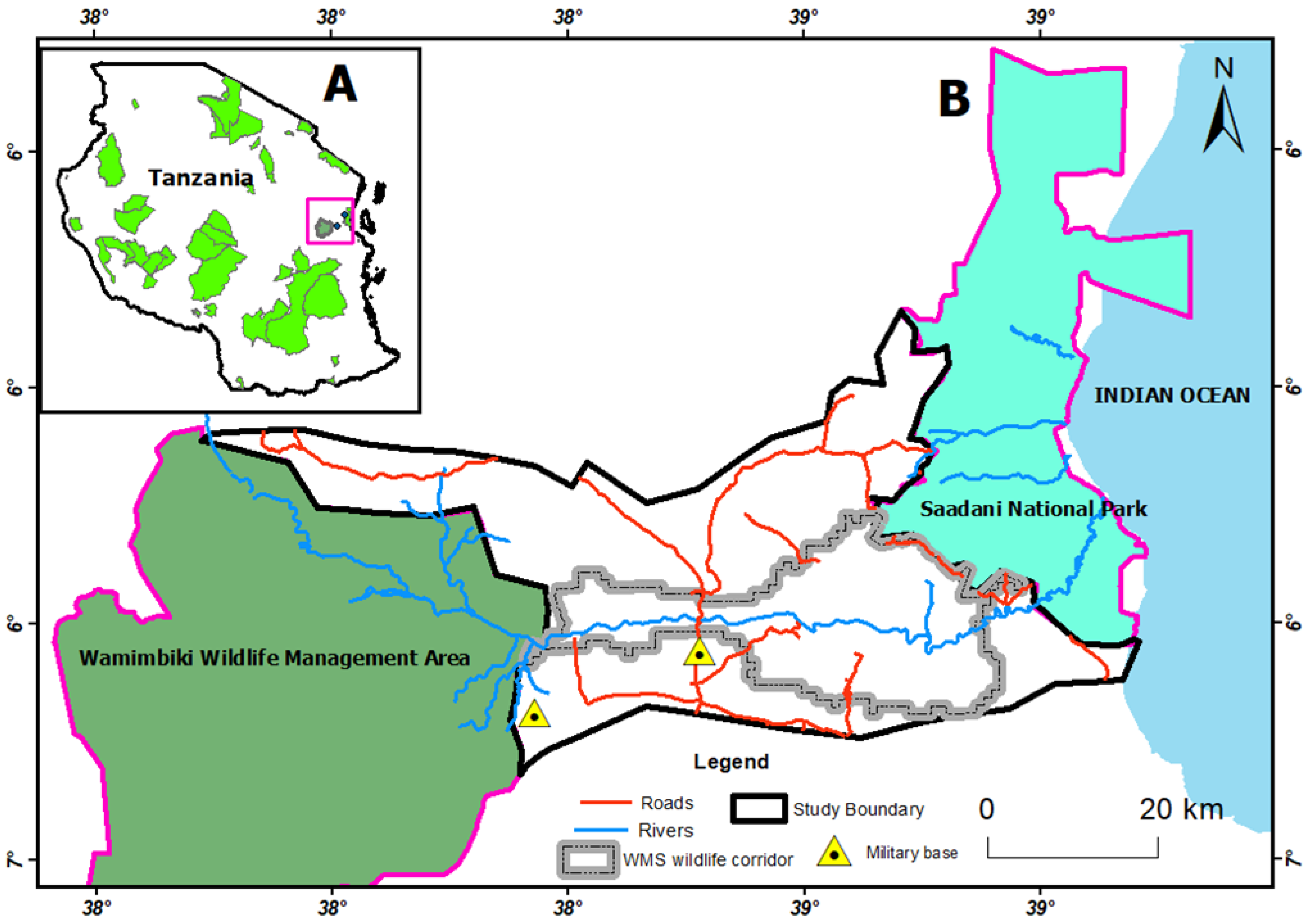
2.1. Description of the Study Area

The Wami Mbiki–Saadani (WMS) wildlife corridor is part of the Wami Mbiki–Saadani Ecosystem in Tanzania’s wildlife-rich northeastern tourist circuit [35]. The corridor in Eastern Tanzania connects Saadani National Park, Mikumi National Park, Nyerere National Park, and Selous Game Reserve via the Wami Mbiki Wildlife Management Area (WMA) as a stepping stone to offer a refuge for migratory wildlife as they travel from one protected area to another [32]. The approximately 2063 km2 large area (5°0′40″ and 6°0′40″ S, 37°50′0″and 38°50′0″ E) spans an altitudinal gradient of approximately 875 m above sea level [36]. The Wami River sub-basin is a unique ecosystem linking terrestrial and marine ecosystems [32,36,37]. The WMS wildlife corridor lies within this region and in one of the world’s known hotspots of biological diversity. It includes both the Eastern Arc Mountains and coastal forest [36] (Figure 1), with the Wami River flowing east through the center of the Wami Mbiki wildlife management area toward the southern tip of Saadani National Park [38]. The climate is warm, with a mean daily temperature of 25 °C and mean annual rainfall of over 1000 mm [36,39], with dry periods occurring from July to October and wet periods from November to December and from March to June [36]. The WMS wildlife corridor is essential in Tanzania [23], and the African elephant is one of the iconic large mammal species that use the corridor. The corridor was classified as being under extreme threat of disappearance in the imminent future if no intervention is performed for its protection [23]. The vegetation type is lowland and coastal forest, with scattered patches of miombo woodlands in some parts of the ecosystem [38]. The area comprises a complex mosaic of land cover interspersed with human settlements; pastoralists; small shifting cultivation agriculturalists; large-scale agriculture, especially sugar plantations in the eastern part of the corridor; and infrastructure development, which poses significant challenges for wildlife conservation in Eastern Tanzania.

2.2. Data Collection

2.2.1. Remote-Sensing Image Classification

In consideration of seasonality, cloud cover and phenological effects, we selected dry season remote sensing images with a minimum cloud cover of <10% and were downloaded from Earth Explorer (https://earthexplorer.usgs.gov) web plat form (accessed on 15 January 2020) for image processing and change analysis. We used satellite images (Landsat 7 ETM and Landsat 8) from 1998, 2008, and 2018 for land-use/land-cover (LULC) change classifications, downloaded via Google Earth Code Editor [40,41]. We conducted visual and digital image preprocessing before images were extracted from the full scenes as subset scenes. We used the UTM coordinate zone 37 South and prepared a color composite band (4,5,3), with its contrast being stretched by a standard deviation to enhance visual interpretability of vector features, such as rivers, agricultural land, forests, etc. The image processing was conducted by using ArcGIS software version 10.8.
We used Maximum Likelihood Classifier (MLC) for supervised image classification and to create a base map, as it considered the spectral variation within each category and the cover overlap of the different classes and was verified on the ground. Accordingly, land use and land cover were classified into seven classes: forest, bushland, agriculture with scattered settlements, grassland, bare soil, water, and urban area (Table 1). Random Forest (RF) classification using RF classifier in R generated the final land-use/land-cover map [42]. We then filtered the classified images by using a majority-neighborhoods’ filter to eliminate smaller patches and replaced them with the most common value among the neighboring pixels.

2.2.2. Analyzing Land-Cover Change

We used a post-classification comparison to quantify the extent of land-use/land-cover changes over 20 years (1998, 2008, and 2018) for high change-detection accuracy and to validate remotely sensed data by comparing classified images with the provided ground-truth data [44]. We performed an accuracy assessment based on ground-truth data collected in the field, together with high-resolution images from Google Earth, and executed a cross-tabulation between the class values and reference data, and we presented the results as an error matrix. We also performed a non-parametric kappa test to measure the extent of accuracy of classification and presented the results in confusion matric. In addition, we used the spatial analyst tool in Arc GIS to calculate change detection matrix tables for 1998–2008 and 2008–2018 and plotted the land-cover conversion to other classes. Estimation for the rate of change for different land use/land cover was computed based on the following formulae [45]:
%   C o v e r   c h a n g e = A r e a i y e a r   x A r e a i y e a r x + 1 i = 1 n A r e a i y e a r   x × 100  
A n n u a l   r a t e   o f   c h a n g e = A r e a i   y e a r   x A r e a i   y e a r   x + 1   t y e a r s
%   A n n u a l   r a t e   o f   c h a n g e = A r e a i   y e a r   x A r e a i   y e a r   x + 1   A r e a i y e a r x × t y e a r s × 100
where Area iyearx = area of cover i at the first date, Areaiyearx+1 = area of cover i at the second date, i = 1 n A r e a   i y e a r x is the total cover area at the first date, tyears = period in years between the first and the second scene acquisition.

2.3. Human–Elephant Conflicts (HEC)

Data on human–elephant conflicts (HEC) in the WMS wildlife corridor were obtained from reports collected by the District Game Officer’s office of Bagamoyo, Chalinze, and Handeni District councils and the Tanzania Wildlife Research Institute (TAWIRI). The reports comprised the complaints of villagers whose crops had been raided or who have been injured or their livestock impacted by wildlife, spanning the years 2016 to 2020. The reports indicated the location, type, and extent of destroyed crops; and the livestock species and numbers affected/killed by elephants, as well as human killings or injuries by elephants. Each incident was classified as a unique event. In addition, we computed and mapped the distances of HEC locations to the park boundaries, to the nearest road, and nearest river by using ArcGIS software. A Kernel Density Estimation (KDE) and Gedis-Ord Gi algorithms were carried out to identify high concentration and hotspot areas of HEC. We combined the KDE surface with different LULC classes and generated a HEC hotspot risk map. According to time of records, the spatiotemporal distribution points collected by HEC reports across different locations were overlaid with the land-use/land-cover map according to time of records to reveal the preferred habitat for the elephants in the WMS corridor.

2.4. Habitat Suitability Modeling

For the habitat suitability model for the WMS wildlife corridor, we used the elephant as model species for the span of two decadal time steps (1998, 2008, and 2018). For habitat suitability modeling, it is most important to identify factors that influence the spatial distribution of animal species to develop effective conservation planning and habitat suitability evaluation [46]. We selected these factors based on the elephant-distribution literature [24,35,46,47,48], as well as the locations of HEC through reports across the entire WMS corridor. We included four key environmental variables as basic representative criteria of main features of suitable habitat for elephants [24]: land-cover structure (vegetation cover), proximity to permanent water, Normalized Difference Vegetation Index (NDVI), and proximity to road networks [49,50,51,52] (Table 2). Elephants tend to rest in shaded areas during the day when not moving [48,53,54], and areas with high tree cover can act as refuge in areas of high human activity [55] and provide foraging areas. We, thus, classed forest as optimal habitat, and the more forest patches, the better the habitat. Each factor was assigned a value based on the Analytical Hierarchy Process (AHP) [56]. The AHP is the most used multi-criteria decision-making method to determine weightage for assigning, in particular, habitat parameters [47,57]. The AHP assumed that some factors are more important than others for the species under study [58].
The Analytical Hierarchy Process (AHP).
The AHP is a flexible and structured GIS-based model for analyzing and solving complex decision-problems work [56] to rank and select the best in a set of alternatives. The ranking is performed concerning an overall goal and broken down into criteria (objectives and attributes), applying a nine-point scale of measurements: 1 = equal importance, 3 = moderate importance, 5 = strong importance, 7 = very strong importance, and 9 = extreme importance. The intermediate values 2, 4, 6, and 8 help grading between two adjacent judgments [59]. The AHP method was selected because we did not have many species location data available and AHP allows habitat modeling when empirical data are scarce [51,52]. For our AHP model, the main factors for the elephant habitat suitability were land-use/land-cover change, NDVI, proximity to permanent water, and proximity to road. The alternatives or sub-factors were bushland, agriculture, forest, grassland, and urban area. Each criterion was given a value according to Reference [56] (Table 2).
We conducted a pairwise comparison (Table 3a) to reduce the conceptual complexity, since only two components were considered at any given time, developing a comparison matrix, computing and assigning weights for each element in the hierarchy tree, and normalizing those to determine the priority vector (Eigen vector) (Table 3b). The associated rank weight (AR) values were used in estimating the consistency ratio (C/R). The priority vector, also known as the normalized principal Eigen vector, was calculated by determining the means of the rows of the normalization table (Table 3).
Estimation of the consistency ratio (CR).
The following formula computed the consistency ratio (CR) [56]. The CR is used to confirm that the matrix judgements were randomly generated [56,58].
C R = C I R I
where CI is the consistency index, RI is the random consistency index, and CR is the consistency ratio.
C I = λ m a x n n 1
where λmax is the principal Eigen value, i.e., the sum or the products between each element of the priority vector and column totals; n is number of factors; and the random consistency index = 0.9 for four factors, CI = 4.3 [56,58]. After computing the CR, potential parameters were integrated in the GIS domain [2,60] to determine the elephants’ different levels of habitat suitability. First, vector layers (proximity to permanent water and road distance) were converted into raster format and multiplied with their specific weight. Next, we conducted kernel density estimation to generate raster-based maps from vector data (river shape files) and human disturbances (land use and road networks) in Arc GIS 10.8. Afterward, the resulting raster layer values were combined to get the final habitat suitability map. We used the weight analysis method in the novel habitat suitability model to extract the suitable habitat area based on Equation (6). Here, the suitable habitat area (SHA) was computed in the weighted overlay tool in ARC GIS as follows:
S H A = [ ( L U L C w i ) + ( P w w i ) + ( P r w i ) + ( N D V I w i ) ]
where LULC is land use/land cover, Pw is proximity to permanent water, Pr is proximity to road networks, and NDVI is the Normalized Difference Vegetation Index. The subscript wi is the weights of individual habitat suitability factors.

2.5. Habitat Fragmentation Analysis

We conducted landscape habitat fragmentation analysis to designate the spatial configuration of landscape metric classes of interest [61], using Fragstat 4.2 landscape metrics [3,62,63]. Landscape metrics are a quantitative link between landscape patterns and ecological or environmental processes [64]. They display numerical information about landscape composition, configuration, and dimensions; allow for comparisons of different times; and even help recreate future scenarios [65]. They have become useful in linking patterns found in the landscape to various environmental and ecological processes [64]. We calculated class and landscape-level statistics for raster GeoTIFF land-use/land-cover classes of 1998, 2008, and 2018. We calculated landscape metrics for class levels, such as the total class area (CA), percentage of landscape (PLAND), edge density (ED), patch density (PD), number of patches (PN), landscape shape index (LSI), interspersion and jurisdiction index (IJI), and largest patch index (LPI) [66]. In addition, we calculated Shannon’s Diversity Index (SHDI) for landscape-level metrics (Table 4), as rare patch types have a considerable influence on the extent of the index [67]. LSI enables us to measure a standardized total edge, while ED adjusts for the size of the landscape; LPI at the class level quantifies the percentage of total landscape area comprising the largest patch; it is a measure of dominance [68]. Specifically, NP is an outstanding measure of the fragmentation of a given class within the landscape, since the landscape size is continuous. IJI provides metrics of shape and interspersion.

2.6. Statistical Analysis

To avoid multi-collinearity, we created a Pearson’s correlation matrix for all landscape structure metrics and removed ED and LSI (|r|) ≥ 0.60, because they showed a high correlation with several other variables. Using Principal Component Analysis (PCA), we examined the variance structure among the remaining conformation metrics to ordinate and reduce superfluous variables. PCA based on the correlation metrics with varimax rotation revealed the differences in multivariate space. Biplot diagrams showed the correlation structure of the variables, besides indicating the changes based on the involved metrics [2]. These components explained 89.2% of the cumulative proportion of variance. We observed the highest loading scores among PLAND, LPI, IJI, PD, NP, and CA and selected these landscapes metrics for further analysis. These metrics were chosen and used because they have been robust and efficient for characterizing the land-cover fragmentation at the land-cover-class level. We conducted a post hoc analysis based on Turkey’s to see significant changes in landscape metrics across different land-use classes and years of investigation; the results are presented in Supplementary Materials Tables S1–S6. The statistical analyses were performed by using R software [69] and the factor Miner package [70].

3. Results

3.1. Accuracy Assessment

The overall accuracy assessment for LULC change classification levels for the three-time step ranges from 75% to 97%, with kappa agreement indices ranging from 0.71 to 0.75. Accuracies per individual LULC classes, i.e., user’s accuracy (UA) and producer’s accuracy (PA), are presented in Table 5. The values for the three classification results are satisfactory for the study area because they satisfy a minimum of 71%, which agrees with the [71] classification scheme. According to Reference [72], the kappa agreement is poor when k < 0.4, good when 0.4 < k < 0.7, and excellent when k > 0.75. Thus, according to these agreement schemes, our classification denotes good-to-excellent agreement. The overall accuracy of our study is considered acceptable based on Reference [71]. The results provide a major platform for the subsequent analysis of LULC changes.

3.2. Land-Use/Cover Change in the WMS Wildlife Corridor over the Last 20 Years

We created two transition matrices in land cover for 1998–2008 and 2008–2018, analyzing change detection by cross-tabulation and plotted graphs for land-cover conversions to other cover classes. The results revealed that there were significant changes in land use/land cover between the time of investigation. Over the past two decades, the WMS wildlife corridor has witnessed a large forest cover loss (Table 6), whereby between 1998 and 2008, forest cover declined by 3.1% and further by 20.3% between 2008 and 2018. In contrast, agriculture and grassland increased, while bushland declined from 34.0% in 1998 to 25.2% in 2018. In 1998, forest area occupied 55.0%, followed by bushland with 34.0% (Table 6).
The urban settlement area increased only slightly by 0.1% between 1998 and 2018 (Table 6). The forest showed a high annual rate of change from 6.4 km2/year between 1998 and 2008 to 41.6 km2/year in 2008–2018 (Table 6). The overall urban-area-cover class is small compared to other land-use/cover classes but significant in wildlife habitat conservation, as all urban centers were located within the wildlife corridor. The road network expanded more than twice as much to approximately 500 km in 2018 compared to 216 km in 1998. The length of secondary roads increased only slightly from 79 km in 1998 to 98 km in 2018.

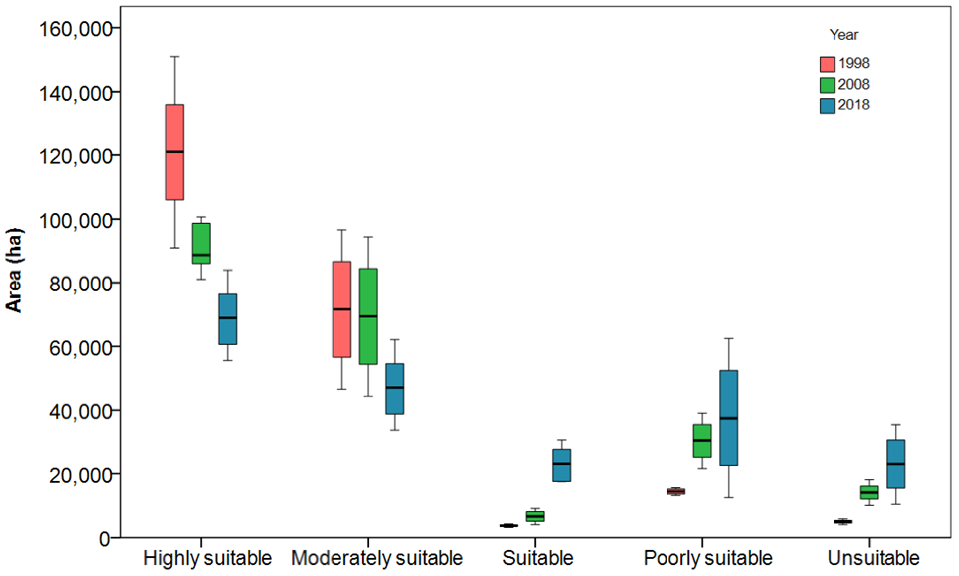
3.3. Habitat Suitability Change for Elephants

Our AHP model revealed that LULC (45.6%), proximity to permanent water (29.8%), vegetation status (NDVI) (22.0%), and proximity to road (2.5%) were the most influential habitat suitability parameters for elephants (Table 3). The Consistency Ratio (CR) computed through AHP was 4.8%, which is within the accepted range but lower than the reasonable level of acceptance (<10%) [56]. The highly suitable habitat areas decreased in total by 22.4% between 1998 and 2018 (Figure 2). The unsuitable habitat (Category 1) increased only slightly by 3.8% between 1998 and 2008 and by 0.2% between 2008 and 2018 (Figure 2). Moderately suitable habitat decreased by 1.4% between 1998 and 2008 and again declined by 6.5% between 2008 and 2018, while poorly suitable habitat increased by 2.8% between 1998 and 2008 and by 21.2% between 2008 and 2018. Suitable habitat area rose by 0.6% between 1998 and by 8.1% between 2008 and 2018, especially in areas near Saadani National Park. Forest patches significantly declined over time (Figure 2), and this has also led to a significant decline in areas of moderately suitable and highly suitable habitat.

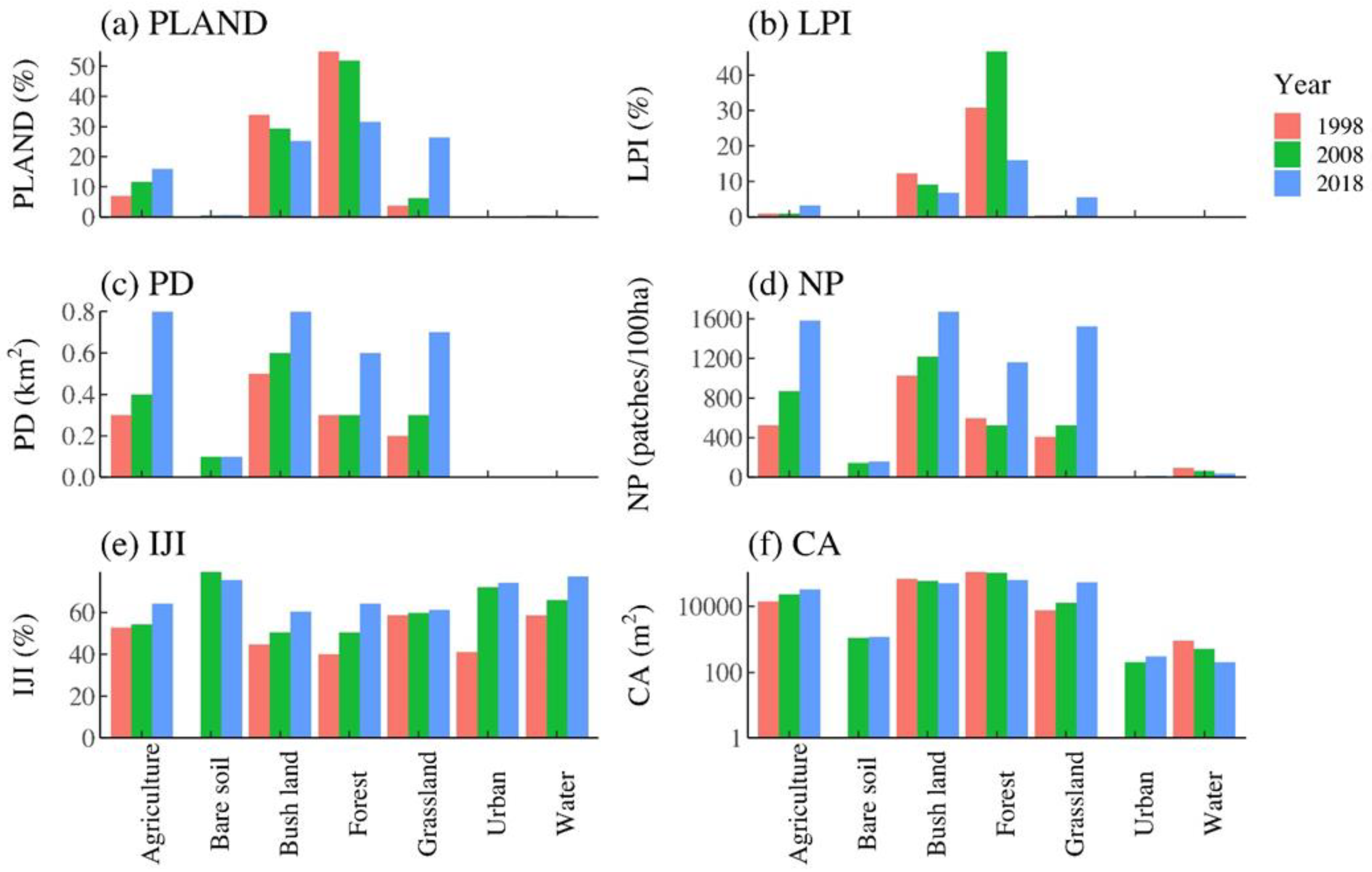
3.4. Landscape Metrics Analysis

Our results showed that the forest comprised the highest percentage of the landscape (PLAND) compared to other habitat types over the entire period and decreased from 55.0% in 1998 to 51.0% in 2008 and further to 16.0% in 2018 (Figure 3a and Supplementary Table S4). The forest’s largest patch index (LPI) for bushland decreased by 27.0% between 1998 and 2008 and 1.2% between 2008 and 2018 (Figure 3b), highlighting that the landscape became considerably fragmented between 1998 and 2018 in the WMS wildlife corridor. The Shannon’s Diversity Index (SHDI) of the landscape metrics increased from 1.0 in 1998 to 1.2 in 2008 and then to 1.4 in 2018, further indicating an increase in landscape fragmentation in the WMS wildlife corridor [73]. PLAND significantly increased for bushland (21.8%, p < 0.001) and agriculture with scattered settlements (29.4%, p < 0.001), while it declined for forest area (29.0%, p < 0.001; Supplementary Table S1). The same trend was observed for forests compared to bushland and grassland (Supplementary Table S2). The increase in PD and NP (Supplementary Tables S4 and S5) and decrease in LPI over time, especially for the bushland class, indicates significant landscape fragmentation due to the cohesion of bushland [74]. IJI shows some increasing trends, but there was no significant difference (Figure 3e and Supplementary Table S6), suggesting that patches are not well-interspersed or equal to other patch types. The CA for bushland and forest (Figure 3f) decreased from 69,742 and 113,074 ha in 1998 to 65,036 and 32,900 ha in 2018, respectively, indicating high conversion of bushland and forest land into agricultural land and other land uses. We also conducted a multivariate analysis, using PCA on landscape metrics based on Root Mean Square Root Residual, off diagonal (RMSR) and Goodness of Fit Index (GFI) values [2]. The model explained 89.2% of the total variance. PC1 explained 67.0% and PC2 22.2% of the variance based on the PCA, with individual variable contributions shown in Appendix A Figure A1.

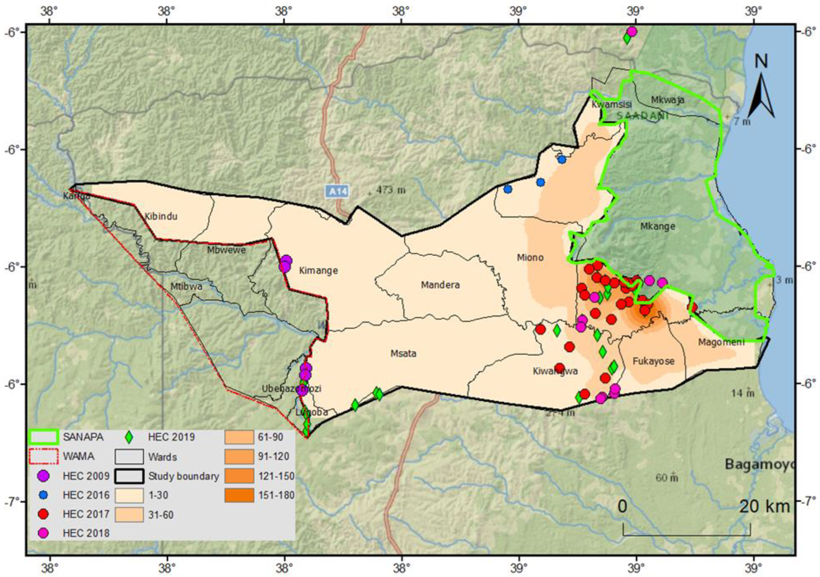
3.5. Human–Elephant Conflict and Hotspot Locations

In total, 621 HEC incidences were collected from Handeni, Chalinze, and Bagamoyo District Councils between 2016 and 2020, with the highest incidences recorded in 2017 (N = 290) and the lowest in 2020 (N = 16). The HEC frequencies decreased with increasing distance from the protected area into the corridor, corresponding to elephants’ unsuitable and poorly suitable habitat. HEC incidences were reported more often in the wet season (N = 569), i.e., between November and February, than in the dry season (N = 52; Figure 4. The most frequently reported HEC was crop-raiding (73%), while human and livestock injuries comprised 23% of the cases. The most strongly affected villages were about 3 to 5 km away from protected areas, including Gongo, Kiwangwa, Matipwili, and Kwangandu (Figure 4). Crop-raided agricultural areas had increased dramatically from 300 ha in 2017 to 426 ha in 2019.

4. Discussion

4.1. Forest Loss and Agricultural Expansion in the Corridor

Our results showed that urban areas, grassland, and agriculture with scattered settlements have expanded in the Wami Mbiki–Saadani wildlife corridor over the last 20 years, while forest and bushland have strongly declined. Likely, these changes have been caused by a rapid human population growth [75,76], agricultural expansion, infrastructure development, and forest clearance for timber and charcoal production. Over time, the decline in water might have been caused by the destruction of riverbanks, which led to high surface runoff during the rainy season followed by drying of rivers, especially the tributaries of the Wami river [77,78]. Our results identified the locations of different socio-economic activities that acted as the driving forces for land-cover changes in the WMS Saadani wildlife corridor. These activities could be attributed to an increasing human population growth; that is, the number of people living in the corridor increased from 311,627 in 2002–2012 to 356,320 in 2018, according to Reference [79]. Population increases have been caused by the immigration of people from different parts of the country seeking fertile land for agriculture, especially for pineapple growing, grazing pastures, and charcoal burning [9]. In addition, the poverty of local communities along the corridor was identified as one important reason for enhancing shifting cultivation practices [9]. These activities have caused the decline in forest cover in WMS which is a well-known phenomenon in other parts of the world, where forest loses are often caused by increased human populations and, consequently, declines in biodiversity [80,81].
Our LULC analyses highlighted the vulnerability, degradation, and loss of wildlife habitats, which will negatively affect biodiversity conservation [82]. A destruction of elephant habitat (i.e., forest) and foraging areas and an interruption of elephant movement might lead to large-scale blockage of the entire WMS corridor, which was already mentioned as a possible scenario by AHP. Reference [83] reported that overgrazing, shifting cultivation, and charcoal burning were significant factors for the degradation of the wildlife corridors in Njombe and Mbalizi districts, Tanzania, as was also observed by Reference [23].
Our results showed that although the WMS wildlife corridor forms an important connection between the Saadani National Park and Wami Mbiki Wildlife Management Area [84], its status has been decreasing with time, particularly the cover and connectivity of natural vegetation. We, thus, highlight that the WMS wildlife corridor comprises a fragile ecosystem of lowland and coastal forests, where agricultural activities are becoming increasingly common, which needs particular attention for protection to guarantee human–wildlife coexistence.

4.2. Habitat Suitability and Quality Decline over Time

Our results from AHP indicated that the forest and bush cover were the most influencing parameter in the distribution of elephant habitat in the study area, which is consistent with other studies [24,46,47], as the elephants are undisturbed and can acquire food in such types of habitat. We found that the highly and moderately suitable habitats for elephants decreased by 22.4% and 8.1% within the WMS ecosystem, especially in the wildlife corridor, respectively, over the last 20 years. In 1998, the highly suitable habitat (57.6%) dominated the southwestern part of the corridor, near the Wami Mbiki WMA. Likely, as protection and conservation activities by the Wami Mbiki society have been rather intense, it received conservation funds for conservation activities, such as regular patrol, from a tourist hunting company until the late 2010s [30,84]. However, more poorly suitable and unsuitable habitats became visible in the northeastern and middle parts of the WMS corridor, in the later years, likely due to the intensification of agricultural activities around urban areas. A slight increase in suitable habitat on the northeastern part might have been due to upgrading the former Mkwaja ranch to Saadani National Park and improving mangrove protection within Saadani National Park (SANAPA), [84], as well as due to the establishment of the Kisampa conservancy adjacent to Saadani National Park, which is a private community conservation sanctuary covering 60 km2, established in 2004, Kisampa Conservancy (http://www.afrikaafrikasafaris.com/kisampa-overview/) web page accessed on 25th January 2020.
In contrast, the unprotected areas in the corridor exhibited poor and unsuitable habitats. Furthermore, the intensification of infrastructure, such as roads and construction of two military bases at Wami and Pongwe Kwa Msungura, which are within the wildlife corridor, likely stipulated settlements and agricultural activities, thereby restricting elephant migration routes [85]. A hampered migration might foster genetic isolation of wildlife in the near future [86,87,88,89], since connectivity between the protected areas will be hampered [90,91,92,93,94,95]. As we used the elephant as an umbrella species, whose protection can facilitate the linkage, i.e., corridor networks, for multiple other wildlife species [96], our results showed that the highly and moderately suitable habitat likely also declined for other wildlife species, thus signifying an urgent need for habitat restoration of the WMS corridor.

4.3. Elephant Distributions and HEC Hotspots

The results from human–elephant conflict (HEC) reports showed the distributions of HECs close to the protected areas, especially Saadani National Park, which might be due to habitat loss and corridor blockage by human activities, limiting wildlife movements [29,32,97]. This might also have caused the increase in human–elephant conflicts in our study area, as people encroached on the wildlife corridor, restricting mammal movement close to protected areas (PAs), a phenomenon also found in other areas of Tanzania and other parts of the world [98,99]. The high HEC occurrences within 3–5 km away from the protected areas is in agreement with Harich [100], who showed that Asian elephants (Elephas maximus indicus) only moved less than 3 km away from protected areas into cultivated land, i.e., rubber plantations, in Thailand.

4.4. Overall Landscape Fragmentation in WMS Wildlife Corridor

Our landscape metrics analysis showed that PLAND was highest for forest compared to other habitat types over the entire period but declined rapidly over time, thus highlighting the dominant processes of landscape fragmentation [63] in our study area. References [101,102] have shown a strong relationship between landscape fragmentation and wildlife habitat loss. The largest patch index (LPI) changes indicated that wooded patches have drastically declined in size and connectivity, as was also seen for forests in the Lincang River Valley of China [103], leading to a general decline in wildlife biodiversity [103,104]. Generally, a declining LPI leads to habitat exposure to edge effects, which are often associated with loss in biodiversity through the loss of habitat area [105,106].
In our study, we only had limited information on elephant distribution data and used a rather coarse land-cover-classification scheme. However, our land-use metrics model, in combination with LULC changes, as well as HEC conflict data, highlighted areas of conservation importance within the corridor. We showed that deriving habitat indices for mega herbivores can help drawing attention to rapid declines in habitat availability, illustrate hotspot areas of decline, and, thus, point out areas of concern for managers.

5. Conclusions

Our study on land-cover change and landscape fragmentation has revealed severely impacted elephant habitat in the Wami Mbiki–Saadani wildlife corridor within the last two decades. Our combination of LULC change maps and habitat suitability features with conflict abundance data stressed a constant decrease in highly suitable habitat for elephants. The wildlife corridor experienced a strong forest decline and agriculture expansion, and the landscape has become more fragmented for elephants.
Our findings highlight an urgent need to strengthen the conservation of significant wildlife habitat through community conservation awareness and extension programs, which advocate the sustainable utilization of natural resources. We suggest conducting aerial surveys in addition to our study, especially in the wildlife corridor, to see the levels of habitat loss and whether the corridor is still accessible and used by wildlife. We pinpoint spatial and temporal trends of HEC occurrences and relate those to large-scale landscape matrix properties in the WMS wildlife corridor. We further stress the negative impacts of human activities on elephant habitat and suggest that management should promote human–wildlife coexistence in this fragile ecosystem. We recommend that communities living within or adjacent to wildlife corridors plant crops less preferred by elephants or use prevention measures, to enable human–elephant coexistence in the Wami Mbiki–Saadani ecosystem.

6. Implication for Conservation

Our study combined remote sensing and GIS, as well as secondary data and landscape metrics quantifications, for modeling habitat suitability for elephants. This can be useful and essential for helping to provide timely and accurate data for modeling and mapping habitat suitability for elephants. We further show how HEC data can be used to derive heat maps and indicate hotspot areas, where mitigation and prevention of conflicts can be focused on. Our work showed general trends of wildlife conservation challenges, such as the decline of the African elephant habitat due to increasing anthropogenic activities, especially outside protected areas, which can be applied in various ecoregions [39,74,95]. Our study revealed a decreasing area of highly and moderately suitable habitat and an increase of unsuitable and poorly suitable habitats over time. We conclude that the WMS corridor is highly threatened and claim that essential environmental variables, such as vegetation cover, NDVI status, LULC change, and water sources, should be prioritized for habitat suitability models, while planning the wildlife corridor management strategies.
Our ranking of the habitat suitability parameters computed by AHP can be used as a general guideline to identify optimal elephant habitat locations [24,95]. We stress that landscape analysis knowledge is essential for keystone species conservation, such as the African elephant, whose population is declining across a range of unprotected and protected areas [107].

Supplementary Materials

The following are available online at https://0-www-mdpi-com.brum.beds.ac.uk/article/10.3390/land11020307/s1, Table S1: The mean (%) difference (Tukey Post–Hoc Test) for landscape fragmentation for PLAND among land use, Table S2: The mean (%) difference (Tukey Post–Hoc Test) for landscape fragmentation for LPI among land use, Table S3: The mean (Ha) difference (Tukey Post–Hoc Test) for landscape fragmentation for CA among land use, Table S4:The mean (Km2) difference (Tukey Post–Hoc Test) for landscape fragmentation for PD among la Table S5: The mean difference (Tukey Post–Hoc Test) for landscape fragmentation for NP among land use nd use, Table S6: The mean (%) difference (Tukey Post–Hoc Test) for landscape fragmentation for IJI among land use.

Author Contributions

L.T.N., conceptualization, methodology, software, formal data analysis, data curation, writing initial draft preparation, and project administration; L.K.M. and A.C.T., methodology, validation, and interpretation of results; E.K., data contribution; A.C.T., E.K. and L.K.M., reviewing and editing of the manuscript. All authors have read and agreed to the published version of the manuscript.

Funding

This research received funding from CREATES grant number BG.129/649/04/75. The APC will be funded from individual sources.

Institutional Review Board Statement

Not applicable.

Informed Consent Statement

Not applicable.

Data Availability Statement

Not applicable.

Acknowledgments

Special thanks to Y.J. Magangali, who helped during data collection, and O. Simon from the Institute of Resource Assessment (IRA), University of Dar es Salaam, for technical support during land-use/land-cover classifications. This research has a clearance permit No. 2020-209-NA-2020-082 from Tanzania Commission for Science and Technology (COSTECH) and was permitted by the Tanzania Wildlife Research Institute, Tanzania National Parks, and Tanzania Wildlife Area.

Conflicts of Interest

The authors declare that there is no potential conflict of interest.

Appendix A

Table A1. Landsat images used to map land-cover classes of the Wami Mbiki–Saadani wildlife corridor in 1998, 2008, and 2018. Source: Earth Explorer (https://earthexplorer.usgs.gov) web plat form accessed on 15 January 2020. All images have <10% cloud cover.
SensorYearPath/RowResolution
Landsat TM1998167/065. 167/064. 166/064 and 166/06530 m
Landsat TM2008167/065. 167/064. 166/064. and 166/06530 m
Landsat 82018167/065. 167/064. 166/064. and 166/06530 m
Table A2. Landscape fragmentation metrics used in this study (McGarigal, 2002) are compared over the years 1998, 2008, and 2018 for the study area in WMS wildlife corridor, Tanzania. Land-cover classes according to Table 3. CA = class area, PLAND = percentage of landscape, NP = number of patches, PD = patch density, LPI = largest patch index, ED = edge density, LSI = largest shape index, IJI = interspersion and juxtaposition index.
MetricsCA (m2)PLAND (%)NP (#/100 ha)PD (km2)
Land Use199820082018199820082018199820082018199820082018
Forest113,074106,70232,90055.051.916.059752415820.30.30.8
Bushland69,74260,16465,03633.929.331.61026121811610.50.60.6
Agriculture14,34223,76954,2277.011.626.452787015240.30.40.7
Grassland758812,92851,7223.76.325.240852416740.20.30.8
Bare soil0.0112411830.00.50.601451600.00.10.1
Water8665492470.40.30.19463360.00.00.0
Urban161883070.00.10.117160.00.00.0
MetricsLPIED (m/ha)LSI (n/a)IJI (%)
Land Use199820082018199820082018199820082018199820082018
Forest30.846.73.224.625.115.839.241.045.340.050.364.2
Bushland12.39.116.025.924.424.551.452.250.544.650.564.2
Agriculture1.01.05.66.811.427.829.538.962.552.854.361.1
Grassland0.40.46.83.96.327.923.229.064.158.759.860.5
Bare soil0.00.00.00.00.80.90.012.613.20.079.475.5
Water0.00.00.00.60.40.210.28.56.158.665.877.3
Urban0.00.00.00.00.10.21.03.54.341.172.274.1
Figure A1. Variable distributions and their according contributions based on Principal Component Analysis (PCA) in Wami Mbiki–Saadani wildlife corridor, Tanzania, toward our landscape analysis. Contrib = contribution, LPI = largest patch index, CA = total class area, PLAND = percentage of landscape, PD = patch density, NP = number of patches, IJI = interspersion and juxtaposition index. The color ramp indicates the variable contribution importance to PC1 (Dim1) and PC2 (Dim2).
Land 11 00307 g0a1

References

  1. Singh, S.K.; Srivastava, P.K.; Szabó, S.; Petropoulos, G.P.; Gupta, M.; Islam, T. Landscape transform and spatial metrics for mapping spatiotemporal land cover dynamics using Earth Observation data-sets. Geocarto Int. 2017, 32, 113–127. [Google Scholar] [CrossRef] [Green Version]
  2. Kumar, M.; Denis, D.M.; Singh, S.K.; Szabó, S.; Suryavanshi, S. Landscape metrics for assessment of land cover change and fragmentation of a heterogeneous watershed. Remote Sens. Appl. Soc. Environ. 2018, 10, 224–233. [Google Scholar] [CrossRef] [Green Version]
  3. Saikia, A.; Hazarika, R.; Sahariah, D. Land-use/land-cover change and fragmentation in the Nameri Tiger Reserve, India. Geogr. Tidsskr. J. Geogr. 2013, 113, 1–10. [Google Scholar] [CrossRef]
  4. Karlson, M.; Mörtberg, U.; Balfors, B. Road ecology in environmental impact assessment. Environ. Impact Assess. Rev. 2014, 48, 10–19. [Google Scholar] [CrossRef]
  5. Jones, T.; Bamford, A.J.; Ferrol-Schulte, D.; Hieronimo, P.; McWilliam, N.; Rovero, F. Vanishing Wildlife Corridors and Options for Restoration: A Case Study from Tanzania. Trop. Conserv. Sci. 2012, 5, 463–474. [Google Scholar] [CrossRef]
  6. Hefty, K.L.; Koprowski, J.L. Multiscale effects of habitat loss and degradation on occurrence and landscape connectivity of a threatened subspecies. Conserv. Sci. Pract. 2021, 3, e547. [Google Scholar] [CrossRef]
  7. Serieys, L.E.K.; Rogan, M.S.; Matsushima, S.S.; Wilmers, C.C. Road-crossings, vegetative cover, land use and poisons interact to influence corridor effectiveness. Biol. Conserv. 2021, 253, 108930. [Google Scholar] [CrossRef]
  8. Thatte, P.; Joshi, A.; Vaidyanathan, S.; Landguth, E.; Ramakrishnan, U. Maintaining tiger connectivity and minimizing extinction into the next century: Insights from landscape genetics and spatially-explicit simulations. Biol. Conserv. 2018, 218, 181–191. [Google Scholar] [CrossRef]
  9. Ebenezeri Kileo, L.; Emmanuel Mbije, N. Land Use Practices along Saadani-Wami-Mbiki Wildlife Corridor and their Implications to Wildlife Conservation. Asian J. Environ. Ecol. 2021, 16, 126–143. [Google Scholar] [CrossRef]
  10. Ghent, C. Mitigating the effects of transport infrastructure development on ecosystems. Consilience 2018, 19, 58–68. [Google Scholar]
  11. Erena, M.G.; Yesus, T.G. Mapping potential wildlife habitats around Haro Abba Diko controlled hunting area, Western Ethiopia. Ecol. Evol. 2021, 11, 11282–11294. [Google Scholar] [CrossRef] [PubMed]
  12. Taylor, A.C.; Walker, F.M.; Goldingay, R.L.; Ball, T.; Van Der Ree, R. Degree of landscape fragmentation influences genetic isolation among populations of a Gliding mammal. PLoS ONE 2011, 6, e26651. [Google Scholar] [CrossRef] [PubMed]
  13. Brashares, J.S.; Arcese, P.; Sam, M. Human demography and reserve size predict wildlife extinction in West Africa. Biol. Sci. 2001, 268, 2473–2478. [Google Scholar] [CrossRef] [PubMed] [Green Version]
  14. Craigie, I.D.; Baillie, J.E.M.; Balmford, A.; Carbone, C.; Collen, B.; Green, R.E.; Hutton, J.M. Large mammal population declines in Africa’s protected areas. Biol. Conserv. 2010, 143, 2221–2228. [Google Scholar] [CrossRef]
  15. Ogutu, J.O.; Piepho, H.-P.; Said, M.Y.; Ojwang, G.O.; Njino, L.W.; Kifugo, S.C.; Wargute, P.W. Extreme wildlife declines and concurrent increase in livestock numbers in Kenya: What are the causes? PLoS ONE 2016, 11, e0163249. [Google Scholar] [CrossRef]
  16. Van Eeden, L.M.; Eklund, A.; Miller, J.R.B.; López-Bao, J.V.; Chapron, G.; Cejtin, M.R.; Crowther, M.S.; Dickman, C.R.; Frank, J.; Krofel, M. Carnivore conservation needs evidence-based livestock protection. PLoS Biol. 2018, 16, e2005577. [Google Scholar] [CrossRef]
  17. Bolger, D.T.; Newmark, W.D.; Morrison, T.A.; Doak, D.F. The need for integrative approaches to understand and conserve migratory ungulates. Ecol. Lett. 2008, 11, 63–77. [Google Scholar] [CrossRef]
  18. Kinnaird, M.F.; O’brien, T.G. Effects of private-land use, livestock management, and human tolerance on diversity, distribution, and abundance of large African mammals. Conserv. Biol. 2012, 26, 1026–1039. [Google Scholar] [CrossRef]
  19. Schüßler, D.; Lee, P.C.; Stadtmann, R. Analyzing land use change to identify migration corridors of African elephants (Loxodonta africana) in the Kenyan-Tanzanian borderlands. Landsc. Ecol. 2018, 33, 2121–2136. [Google Scholar] [CrossRef]
  20. Newmark, W.D. Isolation of African protected areas. Front. Ecol. Environ. 2008, 6, 321–328. [Google Scholar] [CrossRef]
  21. Shauri, V.; Hitchcock, L. Wildlife Corridors and Buffer Zones in Tanzania; LEAT: Dar Es Salaam, Tanzania, 1999; Volume 7, pp. 583–596. [Google Scholar] [CrossRef]
  22. Kideghesho, J.R. The Elephant Poaching Crisis in Tanzania: A Need to Reverse the Trend and the Way Forward. Trop. Conserv. Sci. 2016, 9, 369–388. [Google Scholar] [CrossRef]
  23. Caro, T.; Jones, T.; Davenport, T.R.B. Realities of documenting wildlife corridors in tropical countries. Biol. Conserv. 2009, 142, 2807–2811. [Google Scholar] [CrossRef]
  24. Aini, S.; Sood, A.M.; Saaban, S. Analysing elephant habitat parameters using GIS, remote sensing and analytic hierarchy process in peninsular Malaysia. Pertanika J. Sci. Technol. 2015, 23, 37–50. [Google Scholar]
  25. Naha, D.; Dash, S.K.; Chettri, A.; Roy, A.; Sathyakumar, S. Elephants in the neighborhood: Patterns of crop-raiding by Asian elephants within a fragmented landscape of Eastern India. PeerJ 2020, 8, e9399. [Google Scholar] [CrossRef]
  26. Kushwaha, C.P.; Tripathi, S.K.; Singh, K.P. Tree specific traits affect flowering time in Indian dry tropical forest. Plant Ecol. 2011, 212, 985–998. [Google Scholar] [CrossRef]
  27. Martinuzzi, S.; Vierling, L.A.; Gould, W.A.; Falkowski, M.J.; Evans, J.S.; Hudak, A.T.; Vierling, K.T. Mapping snags and understory shrubs for a LiDAR-based assessment of wildlife habitat suitability. Remote Sens. Environ. 2009, 113, 2533–2546. [Google Scholar] [CrossRef] [Green Version]
  28. Acevedo, P.; Farfán, M.Á.; Márquez, A.L.; Delibes-Mateos, M.; Real, R.; Vargas, J.M. Past, present and future of wild ungulates in relation to changes in land use. Landsc. Ecol. 2011, 26, 19–31. [Google Scholar] [CrossRef]
  29. Beca, G.; Vancine, M.H.; Carvalho, C.S.; Pedrosa, F.; Alves, R.S.C.; Buscariol, D.; Peres, C.A.; Ribeiro, M.C.; Galetti, M. High mammal species turnover in forest patches immersed in biofuel plantations. Biol. Conserv. 2017, 210, 352–359. [Google Scholar] [CrossRef] [Green Version]
  30. Gayo, L. Contribution of Wildilife Management Area on Wildlife Conservation and Livelihood: A Case of Wami-Mbiki Wildlife Management Area. Ph.D. Thesis, The University of Dodoma, Dodoma, Tanzania, 2013. [Google Scholar]
  31. Mutaka, M.M. Examining Conservation Conflicts in Tanzania’s National Parks: A Case Study of Saadani National Park. Ph.D. Thesis, Ghent University, Faculty of Political and Social Science, Ghent, Belgium, 2016. [Google Scholar]
  32. Riggio, J.; Mbwilo, F.; Van de Perre, F.; Caro, T. The forgotten link between northern and southern Tanzania. Afr. J. Ecol. 2018, 56, 1012–1016. [Google Scholar] [CrossRef]
  33. Beale, C.M.; Hauenstein, S.; Mduma, S.; Frederick, H.; Jones, T.; Bracebridge, C.; Maliti, H.; Kija, H.; Kohi, E.M. Spatial analysis of aerial survey data reveals correlates of elephant carcasses within a heavily poached ecosystem. Biol. Conserv. 2018, 218, 258–267. [Google Scholar] [CrossRef]
  34. Mariki, S.B. Successes, threats, and factors influencing the performance of a community-based wildlife management approach: The case of Wami Mbiki WMA, Tanzania. In Wildlife Management-Failures, Successes and Prospects; IntechOpen: London, UK, 2018. [Google Scholar]
  35. Debonnet, G.; Nindi, S. Technical Study on Land Use and Tenure Options and Status of Wildlife Corridors in Tanzania: An Input to the Preparation of Corridor; USAID: Washington, DC, USA, 2017.
  36. Nobert, J.; Jeremiah, J. Hydrological response of watershed systems to land use/cover change. a case of Wami River Basin. Open Hydrol. J. 2012, 6, 78–87. [Google Scholar] [CrossRef]
  37. Riggio, J.; Caro, T. Structural connectivity at a national scale: Wildlife corridors in Tanzania. PLoS ONE 2017, 12, e0187407. [Google Scholar] [CrossRef] [Green Version]
  38. Van de Perre, F.; Adriaensen, F.; Songorwa, A.N.; Leirs, H. Locating elephant corridors between Saadani National Park and the Wami-Mbiki Wildlife Management Area, Tanzania. Afr. J. Ecol. 2014, 52, 448–457. [Google Scholar] [CrossRef]
  39. Kikoti, A. Where Are the Conservation Corridors for Elephants in Saadani National Park and the Lower Wami-Ruvu River Basin of Eastern Tanzania? Summary Report of Elephant Collaring Operation; Coastal Resources Cwnter, University of Rhodes Island: Washington, DC, USA, 2010. [Google Scholar]
  40. Shelestov, A.; Lavreniuk, M.; Kussul, N.; Novikov, A.; Skakun, S. Exploring Google Earth Engine platform for big data processing: Classification of multi-temporal satellite imagery for crop mapping. Front. Earth Sci. 2017, 5, 17. [Google Scholar] [CrossRef] [Green Version]
  41. Thieme, A.; Yadav, S.; Oddo, P.C.; Fitz, J.M.; McCartney, S.; King, L.; Keppler, J.; McCarty, G.W.; Hively, W.D. Using NASA Earth observations and Google Earth Engine to map winter cover crop conservation performance in the Chesapeake Bay watershed. Remote Sens. Environ. 2020, 248, 111943. [Google Scholar] [CrossRef]
  42. Horning, N.; Robinson, J.A.; Sterling, E.J.; Turner, W.; Spector, S. Remote Sensing for Ecology and Conservation: A Handbook of Techniques; Oxford University Press: New York, NY, USA, 2010; ISBN 0199219958. [Google Scholar]
  43. MacDicken, K.G. Global forest resources assessment 2015: What, why and how? For. Ecol. Manag. 2015, 352, 3–8. [Google Scholar] [CrossRef] [Green Version]
  44. Twisa, S.; Kazumba, S.; Kurian, M.; Buchroithner, M.F. Evaluating and Predicting the Effects of Land Use Changes on Hydrology in Wami River Basin, Tanzania. Hydrology 2020, 7, 17. [Google Scholar] [CrossRef] [Green Version]
  45. Theodory, L. Impacts of Climate Variability and Land Use Land Cover Change on Stream Flow in the Little Ruaha River Catchment, Tanzania. Master’s Thesis, Sokoine University of Agriculture, Morogoro, Tanzania, 2014. [Google Scholar]
  46. Talukdar, N.R.; Choudhury, P.; Ahmad, F.; Ahmed, R.; Al-Razi, H. Habitat suitability of the Asiatic elephant in the trans-boundary Patharia Hills Reserve Forest, northeast India. Model. Earth Syst. Environ. 2020, 6, 1951–1961. [Google Scholar] [CrossRef]
  47. Areendran, G.; Krishna, R.; Sraboni, M.; Madhushree, M.; Himanshu, G.; Sen, P.K. Geospatial modeling to assess elephant habitat suitability and corridors in northern Chhattisgarh, India. Trop. Ecol. 2011, 52, 275–283. [Google Scholar]
  48. Sanare, J.E.; Ganawa, E.S.; Abdelrahim, A.M.S. Wildlife Habitat Suitability Analysis at Serengeti National Park (SNP), Tanzania Case Study Loxodonta sp. J. Ecosys. Ecograph. 2015, 2, 164. [Google Scholar] [CrossRef] [Green Version]
  49. Boitani, L.; Sinibaldi, I.; Corsi, F.; De Biase, A.; Carranza, I.; Ravagli, M.; Reggiani, G.; Rondinini, C.; Trapanese, P. Distribution of medium-to large-sized African mammals based on habitat suitability models. Biodivers. Conserv. 2008, 17, 605–621. [Google Scholar] [CrossRef]
  50. Guisan, A.; Zimmermann, N.E. Predictive habitat distribution models in ecology. Ecol. Modell. 2000, 135, 147–186. [Google Scholar] [CrossRef]
  51. Hurley, M.V.; Rapaport, E.K.; Johnson, C.J. Utility of Expert-Based Knowledge for Predicting Wildlife–Vehicle Collisions. J. Wildl. Manage. 2009, 73, 278–286. [Google Scholar] [CrossRef]
  52. Poor, E.E.; Loucks, C.; Jakes, A.; Urban, D.L. Comparing habitat suitability and connectivity modeling methods for conserving pronghorn migrations. PLoS ONE 2012, 7, e49390. [Google Scholar] [CrossRef]
  53. Guy, P.R. The feeding behaviour of elephant (Loxodonta africana) in the Sengwa area Rhodesia. S. Afr. J. Wildl. Res. 1976, 6, 55–63. [Google Scholar]
  54. Guy, P.R. Diurnal activity patterns of elephant in the Sengwa Area, Rhodesia. Afr. J. Ecol. 1976, 14, 285–295. [Google Scholar] [CrossRef]
  55. Graham, M.D.; Notter, B.; Adams, W.M.; Lee, P.C.; Ochieng, T.N. Patterns of crop-raiding by elephants, Loxodonta africana, in Laikipia, Kenya, and the management of human–elephant conflict. Syst. Biodivers. 2010, 8, 435–445. [Google Scholar] [CrossRef]
  56. Wind, Y.; Saaty, T.L. Marketing applications of the analytic hierarchy process. Manage. Sci. 1980, 26, 641–658. [Google Scholar] [CrossRef]
  57. Pinheiro, J.; Bates, D.; DebRoy, S.; Sarkar, D. R Core Team. Nlme: Linear and Nonlinear Mixed Effects Models; R Package Version 3.1–128; R Core Team: Waltham, MA, USA, 2016. [Google Scholar]
  58. Saaty, R.W. The analytic hierarchy process—what it is and how it is used. Math. Model. 1987, 9, 161–176. [Google Scholar] [CrossRef] [Green Version]
  59. Goepel, K.D. Implementing the analytic hierarchy process as a standard method for multi-criteria decision making in corporate enterprises—A new AHP excel template with multiple inputs. In Proceedings of the International Symposium on the Analytic Hierarchy Process, Kuala Lumpur, Malaysia, 19–23 June 2013; Creative Decisions Foundation Kuala Lumpur: Kuala Lumpur, Malaysia; Volume 2, pp. 1–10. [Google Scholar]
  60. Sharma, R.; Nehren, U.; Rahman, S.; Meyer, M.; Rimal, B.; Aria Seta, G.; Baral, H. Modeling land use and land cover changes and their effects on biodiversity in Central Kalimantan, Indonesia. Land 2018, 7, 57. [Google Scholar] [CrossRef] [Green Version]
  61. McGarigal, K. FRAGSTATS: Spatial Pattern Analysis Program for Categorical Maps. Computer Software Program Produced by the Authors at the University of Massachusetts, Amherst. Available online: http//www.umass.edu/landeco/research/fragstats/fragstats (accessed on 18 August 2021).
  62. Cushman, S.A. Effects of habitat loss and fragmentation on amphibians: A review and prospectus. Biol. Conserv. 2006, 128, 231–240. [Google Scholar] [CrossRef]
  63. Jorge, L.A.B.; Garcia, G.J. Management A study of habitat fragmentation in Southeastern Brazil using remote sensing and geographic information systems (GIS). For. Ecol. Manage. 1997, 98, 35–47. [Google Scholar] [CrossRef]
  64. Kakembo, V.; Smith, J.; Kerley, G. A temporal analysis of elephant-induced thicket degradation in Addo Elephant National Park, Eastern Cape, South Africa. Rangel. Ecol. Manag. 2015, 68, 461–469. [Google Scholar] [CrossRef]
  65. del Castillo, E.M.; García-Martin, A.; Aladrén, L.A.L.; de Luis, M. Evaluation of forest cover change using remote sensing techniques and landscape metrics in Moncayo Natural Park (Spain). Appl. Geogr. 2015, 62, 247–255. [Google Scholar] [CrossRef]
  66. Dewan, A.M.; Yamaguchi, Y.; Rahman, M.Z. Dynamics of land use/cover changes and the analysis of landscape fragmentation in Dhaka Metropolitan, Bangladesh. GeoJournal 2012, 77, 315–330. [Google Scholar] [CrossRef]
  67. Hesselbarth, M.H.K.; Sciaini, M.; With, K.A.; Wiegand, K.; Nowosad, J. landscapemetrics: An open-source R tool to calculate landscape metrics. Ecography 2019, 42, 1648–1657. [Google Scholar] [CrossRef] [Green Version]
  68. McGarigal, K.; Marks, B.J. FRAGSTATS: Spatial Analysis Program for Quantifying Landscape Structure; Forest Science Department, Oregon State University: Corvallis, OR, USA, 1995. [Google Scholar]
  69. Pinheiro, J.; Bates, D.; DebRoy, S.; Austria, S. R Core Team (2016) Nlme: Linear and Nonlinear Mixed Effects Models; R Package Version 3.1-127; R Core Team: Waltham, MA, USA, 2016. [Google Scholar]
  70. Taubert, F.; Fischer, R.; Groeneveld, J.; Lehmann, S.; Müller, M.S.; Rödig, E.; Wiegand, T.; Huth, A. Global patterns of tropical forest fragmentation. Nature 2018, 554, 519–522. [Google Scholar] [CrossRef]
  71. Monserud, R. Methods for Comparing Global Vegetation Maps; Report WP-90-40 1990; IIASA: Laxenburg, Austria, 1990. [Google Scholar]
  72. Landis, J.R.; Koch, G.G. The measurement of observer agreement for categorical data. Biometrics 1977, 33, 159–174. [Google Scholar] [CrossRef] [Green Version]
  73. Daly, A.J.; Baetens, J.M.; De Baets, B. Ecological Diversity: Measuring the Unmeasurable. Mathematics 2018, 6, 119. [Google Scholar] [CrossRef] [Green Version]
  74. Fletcher, R.J.; Didham, R.K.; Banks-Leite, C.; Barlow, J.; Ewers, R.M.; Rosindell, J.; Holt, R.D.; Gonzalez, A.; Pardini, R.; Damschen, E.I.; et al. Is habitat fragmentation good for biodiversity? Biol. Conserv. 2018, 226, 9–15. [Google Scholar] [CrossRef] [Green Version]
  75. Riggio, J.; Jacobson, A.P.; Hijmans, R.J.; Caro, T. How effective are the protected areas of East Africa? Glob. Ecol. Conserv. 2019, 17, e00573. [Google Scholar] [CrossRef]
  76. Twisa, S.; Buchroithner, M.F. Land-use and land-cover (LULC) change detection in Wami River Basin, Tanzania. Land 2019, 8, 136. [Google Scholar] [CrossRef] [Green Version]
  77. Twisa, S.; Mwabumba, M.; Kurian, M.; Buchroithner, M.F. Impact of Land-Use/Land-Cover Change on Drinking Water Ecosystem Services in Wami River Basin, Tanzania. Land 2020, 9, 37. [Google Scholar] [CrossRef] [Green Version]
  78. Ngondo, J.; Mango, J.; Liu, R.; Nobert, J.; Dubi, A.; Cheng, H. Land-Use and Land-Cover (LULC) Change Detection and the Implications for Coastal Water Resource Management in the Wami–Ruvu Basin, Tanzania. Sustainability 2021, 13, 4092. [Google Scholar] [CrossRef]
  79. URT 2019 Tanzania in Figures. Natl. Bur. Stat. United Repub. Tanzania 2019, 7.
  80. Keenan, R.J.; Reams, G.A.; Achard, F.; de Freitas, J.V.; Grainger, A.; Lindquist, E. Dynamics of global forest area: Results from the FAO Global Forest Resources Assessment 2015. For. Ecol. Manage. 2015, 352, 9–20. [Google Scholar] [CrossRef]
  81. Morales-Hidalgo, D.; Oswalt, S.N.; Somanathan, E. Status and trends in global primary forest, protected areas, and areas designated for conservation of biodiversity from the Global Forest Resources Assessment 2015. For. Ecol. Manage. 2015, 352, 68–77. [Google Scholar] [CrossRef] [Green Version]
  82. Estes, A.B.; Kuemmerle, T.; Kushnir, H.; Radeloff, V.C.; Shugart, H.H. Land-cover change and human population trends in the greater Serengeti ecosystem from 1984–2003. Biol. Conserv. 2012, 147, 255–263. [Google Scholar] [CrossRef]
  83. Massawe, G.M. Impacts of Human Activities on the Conservation of Igando-Igawa Wildlife Corridor in Njombe and Mbarali districts, Tanzania. Ph.D. Thesis, Sokoine University of Agriculture, Morogoro, Tanzania, 2010. [Google Scholar]
  84. McNally, C.G.; Uchida, E.; Gold, A.J. The effect of a protected area on the tradeoffs between short-run and long-run benefits from mangrove ecosystems. Proc. Natl. Acad. Sci. USA 2011, 108, 13945–13950. [Google Scholar] [CrossRef] [Green Version]
  85. Laurance, W.F.; Nascimento, H.E.M.; Laurance, S.G.; Andrade, A.; Ewers, R.M.; Harms, K.E.; Luizao, R.C.C.; Ribeiro, J.E. Habitat fragmentation, variable edge effects, and the landscape-divergence hypothesis. PLoS ONE 2007, 2, e1017. [Google Scholar] [CrossRef]
  86. Curtis, P.G.; Slay, C.M.; Harris, N.L.; Tyukavina, A.; Hansen, M.C. Classifying drivers of global forest loss. For. Ecol. 2018, 361, 1108–1111. [Google Scholar] [CrossRef] [PubMed]
  87. Janecka, J.E.; Tewes, M.E.; Davis, I.A.; Haines, A.M.; Caso, A.; Blankenship, T.L.; Honeycutt, R.L. Genetic differences in the response to landscape fragmentation by a habitat generalist, the bobcat, and a habitat specialist, the ocelot. Conserv. Genet. 2016, 17, 1093–1108. [Google Scholar] [CrossRef]
  88. Kohi, E.M.; Lobora, A. Ecology and Behavioral Studies of Elephant in the Selous-Mikumi A; Tanzania Wildlife Research Institute: Arusha, Tanzania, 2018; pp. 1–52. [Google Scholar]
  89. Lohay, G.G.; Weathers, T.C.; Estes, A.B.; McGrath, B.C.; Cavener, D.R. Genetic connectivity and population structure of African savanna elephants (Loxodonta africana) in Tanzania. Ecol. Evol. 2020, 10, 11069–11089. [Google Scholar] [CrossRef]
  90. Burgess, N.D.; Butynski, T.M.; Cordeiro, N.J.; Doggart, N.H.; Fjeldså, J.; Howell, K.M.; Kilahama, F.B.; Loader, S.P.; Lovett, J.C.; Mbilinyi, B. The biological importance of the Eastern Arc Mountains of Tanzania and Kenya. Biol. Conserv. 2007, 134, 209–231. [Google Scholar] [CrossRef]
  91. Burgess, N.; Doggart, N.; Lovett, J.C. The Uluguru Mountains of eastern Tanzania: The effect of forest loss on biodiversity. Oryx 2002, 36, 140–152. [Google Scholar] [CrossRef] [Green Version]
  92. Kacholi, D.S.; Whitbread, A.M.; Worbes, M. Diversity, abundance, and structure of tree communities in the Uluguru forests in the Morogoro region, Tanzania. J. For. Res. 2015, 26, 557–569. [Google Scholar] [CrossRef]
  93. Wilfred, P. Towards sustainable wildlife management areas in Tanzania. Trop. Conserv. Sci. 2010, 3, 103–116. [Google Scholar] [CrossRef] [Green Version]
  94. An, Y.; Liu, S.; Sun, Y.; Shi, F.; Beazley, R. Construction and optimization of an ecological network based on morphological spatial pattern analysis and circuit theory. Landsc. Ecol. 2021, 36, 2059–2076. [Google Scholar] [CrossRef]
  95. Cisneros-Araujo, P.; Ramirez-Lopez, M.; Juffe-Bignoli, D.; Fensholt, R.; Muro, J.; Mateo-Sánchez, M.C.; Burgess, N.D. Remote sensing of wildlife connectivity networks and priority locations for conservation in the Southern Agricultural Growth Corridor (SAGCOT) in Tanzania. Remote Sens. Ecol. Conserv. 2021, 7, 430–444. [Google Scholar] [CrossRef]
  96. Epps, C.W.; Mutayoba, B.M.; Gwin, L.; Brashares, J.S. An empirical evaluation of the African elephant as a focal species for connectivity planning in East Africa. Divers. Distrib. 2011, 17, 603–612. [Google Scholar] [CrossRef]
  97. Nandy, S.; Kushwaha, S.P.S.; Mukhopadhyay, S. Monitoring the Chilla–Motichur wildlife corridor using geospatial tools. J. Nat. Conserv. 2007, 15, 237–244. [Google Scholar] [CrossRef]
  98. Woodroffe, R.; Thirgood, S.; Rabinowitz, A. (Eds.) Socio-ecological factors shaping local support for wildlife: Crop-raiding by elephants and other wildlife in Africa. In People and Wildlife: Conflict or Coexistance? Cambridge University: Cambridge, UK, 2005; Volume 9, pp. 252–277. [Google Scholar]
  99. Naughton-Treves, L. Farming the Forest Edge: Vulnerable Places and People Around Kibale National Park, Uganda. Geogr. Rev. 1997, 87, 27–46. [Google Scholar] [CrossRef]
  100. Harich, F.K. Conflicts of human land-use and conservation areas: The case of Asian elephants in rubber-dominated landscapes of Southeast Asia. Ph.D. Thesis, University of Hohenheim Agrarwissenscha, Hohenheim, Germany, 2017. [Google Scholar]
  101. Hargis, C.D.; Bissonette, J.A.; Turner, D.L. The influence of forest fragmentation and landscape pattern on American martens. J. Appl. Ecol. 1999, 36, 157–172. [Google Scholar] [CrossRef]
  102. Rutledge, D.T. Landscape Indices as Measures of the Effects of Fragmentation: Can Pattern Reflect Process? Doc Science International Series 98; Department of Conservation: Wellington, New Zealand, 2003; p. 27.
  103. Liu, S.; Dong, Y.; Deng, L.; Liu, Q.; Zhao, H.; Dong, S. Forest fragmentation and landscape connectivity change associated with road network extension and city expansion: A case study in the Lancang River Valley. Ecol. Indic. 2014, 36, 160–168. [Google Scholar] [CrossRef]
  104. Rocha, E.C.; Brito, D.; Silva, J.; Bernardo, P.V.D.S.; Juen, L. Effects of habitat fragmentation on the persistence of medium and large mammal species in the Brazilian Savanna of Goiás State. Biota Neotrop. 2018, 18. [Google Scholar] [CrossRef]
  105. Murcia, C. Edge effects in fragmented forests: Implications for conservation. Trends Ecol. Evol. 1995, 10, 58–62. [Google Scholar] [CrossRef]
  106. Wenguang, Z.; Yuanman, H.; Jinchu, H.; Yu, C.; Jing, Z.; Miao, L. Impacts of land-use change on mammal diversity in the upper reaches of Minjiang River, China: Implications for biodiversity conservation planning. Landsc. Urban Plan. 2008, 85, 195–204. [Google Scholar] [CrossRef]
  107. Mpakairi, K.S.; Ndaimani, H.; Tagwireyi, P.; Gara, T.W.; Zvidzai, M.; Madhlamoto, D. Missing in action: Species competition is a neglected predictor variable in species distribution modelling. PLoS ONE 2017, 12, e0181088. [Google Scholar] [CrossRef]
Figure 1. Map of the study area surveyed in Tanzania from 1998 to 2018 (B), the green patches in the small map (A) (map of Tanzania) show the protected areas in Tanzania, in general, in national parks and game reserves. The purple line is the protective areas boundary.
Land 11 00307 g001
Figure 2. Changes in area size of different habitat suitability classes in the Wami Mbiki Saadani wildlife corridor, Tanzania, for 1998, 2008, and 2018, based on Analytical Hierarchy Process (AHP) calculations [58,59]. Suitability was assessed by using the spatial analyst tool in Arc Map (10.8). The horizontal line represents median, standard error of the mean (box), and 95% confidence interval of the mean (whiskers).
Land 11 00307 g002
Figure 3. Temporal shifts in total area coverage of (a) percentage of landscape (PLAND), (b) largest patch index (LPI), (c) patch density (PD), (d) number of patches (NP), (e) interspersion and juxtaposition index (IJI), and (f) total class area (CA) for the different land-cover categories as indicated in Table 1 for the Wami Mbiki–Saadani wildlife corridor, Tanzania, for the years 1998, 2008, and 2018, as assessed through landscape metrics. See also Supplementary Materials on Turkey post hoc test (Supplementary Tables S1–S6).
Land 11 00307 g003
Figure 4. Heat map for human-elephant conflict (HEC) hotspots reported per year by the District Game officers of Handeni, Chalinze and Bagamoyo in Wami Mbiki-Saadani Wildlife corridor, Tanzania, in 2009, 2016, 2017, 2018, and 2019 (different symbols). The color shades indicate the intensity based on the number of reported cases. The heat map was generated by using kernel density in the Spatial analyst tool of ARC GIS in the WMS wildlife corridor. WMA = wildlife management area, SANAPA = Saadani National Park.
Land 11 00307 g004
Table 1. Description of the land-use/land-cover (LULC) classes used in our analyses on land-cover change from 1998 to 2008 to 2018 in the Wami Mbiki–Saadani wildlife corridor, Tanzania, based on Reference [43], with some modifications.
LULC TypesDescription
Agriculture with scattered settlementsLand actively used to grow crops (seasonal and permanent)
Bare groundNo vegetation (exposed rock outcrops and bare soil)
BushlandDominated by multi-stemmed plants from a single root base and woody cover
Forest>50% canopy cover of woody plants of ≥5 m height
Grassland<10% cover of sparse woody plants, dominated by continuous herbaceous cover
Urban areaUrban and rural settlements (houses, roads, infrastructure)
WaterWater bodies, mostly permanent (inland water)
Table 2. Assigned ranked values based on the various factors that might impact elephant habitat selection used in the Analytical Hierarchy Process (AHP) model [24,56,58]. Land-use categories are described in Table 1. AR = associated rank weight, NDVI = Normalized Difference Vegetation Index.
FactorClass (Unit)AR
Land-use/land-cover changeAgriculture1
Bushland7
Forest9
Proximity to permanent waterGrassland3
<100 m5
100–200 m3
>200 m1
Proximity to road<100 m1
100–200 m2
>200 m3
NDVI0.4–0.53
0.5–0.62
<0.4 and >0.61
Table 3. (a) Estimated weights for elephant habitat parameters that were used in the Analytical Hierarchy Process (AHP) model [58]. The table shows a pairwise comparison matrix. Decimal values are reciprocals. LULC = land-use/land-cover change, Pw = proximity to water, Pr = proximity to roads, NDVI = Normalized Difference Vegetation Index. (b) Normalized values to determine the propriety vector or weights of habitat parameters in the model. The priority in % (normalized principal Eigen vector) was calculated by determining the means of the rows of the normalization table.
(a)
Habitat ParametersLULCPwPrNDVI
LULC1.009.009.009.00
Pw0.111.005.005.00
Pr0.110.201.000.25
NDVI9.005.000.251.00
SUM19.1115.2015.2515.25
(b)
Habitat ParametersLULCPwPrNDVI%Priority
LULC0.050.590.590.5945.6
Pw0.470.070.330.3329.8
Pr0.010.010.070.022.5
NDVI0.470.330.020.0722
SUM1.001.001.001.00100
Table 4. Different landscape metrics types that we assessed in this study for the Wami Mbiki–Saadani wildlife corridor, Tanzania, from 1998, 2008, and 2018, according to the descriptions used by Fragstat [68].
Fragstat MetricsAbbreviationUnitDescription
Total areaCAm2Sum of areas (m2) of all patches for each patch type
Percentage of landscapePLAND%Proportional abundance for each patch type (habitat) across the landscape
Largest patch indexLPI%Percentage of total landscape area characterized by the largest patch
Edge densityEDm/haEdge length per unit area
Patch densityPDkm2Measures the number of all patches per unit area increases with heterogeneity
Landscape shape indexLSIn/aMeasures the total edge or edge densitywhile adjusting for the size of an area. Themetric increases with increasing heterogeneity
Patch numberNP n/aNumber of patches within each class
Interspersion and Juxtaposition IndexIJI%The adjacency of each patch with all other forest types
Shannon Diversity IndexSHDIn/aRelative index for comparing different landscapes or the same landscape at different times
Table 5. Accuracy assessment of LULC classification for WMS corridor, Tanzania, for 1998, 2008, and 2018. LULC = land-use/land-cover change, PA = producer’s accuracy, UA = user’s accuracy.
199820082018
LULCPAUAPAUAPAUA
Forest818171647792
Grassland826976977968
Bushland614495767771
Urban759165656760
Water879162817490
Agriculture798871847860
Bare Soil0076857193
Over all79 77 75
Kappa0.75 0.72 0.71
Table 6. Land-cover class area (in ha and %) over the years 1998–2018 and annual rate of change (in %/year and km2/year) in the Wami Mbiki–Saadani (WMS) wildlife corridor. Land-cover classes are defined in Table 1.
Year1998200820181998–20082008–20181998–20082008–20181998–20082008–2018
Land CoverArea (ha)Area (%)Area (ha)Area (%)Area (ha)Area (%)Area (%)Area (%) km2/yearkm2/year(%/year)(%/year)
Agriculture14,330723,74911.632,87316−4.6−4.4−9.4−9.1−6.6−3.8
Bare soil0011230.611820.6−0.50−1.1−0.10−0.5
Bushland69,6843460,11529.351,67925.24.74.19.68.41.41.4
Forest112,98155106,61451.964,98331.63.120.36.441.60.63.9
Grassland75813.712,9176.354,18326.4−2.6−20.1−5.3−41.3−7−31.9
Urban area1601880.13060.2−0.1−0.1−0.2−0.1−107.5−6.3
Water8650.45480.32470.10.20.10.30.33.75.5
Total205,457100205,254100205,453100
Publisher’s Note: MDPI stays neutral with regard to jurisdictional claims in published maps and institutional affiliations.

