
Land Use Change and Its Driving Factors in the Rural–Urban Fringe of Beijing: A Production–Living–Ecological Perspective

1
College of Urban and Environmental Sciences, Peking University, Beijing 100871, China
2
Center for Urban Future Research, Peking University, Beijing 100871, China
*
Author to whom correspondence should be addressed.
Land 2022, 11(2), 314; https://0-doi-org.brum.beds.ac.uk/10.3390/land11020314
Submission received: 24 January 2022
/
Revised: 17 February 2022
/
Accepted: 18 February 2022
/
Published: 21 February 2022
(This article belongs to the Special Issue Sustainable Rural Transformation under Rapid Urbanization)
Abstract
:Production–Living–Ecological Space (PLES) is a useful tool to identify land use status patterns and optimize land resource allocation. In this study, the spatial econometric model was chosen to analyze the driving factors of land use change in Chaoyang District, part of the rural–urban fringe in Beijing, from the perspective of PLES evolution, from 2005 to 2020. The results showed the following: (1) Production Space (PS) to Living-Non-Farm Production Space (LNPS) has been the most significant conversion process of PLES since 2005, making LNPS the PLES type with the highest proportion in the study area. (2) With the spatial order from near-to-far from the city center, the scale of PS was reduced and concentrated, Ecological Space (ES) was formed in a green belt at the periphery of Beijing, Eco-Agricultural Production Space (EAPS) and Living-Agricultural Production Space were rapidly reduced, and LNPS was rapidly expanded in the point-line-plane order. (3) The PS to LNPS conversion was mainly driven by economic development and industrial structure upgrades, while the PS to ES conversion was mainly due to the distribution of population density and also industrial structures. The conversion of EAPS to LNPS was driven by the increase of the urbanization rate and economic growth. This study confirmed the policy-driven effect of the conversion from PS to ES. Due to the “Concentric Circle” spatial structure of Beijing, the conversion of PLES is generally related to the distance from the city center.
1. Introduction
In the 1990s, China adjusted its urban development strategy and promoted “urbanization”, which accelerated the expansion of built-up areas. However, dramatic changes in land use and serious ecological and environmental problems also appeared [1]. Meanwhile, the rural–urban fringe not only provided land for urban construction, but also became the temporary residence of a floating population from rural areas there to make a living in cities [2]. Urban planning has focused on the prediction and constraint of the urban scale and structures in China, but its implementation effect has been limited at the rural–urban fringe, since the speed and direction of urban expansion are difficult to control under the conditions of rapid urbanization [3]. In addition, land use in the rural–urban fringe is also affected by the urban–rural dual system, with Chinese characteristics [4]. As urban built-up areas continue to spread outwards, the pressure on cultivated land protection is increasing, and the rural–urban fringe has become a “land contested area” between the urban and rural, resulting in disordered changes in land use, environmental pollution, and unbalanced rural–urban development [5].
Since the 1950s, Beijing has planned to disperse urban functions and limit the disorderly sprawl of the central city by building a “Greenbelt”. For decades, policies have failed to fully achieve these goals [6], and agricultural production and ecological functions in Beijing’s rural–urban fringe are gradually disappearing [3]. In 2014, Beijing began to carry out policies to relieve Beijing of functions nonessential to its role as the capital. Industrial production activities with low value in the rural–urban fringe were required to close down or move to areas farther away from the city [7]. In 2016, the latest master plan of Beijing made it clear that the city would strictly control its city size, optimize the spatial structure, and improve the regional ecological environment [8]. In order to reconstruct the pattern of the urban ecological landscape and promote sustainable rural transformation in the rural–urban fringe, Beijing began to implement a Spatial Planning System.
“Production–Living–Ecological Space (PLES)” is a new tool for implementing Spatial Planning. In specific operations, areas need to be divided into three types of space: “Production Space (PS), Living Space (LS), and Ecological Space (ES)” [9]. From the perspective of land use, a certain land use type usually has one or more of the functions of production, living, and ecological [10]. PS is dominated by “Production Functions”, including the provision of industrial, agricultural, and service products, requiring cultivated land, industrial land, and commercial land. LS is dominated by “Living Functions”, where human beings carry out daily activities to meet the needs of living, consumption, and entertainment, requiring residential land, public service land, and square land. ES is a space dominated by “Ecological Functions”, mainly to provide ecological products and services, such as woodland, grassland, and water. Based on the perspective of PLES, identifying the current spatial pattern of the rural–urban fringe and analyzing its evolution and driving mechanisms can provide a scientific basis for the optimal allocation of land resources, as well as improve the government’s planning and management ability for environmental protection and land use in the rural–urban fringe [11].
2. Literature Review
2.1. Land Use in the Rural–Urban Fringe
The “rural–urban fringe” is a region between the urban built-up area and agricultural area, with both urban and rural characteristics. How was the rural–urban fringe formed? One view was that the rural–urban fringe is a natural expansion of the city, since the growth rate of construction land is higher than the population [12]. The other view held that the rural–urban fringe is the result of unplanned urban expansion, and its development direction cannot be predicted [13]. However, due to the particularity of the geographical location, the rural–urban fringe has always been regarded as an important reserve space for urban development, which also has an important impact on the evolution of the urban form. Therefore, land use changes in the rural–urban fringe have received increasing attention by researchers [14].
The characteristics and forming mechanisms of the rural–urban fringe have been different in China and the West. Under the background of suburbanization, the rural–urban fringe of some cities in Europe and North America had low construction density, large per capita land occupancy, single land use functions, and higher forest coverage, and were usually used for the layout of urban functional facilities or high-end residential areas [15]. Agricultural land and the ecological landscape were separated by urban built-up areas to some extent [16]. However, studies in China found that the rural–urban fringe has tended to gather a large amount of industries affiliated with the city, and a floating population. Land use was characterized by “mixed use functions, fast change of types, high construction density, and difficult administration” [17]. In this context, land use change caused a variety of ecological and environmental effects [18], including the heat island effect, urban flood disasters, and soil pollution [19], and thus changed the ecosystem service function and landscape ecological pattern in the rural–urban fringe.
This was related to the urbanization stage, urban planning, and land property rights systems in China and the West. Western developed countries were the first to complete industrialization and urbanization. Furthermore, the improvement of the urban road system made long-distance commuting possible [20]. In addition, the decline of the central city and people’s yearning for a rural lifestyle jointly promoted the emergence of suburbanization, in order that the rural–urban fringe was rapidly developed. Eventually, residential land was separated from other land types, and large-scale residential areas appeared in the rural–urban fringe [21]. At the end of the 20th century, China’s rural–urban fringe had expanded under the background of rapid urbanization. Household registers and land management are the basis of the urban–rural dual system in China. Under the premise of maintaining the stability of the system, the rural–urban fringe played an important role in promoting the development of the urban economy [22]. Specifically, the rural collective land in the rural–urban fringe became the main source of urban construction at a low transaction price, and the floating population living there provided abundant labor resources for the city [2]. Therefore, to better understand the evolution of urban development and the spatial pattern in China, it is necessary to further analyze land use changes and their driving factors in the rural–urban fringe.
2.2. Driving Factors of Land Use Change
Few studies had focused on the driving forces of land use change in the rural–urban fringe, and researchers paid increased attention on urban or rural areas [23]. Land use change in the rural–urban fringe was closely related to urban growth/expansion. Therefore, relevant researches had an important reference value for this paper. Land use is a dynamic complex system driven by natural and humanistic factors [24]. Under different spatial scales and different calculation methods, the analysis results of driving factors of land use changes will be different to some extent [25]. Natural factors, such as climate, slope, and soil type, have significant effects on land use changes at large scales and in long time series [26], especially in natural geographical areas, such as river basins, mountains, and coastal zones [27]. At a smaller spatial scale or with a shorter research time, relatively stable natural factors are the main constraints, especially for land use in the rural–urban fringe, while humanistic factors with more frequent changes were the main driving force [28]. Population, economic development, the industrial structure, and other factors were shown to have important impacts on land use changes [29].
In case studies, population and income level changes were the main driving forces of land use changes [30]. For example, in regions dominated by agriculture, population growth drove the increase of cultivated land and construction land [31], while in highly urbanized regions, population growth or urbanization drove the decrease of cultivated land [32]. Economic growth had a significant positive driving force for the expansion of construction land, while its impact on the change of ecological land, such as water area and forest land, was more complex [33]. The increase of the proportion of secondary industries usually drove the expansion of construction land, and was a negative driving force for the growth of cultivated land, grassland, and forest land [34]. In terms of sustainable development capacity, the growth of fixed asset investment or per capita income was a significant driving force for the expansion of construction land [28,34]. Other studies found that policy factors related to land management and proximity to traffic arteries could also significantly affect the changes of land use [35].
The spatial heterogeneity of land parcel and the regional characteristics made land use change inevitably appear as a spatial correlation, especially at a small spatial scale [36]. For the analysis of driving factors of land use changes, common methods include multiple linear regression, cellular automata, and principal component analysis [37]. However, regression analysis based on classical statistics did not consider the spatial correlation of land use change, which led to the underestimation of parameters [38]. Geographically and Temporally Weighted Regression (GTWR) and Geographically Weighted Regression (GWR) adopt panel data for econometric analysis. GTWR could compensate for the non-stationary problem caused by the limitation of the sample size in GWR, and it was suitable for analyzing the impact of spatial interactions between multiple cities on land changes at a large spatial scale [39]. In addition, although the operation process of GTWR and GWR is simple, the results of regression analysis are not intuitive, which is similar to the problems of Probit Regression and Binary Logit Regression [40]. When the explained variable or the random error term has a significant spatial correlation, it is more appropriate to introduce the spatial econometric model to analyze the driving factors of land use change.
2.3. PLES and Land Use
In China, PLES provided a new perspective for the study of land use. Due to the fact that one of the manifestations of land use change was its leading function change, the production, living, and ecological are functions of land use change. With the concept and method of PLES, researchers could identify the spatial characteristics and laws of land use more clearly, in order to provide a scientific basis for the optimal allocation of land resources. The research focused on PLES includes “spatial identification and pattern evolution analysis [9], spatial classification and livability/coordination/function evaluation [41], and spatial optimization and planning applications [42]”. Furthermore, the research scales have covered different levels of administrative units or physical geographical zones. For example, participatory mapping, semi-structured interviews, and spatial analysis technologies had been used to identify the spatial pattern of rural PLES and provided a policy basis for the optimization of rural space [9]. In addition, the evaluation index of PLES function system was constructed to measure the coordination level of regional development and identify land use conflicts, which was of great significance for exploring the path of sustainable development in underdeveloped areas [42]. These research results have been applied to environmental protection, rural development, land management, and urban planning. However, there was still not enough attention to the rural–urban fringe.
In addition to the traditional PLES, some land types have multiple Production–Living–Ecological Functions (PLEF), introducing difficulties into the research around PLES [43]. As a result, the concept of “compound functional space” was introduced, and space types, such as “production-ecological space, semi-production space, and weak ecological space” were derived, forming a variety of classification standards for PLES [22]. There are two main methods to identify and divide PLES, namely, the land use type combination and index system method. The land use type combination has been widely used, which is based on different PLEFs exerted by land, and it directly merges the land use type to realize the classification of PLES. It can also be used to calculate the PLEF of each grid according to the scoring result of each land use type [44]. The index system method uses multi-source data (such as social and economic statistics data, remote sensing data, and soil data, etc.) to construct an index system according to the definition of PLES, quantitatively calculate the PLEF of administrative units or grid units, and then identify PLES [45]. Comparing the two methods, the land use type combination method is more suitable for mesoscale and micro-scale analysis due to its simple operation and unified classification standard [41]. Therefore, this paper will refer to the concept of “compound functional space”, and use the method of land use type combination to identify PLES.
To summarize, with the rapid change of land use and the high degree of functional mixing in the rural–urban fringe, this was an important supplement in order to analyze the evolution of PLES in the rural–urban fringe under the background of increasing recognition of “compound functional space” [46]. Analyzing driving factors is the basis for understanding the relationship between human activities and the evolution of PLES [47]. The spatial pattern evolution of PLES identified by land use type combinations is essentially the change of land use, and it is related to regional natural environment and economic and social conditions [48]. However, there have been few relevant research papers.
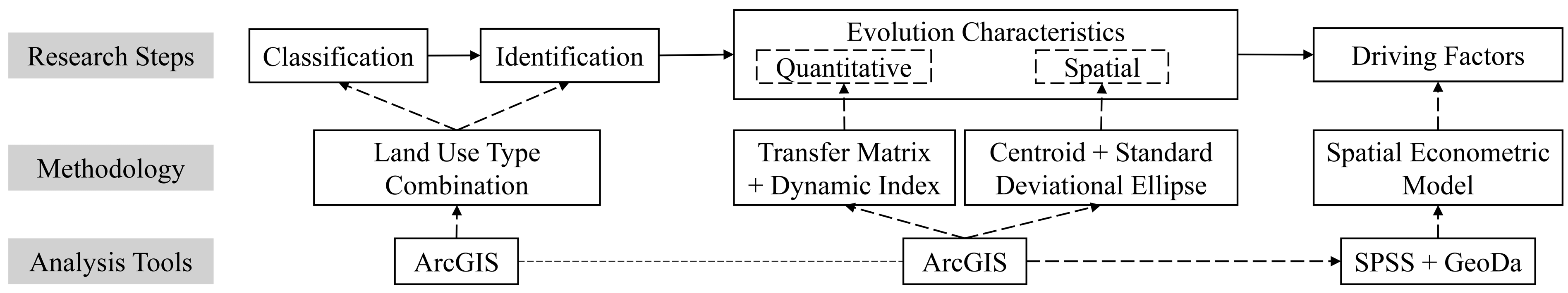
Therefore, this paper will take Chaoyang District of Beijing as an example to analyze land use changes and driving factors in the rural–urban fringe from the perspective of PLES (Figure 1). First, we used the land use type combination to identify PLES in the rural–urban fringe from 2005 to 2020. Second, we used the ArcGIS spatial analysis tools to analyze the evolution characteristics of PLES. Finally, we used the Spatial Econometric Model to analyze the driving factors of PLES.
3. Study Areas and Data
3.1. Study Areas
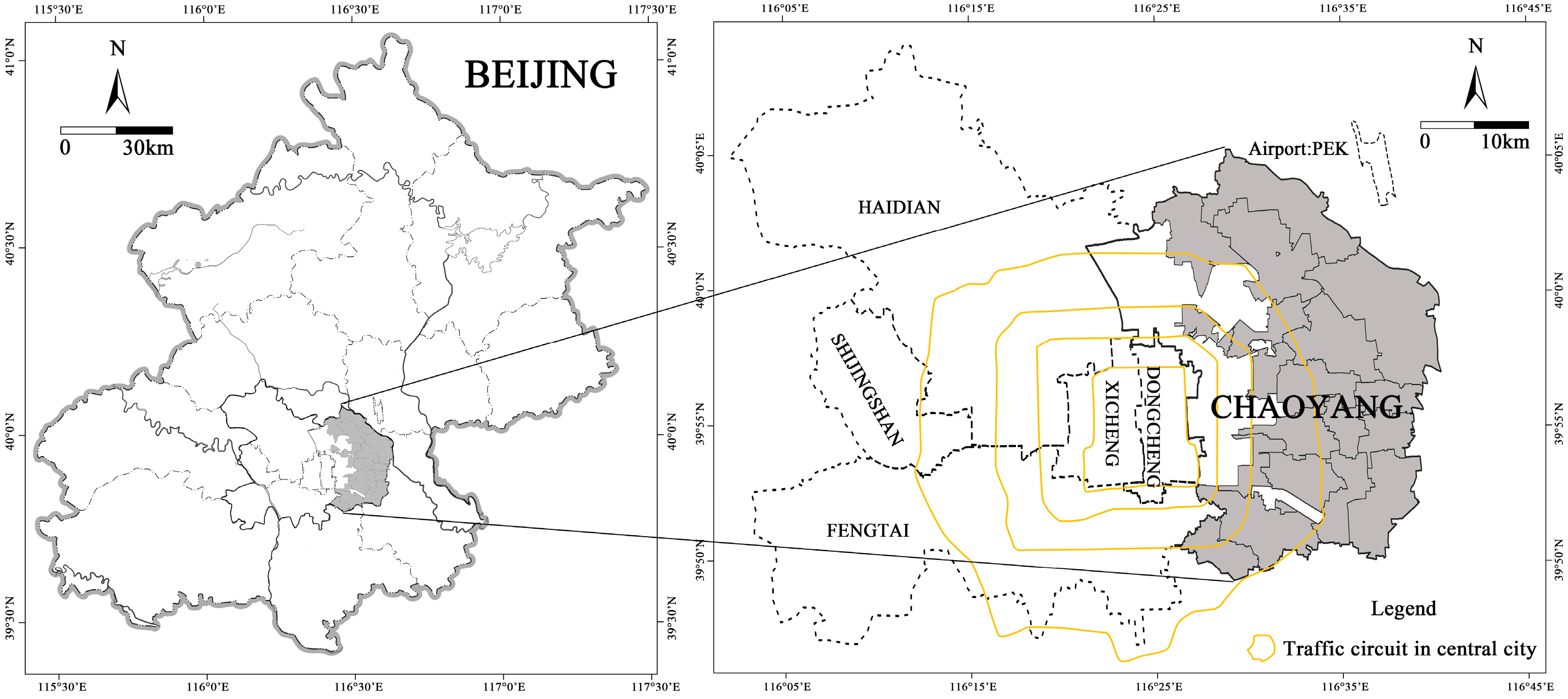
As the capital of China, Beijing is also one of the largest cities in China. Its urban area consists of Dongcheng, Xicheng, Chaoyang, Haidian, Fengtai, and Shijingshan Districts (Figure 2). In 2020, the total population of Beijing’s urban area exceed 10 million, and the area is 1381 km2. Beijing is a typical “Concentric Circle” spatial layout with several traffic circuits [17], and the structure of its rural–urban fringe is relatively clear. In the process of the development of the central city, the importance of the rural–urban fringe is increasing. Analyzing the spatial pattern evolution is of great significance for optimizing the urban spatial structure of the city, and promoting the economical use of land in the rural–urban fringe [3].
The study area of this paper included 169 villages, with a length of about 28 km from north to south and a width of about 15 km from east to west. In 2020, the total population was about 1.7 million, of which 950,000 could be considered a floating population. The study area was located in the east of central city, surrounding about half of the central city of Beijing, forming a relatively complete rural–urban fringe in space. In China’s urban–rural dual administrative system, the study area is classified as rural, which was significant to ensure the integrity of the research data. Since 2005, under the influence of the economic development of the central city and the expansion of built-up areas, the industrial structure, population composition, and land use have changed greatly, and the PLES of the study area has also changed.
3.2. Data Sources
The data used in this paper mainly included land use and socioeconomic data. The land use source data came from the Chinese Academy of Sciences Resource and Environmental Science Data Center (http://www.resdc.cn, accessed on 1 July 2021), with a spatial resolution of 30 m, which was based on Landsat TM images of the United States. In addition, it was generated by an artificial visual interpretation. On this basis, the source data were calibrated using the survey data of land change in Chaoyang District over the years, to improve its accuracy. The time span was from 2005 to 2020. Socioeconomic data sources included: “Chaoyang District Statistical Yearbook (2005–2020)”, “Chaoyang District National Economic and Social Development Statistical Bulletin (2005–2020)”, and “Chaoyang Rural Economic Data (2005–2021)”.
4. Methodology
4.1. PLES Classification
In this paper, the land use type combination was chosen to depict the PLES. First, combined with the characteristics of both agricultural and non-agricultural production in the rural–urban fringe, the traditional PLEF was divided into four functions: “Living, ecological, agricultural production, and non-agricultural production” [22]. Second, one land type usually had a variety of PLEFs, especially in China’s rural–urban fringe, where land use had a more evident mixed feature in the PLEF. Therefore, this paper drew on the concept of “compound functional space”, referring to various researchers regarding the classification system of Chinese PLES [41,43,44]. According to the PLEF of different land types, the PLES in the study area could be divided into “PS, ES, Eco-Agricultural Production Space (EAPS), Living-Agricultural Production Space (LAPS), and Living-Non-Farm Production Space (LNPS)” (Table 1).
For example, the basic function of cultivated land and garden land is agricultural production, but they also have certain ecological service functions. Therefore, agricultural land, such as cultivated land and garden land, was classified as EAPS. The basic function of commercial land is non-farm production, and it also has a certain living function. Therefore, it was classified as LNPS. Urban and rural residential land is mainly used for living function, with certain production functions at the same time. In China, urban residential land can be used for commercial rental, and rural residential land can also be used for agricultural production activity in the rural–urban fringe. Therefore, they were respectively classified as LNPS/LAPS. Transportation land is used for the construction of high-grade roads, railways, and supporting facilities, which mainly bears the function of non-agricultural production and agricultural production in the rural–urban fringe. Therefore, transportation land was classified as PS. The PLES classification of other land use types followed similar rules.
4.2. Space Patterns Transfer Matrix
The transfer matrix is often used to quantitatively analyze the direction and speed of land use change. The essence of the transfer matrix is to analyze the dynamic characteristics and trends of land use changes using the transition probability and stable state equation of Markov Chain. The demarcation of PLES is based on land use type. Therefore, the transfer matrix can also be used to analyze the quantitative characteristics of PLES evolution. The formula is as follows:
In the formula, i = 1, 2, …n; j = 1, 2, …n; n is the number of PLES. is the percentage of the total area converted from space type i to j in a certain period. is the percentage of total area of space type i that remains unchanged. can be further calculated, which is the percentage of space type i in the total area in the base period. represents the percentage of space type j in the total area in the final period. represents the percentage of space type i transferred out in the study period. is the percentage of the area transformed into space type j in the study period.
By analogy with the land use dynamic index, the space type dynamic index can be used to analyze the change speed and range of a certain PLES in the study period. The formula is as follows:
where K is the space type dynamic index, and are the area of a certain PLES in the base period and final period, respectively, and T is the duration of the study period.
4.3. Centroid and Standard Deviational Ellipse
The Centroid and Standard Deviational Ellipse are both classical spatial analysis tools, which can be used to describe the spatial characteristics of geographical elements, such as centrality, aggregation, and orientation. PLES is a patchy geographical element, and thus the Centroid and Standard Deviational Ellipse can describe the spatial pattern evolution of PLES in a more detailed way.
The Mean Center tool of ArcGIS can be used to calculate the centroid coordinates of different types of PLES at different times.
In the formula, and are the spatial coordinates of factor i, and are the average center of factor i, and n is the total number of patches.
The Standard Deviational Ellipse can describe the distribution direction and movement trend of PLES, and it includes the center of the circle, azimuth, major axis, and minor axis. The center of the ellipse is calculated using the arithmetic mean center:
Then, we can determine the direction of the ellipse by taking the X axis as the criterion, due north as 0 degrees, clockwise rotation, and azimuth calculation formula:
In the formula, and are the difference between the mean center and the xy coordinates.
Finally, we calculated the standard deviation of the XY axes as follows:
4.4. Spatial Econometric Model
Spatial econometric models are mainly divided into the Spatial Lag Model (SLM) and Spatial Error Model (SEM).
SLM is used to analyze the influence of dependent variables of adjacent regions on the dependent variables of this region, namely, the spatial spillover effect. The mathematical expression is:
In the formula, is the dependent variable, is the independent variable matrix, and reflects the influence of independent variable on the dependent variable . is the spatial lag dependent variable matrix, and is the spatial regression coefficient, reflecting the spatially dependent effect of sample observations. is a random error term vector and follows a normal distribution. is the spatial weight matrix based on geographical proximity, similar to what is shown below.
SEM is used to analyze the impact of the error term, which is the influence of the spatial correlation of unobservable factors in the adjacent region on the dependent variable in this region. The mathematical expression is:
where is the random error term vector, and is a spatial error coefficient, which measures the spatial dependence of sample observations. is a random error term vector, which obeys a normal distribution.
Performing the Lagrange Multiplier (LM) test on the estimation results of Ordinary Least Square Linear Regression (OLS), then, comparing Lagrange Multiplier (lag) and Lagrange Multiplier (error) of regression results, allowed us to select the appropriate model. If the former is statistically more significant than the latter, SLM will be selected. On the contrary, SEM is selected. If neither of them is significant, OLS is used.
Spatial autocorrelation analysis can be used for auxiliary analysis based on spatial data modeling. The Moran index can judge whether there is a significant correlation between the spatial internal elements. The value is within (−1, 1), with a value greater than 0 indicating a positive correlation, a value less than 0 indicating a negative correlation, and a value equal to 0 indicating no correlation.
4.5. Variable Selection
The rural–urban fringe supports diverse production and living activities of human beings, in which human factors evidently have an important impact on the evolution of PLES. In addition to the driving factors of land use changes confirmed in previous studies, this paper also focused on the effects of policy factors and distance factors. Since 2014, the main focus of urban planning for “Relocation of Non-Capital Functions” in Beijing has been adjusting the use of inefficient construction land and constructing urban parks to increase the greening rate. In this context, Chaoyang District, in accordance with the requirements of the Beijing Municipal government, issued a policy to select 12 townships (including 107 villages) as pilots to implement urbanization and greening construction (Pilot Township of Greenbelt). This policy may affect the evolution of PLES in the study area. As a part of the urban spatial structure, land use in the rural–urban fringe has been closely related to the urban development. Therefore, the evolution of PLES may also be related to the distance from the urban center.
Above all, in view of the actual situation and data availability of the study area, nine independent variables, including the urbanization rate of registered population and GDP, were selected from the dimensions of population, economic, industrial, and policies (Table 2). To avoid overly large differences in the magnitude of regression coefficients of independent variables, this study took logarithms of variables, such as “GDP, collective economic income, per capita fixed asset investment, and per capita labor income of farmers”. “Proportion of secondary industry” was the region’s industrial and manufacturing output as a share of GDP. “Distance from urban center” was the straight-line distance from the geometric center of the township to the urban center (Tian’anmen Square). The dependent variable was the space type with a large conversion area from 2005 to 2020, and the sample size was 169.
To determine the specific spatial econometric model, SPSS was first used to select independent variables. The selection of independent variables was based on Stepwise Regression. Entry and Removal in the stepwise probability were 0.05 and 0.10, respectively, indicating that when the p-value of the score test of the regression coefficient was less than 0.05, this variable would be included in the regression equation, and when the p-value was greater than 0.10, this variable would be excluded. According to the analysis results of SPSS, the number of independent variables of the four models was 7, 6, 6, 6, respectively. In the VIF test, the VIF values of all the variables were less than 5, and the average VIF value was 2.372. Therefore, errors caused by multicollinearity could be excluded.
Then, the Lagrange Multiplier (LM) test was performed on the OLS model estimation results (Table 3). Moran’s I (error) of dependent variables was significantly positive, indicating that in OLS regression models, their random error terms had different degrees of spatial positive correlation. Therefore, it was necessary to use the spatial econometric model to analyze driving factors. Comparing the p-value of LM lag and LM error, SLM should be used for the dependent variables space-v1 and space-v2. Accordingly, SEM should be adopted for dependent variables space-v3 and space-v4. For testing the fitting effect of the spatial econometric model, in addition to the Coefficient of Determination test, the Log Likelihood (log-L), Akaike Information Criterion (AIC), and Schwartz Criterion (SC) are used, among other indicators. The judgment criterion is that the larger the log-L, the smaller the AIC and SC, and the better the model fitting effect [49].
5. Results
5.1. How Has the PLES Evolved?
5.1.1. Type Conversion of PLES
According to the transfer matrix and space type dynamic index of PLES (Table 4), from 2005 to 2010, the conversion scale of PLES was the largest. The area of PS which turned into LNPS reached 2409.73 hm2, accounting for 18.24% of the turn-out space. PS was supplemented by ES, EAPS, and LAPS at the same time, and its area increased slightly. From the perspective of the space type dynamic index, the change of LNPS was the most evident, with an average annual growth rate of 31.9%. EAPS mainly turned into PS and ES, while LAPS mainly turned into PS and LNPS, with an annual decrease of 4.88% and 7.81%, respectively. From 2010 to 2015, the conversion scale of PLES was the smallest. The area of PS which turned into LNPS reached 1303.57 hm2, accounting for 20.27% of the turn-out space. However, as it was supplemented by ES and EAPS, the area of PS decreased only slightly, with an annual decrease of 0.32%. LNPS continued to expand, but the annual growth rate dropped to 8.42%. EAPS and LAPS continued to shrink. From 2015 to 2020, the conversion of PS to LNPS was still the main direction observed, with a conversion area of 2152.45 hm2, accounting for 36.38% of the turn-out space. In addition, the PS area began to shrink, with an annual decrease of 4.31%. ES was mainly supplemented by PS and EAPS, with an average annual growth rate of 4.25%.
In general, from 2005 to 2020, the areas of EAPS and LAPS have been shrinking, and the space type dynamic index values were –3.69 and –5.27, respectively. On the contrary, LNPS continued to receive large-scale turn-in from other types of PLES, with an average annual growth rate of 27.04%. By 2020, it had become the largest space type in the study area, accounting for 35.52%. PS first increased and then decreased, while ES first decreased and then increased, especially during the period from 2015 to 2020, when PS decreased significantly and ES continued to expand. In the whole study period, the space type dynamic index values of the two were –1.42 and 2.59, respectively.
In analyzing the details of the conversion of PLES, the main conversion direction of PLES was found to be from PS to LNPS in the periods of 2005–2010, 2010–2015, and 2015–2020, and its proportion in the total conversion area gradually increased from 18.24% to 36.38%. A comprehensive analysis pattern evolution of PLES found that the urbanization mode of the study area was different from the traditional “Agricultural/Rural residential land→Urban construction land” path, showing instead the “Agricultural/Rural residential land→Industrial land→Urban construction land” three-phase path. The typical characteristic that industrialization drives urbanization development was confirmed.
In addition, from 2010 to 2015, the minor direction of conversion was from EAPS to ES, accounting for 12.42% of the conversion area. From 2015 to 2020, the minor direction was from PS to ES, accounting for 14.69% of the conversion area. The scale of ES gradually expanded, indicating that the ecological environment protection in the study area has been paid increasing attention. This may also be related to the fact that Beijing began to implement the “Relocation of Non-Capital Functions” in 2014, which significantly reduced the proportion of industrial production, and improved the ecological environment quality in the downtown and rural–urban fringe areas [10].
5.1.2. Spatial Characteristics of PLES
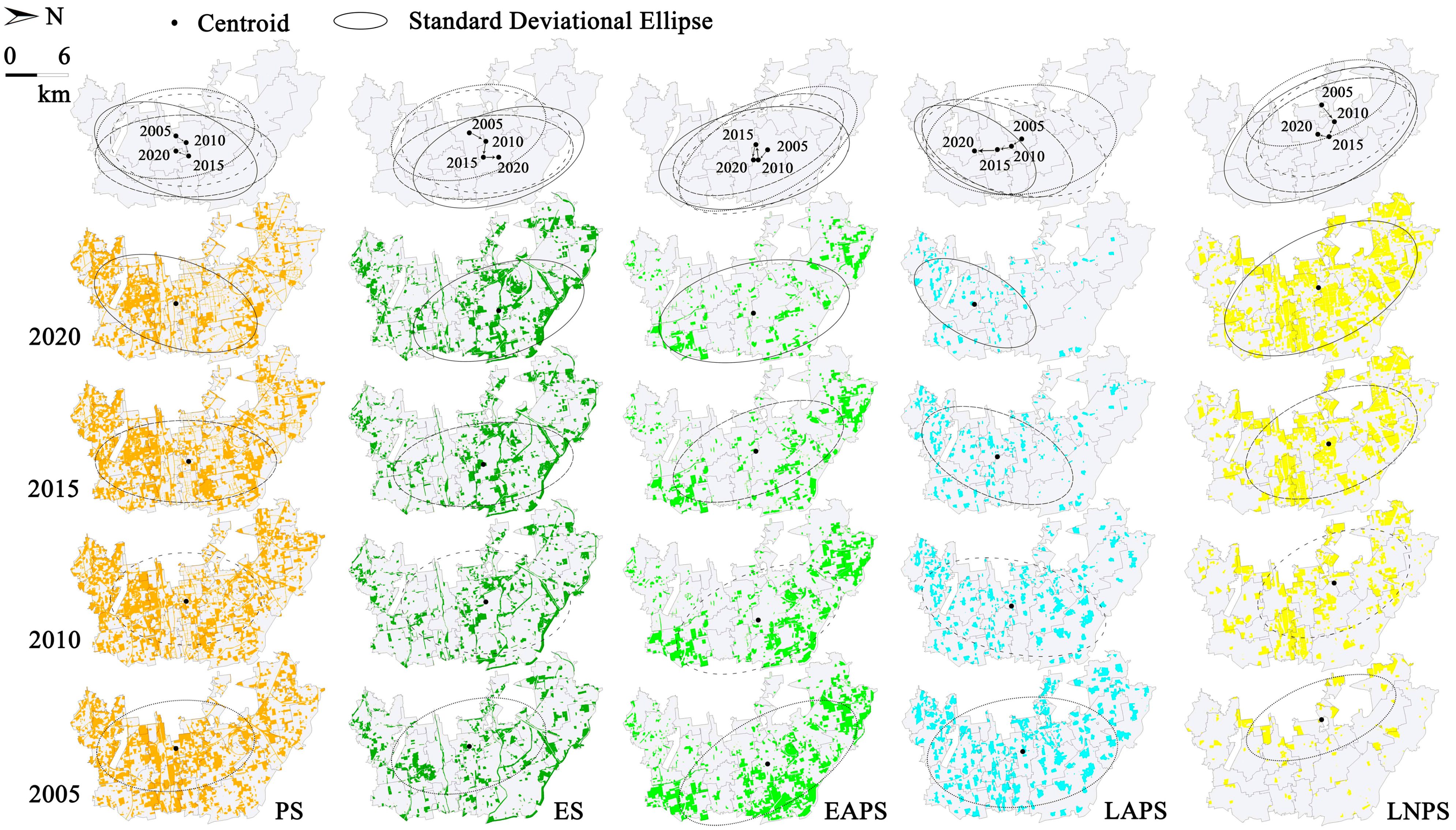
By describing the centroid and standard deviation ellipses, the evolution path and expansion direction of PLES could be clearly displayed (Figure 3). They have the following characteristics:
- (1)
- PS presented a trend of location offshoring, spatial aggregation, and scale reduction. In 2005, PS in the study area was relatively intensively distributed. Since then, with the expansion of LNPS, PS has moved outward to the fringe of the city, shrinking in scale. By 2020, PS was mainly concentrated in the south-central and eastern townships. From 2005 to 2010, the centroid of PS was mainly concentrated in the middle of the study area, and the long axis of the standard deviation ellipse was north–south. From 2010 to 2015, the centroid of PS gradually moved to the northeast, and the ellipse moved along with it. The ratio of long and short axis increased, indicating that PS was showing a trend of expanding to the fringe of the city. From 2015 to 2020, the centroid moved to the southwest direction, and the long axis of the ellipse shifted to the northeast–southwest direction, since PS in the northern area was significantly reduced.
- (2)
- The scale of ES decreased first and then increased, and gradually formed an ecological spatial ring in the eastern region. There were two stages of ES conversion. From 2005 to 2010, ES showed a shrinking trend, especially in the central and southern areas. Thereafter, ES in the south recovered slightly, while in the north, it continued to increase. The scattered ES gradually connected dots into lines, with a slight increase in scale. By 2020, ES was mainly distributed in the central, northern, and eastern fringe of the study area, forming a green ecological landscape belt. The trend of ES expansion to the northeast was evident. From 2005 to 2020, the centroid of ES moved to the northeast, the long axis of the standard deviation ellipse presented a northwest-southeast direction, and the ratio of the long and short axis gradually increased.
- (3)
- EAPS was rapidly reduced in the spatial order from near-to-far from the city center. In 2005, EAPS was mainly distributed in the north, northeast, and southeast. With the expansion of LNPS and offshoring of PS, EAPS was shrinking from inside to outside and from west to east, especially in the period of 2005–2015, when its scale reduced evidently. By 2020, only a few areas in the north, east, and southeast remained as a small-scale EAPS. From 2005 to 2020, the centroid of EAPS was concentrated in the middle and north, and the long axis of the standard deviation ellipse was in the northwest-southeast direction. Specifically, from 2005 to 2010, the centroid and ellipse moved to the southeast, and the ratio of the long and short axis decreased. Thereafter, the centroid and ellipse moved to the east, indicating that the reduction of EAPS in the study area had a trend of extending from west to east to the outskirts of the city.
- (4)
- LAPS shrank from a patchy distribution to almost disappearing. In 2005, LAPS in the study area was scattered in patches, and the scale was relatively large, exceeding the ES. With the expansion of LNPS, LAPS, carrying the rural life function, shrunk. By 2020, only a small amount of LAPS remained in the southern region, indicating that there was still some rural residential areas that had not yet been urbanized. From 2005 to 2020, the expansion direction of LAPS followed an evident law, in which the centroid continued to move southward, the long axis of standard deviation ellipse gradually changed from south–north to northeast–southwest, and the ellipse continued to shrink. In 2005, the distribution of LAPS was relatively uniform, and the centroid was located in the middle of the study area. Since then, the scale of LAPS has been shrinking, and the speed of shrinking in the north has been significantly faster than in the south. By 2020, LAPS in the north had basically disappeared.
- (5)
- LNPS expanded rapidly in the spatial order of the point-line-plane, and from near-to-far from the city center. In 2005, LNPS in the study area was concentrated in the central and northern areas near the urban center, with a spotty distribution. From 2005 to 2010, LNPS was extended and expanded in two directions: East and northeast, leading to the sub-center of Beijing (Tongzhou District) and the Capital Airport, respectively. Since then, LNPS has gradually expanded from inside to outside, and by 2020, it had become the largest space type in the study area. From 2005 to 2020, the centroid of LNPS moved to the northeast first, then to the southeast, and finally to the south. The long axis of the standard deviation ellipse mainly showed a northwest-southeast direction, and the ellipse continued to expand. Specifically, from 2005 to 2010, LNPS expanded to the northeast, and the ratio of the long and short axis increased. Thereafter, LNPS continued to expand eastward, with a more balanced spatial distribution on the whole.
5.2. What Drives the Conversion?
5.2.1. PS Conversion
Based on the spatial econometric analysis results (Table 5), from 2005 to 2020, PS→LNPS (space-v1) was the main conversion direction, accounting for 24.98% of the total conversion area. Its positive driving factors included the “urbanization rate, GDP, collective economic income, and per capita fixed asset investment”. “Proportion of secondary industry and distance from urban center” had a significant negative driving force on space conversion, indicating that the lower the proportion of the secondary industry output value or the closer the distance to the city center, the easier it was for PS to turn into LNPS. The conversion of “PS→ES” (space-v4) was 1316.20 hm2, accounting for 7.05% of the total conversion area. The positive driving factors were “Pilot Township of greenbelt and distance from urban center”, and “population density, collective economic income, and proportion of secondary industry” were significant negative driving forces.
The conversion of PS to LNPS is an important symbol of urbanization driven by industrialization, which needs to be driven by economic growth and industrial transformation and upgrading [50]. In previous studies, the urbanization rate, GDP, and per capita fixed asset investment had significant positive driving effects on the reduction of agricultural land or expansion of construction land [51]. This study further confirmed that the above factors further drove PS to LNPS. Beijing has a typical “Concentric Circle” spatial structure. The study area is located in the east of the city center, which was mainly used for the development of agriculture and light industry around 2005. Since then, as the city center has spread outward, Beijing has continuously reduced the proportion of industrial production in the city’s economy, eliminated inefficient and highly polluting industrial projects, developed tertiary industries, and increased economic growth and the urbanization rate. These factors drove the conversion of PS in the rural–urban fringe to LNPS.
The conversion of PS to ES is an important symbol of deindustrialization. The farther away from the city center, the greater the driving force for space conversion. The driving effect of “distance from urban center” on the conversion of PS to LNPS and ES was opposite to this. Since 2014, the Beijing Municipal government has systematically engaged in “Relocation of Non-Capital Functions”, eliminated backward industries in the rural–urban fringe, and dispersed the unskilled floating population living there. The lower the income of the collective economy, the more favorable it was for PS to turn into ES. This was due to the fact that in the process of “Relocation of Non-Capital Functions”, rural collective industries with small enterprises and low economic benefits would be preferentially eliminated, then the industrial land was used for greening. In this context, the policy of “Pilot Township of Greenbelt” was aimed at promoting complete urbanization in the rural–urban fringe, and at the same time promoting the regional economic development and expanding the scale of green land. The analysis results also confirmed that this policy significantly drove the conversion of PS to ES.
5.2.2. EAPS Conversion
EAPS was mainly converted to ES and LNPS, with conversion areas of 1988.84 and 1739.52 hm2, respectively. For EAPS→ES (space-v2), the positive driving factors included “GDP, collective economic income, per capita labor income of farmers, Pilot Township of greenbelt, and distance from urban center”. For EAPS→LNPS (space-v3), the positive driving factors included the “urbanization rate, GDP, income-CE, and per capita labor income of farmers”, and “distance from urban center” had a significant negative driving force on space conversion.
The essence of EAPS→ES is the conversion of agricultural land to ecological land, such as grassland and forest land, which is an important embodiment of regional ecological construction and is conducive to the protection and improvement of the ecological environment [52]. This kind of space conversion was related to the regional economic strength, especially for the rural–urban fringe, where there was a mixed urban economy and rural economy. The higher the collective economic income and farmers’ income, the more conducive driving this space conversion was, thus promoting the expansion of ES. The policy of “Pilot Township of greenbelt” showed a significant driving force as well, which was similar to the policy effect of the conversion of PS to ES. The closer it was to the city center, the more favorable it was for this space conversion to occur, which was in line with the spatial characteristics of Beijing city expanding from inside to outside.
EAPS→LNPS is the conversion of agricultural land, such as cultivated land and garden land, to urban residential land, which is an important embodiment of urbanization. In previous studies, the urbanization rate, GDP, and other factors had significant positive driving effects on construction land expansion [53], and this was further confirmed in this study. Collective economic income and per capita labor income of farmers had a positive driving effect on this space conversion, since in the rural–urban fringe, most of the farmers hope to improve their living environment through urbanization. In addition, villages with high collective economic income are better able to achieve farmers’ goals. The farther away from the central city, the more conducive conditions were to space conversion. From the perspective of land cost, expansion of ES in the rural–urban fringe usually required the government to expropriate agricultural land for greening. Within a certain range, the farther away from the central city, the lower the cost of land, and the more beneficial it was to increase ES.
6. Conclusions
The introduction of the PLES research perspective, exploring the law of land use changes in the rural–urban fringe, and analyzing the driving factors of the evolution of PLES, has been helpful in using spatial planning to optimize the allocation of land resources, strengthen urban border controls, clear regional development pathways, and improve spatial governance in the rural–urban fringe. This paper took the Chaoyang District of Beijing as an example, and the research period was 2005–2020. Based on the identification and characterization of PLES evolution, this paper optimized the spatial econometric model to analyze the driving factors of space conversion. The main conclusions are:
- Stage characteristics of PLES conversion: From 2005 to 2010, the conversion scale of PLES was the largest. From 2005 to 2020, PS→LNPS was the primary direction of PLES conversion. LNPS continued to receive a large inflow and gradually increased as the largest PLES type in the study area. EAPS and LAPS were in a state of net outflow, and their area was shrinking. Since 2010, the scale of ES had gradually expanded, mainly to obtain EAPS and PS inflow.
- On the evolution of PLES: From 2005 to 2020, PS showed a trend of location offshoring, spatial aggregation, and scale reduction. The scale of ES decreased first and then increased, forming a green ecological landscape belt on the periphery of Beijing. EAPS was rapidly reduced in the spatial order from near-to-far from the city center. LAPS shrank from a patchy distribution until it almost disappeared. LNPS expanded rapidly in the spatial order of the point-line-plane, and from near-to-far from the city center.
- Driving factors of PLES evolution: From 2005 to 2020, the conversion of PS→LNPS was an important symbol of industrialization-driven urbanization, which needed to be jointly driven by economic growth and industrial transformation and upgrading. The conversion of PS→ES was an important symbol of deindustrialization. Affected by population density and the industrial structure, the driving effect of distance on the conversion of PS to LNPS and ES was the opposite. The conversion of EAPS→ES was an important reflection of regional ecological construction, which was conducive to the protection of the ecological environment. Driven by rural economic strength, the driving effect of the “Pilot Township of greenbelt” policy was significant, which was similar to the policy effect of the conversion of PS→ES. EAPS→LNPS was an important indicator of urbanization construction. Driven by the urbanization rate and economic strength, distance had a significant negative driving force on these two types of space conversions.
7. Discussion
Land use is closely related to regional development. PLES, based on the PLEF of the land use type, can reflect regional development characteristics to a certain extent. According to the analysis results of the evolution of PLES, from 2005 to 2020, EAPS and LAPS in Beijing’s rural–urban fringe decreased, while LNPS expanded significantly, representing the process of rapid urbanization. In addition, the urbanization pathway of this region showed the evolution process of “LAPS/EAPS→PS→LNPS”, which has the characteristic of industrialization driving urbanization development. This is similar to some developing countries, since under the development strategy of high economic growth and environmental protection, it is necessary to sacrifice rural land in the rural–urban fringe [54], such as Vietnam and the Philippines [55]. However, in developed countries, due to strict planning restrictions, land use in the rural–urban fringe changes slowly and is difficult to be used for industrial construction [56].
In previous studies, factors such as economic growth and industrial transformation and upgrading had a significant driving effect on the reduction of agricultural land or expansion of construction land. This paper confirmed that relevant factors will further drive the conversion of PS to LNPS, and realize industrialization to drive urbanization. We found that the collective economy had a significant impact on land use change in the rural–urban fringe, and a similar phenomenon exists in Israel and Vietnam [55,57], since their rural mode of production has a certain collectivity. “Pilot Township of greenbelt” is an important policy for Beijing to adjust its urban development strategy and restore the ecological landscape in the rural–urban fringe. This study confirmed that, in the PLES evolution process, this policy has a significant driving effect on the conversion of PS/EAPS to ES. In London and other European cities, greenbelt also has a significant impact on land use change in the rural–urban fringe [58]. Beijing has a typical “Concentric Circle” spatial structure, and “distance from urban center” has an important impact on the evolution of PLES in the rural–urban fringe. Studies have proven that the closer the distance to the city center, the more conducive the conversion of other PLESs to LNPS, and the further the distance from the city center, the more conducive the conversion of other PLESs to ES. Most of the cities in China are marginal expansion patterns, and land use in the rural–urban fringe is affected by the central city to varying degrees [59]. The “Concentric Circle” spatial structure of Beijing may make this driving effect more significant.
There are also some limitations in this paper. The scientific definition of PLEF and the standard of PLES division need to be discussed more fully, and the regularity summary of the spatial pattern evolution needs to be strengthened. The central city has an important influence on the land use in the rural–urban fringe. Considering the spatial structure of Beijing, this paper only set the distance variable and verified the distance effect, and there may be other more complex driving mechanisms. In addition, due to space limitations, this paper analyzed the driving factors of four main types of space conversions. However, the driving factors of other types of space conversions need to be further studied.
Author Contributions
Conceptualization, C.F. and H.Z.; methodology, C.F. and H.Z.; software, H.Z.; investigation, L.X. and Y.G.; resources, Y.G.; writing—original draft preparation, C.F. and H.Z.; writing—review and editing, H.Z.; visualization, H.Z.; supervision, L.X. and Y.G.; funding acquisition, C.F. All authors have read and agreed to the published version of the manuscript.
Funding
This research was funded by the National Key R&D Program of China, grant number 2019YFD1100802.
Institutional Review Board Statement
Not applicable.
Informed Consent Statement
Not applicable.
Data Availability Statement
The data presented in this study are available on request from the author.
Conflicts of Interest
The authors declare no conflict of interest.
Abbreviations
The following table shows the abbreviations used in this article.
| PLES | Production–Living–Ecological Space | PLEF | Production–Living–Ecological Function |
| PS | Production Space | LAPS | Living-Agricultural Production Space |
| LS | Living Space | LNPS | Living-Non-Farm Production Space |
| ES | Ecological Space | EAPS | Eco-Agricultural Production Space |
| GTWR | Geographically and Temporally Weighted Regression | GWR | Geographically Weighted Regression |
| SLM | Spatial Lag Model | SEM | Spatial Error Model |
| LM | Lagrange Multiplier | Log-L | Log Likelihood |
| AIC | Akaike Information Criterion | SC | Schwartz Criterion |
References
- Liu, Y.; Huang, X.; Yang, H.; Zhong, T. Environmental effects of land-use/cover change caused by urbanization and policies in Southwest China Karst area—A case study of Guiyang. Habitat Int. 2014, 44, 339–348. [Google Scholar] [CrossRef]
- Zhang, L.; Wang, S.X.; Yu, L. Is social capital eroded by the state-led urbanization in China? A case study on indigenous villagers in the urban fringe of Beijing. China Econ. Rev. 2015, 35, 232–246. [Google Scholar] [CrossRef]
- Zhao, P. Too complex to be managed? New trends in peri-urbanisation and its planning in Beijing. Cities 2013, 30, 68–76. [Google Scholar] [CrossRef]
- Zhao, P.; Wan, J. Land use and travel burden of residents in urban fringe and rural areas: An evaluation of urban-rural integration initiatives in Beijing. Land Use Policy 2021, 103, 105309. [Google Scholar] [CrossRef]
- Liu, R.; Tai-chee, W.; Liu, S. The informal housing market in Beijing’s rural areas: Its formation and operating mechanism amidst the process of urbanization. Geogr. Res. 2010, 29, 1355–1358. [Google Scholar]
- Sun, L.; Fertner, C.; Jorgensen, G. Beijing’s First Green Belt—A 50-Year Long Chinese Planning Story. Land 2021, 10, 969. [Google Scholar] [CrossRef]
- Liu, D.; Zheng, X.; Wang, H.; Zhang, C.; Li, J.; Lv, Y. Interoperable scenario simulation of land-use policy for Beijing-Tianjin-Hebei region, China. Land Use Policy 2018, 75, 155–165. [Google Scholar] [CrossRef]
- Shi, W.; He, C.; Hu, B.; Peng, K. Following the national strategy, responding to the call of age: Several key points in new Beijing city master plan. City Plan. Rev. 2017, 41, 17–22. [Google Scholar]
- Duan, Y.; Wang, H.; Huang, A.; Xu, Y.; Lu, L.; Ji, Z. Identification and spatial-temporal evolution of rural “production-living-ecological” space from the perspective of villagers’ behavior—A case study of Ertai Town, Zhangjiakou City. Land Use Policy 2021, 106, 105457. [Google Scholar] [CrossRef]
- Wiggering, H.; Dalchow, C.; Glemnitz, M.; Helming, K.; Muller, K.; Schultz, A.; Stachow, U.; Zander, P. Indicators for multifunctional land use—Linking socio-economic requirements with landscape potentials. Ecol. Indic. 2006, 6, 238–249. [Google Scholar] [CrossRef]
- Jing, W.; Yu, K.; Wu, L.; Luo, P. Potential Land Use Conflict Identification Based on Improved Multi-Objective Suitability Evaluation. Remote Sens. 2021, 13, 2416. [Google Scholar] [CrossRef]
- Zhou, W.; Jiao, M.; Yu, W.; Wang, J. Urban sprawl in a megaregion: A multiple spatial and temporal perspective. Ecol. Indic. 2019, 96, 54–66. [Google Scholar] [CrossRef]
- Peiser, R.B. Does it pay to plan suburban growth. J. Am. Plan. Assoc. 1984, 50, 419–433. [Google Scholar] [CrossRef]
- Sutton, P.C. A scale-adjusted measure of “Urban sprawl” using nighttime satellite imagery. Remote Sens. Environ. 2003, 86, 353–369. [Google Scholar] [CrossRef]
- Bontje, M.; Burdack, J. Edge Cities, European-style: Examples from Paris and the Randstad. Cities 2005, 22, 317–330. [Google Scholar] [CrossRef]
- Myers, R.R.; Beegle, J.A. Delineation and analysis of the rural-urban fringe. Appl. Anthropol. 1947, 6, 14–22. [Google Scholar] [CrossRef]
- Zhao, P. Managing urban growth in a transforming China: Evidence from Beijing. Land Use Policy 2011, 28, 96–109. [Google Scholar] [CrossRef]
- Long, H.; Liu, Y.; Hou, X.; Li, T.; Li, Y. Effects of land use transitions due to rapid urbanization on ecosystem services: Implications for urban planning in the new developing area of China. Habitat Int. 2014, 44, 536–544. [Google Scholar] [CrossRef]
- Liu, Y.; Long, H.; Li, T.; Tu, S. Land use transitions and their effects on water environment in Huang-Huai-Hai Plain, China. Land Use Policy 2015, 47, 293–301. [Google Scholar] [CrossRef]
- Wei, Y.D.; Ewing, R. Urban expansion, sprawl and inequality. Landsc. Urban Plan. 2018, 177, 259–265. [Google Scholar] [CrossRef]
- Anderson, W.P.; Kanaroglou, P.S.; Miller, E.J. Urban form, energy and the environment: A review of issues, evidence and policy. Urban Stud. 1996, 33, 7–35. [Google Scholar] [CrossRef]
- Li, G.; Cao, Y.; He, Z.; He, J.; Wang, J.; Fang, X. Understanding the Diversity of Urban-Rural Fringe Development in a Fast Urbanizing Region of China. Remote Sens. 2021, 13, 2373. [Google Scholar] [CrossRef]
- Thapa, R.B.; Murayama, Y. Drivers of urban growth in the Kathmandu valley, Nepal: Examining the efficacy of the analytic hierarchy process. Appl. Geogr. 2010, 30, 70–83. [Google Scholar] [CrossRef]
- Vu, T.; Shen, Y. Land-Use and Land-Cover Changes in Dong Trieu District, Vietnam, during Past Two Decades and Their Driving Forces. Land 2021, 10, 798. [Google Scholar] [CrossRef]
- Feng, Y.; Tong, X. Using exploratory regression to identify optimal driving factors for cellular automaton modeling of land use change. Environ. Monit. Assess. 2017, 189, 515. [Google Scholar] [CrossRef]
- Badmos, B.K.; Villamor, G.B.; Agodzo, S.K.; Odai, S.N.; Badmos, O.S. Local level impacts of climatic and non-climatic factors on agriculture and agricultural land-use dynamic in rural northern Ghana. Singap. J. Trop. Geogr. 2018, 39, 178–191. [Google Scholar] [CrossRef]
- Chen, M.; Lu, Y.; Ling, L.; Wan, Y.; Luo, Z.; Huang, H. Drivers of changes in ecosystem service values in Ganjiang upstream watershed. Land Use Policy 2015, 47, 247–252. [Google Scholar] [CrossRef]
- Heilig, G.K. Anthropogenic factors in land-use change in China. Popul. Dev. Rev. 1997, 23, 139–168. [Google Scholar] [CrossRef] [Green Version]
- Nyamekye, C.; Kwofie, S.; Ghansah, B.; Agyapong, E.; Boamah, L.A. Assessing urban growth in Ghana using machine learning and intensity analysis: A case study of the New Juaben Municipality. Land Use Policy 2020, 99, 105057. [Google Scholar] [CrossRef]
- Yansui, L.; Shasha, L.; Yufu, C. Spatio-temporal change of urban-rural equalized development patterns in China and its driving factors. J. Rural Stud. 2013, 32, 320–330. [Google Scholar]
- Lopez, E.; Bocco, G.; Mendoza, M.; Velazquez, A.; Aguirre-Rivera, J.R. Peasant emigration and land-use change at the watershed level: A GIS-based approach in Central Mexico. Agric. Syst. 2006, 90, 62–78. [Google Scholar] [CrossRef]
- Jiang, L.; Zhang, Y. Modeling Urban Expansion and Agricultural Land Conversion in Henan Province, China: An Integration of Land Use and Socioeconomic Data. Sustainability 2016, 8, 920. [Google Scholar] [CrossRef] [Green Version]
- Fan, X.; Zhao, L.; He, D. Land Use Changes and its Driving Factors in a Coastal Zone. Pol. J. Environ. Stud. 2020, 29, 1143–1150. [Google Scholar] [CrossRef]
- Peng, Y.; Yang, F.; Zhu, L.; Li, R.; Wu, C.; Chen, D. Comparative Analysis of the Factors Influencing Land Use Change for Emerging Industry and Traditional Industry: A Case Study of Shenzhen City, China. Land 2021, 10, 575. [Google Scholar] [CrossRef]
- Lubowski, R.N.; Plantinga, A.J.; Stavins, R.N. What Drives Land-Use Change in the United States? A National Analysis of Landowner Decisions. Land Econ. 2008, 84, 529–550. [Google Scholar] [CrossRef]
- Song, X. Discussion on land use transition research framework. Acta Geogr. Sin. 2017, 72, 471–487. (In Chinese) [Google Scholar]
- Peng, J.; Zhao, M.; Guo, X.; Pan, Y.; Liu, Y. Spatial-temporal dynamics and associated driving forces of urban ecological land: A case study in Shenzhen City, China. Habitat Int. 2017, 60, 81–90. [Google Scholar] [CrossRef]
- Holloway, G.; Lacombe, D.; LeSage, J.P. Spatial econometric issues for bio-economic and land-use modelling. J. Agric. Econ. 2007, 58, 549–588. [Google Scholar] [CrossRef]
- Huang, B.; Wu, B.; Barry, M. Geographically and temporally weighted regression for modeling spatio-temporal variation in house prices. Int. J. Geogr. Inf. Sci. 2010, 24, 383–401. [Google Scholar] [CrossRef]
- Wu, J.; Luo, K.; Zhao, Y. The evolution of urban landscape pattern and its driving forces of Shenzhen from 1996 to 2015. Geogr. Res. 2020, 39, 1725–1738. (In Chinese) [Google Scholar]
- Lin, G.; Fu, J.; Jiang, D. Production-Living-Ecological Conflict Identification Using a Multiscale Integration Model Based on Spatial Suitability Analysis and Sustainable Development Evaluation: A Case Study of Ningbo, China. Land 2021, 10, 383. [Google Scholar] [CrossRef]
- Zhou, D.; Xu, J.; Lin, Z. Conflict or coordination? Assessing land use multi-functionalization using productionliving-ecology analysis. Sci. Total Environ. 2017, 577, 136–147. [Google Scholar] [CrossRef]
- Zhang, X.; Xu, Z. Functional Coupling Degree and Human Activity Intensity of Production-Living-Ecological Space in Underdeveloped Regions in China: Case Study of Guizhou Province. Land 2021, 10, 56. [Google Scholar] [CrossRef]
- Yang, Y.; Bao, W.; Li, Y.; Wang, Y.; Chen, Z. Land Use Transition and Its Eco-Environmental Effects in the Beijing-Tianjin-Hebei Urban Agglomeration: A Production-Living-Ecological Perspective. Land 2020, 9, 285. [Google Scholar] [CrossRef]
- Tian, F.; Li, M.; Han, X.; Liu, H.; Mo, B. A Production-Living-Ecological Space Model for Land-Use Optimisation: A case study of the core Tumen River region in China. Ecol. Model. 2020, 437, 109310. [Google Scholar] [CrossRef]
- Carrion-Flores, C.; Irwin, E.G. Determinants of residential land-use conversion and sprawl at the rural-urban fringe. Am. J. Agric. Econ. 2004, 86, 889–904. [Google Scholar] [CrossRef]
- Chen, Z.; Lu, C.; Fan, L. Farmland changes and the driving forces in Yucheng, North China Plain. J. Geogr. Sci. 2012, 22, 563–573. [Google Scholar] [CrossRef] [Green Version]
- Shi, Z.; Deng, W.; Zhang, S. Spatio-temporal pattern changes of land space in Hengduan Mountains during 1990–2015. J. Geogr. Sci. 2018, 28, 529–542. [Google Scholar] [CrossRef] [Green Version]
- Li, T.; Long, H.; Liu, Y.; Tu, S. Multi-scale analysis of rural housing land transition under China’s rapid urbanization: The case of Bohai Rim. Habitat Int. 2015, 48, 227–238. [Google Scholar] [CrossRef]
- Iwata, O.; Oguchi, T. Factors Affecting Late Twentieth Century Land Use Patterns in Kamakura City, Japan. Geogr. Res. 2009, 47, 175–191. [Google Scholar] [CrossRef]
- Han, H.R.; Yang, C.F.; Song, J.P. The spatial-temporal characteristic of land use change in Beijing and its driving mechanism. Econ. Geogr. 2015, 35, 148–154. (In Chinese) [Google Scholar]
- Liu, R.; Liu, X.M. Analysis on Spatial-Temporal Changes and Driving Forces of “Production-Living-Ecological” Spaces in Beijing-Tianjin-Hebei Metropolitan Area. Ecol. Econ. 2021, 37, 201–208. (In Chinese) [Google Scholar]
- Song, J.; Zhao, X.; Wang, Q. Analysis of Land Use Change and Socioeconomic Driving Forces of Fengtai District in Beijing. China Popul. Resour. Environ. 2008, 18, 171–175. (In Chinese) [Google Scholar]
- Wadduwage, S. Peri-urban agricultural land vulnerability due to urban sprawl: A muiti-criteria spatially-explicit scenario analysis. J. Land Use Sci. 2018, 13, 358–374. [Google Scholar] [CrossRef] [Green Version]
- Nguyen, Q.; Kim, D.C. Reconsidering rural land use and livelihood transition under the pressure of urbanization in Vietnam: A case study of Hanoi. Land Use Policy 2020, 99, 104896. [Google Scholar] [CrossRef]
- Saizen, I.; Mizuno, K.; Kobayashi, S. Effects of land-use master plans in the metropolitan fringe of Japan. Landsc. Urban Plan. 2006, 78, 411–421. [Google Scholar] [CrossRef]
- Bittner, C.; Sofer, M. Land use changes in the rural-urban fringe: An Israeli case study. Land Use Policy 2013, 33, 11–19. [Google Scholar] [CrossRef]
- Gant, R.L.; Robinson, G.M.; Fazal, S. Land-use change in the ‘edgelands’: Policies and pressures in London’s rural-urban fringe. Land Use Policy 2011, 28, 266–279. [Google Scholar] [CrossRef]
- Cheng, C.; Yang, X.; Cai, H. Analysis of Spatial and Temporal Changes and Expansion Patterns in Mainland Chinese Urban Land between 1995 and 2015. Remote Sens. 2021, 13, 2090. [Google Scholar] [CrossRef]
Figure 1.
Research framework and steps.

Figure 2.
Location of the study area in Beijing.

Figure 3.
Centroid migration and standard deviation ellipse of PLES.


Table 1.
PLEF and PLES classification of different land use types.
| Land Use Types/PLEF | Living | Ecological | Agricultural Production | Non-Agricultural Production | PLES |
|---|---|---|---|---|---|
| Cultivated land | √ | √ | EAPS | ||
| Garden land | √ | √ | EAPS | ||
| Forest land | √ | ES | |||
| Grassland | √ | ES | |||
| Commercial land | √ | √ | LNPS | ||
| Industrial/Warehouse land | √ | PS | |||
| Urban residential land | √ | √ | LNPS | ||
| Rural residential land | √ | √ | LAPS | ||
| Public management land | √ | √ | LNPS | ||
| Transportation land | √ | √ | PS | ||
| River/Lake | √ | ES | |||
| Reservoir/Pond | √ | √ | EAPS | ||
| Tidal wetland | √ | ES |
Table 2.
Variable selection of the model.
| Variable Type | Variable | Variable Description | Max | Min | Mean | Standard Deviation |
|---|---|---|---|---|---|---|
| dependent variable | space-v1 | PS→LNPS | 115.53 | 8.94 | 43.67 | 30.45 |
| space-v2 | EAPS→ES | 50.9 | 8.28 | 21.75 | 11.52 | |
| space-v3 | EAPS→LNPS | 28.56 | 0.14 | 8.58 | 6.84 | |
| space-v4 | PS→ES | 19.25 | 0.19 | 4.8 | 4.92 | |
| independent variables | urban-rate | Urbanization rate→(%) | 45.74 | 0.46 | 17.19 | 13.78 |
| pop-density | Population density (per square km) | 30.22 | −21.81 | 1.73 | 12.33 | |
| GDP | GDP (10,000 yuan) | 19.64 | 17.01 | 18.28 | 0.78 | |
| income-CE | Collective economic income (10,000 yuan) | 14.11 | 10.95 | 12.42 | 0.96 | |
| share-SI | Proportion of secondary industry (%) | 23 | −56 | −5.32 | 17.36 | |
| per-FI | Per capita fixed asset investment (yuan) | 684.11 | −76.28 | 103.74 | 210.75 | |
| per-PI | Per capita labor income of farmers (yuan) | 10.15 | 6.88 | 9.61 | 0.68 | |
| greenbelt | Pilot Township of Greenbelt (0/1) | 1 | 0 | 0.63 | 0.48 | |
| distance | Distance from urban center (km) | 20.37 | 8.54 | 13.99 | 3.6 |
Table 3.
Test results of Lagrange Multiplier.
| Dependent Variable | Moran’s I (Error) | LM Spatial Lag | LM Spatial Error | Robust LM Spatial Lag | Robust LM Spatial Error | |||||
|---|---|---|---|---|---|---|---|---|---|---|
| Value | p-Value | Value | p-Value | Value | p-Value | Value | p-Value | Value | p-Value | |
| space-v1 | 5.274 | 0.001 | 8.923 | 0.001 | 2.973 | 0.084 | 12.583 | 0.001 | 3.686 | 0.057 |
| space-v2 | 2.781 | 0.010 | 5.063 | 0.012 | 1.259 | 0.286 | 9.862 | 0.001 | 5.631 | 0.022 |
| space-v3 | 2.092 | 0.029 | 1.072 | 0.875 | 5.637 | 0.016 | 1.958 | 0.203 | 6.462 | 0.009 |
| space-v4 | −2.893 | 0.008 | 1.694 | 0.238 | 4.296 | 0.037 | 0.759 | 0.481 | 4.694 | 0.034 |
Table 4.
PLES transfer matrix from 2005 to 2020.
| Periods | PLES Types | Inflow (hm2) | Dynamic Index | |||||
|---|---|---|---|---|---|---|---|---|
| PS | ES | EAPS | LNPS | LAPS | ||||
| Outflow (hm2) | 2005–2010 | PS | 8289.58 | 744.35 | 429.50 | 2409.73 | 208.31 | 0.53 |
| ES | 1086.18 | 3236.83 | 536.44 | 314.21 | 40.93 | 0.66 | ||
| EAPS | 1593.14 | 902.38 | 4902.34 | 477.05 | 38.26 | −4.88 | ||
| LNPS | 424.53 | 166.82 | 62.26 | 1736.50 | 56.94 | 31.9 | ||
| LAPS | 1009.31 | 337.35 | 51.20 | 1413.09 | 3506.70 | −7.81 | ||
| 2010–2015 | PS | 10,584.10 | 406.01 | 77.22 | 1303.57 | 22.99 | −0.32 | |
| ES | 286.06 | 4585.68 | 61.31 | 433.20 | 0.00 | 2.33 | ||
| EAPS | 565.60 | 727.23 | 4159.23 | 437.54 | 2.18 | −5.36 | ||
| LNPS | 126.29 | 81.47 | 2.12 | 6332.06 | 6.31 | 8.42 | ||
| LAPS | 632.92 | 191.13 | 13.93 | 798.96 | 2136.87 | −8.51 | ||
| 2015–2020 | PS | 9006.12 | 869.18 | 64.58 | 2152.45 | 19.30 | −4.31 | |
| ES | 127.70 | 5553.46 | 45.42 | 281.77 | 10.72 | 4.25 | ||
| EAPS | 98.16 | 527.97 | 3303.50 | 360.83 | 0.00 | −4.01 | ||
| LNPS | 59.99 | 168.78 | 2.69 | 9194.97 | 13.15 | 6.6 | ||
| LAPS | 208.40 | 178.06 | 13.71 | 563.11 | 1150.03 | −8.71 | ||
Table 5.
Analysis results of driving factors of PLES pattern evolution.
| Dependent Variable | Space-v1 | Space-v2 | Space-v3 | Space-v4 | |
|---|---|---|---|---|---|
| Model | SLM | SLM | SEM | SEM | |
| CONSTANT | −22.325 ** | −37.912 ** | −19.273 * | −47.872 ** | |
| urban-rat | 8.298 *** | 3.531 *** | |||
| pop-density | 1.681 * | 3.572 * | −2.585 ** | ||
| GDP | 7.921 *** | 8.586 ** | 11.688 *** | ||
| income-CE | 4.859 ** | 3.924 *** | 1.269 ** | −5.672 *** | |
| share-SI | −1.472 ** | −1.073 * | −1.218 ** | ||
| per-FI | 2.384 ** | ||||
| per-PI | 6.839 ** | 2.236 ** | 0.941 * | ||
| greenbelt | 4.855 ** | 4.574 ** | |||
| distance | −5.467 *** | 8.546 *** | −7.073 *** | 8.962 ** | |
| Space coefficient | λ | 0.982 *** | 0.807 *** | ||
| ρ | 0.816 *** | 0.736 *** | |||
| R2 | 0.902 | 0.856 | 0.793 | 0.725 | |
| Log-L | −58.745 | −49.626 | −47.748 | −43.595 | |
| AIC | 178.279 | 156.662 | 136.727 | 118.229 | |
| SC | 183.687 | 177.574 | 129.471 | 130.552 | |
Notes: * Statistically significant at the 0.1 level; ** statistically significant at the 0.05 level; *** statistically significant at the 0.01 level.
Publisher’s Note: MDPI stays neutral with regard to jurisdictional claims in published maps and institutional affiliations. |
© 2022 by the authors. Licensee MDPI, Basel, Switzerland. This article is an open access article distributed under the terms and conditions of the Creative Commons Attribution (CC BY) license (https://creativecommons.org/licenses/by/4.0/).
Share and Cite
MDPI and ACS Style
Feng, C.; Zhang, H.; Xiao, L.; Guo, Y. Land Use Change and Its Driving Factors in the Rural–Urban Fringe of Beijing: A Production–Living–Ecological Perspective. Land 2022, 11, 314. https://0-doi-org.brum.beds.ac.uk/10.3390/land11020314
AMA Style
Feng C, Zhang H, Xiao L, Guo Y. Land Use Change and Its Driving Factors in the Rural–Urban Fringe of Beijing: A Production–Living–Ecological Perspective. Land. 2022; 11(2):314. https://0-doi-org.brum.beds.ac.uk/10.3390/land11020314
Chicago/Turabian StyleFeng, Changchun, Hao Zhang, Liang Xiao, and Yongpei Guo. 2022. "Land Use Change and Its Driving Factors in the Rural–Urban Fringe of Beijing: A Production–Living–Ecological Perspective" Land 11, no. 2: 314. https://0-doi-org.brum.beds.ac.uk/10.3390/land11020314
Note that from the first issue of 2016, this journal uses article numbers instead of page numbers. See further details here.