On How Crowdsourced Data and Landscape Organisation Metrics Can Facilitate the Mapping of Cultural Ecosystem Services: An Estonian Case Study


Abstract
:1. Introduction
- a)
- characteristics of living systems that enable aesthetic experiences (experiencing landscape beauty, passive recreation);
- b)
- characteristics of living systems that enable activities promoting health, recuperation, or enjoyment through active or immersive interactions (active outdoor recreation); and
- c)
- characteristics of living systems that enable activities promoting health, recuperation, or enjoyment through passive or observational interactions (e.g., watching organisms: plants, animals and mushrooms).
2. Materials and Methods
2.1. Study Area
2.2. Mapping of Cultural Ecosystem Service (CES) Represented in Social Media in Estonia
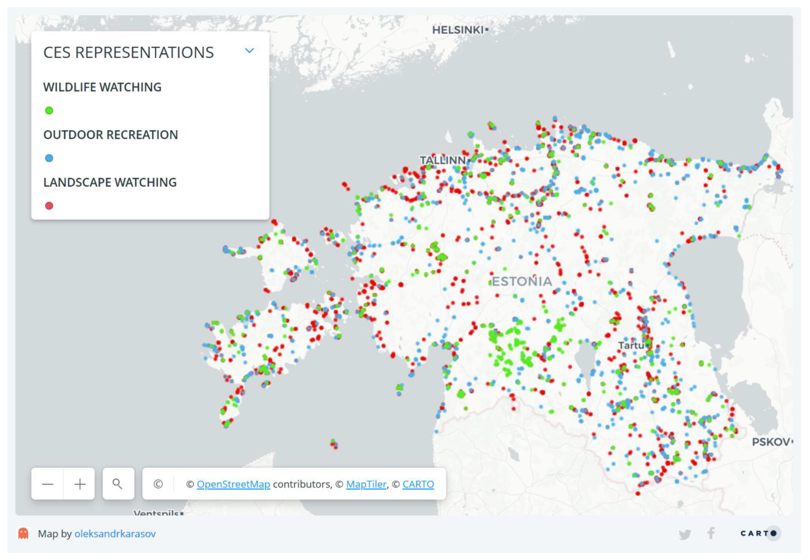
- Landscape watching. This consists of the following tags: nature, outdoors, landscape, tree, nobody, wood, sky, travel, water, and summer (6154 photographs; 17 manually transferred from topic 3).
- Active outdoor recreation. This consists of the following tags: people, recreation, adult, fun, man, leisure, outdoors, one, sport, and action (2345 photographs; 770 manually transferred from topic 1, and 114 from topic 3).
- Wildlife watching. This consists of the following tags: nature, outdoors, no one, flora, leaf, wild, wildlife, season, animal, growth (1484 photographs; 124 manually transferred from topic 1, and 2 from topic 2).
2.3. Impact of Landscape Organisation on CES Use
3. Results
3.1. Mapping of CES Represented in Social Media in Estonia
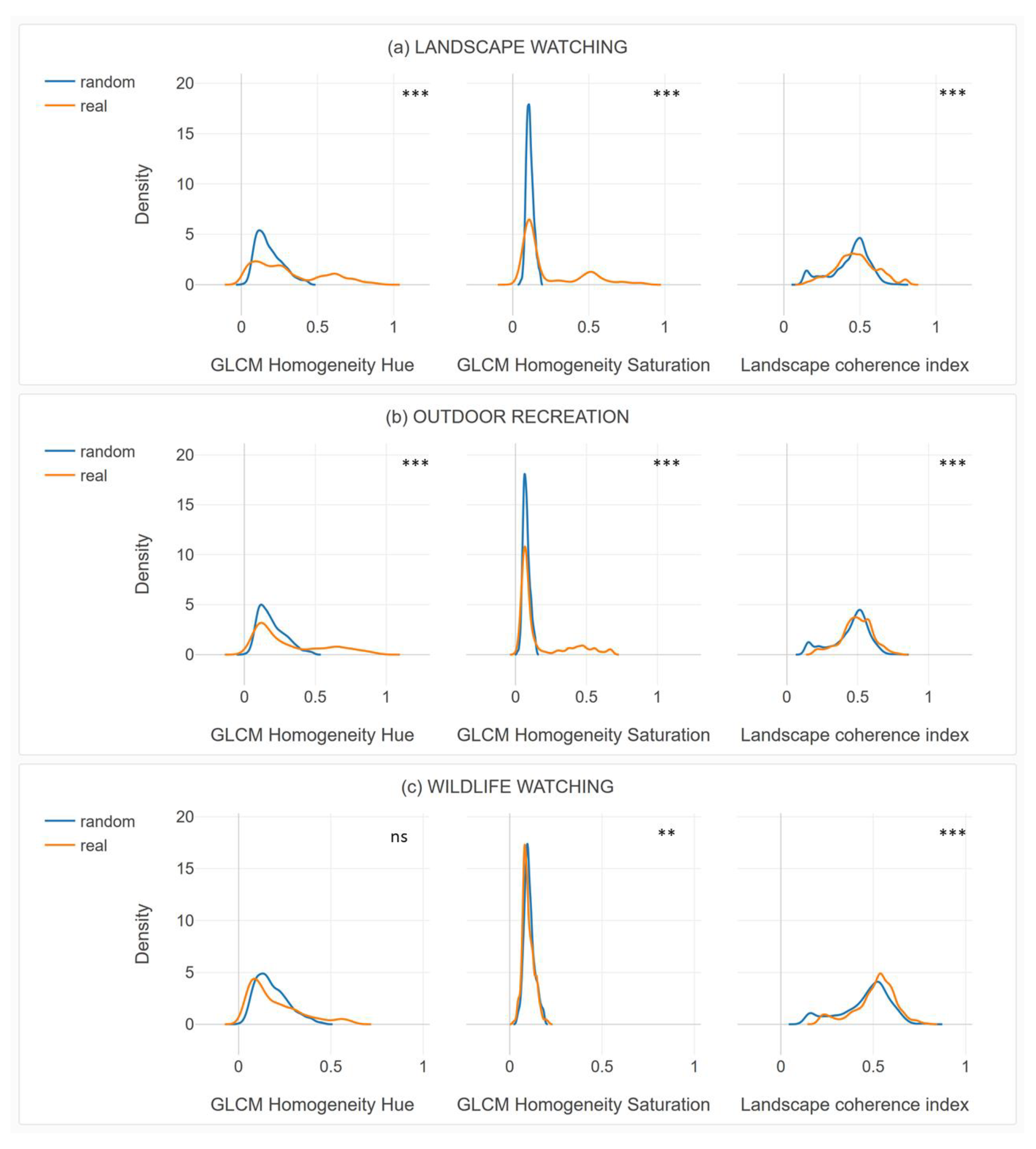
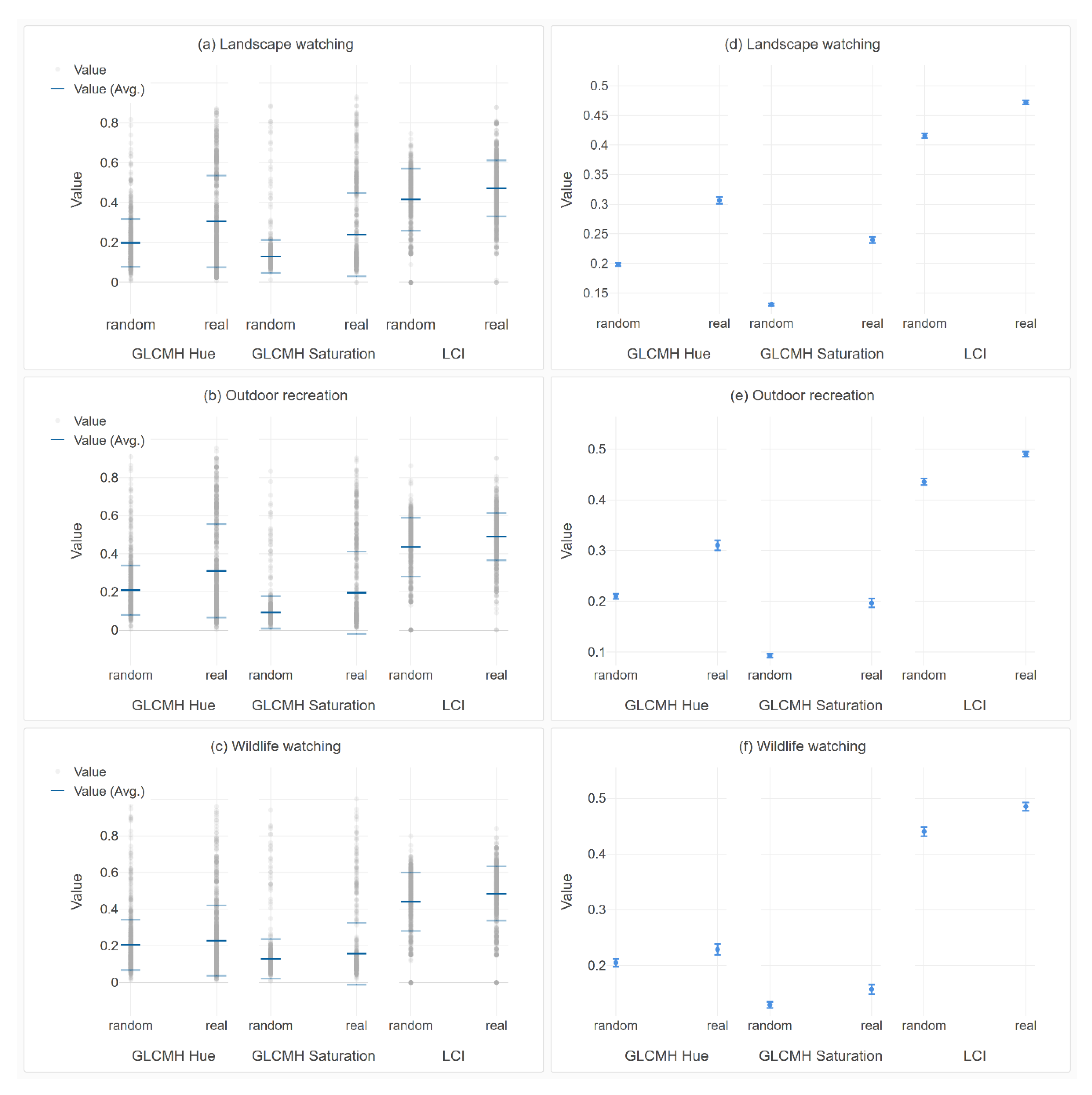
3.2. Impact of Landscape Organisation on CES Use
4. Discussion
4.1. Mapping of CES Represented in Social Media in Estonia
4.2. Impact of Landscape Organisation on CES Use
4.3. Other Sources of Bias
5. Conclusions
Supplementary Materials
Author Contributions
Funding
Acknowledgments
Conflicts of Interest
Appendix A

| Indicator | U Statistic | p Value | Difference | Conf High | Conf Low |
|---|---|---|---|---|---|
| Landscape watching | |||||
| GLCM homogeneity hue | 14,795,531.5 | 9.88 × 10−98 | −0.061 | −0.055 | −0.068 |
| GLCM homogeneity saturation | 14,594,742.5 | 2.91 × 10−107 | 0.017 | −0.015 | −0.018 |
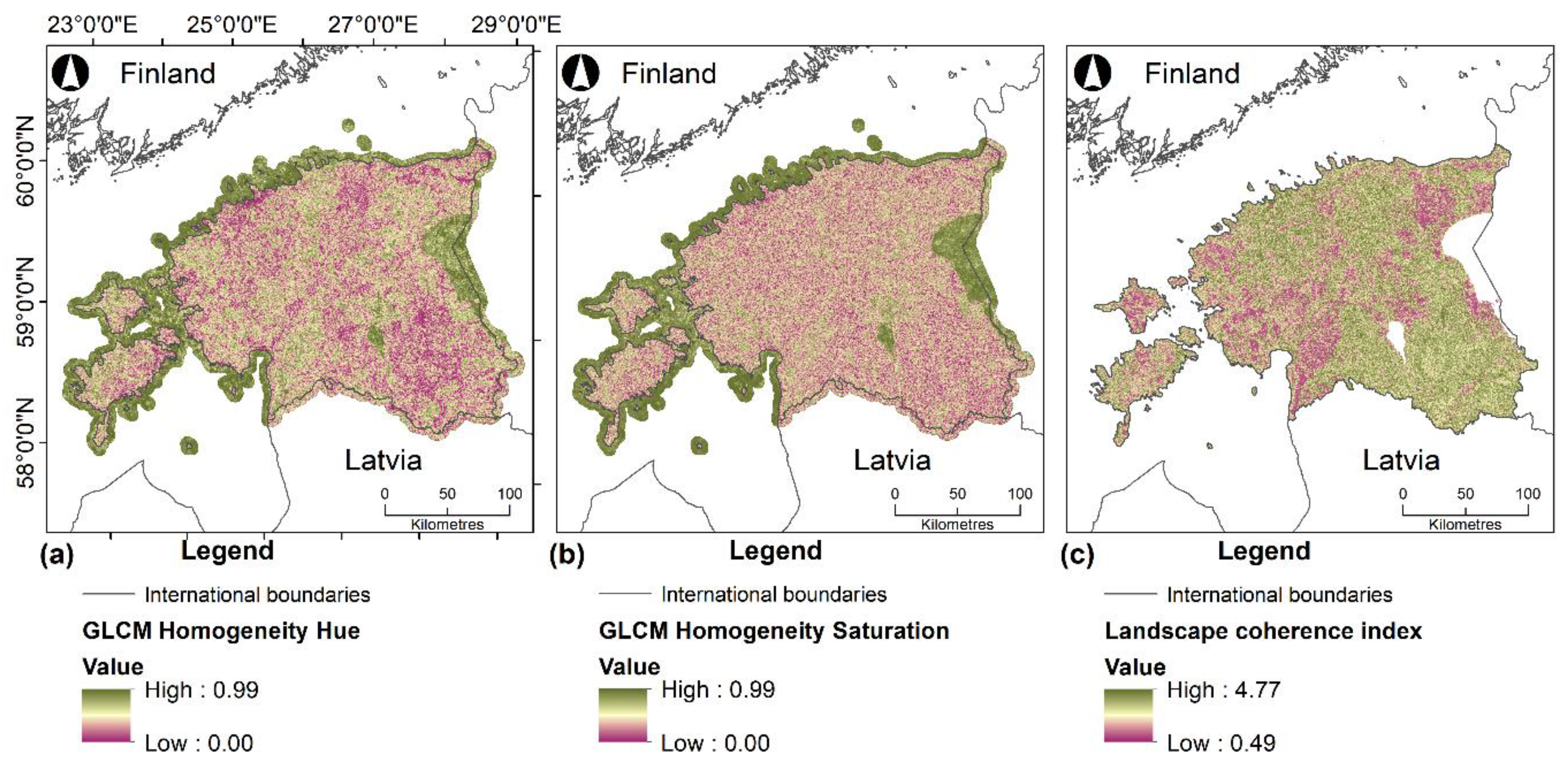
| Landscape coherence index | 16,273,215.5 | 2.01 × 10−41 | −0.033 | −0.029 | −0.039 |
| Outdoor recreation | |||||
| GLCM homogeneity hue | 2,356,245 | 2.21 × 10⁻¹⁷ | −0.032 | −0.024 | −0.040 |
| GLCM homogeneity saturation | 2,293,880 | 8.59 × 10⁻²³ | −0.011 | −0.008 | −0.013 |
| Landscape coherence index | 2,280,950.5 | 5.18 × 10⁻²⁴ | −0.035 | −0.029 | −0.042 |
| Wildlife watching | |||||
| GLCM homogeneity hue | 1,140,081 | 0.095 | 0.007 | 0.015 | −0.001 |
| GLCM homogeneity saturation | 1,168,362 | 0.004 | 0.004 | 0.006 | 0.001 |
| Landscape coherence index | 898,071.5 | 3.34 × 10⁻¹⁸ | −0.037 | −0.029 | −0.046 |
| Indicator | Type | Number of Rows | Mean | Confidence Low | Confidence High | Standard Error of Mean | Standard Deviation | Minimum | Maximum |
|---|---|---|---|---|---|---|---|---|---|
| Landscape watching | |||||||||
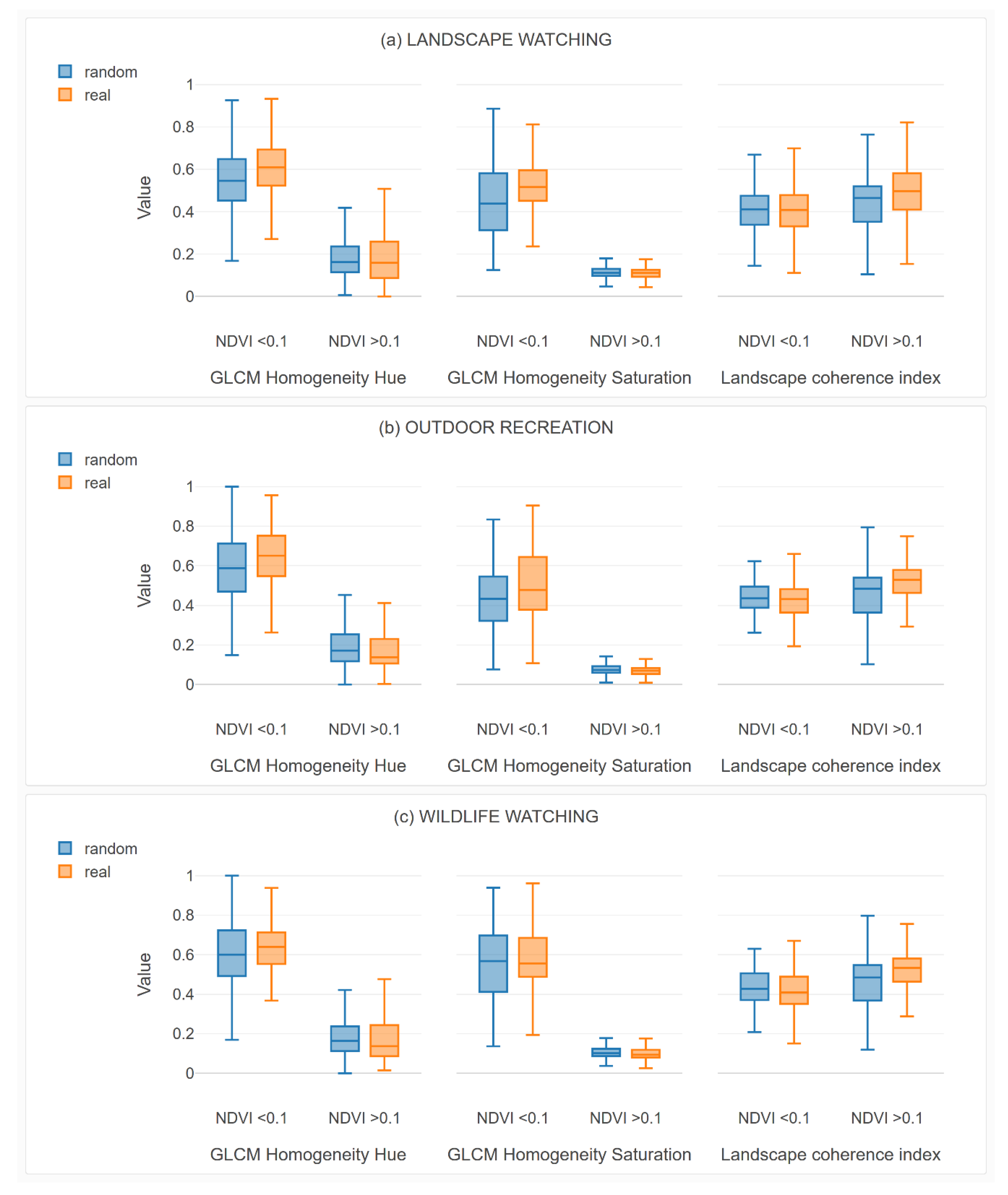
| GLCM homogeneity hue | random | 6153 | 0.20 | 0.20 | 0.20 | 0.00 | 0.12 | 0.01 | 1.00 |
| GLCM homogeneity hue | real | 6153 | 0.31 | 0.30 | 0.31 | 0.00 | 0.23 | 0.00 | 0.93 |
| GLCM homogeneity saturation | random | 6153 | 0.13 | 0.13 | 0.13 | 0.00 | 0.08 | 0.01 | 1.00 |
| GLCM homogeneity saturation | real | 6153 | 0.24 | 0.24 | 0.24 | 0.00 | 0.21 | 0.00 | 0.93 |
| Landscape coherence index | random | 6153 | 0.42 | 0.41 | 0.42 | 0.00 | 0.16 | 0.00 | 0.87 |
| Landscape coherence index | real | 6153 | 0.47 | 0.47 | 0.48 | 0.00 | 0.14 | 0.00 | 1.00 |
| Outdoor recreation | |||||||||
| GLCM homogeneity hue | random | 2345 | 0.21 | 0.21 | 0.21 | 0.00 | 0.13 | 0.00 | 1,00 |
| GLCM homogeneity hue | real | 2345 | 0.31 | 0.30 | 0.32 | 0.01 | 0.25 | 0.00 | 0.96 |
| GLCM homogeneity saturation | random | 2345 | 0.09 | 0.09 | 0.10 | 0.00 | 0.09 | 0.00 | 1.00 |
| GLCM homogeneity saturation | real | 2345 | 0.20 | 0.19 | 0.20 | 0.00 | 0.22 | 0.01 | 0.90 |
| Landscape coherence index | random | 2345 | 0.44 | 0.43 | 0.44 | 0.00 | 0.15 | 0.00 | 0.87 |
| Landscape coherence index | real | 2345 | 0.49 | 0.49 | 0.49 | 0.00 | 0.12 | 0.00 | 1.00 |
| Wildlife watching | |||||||||
| GLCM homogeneity hue | random | 1484 | 0.20 | 0.20 | 0.21 | 0.00 | 0.14 | 0.00 | 1.00 |
| GLCM homogeneity hue | real | 1484 | 0.23 | 0.22 | 0.24 | 0.00 | 0.19 | 0.01 | 0.96 |
| GLCM homogeneity saturation | random | 1484 | 0.13 | 0.12 | 0.13 | 0.00 | 0.11 | 0.01 | 0.94 |
| GLCM homogeneity saturation | real | 1484 | 0.16 | 0.15 | 0.16 | 0.00 | 0.17 | 0.00 | 1.00 |
| Landscape coherence index | random | 1484 | 0.44 | 0.43 | 0.45 | 0.00 | 0.16 | 0.00 | 0.80 |
| Landscape coherence index | real | 1484 | 0.48 | 0.48 | 0.49 | 0.00 | 0.15 | 0.00 | 1.00 |

References
- Saint-Marc, P. The Socialization of the Environment; Stock: Paris, France, 1971. [Google Scholar]
- Costanza, R.; D’Arge, R.; De Groot, R.; Farber, S.; Grasso, M.; Hannon, B.; Limburg, K.; Naeem, S.; O’Neill, R.V.; Paruelo, J.; et al. The value of the world’s ecosystem services and natural capital. Nature 1997, 387, 253–260. [Google Scholar] [CrossRef]
- Finlayson, M.; Cruz, R.D.; Davidson, N.; Alder, J.; Cork, S.; de Groot, R.S.; Lévêque, C.; Milton, G.R.; Peterson, G.; Pritchard, D.; et al. Millennium Ecosystem Assessment: Ecosystems and Human Well-Being: Wetlands and Water Synthesis; Island Press: Washington, DC, USA, 2005. [Google Scholar]
- Potschin, M.B.; Haines-Young, R.H. Ecosystem services: Exploring a geographical perspective. Prog. Phys. Geogr. 2011, 35, 575–594. [Google Scholar] [CrossRef]
- Wu, J. Landscape sustainability science: Ecosystem services and human well-being in changing landscapes. Landsc. Ecol. 2013, 28, 999–1023. [Google Scholar] [CrossRef]
- Musacchio, L.R. Key concepts and research priorities for landscape sustainability. Landsc. Ecol. 2013, 28, 995–998. [Google Scholar] [CrossRef] [Green Version]
- Plieninger, T.; Bieling, C.; Fagerholm, N.; Byg, A.; Hartel, T.; Hurley, P.; López-Santiago, C.A.; Nagabhatla, N.; Oteros-Rozas, E.; Raymond, C.M.; et al. The Role of Cultural Ecosystem Services in Landscape Management and Planning; Elsevier: Amsterdam, The Netherlands, 2015; Volume 14, pp. 28–33. [Google Scholar]
- Milcu, A.I.; Hanspach, J.; Abson, D.; Fischer, J. Cultural Ecosystem Services: A Literature Review and Prospects for Future Research. Ecol. Soc. 2013, 18, art44. [Google Scholar] [CrossRef] [Green Version]
- Dickinson, D.C.; Hobbs, R.J. Cultural ecosystem services: Characteristics, challenges and lessons for urban green space research. Ecosyst. Serv. 2017, 25, 179–194. [Google Scholar] [CrossRef]
- Tew, E.R.; Simmons, B.I.; Sutherland, W.J. Quantifying cultural ecosystem services: Disentangling the effects of management from landscape features. People Nat. 2019, 1, 70–86. [Google Scholar] [CrossRef] [Green Version]
- Kopperoinen, L.; Luque, S.; Tenerelli, P.; Zulian, G.; Viinikka, A. 5.5. 3. Mapping cultural ecosystem services. Mapp. Ecosyst. Serv. 2017, 197–209. [Google Scholar]
- Figueroa-Alfaro, R.W.; Tang, Z. Evaluating the aesthetic value of cultural ecosystem services by mapping geo-tagged photographs from social media data on Panoramio and Flickr. J. Environ. Plan. Manag. 2017, 60, 266–281. [Google Scholar] [CrossRef]
- Díaz, S.; Demissew, S.; Carabias, J.; Joly, C.; Lonsdale, M.; Ash, N.; Larigauderie, A.; Adhikari, J.R.; Arico, S.; Báldi, A.; et al. The IPBES Conceptual Framework—Connecting nature and people. Curr. Opin. Environ. Sustain. 2015, 14, 1–16. [Google Scholar] [CrossRef] [Green Version]
- Pascual, U.; Balvanera, P.; Díaz, S.; Pataki, G.; Roth, E.; Stenseke, M.; Watson, R.T.; Başak Dessane, E.; Islar, M.; Kelemen, E.; et al. Valuing nature’s contributions to people: The IPBES approach. Curr. Opin. Environ. Sustain. 2017, 26, 7–16. [Google Scholar] [CrossRef] [Green Version]
- Martín-López, B.; Barton, D.N.; Gomez-Baggethun, E.; Boeraeve, F.; McGrath, F.L.; Vierikko, K.; Geneletti, D.; Sevecke, K.J.J.; Pipart, N.; Primmer, E.; et al. A new valuation school: Integrating diverse values of nature in resource and land use decisions. Ecosyst. Serv. 2016, 22, 213–220. [Google Scholar]
- Calcagni, F.; Amorim Maia, A.T.; Connolly, J.J.T.; Langemeyer, J. Digital co-construction of relational values: Understanding the role of social media for sustainability. Sustain. Sci. 2019, 14, 1309–1321. [Google Scholar] [CrossRef]
- Haines-Young, R.; Potschin, M.B. Common International Classification of Ecosystem Services (CICES) V5. 1 and Guidance on the Application of The revised Structure; Fabis Consult. Ltd.: Nottingham, UK, 2018; Volume 53. [Google Scholar]
- Dunford, R.; Harrison, P.; Smith, A.; Dick, J.; Barton, D.N.; Martin-Lopez, B.; Kelemen, E.; Jacobs, S.; Saarikoski, H.; Turkelboom, F.; et al. Integrating methods for ecosystem service assessment: Experiences from real world situations. Ecosyst. Serv. 2018, 29, 499–514. [Google Scholar] [CrossRef]
- La Rosa, D.; Spyra, M.; Inostroza, L.; Rosa, D.L.; Spyra, M.; Inostroza, L. Indicators of Cultural Ecosystem Services for Urban Planning: A Review; Elsevier B.V.: Amsterdam, The Netherlands, 2016; Volume 61, pp. 74–89. [Google Scholar]
- Bachi, L.; Ribeiro, S.C.; Hermes, J.; Saadi, A. Cultural Ecosystem Services (CES) in landscapes with a tourist vocation: Mapping and modeling the physical landscape components that bring benefits to people in a mountain tourist destination in southeastern Brazil. Tour. Manag. 2020, 77, 104017. [Google Scholar] [CrossRef]
- Hausmann, A.; Toivonen, T.; Slotow, R.; Tenkanen, H.; Moilanen, A.; Heikinheimo, V.; Di Minin, E. Social Media Data Can Be Used to Understand Tourists’ Preferences for Nature-Based Experiences in Protected Areas. Conserv. Lett. 2018, 11, e12343. [Google Scholar] [CrossRef] [Green Version]
- Wood, S.A.; Guerry, A.D.; Silver, J.M.; Lacayo, M. Using social media to quantify nature-based tourism and recreation. Sci. Rep. 2013, 3, 2976. [Google Scholar] [CrossRef]
- Van Zanten, B.T.; Van Berkel, D.B.; Meentemeyer, R.K.; Smith, J.W.; Tieskens, K.F.; Verburg, P.H. Continental-scale quantification of landscape values using social media data. Proc. Natl. Acad. Sci. USA 2016, 113, 12974–12979. [Google Scholar] [CrossRef] [Green Version]
- Oteros-Rozas, E.; Martín-López, B.; Fagerholm, N.; Bieling, C.; Plieninger, T. Using social media photos to explore the relation between cultural ecosystem services and landscape features across five European sites. Ecol. Indic. 2018, 94, 74–86. [Google Scholar] [CrossRef]
- Langemeyer, J.; Calcagni, F.; Baró, F. Mapping the intangible: Using geolocated social media data to examine landscape aesthetics. Land Use Policy 2018, 77, 542–552. [Google Scholar] [CrossRef]
- Tenerelli, P.; Demšar, U.; Luque, S. Crowdsourcing indicators for cultural ecosystem services: A geographically weighted approach for mountain landscapes. Ecol. Indic. 2016, 64, 237–248. [Google Scholar] [CrossRef] [Green Version]
- Tieskens, K.F.; Van Zanten, B.T.; Schulp, C.J.E.; Verburg, P.H. Aesthetic appreciation of the cultural landscape through social media: An analysis of revealed preference in the Dutch river landscape. Landsc. Urban Plan. 2018, 177, 128–137. [Google Scholar] [CrossRef]
- Sharp, R.; Tallis, H.T.; Ricketts, T.; Guerry, A.D.; Wood, S.A.; Chaplin-Kramer, R.; Nelson, E.; Ennaanay, D.; Wolny, S.; Olwero, N.; et al. InVEST 3.6.0 User’s Guide; Stanford University: Stanford, CA, USA, 2018. [Google Scholar]
- Mancini, F.; Coghill, G.M.; Lusseau, D. Using social media to quantify spatial and temporal dynamics of nature-based recreational activities. PLoS ONE 2018, 13, e0200565. [Google Scholar] [CrossRef] [PubMed] [Green Version]
- Lee, H.; Seo, B.; Koellner, T.; Lautenbach, S. Mapping cultural ecosystem services 2.0—Potential and shortcomings from unlabeled crowd sourced images. Ecol. Indic. 2019, 96, 505–515. [Google Scholar] [CrossRef] [Green Version]
- Richards, D.R.; Tunçer, B. Using image recognition to automate assessment of cultural ecosystem services from social media photographs. Ecosyst. Serv. 2018, 31, 318–325. [Google Scholar] [CrossRef]
- Gosal, A.S.; Geijzendorffer, I.R.; Václavík, T.; Poulin, B.; Ziv, G. Using social media, machine learning and natural language processing to map multiple recreational beneficiaries. Ecosyst. Serv. 2019, 38, 100958. [Google Scholar] [CrossRef] [Green Version]
- Kaplan, R.; Kaplan, S. The Experience of Nature: A Psychological Perspective; Cambridge University Press: Cambridge, UK, 1989; ISBN 0521341396. [Google Scholar]
- Karasov, O.; Vieira, A.A.B.; Külvik, M.; Chervanyov, I. Landscape coherence revisited: GIS-based mapping in relation to scenic values and preferences estimated with geolocated social media data. Ecol. Indic. 2020, 111, 105973. [Google Scholar] [CrossRef]
- Sullivan, R.G.; Meyer, M.E. Environmental Reviews and Case Studies: The National Park Service Visual Resource Inventory: Capturing the Historic and Cultural Values of Scenic Views. Environ. Pract. 2016, 18, 166–179. [Google Scholar] [CrossRef] [Green Version]
- Karasov, O.; Külvik, M.; Chervanyov, I.; Priadka, K. Mapping the extent of land cover colour harmony based on satellite Earth observation data. GeoJournal 2019, 84, 1057–1072. [Google Scholar] [CrossRef]
- Kemp, S. Kepios Team Digital 2019: Estonia. Available online: https://datareportal.com/reports/digital-2019-estonia?rq=estonia (accessed on 29 January 2020).
- Santos-Martin, F.; Viinikka, A.; Mononen, L.; Brander, L.M.; Vihervaara, P.; Liekens, I.; Potschin-Young, M. Creating an operational database for ecosystems services mapping and assessment methods. One Ecosyst. 2018, 3, e26719. [Google Scholar] [CrossRef]
- OpenStreetMap Contributors Planet Dump. Available online: https://planet.openstreetmap.org/ (accessed on 9 April 2020).
- Demšar, J.; Curk, T.; Erjavec, A.; Gorup, Č.; Hočevar, T.; Milutinovič, M.; Možina, M.; Polajnar, M.; Toplak, M.; Starič, A.; et al. Orange: Data mining toolbox in python. J. Mach. Learn. Res. 2013, 14, 2349–2353. [Google Scholar]
- Karasov, O.; Külvik, M.; Burdun, I. Deconstructing landscape pattern: Applications of remote sensing to physiognomic landscape mapping. GeoJournal 2019, 1–27. [Google Scholar] [CrossRef]
- Ou, L.-C.; Yuan, Y.; Sato, T.; Lee, W.-Y.; Szabó, F.; Sueeprasan, S.; Huertas, R. Universal models of colour emotion and colour harmony. Color Res. Appl. 2018, 43, 736–748. [Google Scholar] [CrossRef]
- Haralick, R.M.; Shanmugam, K.; Dinstein, I. Textural Features for Image Classification. IEEE Trans. Syst. Man. Cybern. 1973, 6, 610–621. [Google Scholar] [CrossRef] [Green Version]
- Hall-Beyer, M. GLCM Texture: A Tutorial v. 3.0. Available online: https://0-doi-org.brum.beds.ac.uk/10.13140/rg.2.2.12424.21767 (accessed on 17 May 2020).
- Schloss, K.B.; Palmer, S.E. Aesthetic response to color combinations: Preference, harmony, and similarity. Atten. Percept. Psychophys. 2011, 73, 551–571. [Google Scholar] [CrossRef]
- Antrop, M.; Van Eetvelde, V. Basic Concepts of a Complex Spatial System. In Landscape Perspectives: The Holistic Nature of Landscape; Springer: Dordrecht, The Netherlands, 2017; pp. 81–101. [Google Scholar]
- Lutsenko, E.V. Conceptual principles of the system (emergent) information theory and its application for the cognitive modelling of the active objects (entities). In Proceedings of the IEEE International Conference on Artificial Intelligence Systems, ICAIS, Divnomorskoe, Russia, 5–10 September 2002; Institute of Electrical and Electronics Engineers Inc.: Piscataway, NJ, USA, 2002; pp. 268–269. [Google Scholar]
- Conrad, O.; Bechtel, B.; Bock, M.; Dietrich, H.; Fischer, E.; Gerlitz, L.; Wehberg, J.; Wichmann, V.; Böhner, J. System for Automated Geoscientific Analyses (SAGA) v. 2.1.4. Geosci. Model Dev. 2015, 8, 1991–2007. [Google Scholar] [CrossRef] [Green Version]
- Sahraoui, Y.; Vuidel, G.; Joly, D.; Foltête, J.C. Integrated GIS software for computing landscape visibility metrics. Trans. GIS 2018, 22, 1310–1323. [Google Scholar] [CrossRef]
- Copernicus Land Monitoring Service EU-DEM v1.1—Copernicus Land Monitoring Service. Available online: https://land.copernicus.eu/imagery-in-situ/eu-dem/eu-dem-v1.1?tab=metadata (accessed on 13 September 2018).
- Van Berkel, D.B.; Tabrizian, P.; Dorning, M.A.; Smart, L.; Newcomb, D.; Mehaffey, M.; Neale, A.; Meentemeyer, R.K. Quantifying the visual-sensory landscape qualities that contribute to cultural ecosystem services using social media and LiDAR. Ecosyst. Serv. 2018, 31, 326–335. [Google Scholar] [CrossRef]
- Ghermandi, A.; Sinclair, M. Passive crowdsourcing of social media in environmental research: A systematic map. Glob. Environ. Chang. 2019, 55, 36–47. [Google Scholar] [CrossRef]
- Cao, Y.; Wu, Y.; Zhang, Y.; Tian, J. Landscape pattern and sustainability of a 1300-year-old agricultural landscape in subtropical mountain areas, Southwestern China. Int. J. Sustain. Dev. World Ecol. 2013, 20, 349–357. [Google Scholar] [CrossRef]
- Burkhard, B.; Maes, J.; Potschin-Young, M.B.; Santos-Martín, F.; Geneletti, D.; Stoev, P.; Kopperoinen, L.; Adamescu, C.M.; Adem Esmail, B.; Arany, I.; et al. Mapping and assessing ecosystem services in the EU—Lessons learned from the ESMERALDA approach of integration. One Ecosyst. 2018, 3, e29153. [Google Scholar] [CrossRef]
- Kim, Y.; Kim, C.K.; Lee, D.K.; Lee, H.W.; Andrada, R.I.T. Quantifying nature-based tourism in protected areas in developing countries by using social big data. Tour. Manag. 2019, 72, 249–256. [Google Scholar] [CrossRef]
- Tenkanen, H.; Di Minin, E.; Heikinheimo, V.; Hausmann, A.; Herbst, M.; Kajala, L.; Toivonen, T. Instagram, Flickr, or Twitter: Assessing the usability of social media data for visitor monitoring in protected areas. Sci. Rep. 2017, 7, 17615. [Google Scholar] [CrossRef] [PubMed] [Green Version]
- Yoshimura, N.; Hiura, T. Demand and supply of cultural ecosystem services: Use of geotagged photos to map the aesthetic value of landscapes in Hokkaido. Ecosyst. Serv. 2017, 24, 68–78. [Google Scholar] [CrossRef]
- Martínez Pastur, G.; Peri, P.L.; Lencinas, M.V.; García-Llorente, M.; Martín-López, B. Spatial patterns of cultural ecosystem services provision in Southern Patagonia. Landsc. Ecol. 2016, 31, 383–399. [Google Scholar] [CrossRef]
- Statistics Estonia. The Majority of Enterprises use Information and Communication Technology (ICT) security measures—Statistics Estonia. Available online: https://www.stat.ee/news-release-2019-111 (accessed on 7 February 2020).
- Dunkel, A. Visualizing the perceived environment using crowdsourced photo geodata. Landsc. Urban Plan. 2015, 142, 173–186. [Google Scholar] [CrossRef]
- Hermes, J.; Van Berkel, D.; Burkhard, B.; Plieninger, T.; Fagerholm, N.; von Haaren, C.; Albert, C. Assessment and valuation of recreational ecosystem services of landscapes. Ecosyst. Serv. 2018, 31, 289–295. [Google Scholar] [CrossRef]


© 2020 by the authors. Licensee MDPI, Basel, Switzerland. This article is an open access article distributed under the terms and conditions of the Creative Commons Attribution (CC BY) license (http://creativecommons.org/licenses/by/4.0/).
Share and Cite
Karasov, O.; Heremans, S.; Külvik, M.; Domnich, A.; Chervanyov, I. On How Crowdsourced Data and Landscape Organisation Metrics Can Facilitate the Mapping of Cultural Ecosystem Services: An Estonian Case Study. Land 2020, 9, 158. https://0-doi-org.brum.beds.ac.uk/10.3390/land9050158
Karasov O, Heremans S, Külvik M, Domnich A, Chervanyov I. On How Crowdsourced Data and Landscape Organisation Metrics Can Facilitate the Mapping of Cultural Ecosystem Services: An Estonian Case Study. Land. 2020; 9(5):158. https://0-doi-org.brum.beds.ac.uk/10.3390/land9050158
Chicago/Turabian StyleKarasov, Oleksandr, Stien Heremans, Mart Külvik, Artem Domnich, and Igor Chervanyov. 2020. "On How Crowdsourced Data and Landscape Organisation Metrics Can Facilitate the Mapping of Cultural Ecosystem Services: An Estonian Case Study" Land 9, no. 5: 158. https://0-doi-org.brum.beds.ac.uk/10.3390/land9050158