Modelling Transitions in Regimes of Lubrication for Rough Surface Contact


1
UTM Centre for Low Carbon Transport in Cooperation with Imperial College London, Universiti Teknologi Malaysia (UTM), Johor Bahru 81310, Johor, Malaysia
2
School of Mechanical Engineering, Faculty of Engineering, Universiti Teknologi Malaysia (UTM), Johor Bahru 81310, Johor, Malaysia
3
Malaysian Institute of Chemical and Bio-engineering Technology, University Kuala Lumpur Malaysia (UniKL MICET), Alor Gajah 78000, Melaka, Malaysia
4
Biomass Processing Lab, Center of Biofuel and Biochemical Research, Institute of Self-Sustainable Building, Universiti Teknologi PETRONAS, Tronoh 32610, Perak, Malaysia
5
Chemical Engineering Department, Universiti Teknologi PETRONAS, Tronoh 32610, Perak, Malaysia
*
Author to whom correspondence should be addressed.
Lubricants 2019, 7(9), 77; https://0-doi-org.brum.beds.ac.uk/10.3390/lubricants7090077
Submission received: 25 July 2019
/
Revised: 24 August 2019
/
Accepted: 30 August 2019
/
Published: 2 September 2019
(This article belongs to the Special Issue Tribology of Powertrain Systems)
Abstract
:Accurately predicting frictional performance of lubrication systems requires mathematical predictive tools with reliable lubricant shear-related input parameters, which might not be easily accessible. Therefore, the study proposes a semi-empirical framework to predict accurately the friction performance of lubricant systems operating across a wide range of lubricant regimes. The semi-analytical framework integrates laboratory-scale experimental measurements from a pin-on-disk tribometer with a unified numerical iterative scheme. The numerical scheme couples the effect of hydrodynamic pressure generated from the lubricant and interacting asperity pressure, essential along the mixed lubrication regime. The lubricant viscosity-pressure coefficient is determined using a free-volume approach, requiring only the lubricant viscosity-temperature relation as the input. The simulated rough surface contact shows transition in lubricant regimes, from the boundary to the elastohydrodynamic lubrication regime with increasing sliding velocity. Through correlation with pin-on-disk frictional measurements, the slope of the limiting shear stress-pressure relation and the pressure coefficient of boundary shear strength m for the studied engine lubricants are determined. Thus, the proposed approach presents an effective and robust semi-empirical framework to determine shear properties of fully-formulated engine lubricants. These parameters are essential for application in mathematical tools to predict more accurately the frictional performance of lubrication systems operating across a wide range of lubrication regimes.
1. Introduction
Global transportation energy demand from the year 2017 to the year 2050 has been projected to increase by 45.4% [1]. Such a rapid energy demand increase presents a challenge to the transportation sector in mitigating greenhouse gas (GHG) emissions because of its heavy reliance on fossil fuels. For a typical passenger car, a recent study showed that only 17.5% of the total fuel energy available is used to move the vehicle, with 35.7% being lost to friction [2]. Approximately 50.1% of these frictional losses originate from the internal combustion engine. Holmberg et al. suggested that by adopting new advances in the field of tribology, such as using low-viscosity and low-shear lubricants with more effective additives, these frictional losses could be reduced by at least 18% [3].
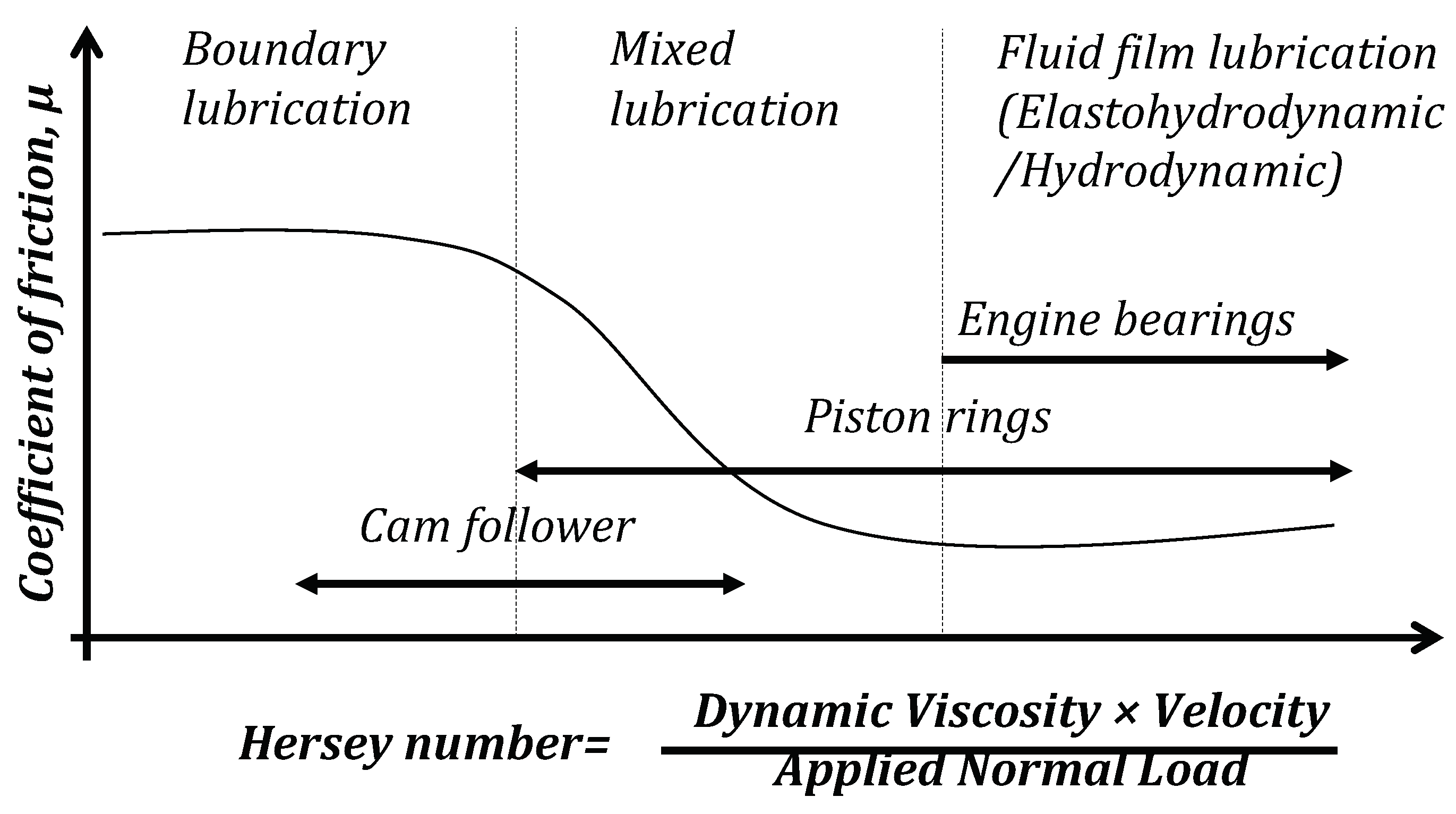
Producing an effective lubricant requires a thorough understanding of the operating lubrication regimes for the intended machine element. In the field of tribology, lubrication regimes are typically depicted using the classical Stribeck curve [4,5]. Figure 1 shows a typical Stribeck curve as a function of the Hersey number. The curve outlines lubrication regimes, namely boundary, mixed, and fluid film lubrication regimes. In an internal combustion engine for a typical passenger car, the same fully-formulated engine lubricant is often used in lubrication systems of major components, such as the cam follower, piston rings, and engine bearings. However, it is also known that these engine components operate at different lubrication regimes, ranging from boundary to fluid film lubrication regimes. Hence, it is imperative that a properly-formulated engine lubricant be capable of operating across a wide range of lubrication regimes.
A fully-experimental approach is often required to ascertain the Stribeck curve for lubricants in determining the transition of lubrication regimes at different operating conditions. Measurements of lubrication regime transitions are usually conducted using friction testers or tribometers. For example, using a ball-on-disk mini traction machine (MTM), LaFountain et al. demonstrated Stribeck-type frictional trends for different lubricant blends [6]. Wang et al. also observed lubrication regime transition from the boundary to the elastohydrodynamic lubrication regime for a point contact using a Universal Material Tester (UMT) [7]. By running a pin-on-disk tribometer, Kovalchenko et al. [8] studied the transitions of lubrication regimes for laser-textured surfaces. Using a newly-developed ball-on-disk tribometer, capable of operating under rolling-sliding conditions for speeds up to 60 m/s, He et al. measured the coefficient of friction variation for base and fully-formulated lubricants, showing transition of lubrication regimes similar to a Stribeck curve [9]. More recently, Stribeck-type lubrication regime transitions for biolubricants, such as fatty acid methyl esters, were also measured using tribometers in order to characterize the tribological performance of such lubricants at different lubrication regimes [10,11].
A more cost-efficient method in observing the transitions of lubrication regimes, similar to a Stribeck curve, is to resort to deriving mathematical tools, reducing the dependency on experimental investigations. A mathematical tool, simulating lubrication regime transitions, should consider the surface roughness effect, which controls the onset of various lubrication regimes, especially the transition point from the mixed to fluid film lubrication regime. One of the approaches is to apply the flow factor method proposed by Patir and Cheng [12]. Their averaged Reynolds solution took into consideration the effect of fluid flow through rough surfaces using flow factors. Such a concept has been widely applied where a mixed lubrication regime is concerned [13,14,15] and also for studies on friction reduction through surface modification/texturing [16,17,18]. However, Venner and Napel pointed out that the flow factors commonly used for most mixed lubrication analysis are still based on Patir and Cheng’s work [12], which was derived from hydrodynamic analysis [19]. More importantly, Venner and Napel also noted that elastic deformation of surface asperities is also not factored in this approach [19]. Hence, to apply this method effectively along a mixed lubrication regime, flow factors must be derived considering non-Newtonian properties of the lubricant flow across rough surfaces together with the deformation of surface asperities.
As an alternative to the flow factor method, Venner and Napel proposed the application of a deterministic approach in simulating tribological conjunctions along mixed lubrication regime [19]. The approach incorporates a measured surface topography along with the Reynolds solution. Applying the deterministic approach, Hu and Dong simulated the whole range of lubrication regime for a tribological contact [20]. Their numerical deterministic solution considered the surface roughness of the contact profile while solving for the Reynolds equation along the fluid film lubrication regime. When fluid film is depleted along the boundary lubrication regime, the Reynolds equation is reduced in the unified solution to consider only the boundary interaction. Zhu et al. further extended this unified numerical solution, considering non-Newtonian properties for typical base lubricants, to simulate the transition of lubrication regimes for counter-formal rough surface contact [21]. Recently, this unified numerical approach was also applied to simulate lubrication regime transitions for a lubricated ball-on-disk contact, comparing well with measured Stribeck curves [9]. However, the accuracy of the deterministic approach still depends heavily on the resolution of the measured surface topography, which has been commonly measured to be random and multi-scale in nature [22].
One could also revert to the load-sharing concept pioneered by Johnson et al. [23] in simulating tribological conjunctions along mixed lubrication. The concept considers the contact load along the tribological conjunction to be the shared between the load generated by the lubricant hydrodynamic pressure and the load carried by interacting surface asperities. Asperity interactions are often integrated using rough surface contact models. For example, Gelinck and Schipper [24] presented a mixed lubrication mathematical model, capable of simulating lubrication regime transitions for a line contact problem based on the load-sharing method. Along mixed and boundary lubrication regimes, where surface asperity interactions become prominent, they applied Greenwood and Williamson’s rough surface contact model [25]. This model was later extended by Popovici and Schipper [26] to simulate lubrication regime transitions for elliptical contact. The load sharing concept was also recently adopted by Zhang et al. [27] and Lijesh and Khonsari [28] for simulating mixed and boundary lubrication problems.
Another mathematical method used to predict friction at different lubrication regimes was given by Teodorescu et al. [29]. The contact pressure, determined by solving for the Reynolds equation, was considered to be shared between: (1) boundary asperity interaction along opposing rough surfaces in relative motion and (2) the hydrodynamic component from entrained lubricant into the conjunction. The load sharing distribution was only decided when determining the frictional forces using Greenwood and Tripp’s rough surface contact model [30]. For this method, the separation parameter (introduced in the classical Stribeck curve [4,5]) and measured topography were used to note that the simulated film thickness, even under ideal conditions (smooth surfaces and fully-flooded inlet) could be insufficient to guard against the interaction of the rough topography of surfaces under certain operating conditions. Thus, the regime of lubrication may be mixed or even boundary. This approach was further extended to investigate tribological properties of a piston ring sliding along an internal combustion engine cylinder liner [31,32] and interacting gear teeth pairs under transient conditions for an automotive transmission system [33]. A further extension of this approach, considering elasto-plastic deformation of surface asperities, was also been reported in the literature [34].
For engine lubrication systems, Taylor pointed out that physical properties of engine lubricant are extremely crucial in predicting the tribological performances of these systems [35]. This requires accurate rheological information of the lubricant, which varies with pressure, temperature, and shear rate, especially along elastohydrodynamic and mixed lubrication regimes. Numerous empirical equations have been derived to describe the dependence of lubricant viscosity on pressure and temperature. One of the earlier ones included the Barus equation [36], which considers lubricant viscosity variation with pressure. Alternatively, Roelands [37] and Appeldorn [38] both derived empirical equations, relating lubricant viscosity to both temperature and pressure. However, citing such empirical approaches to be lacking a theoretical basis, Yasutomi et al. proposed a free volume model, based on a modified Williams, Landel, and Ferry (WLF) equation, to correlate the dependence of lubricant viscosity on temperature and pressure [39]. Wu et al. also proposed a simplistic approach, based on free-volume theory, to predict pressure-viscosity coefficients of typical lubricants (e.g., mineral oils, resin blends, and synthetic hydrocarbons) [40]. The free-volume-based approach has since been further explored to better understand the dependence of viscosity on temperature and pressure [41,42]. Recently, Bair [43] also observed that an alternative method in correlating the dependence of viscosity on pressure and temperature can be used through an indirect method by measuring the elastohydrodynamic film thickness. However, Bair found that the film-derived method lacked the accuracy to represent the piezoviscous behavior of typical lubricants under high pressure conditions sufficiently.
Integrating non-Newtonian lubricant properties, Khonsari and Hua proposed a generalized non-Newtonian Reynolds equation for an elastohydrodynamic line contact problem [44]. Their non-Newtonian model incorporated the rheological model proposed by Bair and Winer [45]. From their study, it was observed that non-Newtonian shear thinning significantly affected the frictional behavior of the lubricant while having minimal effect on the generated contact pressure and film thickness. It is also essential to consider thermal effects for elastohydrodynamic lubrication analysis [46]. Therefore, based on their non-Newtonian Reynolds solution [44], Khonsary and Hua extended the model to include thermal effects for the elastohydrodynamic analysis [46]. Numerous studies on elastohydrodynamic lubrication, which include the thermal effect towards lubricant rheological properties, have also been reported in the literature [6,27,47]. It was shown that for lubricants behaving in a non-Newtonian manner, at sufficiently high shear rates, heat generation within the confined film could lead to the gradual decrease of friction forces. However, He et al. added that such a change in friction force could only be evident at higher speeds, possibly above 1 m/s [9]. This is because the heat generation at low speeds is usually insignificant [21].
It has been realized that parameters available in the literature for mathematical predictive tools, describing the shear properties of lubricants at different lubrication regimes, are often only for typical base lubricants. Such information might not be sufficient to predict accurately frictional losses of machine elements lubricated by fully-formulated lubricants. This is because fully-formulated lubricants contain numerous chemical additives (e.g., friction modifier, extreme pressure additives, anti-wear agent, etc.), which are intended to deliver specific lubrication performances. The lack of information on the shear properties of fully-formulated lubricants at different lubrication regimes proves to be a challenge when attempting to predict frictional losses for lubrication systems accurately. The literature survey covered thus far has shown the capability of numerous existing mathematical models at simulating tribological conjunctions at different lubrication regimes, but mostly based on typical base lubricant properties. Therefore, the present study intends to develop a semi-empirical framework, based on laboratory-scale friction testing using a commercially-available pin-on-disk tribometer, to predict accurately the friction performance of lubricant systems operating across a wide range of lubricant regimes. Through correlation with experimental data, essential shear-related simulation parameters could be ascertained, providing a fundamental platform to predict more accurately the frictional performance of lubrication systems.
2. Mathematical Approach
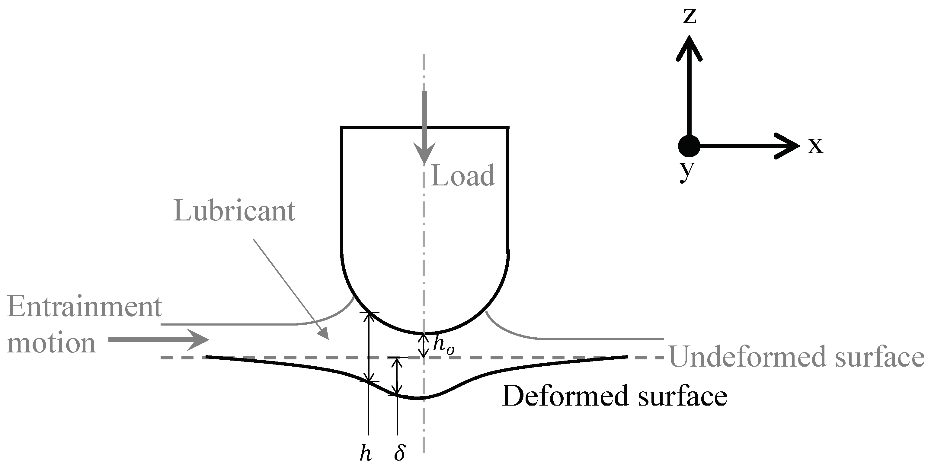
In this study, a mathematical model was derived to determine numerically the frictional properties for a lubricated rough surface point contact under pure sliding as illustrated in Figure 2. Taking into account the pros and cons of various methods reviewed above, the load sharing method was thus selected for the present analysis, where the total contact pressure was assumed to be shared between the lubricant hydrodynamic pressure and the asperity interacting pressure , giving:
The coupling effect of the lubricant hydrodynamic pressure and the asperity interacting pressure was determined by adopting a unified iterative numerical scheme. For the unified solution of the simulated point contact, the elastic film shape of the lubricant h is defined as:
with being defined as the local separation gap at any location within the contact conjunction. The term is given as the minimum clearance between the undeformed opposing surfaces in relative motion (refer to Figure 2).
This equation computes the deflection at a point (), which is determined from all the generated pressures at points (). For a computational grid made with a pressure distribution in a numerical analysis, this equation can be rewritten as:
where the term refers to the influence coefficient for a uniform pressure, acting on a rectangular element with apparent area, () [48]. The term is the effective modulus of elasticity, given as:
Finally, the total contact load can be computed as:
2.1. Hydrodynamic Pressure
The Reynolds equation and the elastic film shape h were simultaneously solved together with lubricant rheological state equations in order to ascertain lubricant fluid film properties (e.g., contact pressure and lubricant film thickness). Assuming that lubricant flow into the contact conjunction is laminar, the tribological behavior of such conjunction can be predicted using a two-dimensional Reynolds equation [50]:
with and referring to the average sliding speed of the contacting surfaces in the x- and y-directions, respectively. For the current study, along the lubricant film rupture point, the Swift–Steiber exit boundary condition [51,52] was applied, where at rupture points in both the x- and y-directions:
Along elastohydrodynamic and mixed lubrication regimes, the lubricant rheology-pressure relation becomes essential. This is because contact pressure generated at these regimes is significantly high to affect the lubricant rheology. Therefore, the current study applied the expression by Dowson and Higginson for lubricant density variation with contact pressure as follows [53]:
For this study, the lubricant viscosity-pressure variation was introduced to the mathematical solution using [40]:
where is known as the lubricant viscosity-pressure coefficient, derived based on a free-volume approach. Procedures involved in determining this coefficient for the selected engine lubricants will be discussed later in the study.
2.2. Interacting Asperity Pressure
When the lubricant film is sufficiently thick, the surface roughness effect becomes negligible. However, even under fully-flooded conditions, the lubricant film could still be insufficient to guard against the interaction of the rough topography of surfaces, leading to mixed or even boundary regimes of lubrication. In the present study, Greenwood and Tripp’s rough surface contact model was used to determine the extent of asperity interactions [30]. The pressure carried by the interacting asperity contact is calculated using [54]:
with the separation parameter given as . The statistical functions, and , are computed using [30]:
In the present study, the solutions for function is computed numerically and then fitted based on the following polynomial expression [31]:
2.3. Frictional Conjunction
Friction generated during sliding of lubricated contact along mixed and boundary regimes of lubrication should take into account viscous and boundary shear components. In this study, the friction model, integrating Greenwood and Tripp’s rough surface contact assumption for a lubricated conjunction, as proposed by Teodorescu et al. [54], was applied. The total shear stress is computed as:
For Newtonian fluid, the viscous shear component is described as follows:
where the lubricant viscosity is calculated using Equation (9). In this study, viscous shearing of non-Newtonian fluid was determined using the limiting shear stress assumption. When the viscous shear stress is larger than the Eyring stress, , non-Newtonian behavior prevails. Hence, is calculated using:
where is the slope of limiting shear stress-pressure relation. Finally, the boundary shear component can be expressed as:
where m is the pressure coefficient of the lubricant boundary shear strength. Thus, the total friction along the rough surface point contact can be determined using:
2.4. Numerical Method
In this study, to compute the hydrodynamic pressure, the Reynolds equation given in Equation (7) is discretized using the notations provided in Appendix A, giving:
where and . The term, S () is known as the squeeze term. For the present analysis, Equation (17) is solved using the finite difference scheme proposed by Jalali-Vahid et al. [55]. Aside from engine tribology-related applications, the scheme has also been adopted to analyze tribological performances of pharmaceutical elastomeric seals [56]. The finite difference scheme is further described in Appendix B. It is noted that a grid size of 120 points × 120 points, for a simulated domain of 0.6 mm × 0.6 mm, was used for the current simulation. This was decided based on the criterion, where the minimum film thickness variation with the grid size and simulation domain was be less than 1% across all the simulated operating conditions.
The current analysis then solved for the elastic film shape based on the coupling effect of hydrodynamic pressure and interacting asperity pressure using a unified iterative numerical scheme. The numerically-converged total contact pressure and elastic film shape were then used to ascertain the frictional properties along the lubricated point contact. It is noted that the model requires two essential lubricant-dependent parameters, which are: (1) the slope of the limiting shear stress-pressure relation and (2) the pressure coefficient of the boundary shear strength m. These values are not readily available for the selected engine lubricants. Therefore, as an initial approximation, these parameters were calibrated iteratively in order to obtain good correlation between the simulated and the measured coefficient of friction. It is also noted that the contact pressure generated by the simulated conditions was observed to be large enough to deem the Eyring stress negligible in the calculations [57,58]. Hence, for all the tested engine lubricants, as a first approximation, the Eyring stress was taken to be 2 MPa [31,59].
3. Experimental Approach
3.1. Friction Testing
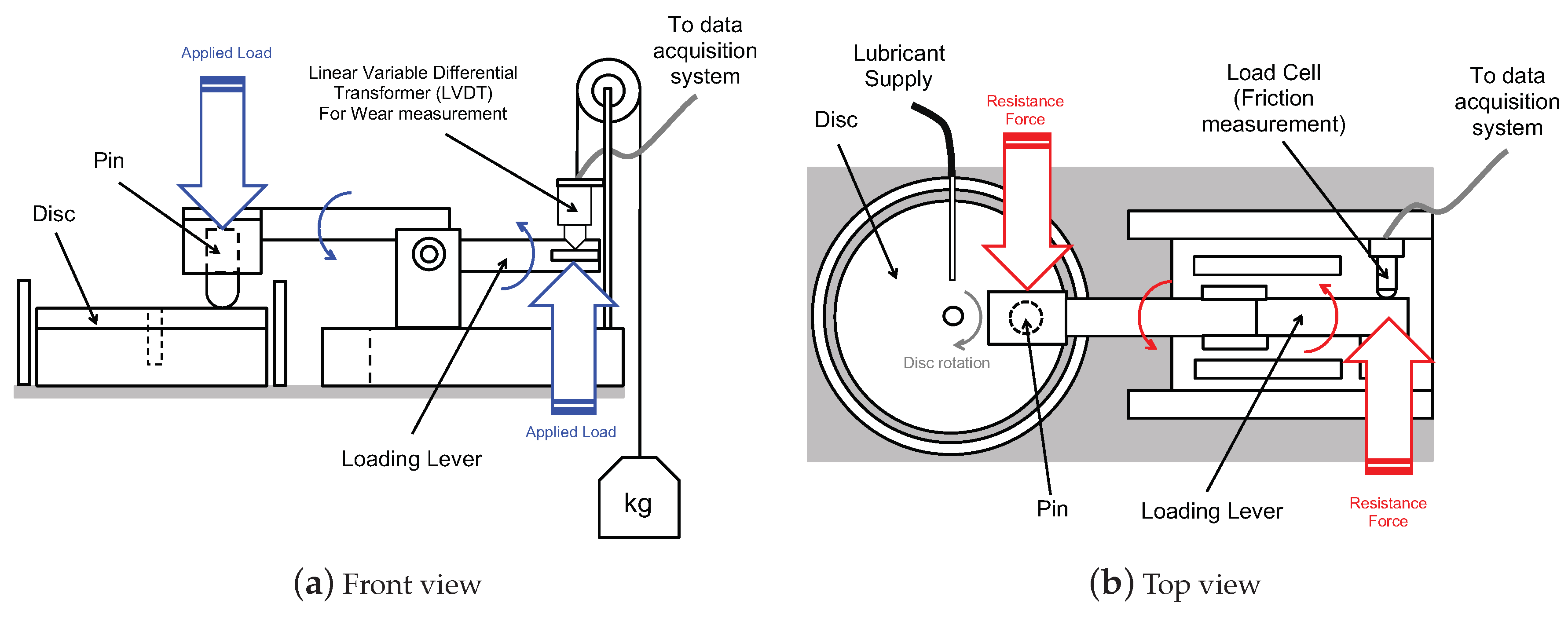
Friction tests were carried out for commercially-available engine lubricants, namely SAE15W40- (mineral oil), SAE10W40- (semi-synthetic), and SAE5W40-grade (fully synthetic) engine lubricants. The measured coefficient of friction values were compared to the ones obtained from the simulated point contact. The test is performed using TE-165 pin-on-disk tribometer (given in Figure 3), manufactured by Magnum Engineers in compliance with ASTM G99. For the present study, a volume of 1.2 liters was prepared for each of the tested lubricants. The disks and stationary pins were fabricated from JISSKD-11 tool steel and cast iron (measured hardness of 87 HRBwith a chemical composition of 3.51% carbon, 3.2% silicon, 0.4% manganese, 0.018% phosphorus, and 0.01% sulfur with the remainder being iron), respectively. The pins were also fabricated to have a spherical end cap with a 5-mm curvature radius. A new set of pins and disks was used for each of the tested engine lubricants. In an attempt to reduce variation caused by using a new set of pins and disks, during fabrication, it was ensured that all pins and disks used for the friction tests had near consistent surface finishings. The parameters with relation to the rough surface characteristics for the pins and the disks was measured using the Taicaan laser profilometer as described by Jackson and Green [60]. The measured parameters are averaged and tabulated in Table 1.
Before being dried in a desiccator, the disks and the stationary pins were cleaned with an ultrasonic cleaner (acetone was used as the cleaning solution) to remove tooling fluid residuals from the machining processes. During the tests, the pin-disk conjunction was subjected to a disk rotational speed between 60 rpm and 2000 rpm with a 20-N applied normal load (approximately 0.96 GPa of nominal maximum Hertzian pressure). This corresponded to disk linear velocity between 0.125 m/s and 4 m/s in which the wear track was fixed at 20 mm from the center of the disk. The friction measurement was then initiated at a 60-rpm disk rotational speed before being increased in a stepwise manner after three and a half minutes of each rotational speed until 2000 rpm. The prescribed procedure enabled the contact to transit from the boundary to mixed and then to the fluid film lubrication regime. These tests were repeated twice for each of the investigated lubricants.
It is noted that during the friction test, lubricant was continuously supplied through a pump. This was to ensure that a fully-flooded lubrication condition was maintained throughout the test duration. However, it was observed that heat was generated as a result of the pumping action. Therefore, a thermocouple was placed at the outlet of the lubricant supply from the pump to measure the initial lubricant temperature before it was entrained into the pin-disk conjunction. The measured lubricant temperature at the supply outlet for the selected SAE-grade engine lubricants is summarized in Appendix D. In order to have a like-for-like simulation-experiment comparison, these temperature values were used to determine the lubricant bulk rheological properties for the simulated point contact.
3.2. Lubricant Viscosity-Pressure Correlation
For the current analysis, the lubricant viscosity-pressure coefficient given in Equation (9) was determined using the free-volume theory proposed by Wu et al. [40]. For mineral oils and synthetic hydrocarbons, Wu et al. suggested that the lubricant viscosity-pressure coefficient be determined using the following expression [40]:
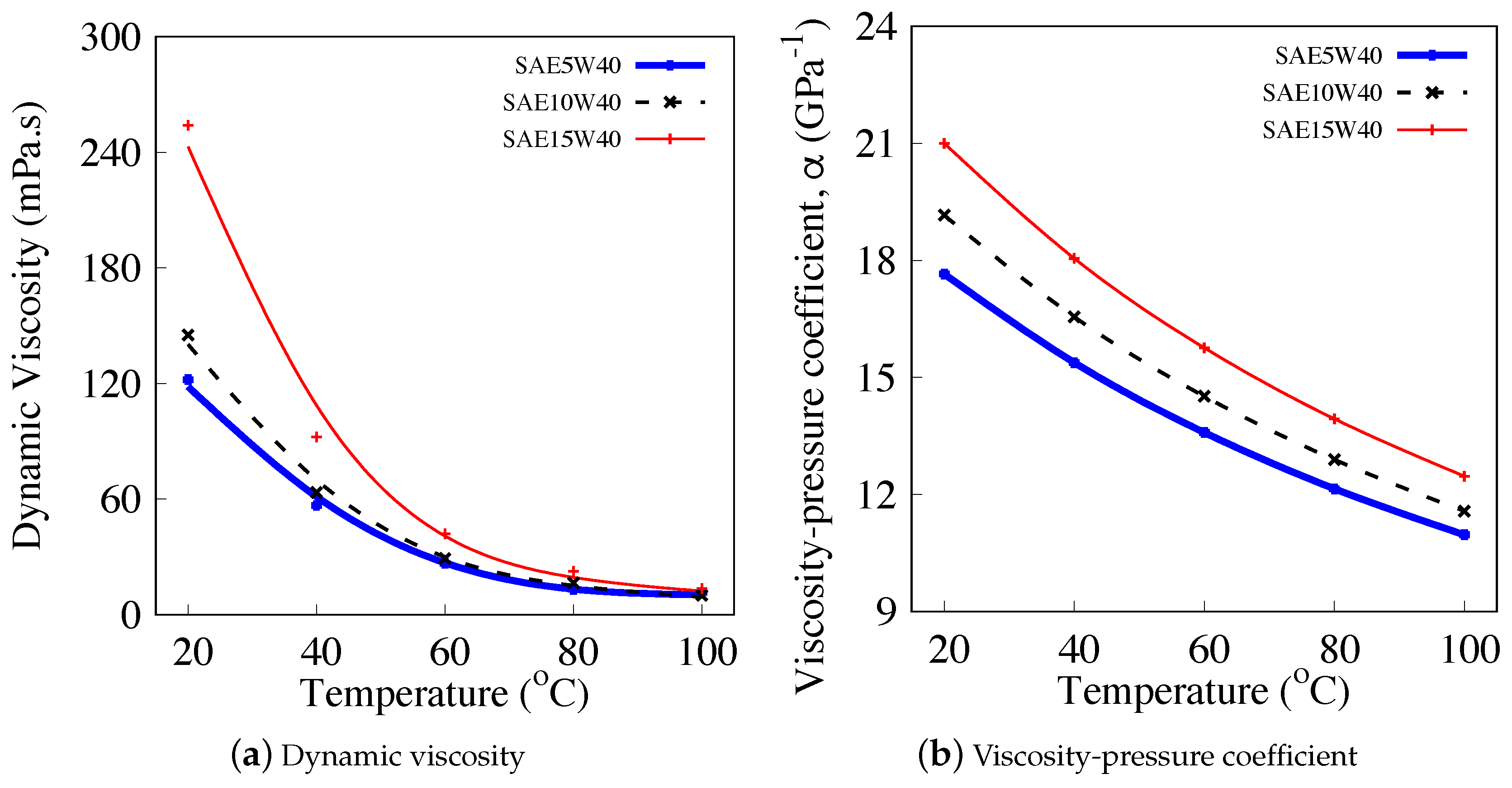
where with T being the lubricant temperature. The terms and are taken as the slope and the interception of the logarithmic linear relationship between the lubricant dynamic viscosity and temperature.
The free-volume-based method requires the lubricant viscosity-temperature relation as the input. Figure 4a shows the lubricant dynamic viscosity measured at different temperatures for the selected engine lubricants using a Bohlin Gemini HR Nano rotational rheometer. During the measurements, a parallel plate of 40 mm in diameter was used to shear the lubricant sample at a 10-s shear rate for temperatures ranging from 20 °C–100 °C. Error bars, representing the standard deviation, are not included in Figure 4a because the standard deviations of the measured viscosity for the tested lubricants were relatively small (less than 3% of the average value). From the lubricant dynamic viscosity-temperature relation, the lubricant viscosity-pressure coefficient, , was calculated at the measured temperature values using Equation (18). The variation of with respect to lubricant temperature is as illustrated in Figure 4b.
4. Results and Discussion
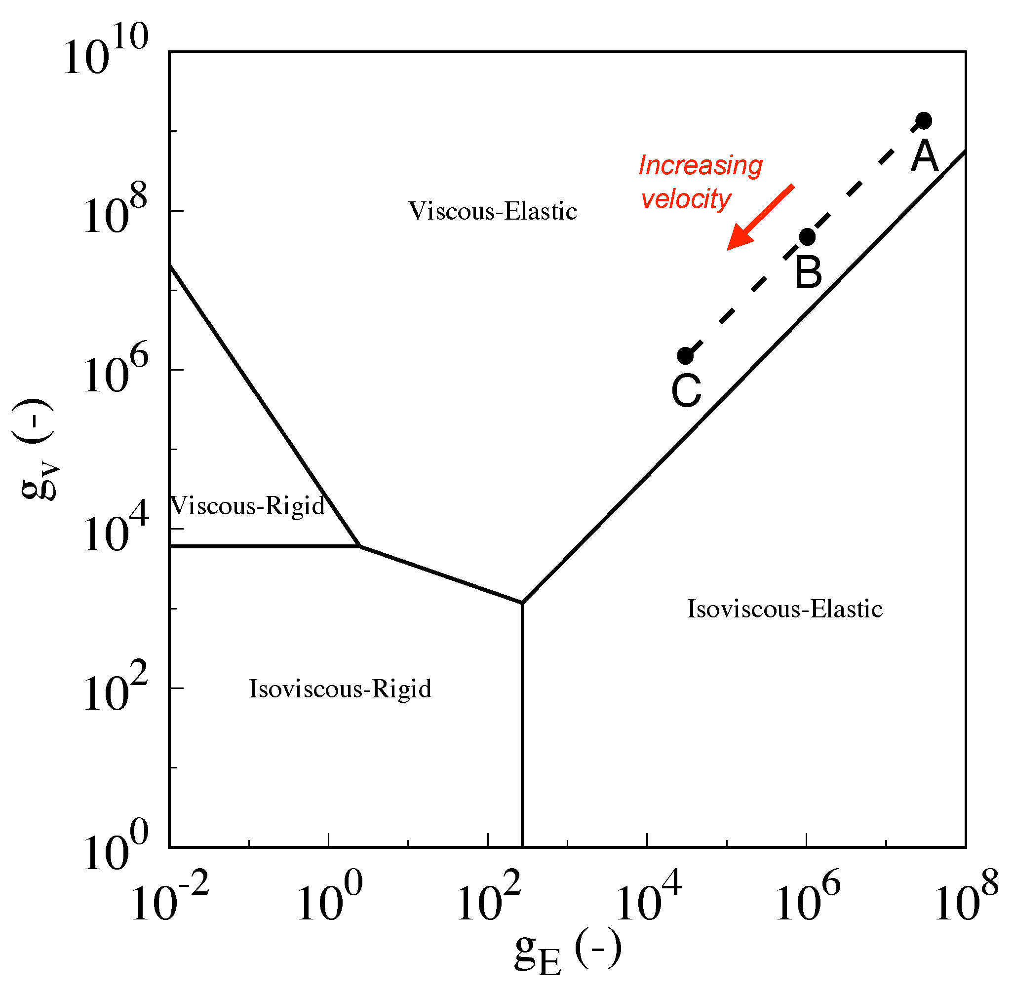
For the current analysis, a lubricated point contact subjected to pure sliding, representing a pin-on-disk tribometer conjunction, was simulated. The predicted frictional properties for the selected engine lubricants were then compared to the ones measured using a pin-on-disk tribometer. To elucidate the nature of the investigated tribological conjunction, lubricated contact conditions were first plotted onto a lubrication regime map as proposed by Esfahanian and Hamrock for a point contact problem [61]. The lubrication regime map required two parameters, namely: (1) the non-dimensional viscosity parameter (= ) and (2) the non-dimensional elasticity parameter (= ). The terms , , and are the non-dimensional load parameter (= ), the non-dimensional speed parameter (= ), and the non-dimensional materials parameter (= ), respectively. From the map given in Figure 5, the operating lubrication regime for SAE10W40-grade engine lubricant was shown to be viscous-elastic, indicating the significance of contact deformation relative to the lubricant film thickness. As the sliding velocity increased, it can be seen that the investigated contact became less viscous-elastic, heading towards the regime of isoviscous-rigid. The observed behavior was believed to be aided by the increased amount of lubricant being entrained into the contact at higher sliding velocities, forming a thicker fluid film that could eventually lead to a hydrodynamic lubrication regime.
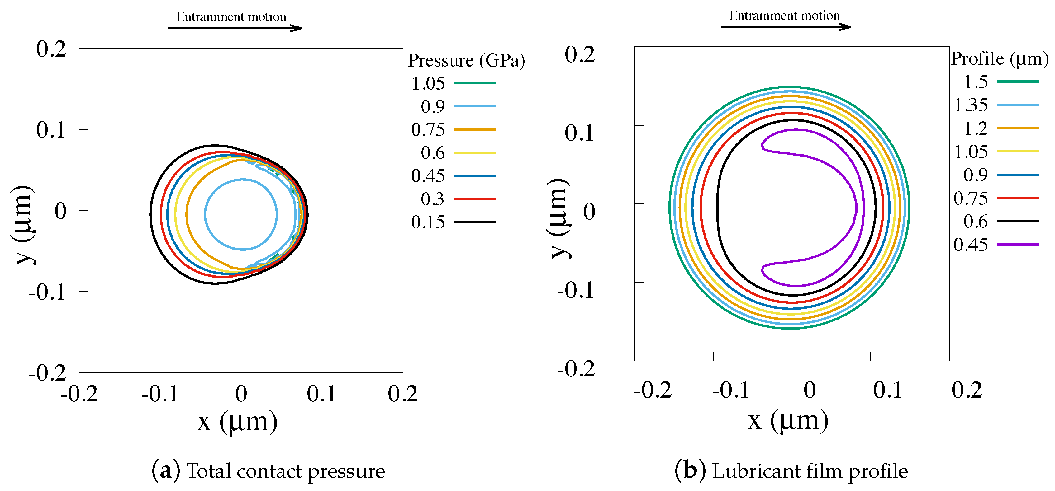
Along the viscous-elastic regime given in Figure 5, contact pressure was expected to be significantly high to increase the lubricant viscosity within the conjunction. Therefore, the lubricant viscosity-pressure relation was deemed to play a significant role in affecting contact pressure and lubricant film formation of the simulated contact. In the current analysis, lubricant properties, namely bulk viscosity and viscosity-pressure coefficient (given in Figure 4), for SAE10W40-grade engine lubricant at a measured lubricant supply temperature of 30 °C, were used to simulate the pin-on-disk conjunction more accurately. The mathematical solution derived for a point contact was utilized to solve iteratively for the lubricated point contact properties (total contact pressure and lubricant elastic film shape). Figure 6a gives the contour of total contact pressure generated from the simulated point contact, lubricated with SAE10W40-grade engine lubricant at a sliding velocity of 4 m/s and applied normal load of 20 N (Location C in Figure 5). The simulated contours correlated well with those observed in [62]. At such operating condition, the contact pressure was shown to be in the range of GPa. Besides this, a horse-shoe-shaped lubricant film constriction can also be observed towards the trailing edge of the point contact, as depicted in Figure 6b. These two characteristics corroborated the operating viscous-elastic regime observed in Figure 5.
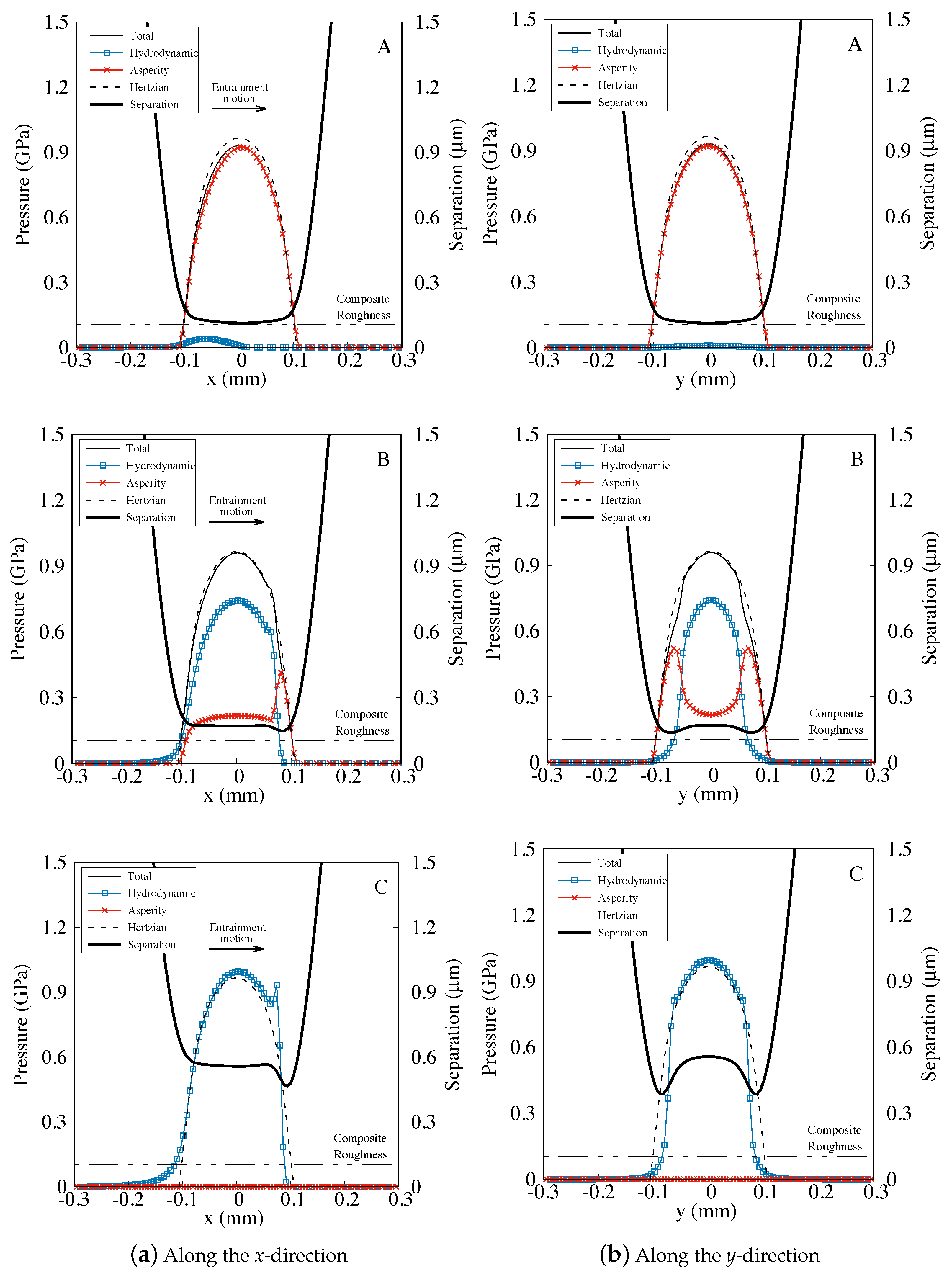
Using the simulation parameters provided in Appendix C, the numerical solution was then applied to further solve for the point contact, lubricated with SAE10W40-grade engine lubricant, at various sliding velocities. Figure 7 shows the central cross-section of the contact pressure and lubricant film profile along the x- and y-directions. At Location A, as denoted in Figure 5, the total contact pressure generated within the conjunction was Hertzian-like, dominated by the interacting asperity pressure. The predicted elastic film shape was also shown to be close to the measured composite surface roughness of 0.105 μm, indicating possible boundary or surface asperity interactions. These properties are typical of characteristics along the boundary lubrication regime. As the sliding velocity increased (from Location A to Location B), more lubricant molecules were entrained into the conjunction, which gave rise to a more significant amount of hydrodynamic pressure. The hydrodynamic pressure began to lift the opposing surfaces further, reducing the interacting asperity pressure, during which the lubrication regime transition from the boundary to mixed lubrication regime was observed. A further increase in sliding velocity (to Location C) then lead to the formation of a secondary peak in the hydrodynamic contact pressure near the trailing edge of the contact, with the predicted film shape now well above the composite surface roughness. Such a film shape, coupled with significantly high contact pressure (in GPa range), was evidence of a fully-formed elastohydrodynamic lubrication, which correlated with the expected viscous-elastic behavior depicted in Figure 5. It is also noted that as sliding velocity increased, the contact pressure began to deviate from the Hertzian pressure, showing an increasing hydrodynamic effect along the conjunction.
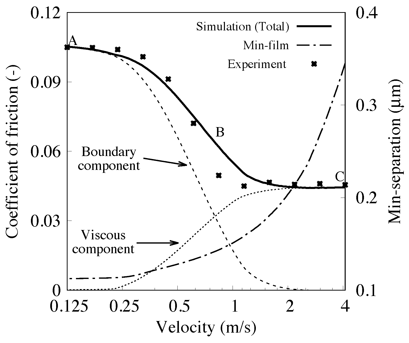
By applying the friction model discussed above, the coefficient of friction for the simulated point contact lubricated with SAE10W40-grade engine lubricant was calculated and compared with the measured values in Figure 8. The measured coefficient of friction was shown to exhibit lubrication regime transition from boundary to mixed and then to the fluid film lubrication regime with increasing sliding velocities. It was also observed that the measured coefficient of friction along the boundary lubrication regime for SAE10W40-grade engine lubricant was fairly constant, similar to a Stribeck curve. The standard deviations for the measured coefficient of friction values were found to be less than 5% of the average values. A similar standard deviation range was also observed for SAE15W40- and SAE5W40-grade engine lubricants. Hence, for clarity purposes, error bars were not included in presenting the friction test data.
In Figure 8, the simulated coefficient of friction curve is shown to correlate well with the measured values, conforming to an approximated R-squared value of 0.977. This correlation was achieved using a generalized reduced gradient non-linear fitting approach, giving the slope of the limiting shear stress-pressure relation to be 0.048 and the pressure coefficient of the boundary shear strength m to be 0.107. The value for predicted here for SAE10W40-grade engine lubricant was comparable to the values of typical base lubricants reported in the literature [57,58,59,63]. From Figure 8, at slower sliding velocities, friction was shown to be dominated by the boundary friction component, which was expected along boundary lubrication regime. The viscous friction component was then observed to grow with faster sliding velocities. The growing viscous friction was aided by the increasing amount of lubricant being entrained into the contact conjunction, forming thicker lubricant film. As a result of this, boundary friction began to decrease and eventually diminish, giving rise first to the mixed and then finally to the elastohydrodynamic lubrication regime. Such a transition can also be observed in Figure 9, where the increase of viscous shear stress occurred concurrently with the decrease of boundary shear stress with higher sliding velocities (from Location A to Location C). This suggests that the mathematical model proposed in the current analysis was capable of capturing lubrication regime transition from boundary to mixed and finally to the elastohydrodynamic lubrication regime, representative of the Stribeck curve.
The SAE10W40-grade engine lubricant tested above was classified as a semi-synthetic lubricant. To further validate the model, the numerical method was used to simulate the selected SAE15W40- (classified as mineral oil) and SAE5W40-grade (classified as fully synthetic) engine lubricants. The simulated coefficient of friction values as given in Figure 10 for these lubricants were obtained by taking the limiting shear stress-pressure relation and the pressure coefficient of the boundary shear strength m values as tabulated in Appendix D. For the tested SAE15W40 and SAE5W40-grade engine lubricant, reasonably good correlations were achieved when compared with experimental data, conforming to approximated R-squared values of 0.932 and 0.952, respectively, as shown in Figure 10. It is noted that the contact lubricated with SAE15W40-grade engine lubricant was observed to yet reach a fully-developed boundary lubrication within the selected speed range, showing mainly the transition from the mixed to elastohydrodynamic lubrication regime.
Even though the overall simulation-experiment comparisons for the tested SAE grade engine lubricants resulted in reasonable R-squared values as shown in Figure 8 and Figure 10, a slightly less than satisfactory correlation was still observed along the mixed lubrication regime. This was believed to be caused by the averaged surface roughness parameters applied to the friction model, which might not be as typical as the other sets of sliding pins and disks used in the present study. Another possible contributing factor to such a discrepancy could be related to the isothermal assumption for the present analysis. At higher speeds along the elastohydrodynamic lubrication regime, non-Newtonian lubricant behavior was expected where heat generation within the contact could lead to a reduction of the friction force. In the current analysis, the measured friction forces for the tested lubricants remained fairly constant at higher speeds (1 m/s–4 m/s), leading to the isothermal assumption. However, it has also been observed in the literature that as sliding speed increases, temperature rise within the contact conjunction could signify the at surface asperity level [9,21], possibly affecting the mixed to boundary lubrication behavior of the sliding contact. The discrepancy observed along the mixed lubrication regime could be further improved by considering thermal analysis and also other forms of rough surface representation methods, such as a multi-length-scale rough surface fractal analysis.
5. Conclusions
The current study proposed a semi-empirical framework to predict more accurately the friction performance of lubricant systems operating across a wide range of lubricating regimes. The framework involved the derivation of a mathematical model, based on the load-sharing concept, to determine frictional properties for a lubricated point contact along various operating lubrication regimes. The coupling effect of both pressure components was obtained using a unified numerical approach. The lubricant viscosity-pressure coefficient for the selected engine lubricants was derived from the respective lubricant viscosity-temperature relations using a free-volume approach. The simulated tribological properties (contact pressure and lubricant film thickness) were shown to correlate well with lubrication regime transition characteristics, from boundary to mixed and finally to the elastohydrodynamic lubrication regimes.
In this study, it was also demonstrated that through iterative calibration between the simulated and measured coefficient of friction using a pin-on-disk tribometer, the slope of limiting shear stress-pressure relation , and the pressure coefficient of boundary shear strength m for the selected engine lubricants could be determined. Hence, the proposed semi-empirical framework, based on laboratory-scale testing using a commercially-available pin-on-disk tribometer, presented a potentially useful and robust approach to determine shear properties of fully-formulated lubricants operating under mixed and elastohydrodynamic lubrication regimes. Attainment of such lubricant shear properties will be essential in allowing for a more accurate prediction of the frictional performance for lubrication systems operating across different operating lubricant regimes.
Author Contributions
Conceptualization, W.W.F.C. and S.H.H.; methodology, W.W.F.C., S.H.H. and S.Y.; validation, W.W.F.C. and S.H.H.; formal analysis, W.W.F.C., S.H.H. and K.J.W.; investigation, W.W.F.C. and S.H.H.; resources, W.W.F.C. and S.Y.; data curation, W.W.F.C. and S.H.H.; writing–original draft preparation, W.W.F.C. and S.H.H.; writing–review and editing, W.W.F.C., K.J.W. and S.Y.; visualization, W.W.F.C. and S.H.H.; supervision, W.W.F.C., K.J.W. and S.Y.; project administration, W.W.F.C. and K.J.W.; funding acquisition, W.W.F.C.
Funding
This research study was funded by the Ministry of Education, Malaysia through the Fundamental Research Grant Scheme (FRGS) Phase 2018/1, awarded to Universiti Teknologi Malaysia (UTM) under Project votNo. R.J130000.7851.5F055.
Acknowledgments
The authors would like to acknowledge the experimental support provided by the Centre for Biofuel and Biochemical Research (CBBR), Universiti Teknologi PETRONAS, Malaysia.
Conflicts of Interest
The author declares no conflict of interest.
Abbreviations
The following notations are used in this manuscript:
| A | Apparent contact area (m2) |
| a | Hertzian contact radius in the x-direction (m) |
| b | Hertzian contact radius in the y-direction (m) |
| D | Influence coefficient (m) |
| E | Modulus of elasticity (m) |
| Effective modulus of elasticity (m) | |
| Boundary friction force (N) | |
| Rough surface model statistical function, and (−) | |
| Viscous friction force (N) | |
| Total friction force (N) | |
| Non-dimensional material parameter (−) | |
| Non-dimensional elasticity parameter (−) | |
| Non-dimensional viscosity parameter (−) | |
| H | Non-dimensional elastic lubricant film profile (−) |
| h | Elastic lubricant film profile (m) |
| Minimum clearance (m) | |
| Local gap along conjunction (m) | |
| m | Pressure coefficient of boundary shear strength (−) |
| Slope of the logarithmic linear relationship between the lubricant (−) | |
| Dynamic viscosity and temperature (−) | |
| Interception of the logarithmic linear relationship between | |
| The lubricant dynamic viscosity and temperature (−) | |
| P | Non-dimensional hydrodynamic pressure (−) |
| Asperity interacting pressure (Pa) | |
| Hydrodynamic pressure (Pa) | |
| Maximum Hertzian pressure (Pa) | |
| R | Pin curvature radius (m) |
| T | Temperature (°C) |
| t | Time (s) |
| U | Non-dimensional average contact surface sliding speed in the x-direction (m/s) |
| Non-dimensional sliding speed parameter (−) | |
| u | Contact surface sliding speed in the x-direction (m/s) |
| Average contact surface sliding speed in the x-direction (m/s) | |
| V | Non-dimensional average contact surface sliding speed in the y-direction (m/s) |
| v | Contact surface sliding speed in the y-direction (m/s) |
| Average contact surface sliding speed in the y-direction (m/s) | |
| W | Contact load (N) |
| Reference contact load (N) | |
| Non-dimensional load parameter (−) | |
| X | Non-dimensional coordinate along the x-direction (−) |
| Coordinate along the x-direction (m) | |
| Y | Non-dimensional coordinate along the y-direction (−) |
| Coordinate along the y-direction (m) | |
| Lubricant viscosity-pressure coefficient (Pa−1) | |
| Curvature radius at the asperity peak (m) | |
| Slope of the limiting shear stress-pressure relation (−) | |
| Contact elastic deformation (m) | |
| Surface density of asperity peaks (−) | |
| Lubricant dynamic viscosity (Pa.s) | |
| Bulk lubricant dynamic viscosity at (Pa.s) | |
| Non-dimensional lubricant dynamic viscosity (−) | |
| Separation parameter (−) | |
| Poisson’s ratio (−) | |
| Lubricant density (kg/m3) | |
| Bulk lubricant density at (kg/m3) | |
| Non-dimensional lubricant density (−) | |
| Composite surface roughness (m) | |
| Boundary shear (Pa) | |
| Eyring shear stress (Pa) | |
| Viscous shear (Pa) | |
| Relaxation factor for pressure convergence loop (−) | |
| Relaxation factor for load balance loop (−) |
Appendix A

Table A1.
Non-Dimensional Parameters.
| Parameters | Non-Dimensional | Relation |
|---|---|---|
| x | X | |
| y | Y | |
| h | H | |
| p | P | |
| U | ||
| V |
Appendix B. Finite Difference Scheme
The Poiseuille term of the Reynolds equation was discretized using the central difference scheme, while the Couette term was discretized using the backward difference scheme. The solution for the non-dimensional hydrodynamic pressure P and elastic film shape H were then determined using the Newton–Raphson method with the Gauss–Seidel iteration. The convergence criterion used in each iteration step is given as:
where n is the iteration counter with i and j being the grid points in the x- and y-directions, respectively. If the above pressure convergence criterion was not satisfied, the non-dimensional contact pressure P was then updated using the relaxation method given below:
where is the relaxation factor and is taken as in the current study. The term is expressed as:
where is the residual term given as follows:
Appendix C
Table A2.
Simulation Parameters.
| Parameter | Value | Unit |
|---|---|---|
| Pin curvature radius, R | 5 | mm |
| Wear track radius | 20 | mm |
| Young’s modulus (disk) | 210.0 | GPa |
| Young’s modulus (pin) | 110.0 | GPa |
| Poisson’s ratio (disk) | 0.27 | - |
| Poisson’s ratio (pin) | 0.21 | - |
| Eyring shear stress | 2 | MPa |
Appendix D
Table A3.
SAE-Grade Engine Lubricant Friction Model Input Parameters.
| Lubricant Type | Tsupply (°C) | (-) | m (-) |
|---|---|---|---|
| SAE5W40 | 35 | 0.048 | 0.107 |
| SAE10W40 | 30 | 0.043 | 0.106 |
| SAE15W40 | 23 | 0.051 | 0.115 |
References
- U.S. Energy Information Administration. International Energy Outlook 2017. 2017. Available online: https://www.eia.gov/outlooks (accessed on 19 June 2018).
- Chong, W.W.F.; Ng, J.-H.; Rajoo, S.; Chong, C.T. Passenger transportation sector gasoline consumption due to friction in Southeast Asian countries. Energy Convers. Manag. 2018, 158, 346–358. [Google Scholar] [CrossRef]
- Holmberg, K.; Andersson, P.; Erdemir, A. Global energy consumption due to friction in passenger cars. Tribol. Int. 2012, 47, 221–234. [Google Scholar] [CrossRef]
- Stribeck, R. Die wesentlichen eigenschaften der gleit-und rollenlager. Z. Ver. Deutsch. Ing. 1902, 46, 1341–1348. [Google Scholar]
- Hersey, M.D. The laws of lubrication of horizontal journal bearings. J. Wash. Acad. Sci. 1914, 4, 542–552. [Google Scholar]
- LaFountain, A.R.; Johnston, G.J.; Spikes, H.A. The elastohydrodynamic traction of synthetic base oil blends. Tribol. Trans. 2001, 44, 648–656. [Google Scholar] [CrossRef]
- Wang, W.-Z.; Wang, S.; Shi, F.; Wang, Y.-C.; Chen, H.-B.; Wang, H.; Hu, Y.-Z. Simulations and measurements of sliding friction between rough surfaces in point contacts: From ehl to boundary lubrication. J. Tribol. 2007, 129, 495–501. [Google Scholar] [CrossRef]
- Kovalchenko, A.M.; Erdemir, A.; Ajayi, O.O.; Etsion, I. Tribological behavior of oil-lubricated laser textured steel surfaces in conformal flat and non-conformal contacts. Mater. Perform. Charact. 2017, 6, 1–23. [Google Scholar] [CrossRef]
- He, T.; Zhu, D.; Wang, J.; Wang, Q.J. Experimental and numerical investigations of the stribeck curves for lubricated counterformal contacts. J. Tribol. 2017, 139, 021505. [Google Scholar] [CrossRef]
- Maru, M.M.; Trommer, R.M.; Cavalcanti, K.F.; Figueiredo, E.S.; Silva, R.F.; Achete, C.A. The stribeck curve as a suitable characterization method of the lubricity of biodiesel and diesel blends. Energy 2014, 69, 673–681. [Google Scholar] [CrossRef]
- Hamdan, S.H.; Chong, W.W.F.; Ng, J.-H.; Ghazali, M.J.G.; Wood, R.J.K. Influence of fatty acid methyl ester composition on tribological properties of vegetable oils and duck fat derived biodiesel. Tribol. Int. 2017, 113, 76–82. [Google Scholar] [CrossRef]
- Patir, N.; Cheng, H.S. An average flow model for determining effects of three-dimensional roughness on partial hydrodynamic lubrication. J. Lubr. Technol. 1978, 100, 12–17. [Google Scholar] [CrossRef]
- Zhu, D.; Cheng, H.S.; Hamrock, B.J. Effect of surface roughness on pressure spike and film constriction in elastohydrodynamically lubricated line contacts. Tribol. Trans. 1990, 33, 267–273. [Google Scholar] [CrossRef]
- Salant, R.F. An average flow model of rough surface lubrication with inter-asperity cavitation. J. Tribol. 2001, 123, 134–143. [Google Scholar]
- Morris, N.; Rahmani, R.; Rahnejat, H.; King, P.D.; Fitzsimons, B. Tribology of piston compression ring conjunction under transient thermal mixed regime of lubrication. Tribol. Int. 2013, 59, 248–258. [Google Scholar] [CrossRef] [Green Version]
- De Kraker, A.; van Ostayen, R.A.J.; Rixen, D.J. Development of a texture averaged reynolds equation. Tribol. Int. 2010, 43, 2100–2109. [Google Scholar] [CrossRef]
- Zhang, H.; Hua, M.; Dong, G.; Zhang, D.; Chin, K. A mixed lubrication model for studying tribological behaviors of surface texturing. Tribol. Int. 2016, 93, 583–592. [Google Scholar] [CrossRef]
- Morris, N.; Rahmani, R.; Rahnejat, H.; King, P.D.; Howell-Smith, S. A numerical model to study the role of surface textures at top dead center reversal in the piston ring to cylinder liner contact. J. Tribol. 2016, 138, 021703. [Google Scholar] [CrossRef]
- Venner, C.H.; Napel, W.E.T. Surface roughness effects in an ehl line contact. J. Tribol. 1992, 114, 616–622. [Google Scholar] [CrossRef]
- Hu, Y.-Z.; Zhu, D. A full numerical solution to the mixed lubrication in point contacts. J. Tribol. 2000, 122, 1–9. [Google Scholar] [CrossRef]
- Zhu, D.; Wang, J.; Wang, Q.J. On the stribeck curves for lubricated counterformal contacts of rough surfaces. J. Tribol. 2015, 137, 021501. [Google Scholar] [CrossRef]
- Majumdar, A.; Tien, C.L. Fractal characterization and simulation of rough surfaces. Wear 1990, 136, 313–327. [Google Scholar] [CrossRef]
- Johnson, K.L.; Greenwood, J.A.; Poon, S.Y. A simple theory of asperity contact in elastohydro-dynamic lubrication. Wear 1972, 19, 91–108. [Google Scholar] [CrossRef]
- Gelinck, E.R.M.; Schipper, D.J. Calculation of stribeck curves for line contacts. Tribol. Int. 2000, 33, 175–181. [Google Scholar] [CrossRef]
- Greenwood, J.A.; Williamson, J.B.P. Contact of nominally flat surfaces. Proc. R. Soc. A Math. Phy. 1966, 295, 300–319. [Google Scholar]
- Popovici, R.I.; Schipper, D.J. Stribeck and traction curves for elliptical contacts: Isothermal friction model. Int. J. Sust Constr. Des. 2014, 4. [Google Scholar] [CrossRef]
- Zhang, X.; Li, Z.; Wang, J. Friction prediction of rolling-sliding contact in mixed ehl. Measurement 2017, 100, 262–269. [Google Scholar] [CrossRef]
- Lijesh, K.P.; Khonsari, M.M. On the degradation of tribo-components in boundary and mixed lubrication regimes. Tribol. Lett. 2019, 67, 12. [Google Scholar] [CrossRef]
- Teodorescu, M.; Kushwaha, M.; Rahnejat, H.; Rothberg, S.J. Multi-physics analysis of valve train systems: From system level to microscale interactions. Proc. Inst. Mech. Eng. Part K 2007, 221, 349–361. [Google Scholar] [CrossRef] [Green Version]
- Greenwood, J.A.; Tripp, J.H. The contact of two nominally flat rough surfaces. Proc. Inst. Mech. Eng. 1970, 185, 625–633. [Google Scholar] [CrossRef]
- Chong, W.W.F.; Teodorescu, M.; Vaughan, N.D. Cavitation induced starvation for piston-ring/liner tribological conjunction. Tribol. Int. 2011, 44, 483–497. [Google Scholar] [CrossRef] [Green Version]
- Zavos, A.; Nikolakopoulos, P.G. Tribology of new thin compression ring of fired engine under controlled conditions-a combined experimental and numerical study. Tribol. Int. 2018, 128, 214–230. [Google Scholar] [CrossRef]
- De la Cruz, M.; Chong, W.W.F.; Teodorescu, M.; Theodossiades, S.; Rahnejat, H. Transient mixed thermo-elastohydrodynamic lubrication in multi-speed transmissions. Tribol. Int. 2012, 49, 17–29. [Google Scholar] [CrossRef]
- Chong, W.W.F.; de la Cruz, M. Elastoplastic contact of rough surfaces: A line contact model for boundary regime of lubrication. Meccanica 2014, 49, 1177–1191. [Google Scholar] [CrossRef]
- Taylor, R.I. Lubrication, Tribology & Motorsport; Technical Report, SAE Technical Paper; SAE: Warrendale, PA, USA, 2002. [Google Scholar]
- Barus, C. Art. x.-isothermals, isopiestics and isometrics relative to viscosity. Am. J. Sci. 1893, 45, 87. [Google Scholar] [CrossRef]
- Roelands, C.J.A.; Vlugter, J.C.; Waterman, H.I. The viscosity-temperature-pressure relationship of lubricating oils and its correlation with chemical constitution. J. Basic Eng. 1963, 85, 601–607. [Google Scholar] [CrossRef]
- Appeldoorn, J.K. A Simplified Viscosity-Pressure-Temperature Equation; Technical Report, SAE Technical Paper; SAE: Warrendale, PA, USA, 1963. [Google Scholar]
- Yasutomi, S.; Bair, S.; Winer, W.O. An application of a free volume model to lubricant rheology i—Dependence of viscosity on temperature and pressure. J. Tribol. 1984, 106, 291–302. [Google Scholar] [CrossRef]
- Wu, C.S.; Klaus, E.E.; Duda, J.L. Development of a method for the prediction of pressure-viscosity coefficients of lubricating oils based on free-volume theory. J. Tribol. 1989, 111, 121–128. [Google Scholar] [CrossRef]
- Bair, S.; Kottke, P. Pressure-viscosity relationships for elastohydrodynamics. Tribol. Trans. 2003, 46, 289–295. [Google Scholar] [CrossRef]
- Bair, S.; Yamaguchi, T. The equation of state and the temperature, pressure, and shear dependence of viscosity for a highly viscous reference liquid, dipentaerythritol hexaisononanoate. J. Tribol. 2017, 139, 011801. [Google Scholar] [CrossRef]
- Bair, S. A critical evaluation of film thickness-derived pressure–viscosity coefficients. Lubr. Sci. 2015, 27, 337–346. [Google Scholar] [CrossRef]
- Khonsari, M.M.; Hua, D.Y. Generalized non-newtonian elastohydrodynamic lubrication. Tribol. Int. 1993, 26, 405–411. [Google Scholar] [CrossRef]
- Bair, S.; Winer, W.O. A rheological model for elastohydrodynamic contacts based on primary laboratory data. J. Lubr. Technol. 1979, 101, 258–264. [Google Scholar] [CrossRef]
- Khonsari, M.M.; Hua, D.Y. Thermal elastohydrodynamic analysis using a generalized non-newtonian formulation with application to bair-winer constitutive equation. J. Tribol. 1994, 116, 37–46. [Google Scholar] [CrossRef]
- Masjedi, M.; Khonsari, M.M. Theoretical and experimental investigation of traction coefficient in line-contact ehl of rough surfaces. Tribol. Int. 2014, 70, 179–189. [Google Scholar] [CrossRef]
- Johnson, K.L. Contact Mechanics; Cambridge University Press: Cambridge, UK, 1987. [Google Scholar]
- Gohar, R.; Rahnejat, H. Fundamentals of Tribology; World Scientific Publishing Company: Singapore, 2012. [Google Scholar]
- Reynolds, O. IV. On the theory of lubrication and its application to mr. beauchamp tower’s experiments, including an experimental determination of the viscosity of olive oil. Philos. Trans. R. Soc. Lond. 1886, 177, 157–234. [Google Scholar]
- Swift, H.W. The stability of lubricating films in journal bearings. (includes appendix). In Minutes of the Proceedings of the Institution of Civil Engineers; Thomas Telford-ICE Virtual Library: London, UK, 1932; Volume 233, pp. 267–288. [Google Scholar]
- Stieber, W. Hydrodynamische Theorie des Gleitlagers das Schwimmlager; VDI: Berlin, Germany, 1933. [Google Scholar]
- Dowson, D.; Higginson, G.R. Elasto-Hydrodynamic Lubrication: The Fundamentals of Roller And Gear Lubrication; Pergamon Press: Oxford, UK, 1966; Volume 23. [Google Scholar]
- Teodorescu, M.; Taraza, D.; Henein, N.A.; Bryzik, W. Simplified Elasto-Hydrodynamic Friction Model of the Cam-Tappet Contact; Technical report, SAE Technical Paper; SAE: Warrendale, PA, USA, 2003. [Google Scholar]
- Jalali-Vahid, D.; Rahnejat, H.; Jin, Z.M. Elastohydrodynamic solution for concentrated elliptical point contact of machine elements under combined entraining and squeeze-film motion. Proc. Inst. Mech. Eng. J. 1998, 212, 401–411. [Google Scholar] [CrossRef] [Green Version]
- Grimble, D.W.; Theodossiades, S.; Rahnejat, H.; Wilby, M. Thin film tribology of pharmaceutical elastomeric seals. Appl. Math. Model 2013, 37, 406–419. [Google Scholar] [CrossRef]
- Höglund, E. Influence of lubricant properties on elastohydrodynamic lubrication. Wear 1999, 232, 176–184. [Google Scholar] [CrossRef]
- Morgado, P.L.; Otero, J.E.; Lejarraga, J.B.S.; Sanz, J.L.M.; Lantada, A.D.; Munoz-Guijosa, J.M.; Yustos, H.L.; Wiña, L.; García, J.M. Models for predicting friction coefficient and parameters with influence in elastohydrodynamic lubrication. Proc. Inst. Mech. Eng. J. 2009, 223, 949–958. [Google Scholar] [CrossRef] [Green Version]
- Zhao, E.-H.; Ma, B.; Li, H.-Y. Numerical and experimental studies on tribological behaviors of cu-based friction pairs from hydrodynamic to boundary lubrication. Tribol. Trans. 2018, 61, 347–356. [Google Scholar] [CrossRef]
- Jackson, R.L.; Green, I. On the modeling of elastic contact between rough surfaces. Tribol. Trans. 2011, 54, 300–314. [Google Scholar] [CrossRef]
- Esfahanian, M.; Hamrock, B.J. Fluid-film lubrication regimes revisited. Tribol. Trans. 1991, 34, 628–632. [Google Scholar] [CrossRef]
- Hamrock, B.J.; Schmid, S.R.; Jacobson, B.O. Fundamentals of Fluid Film Lubrication; CRC Press: Boca Raton, FL, USA, 2004. [Google Scholar]
- Ståhl, J.; Jacobson, B.O. A non-newtonian model based on limiting shear stress and slip planes—Parametric studies. Tribol. Int. 2003, 36, 801–806. [Google Scholar] [CrossRef]
Figure 1.
Stribeck curve showing various lubrication regimes based on the Hersey number.

Figure 2.
Simulated point contact conjunction.

Figure 3.
Schematic diagram illustrating the friction test using the pin-on-disk tribometer.

Figure 4.
Rheological properties at different temperatures for commercially-available engine lubricants.
Figure 4.
Rheological properties at different temperatures for commercially-available engine lubricants.

Figure 5.
Lubrication regime map for the SAE10W40-grade engine lubricant with an applied normal load of 20 N at disk rotating speeds between 60 rpm and 2000 rpm.
Figure 5.
Lubrication regime map for the SAE10W40-grade engine lubricant with an applied normal load of 20 N at disk rotating speeds between 60 rpm and 2000 rpm.

Figure 6.
Simulated tribological properties for a point contact lubricated with SAE10W40-grade engine lubricant at 4 m/s.
Figure 6.
Simulated tribological properties for a point contact lubricated with SAE10W40-grade engine lubricant at 4 m/s.

Figure 7.
Contact pressure distribution and lubricant film profile for the point contact lubricated with SAE10W40-grade engine lubricant.
Figure 7.
Contact pressure distribution and lubricant film profile for the point contact lubricated with SAE10W40-grade engine lubricant.

Figure 8.
Comparison between the simulated and measured coefficient of friction for SAE10W40-grade engine lubricant at different sliding velocities.
Figure 8.
Comparison between the simulated and measured coefficient of friction for SAE10W40-grade engine lubricant at different sliding velocities.

Figure 9.
Viscous and boundary shear properties for the point contact lubricated with SAE10W40-grade engine lubricant.
Figure 9.
Viscous and boundary shear properties for the point contact lubricated with SAE10W40-grade engine lubricant.

Figure 10.
Comparison between the simulated and measured coefficient of friction for selected SAE-grade engine lubricants at different sliding velocities.
Figure 10.
Comparison between the simulated and measured coefficient of friction for selected SAE-grade engine lubricants at different sliding velocities.

Table 1.
Measured surface roughness parameters for Greenwood and Tripp’s rough surface contact model.
Table 1.
Measured surface roughness parameters for Greenwood and Tripp’s rough surface contact model.
| Parameter | Value | Unit |
|---|---|---|
| Composite surface roughness, | 0.105 | μm |
| 0.4 | - | |
| 0.055 | - |
© 2019 by the authors. Licensee MDPI, Basel, Switzerland. This article is an open access article distributed under the terms and conditions of the Creative Commons Attribution (CC BY) license (http://creativecommons.org/licenses/by/4.0/).
Share and Cite
MDPI and ACS Style
Chong, W.W.F.; Hamdan, S.H.; Wong, K.J.; Yusup, S. Modelling Transitions in Regimes of Lubrication for Rough Surface Contact. Lubricants 2019, 7, 77. https://0-doi-org.brum.beds.ac.uk/10.3390/lubricants7090077
AMA Style
Chong WWF, Hamdan SH, Wong KJ, Yusup S. Modelling Transitions in Regimes of Lubrication for Rough Surface Contact. Lubricants. 2019; 7(9):77. https://0-doi-org.brum.beds.ac.uk/10.3390/lubricants7090077
Chicago/Turabian StyleChong, William Woei Fong, Siti Hartini Hamdan, King Jye Wong, and Suzana Yusup. 2019. "Modelling Transitions in Regimes of Lubrication for Rough Surface Contact" Lubricants 7, no. 9: 77. https://0-doi-org.brum.beds.ac.uk/10.3390/lubricants7090077
Note that from the first issue of 2016, this journal uses article numbers instead of page numbers. See further details here.