Numerical Modeling of Wear in a Thrust Roller Bearing under Mixed Elastohydrodynamic Lubrication


Engineering Design, Friedrich-Alexander-Universität Erlangen-Nürnberg (FAU), Martensstr. 9, 91058 Erlangen, Germany
*
Authors to whom correspondence should be addressed.
Lubricants 2020, 8(5), 58; https://0-doi-org.brum.beds.ac.uk/10.3390/lubricants8050058
Submission received: 29 April 2020
/
Revised: 18 May 2020
/
Accepted: 21 May 2020
/
Published: 22 May 2020
(This article belongs to the Special Issue Applied Tribology in Mechanical Engineering)
Abstract
:Increasing efforts to reduce frictional losses and the associated use of low-viscosity lubricants lead to machine elements being operated under mixed lubrication. Consequently, wear effects are also gaining relevance. Appropriate numerical modeling and predicting wear in a reliable manner offers new possibilities for identifying harmful operating conditions or for designing running-in procedures. However, most previous investigations focused on simplified model contacts and the wear behavior of application-oriented contacts is relatively underexplored. Therefore, the contribution of this paper was to provide a numerical procedure for studying the wear evolution in the mixed elastohydrodynamically lubricated (EHL) roller/raceway contact by coupling a finite element method (FEM)-based 3D EHL model with surface topography changes following a local Archard-type wear model, a Greenwood–Williamson-based load-sharing approach and the Sugimura surface adaption model. This study applied the operating conditions of an 81212 thrust roller bearing, considering realistic geometry and locally varying velocities. The calculated wear profiles in the raceway featured asymmetries, which were in good agreement with the experimental results reported in the literature and could be correlated with the velocity and slip distribution. In addition, the effects of speed, load and oil viscosity were investigated by means of four load cases and two lubricants, demonstrating the broad range of applying the numerical approach.
1. Introduction
According to Holmberg and Erdemir [1], tribological contacts account for about 23% of the world’s total energy consumption, whereas overcoming friction contributes to about 20% and remanufacturing worn parts and spare equipment due to wear and wear-related failures amount to 3%. By utilizing new surface, material and lubrication technologies for friction reduction and wear protection in vehicles, machines and other equipment, energy losses could be reduced by up to 40% [1]. However, wear gets increasingly promoted by the expanding use of low-viscosity lubricants and the tendency of operating in the friction optima in the mixed lubrication regime [2]. Moreover, wear can be considered critical as it can lead to catastrophic failures and breakdowns, thus having a negative impact on productivity and costs. Therefore, appropriate numerical modeling over different scales and predicting wear in a reliable manner offers new possibilities for understanding and redesigning tribological systems in machine elements or engine components. Consequently, the comprehension and simulation of wear in tribo-contacts were the subject of several studies ranging from boundary to hydro-(HL) or elastohydrodynamically lubricated (EHL) contacts.
Thereby, Podra et al. [3,4] numerically investigated the wear of a dry pin-on-disc and a conical spinning contact based upon the Archard [5] wear model. The calculation of the contact pressure was accomplished using the finite element method (FEM) and by means of the Winkler surface model [6]. Hegadekatte et al. [7,8] also examined the wear of a pin-on-disc contact based upon the FEM and the Archard model, however considered local wear by shifting the nodes of an adaptive mesh in the normal direction. Andersson et al. [9] investigated the wear of a dry sphere on flat contact. The contact pressure was calculated by a discrete convolution and fast Fourier transformation (DC-FFT) method utilizing the half-space theory and assuming linear elastic–perfectly plastic material behavior as described by Liu et al. [10]. Ashraf et al. [11] implemented a FEM-based wear simulation for a dry composite alloy contact using a free-mesh. Sfantos et al. [12] suggested a boundary element formulation for three-dimensional dry sliding wear based on Archard’s model, which was applied to a pin-on-disc contact as well as to a hip arthroplasty wear problem. As aforementioned approaches did not take deterministic surface topography into account, Terwey et al. [13,14] implemented a contact and wear model based upon the half-space theory for boundary lubricated thrust roller bearings, considering surface roughness. Thereby, the wear coefficient of Archard’s law was determined using continuum damage mechanics (CDM). A comparison with test rig experiments revealed that the severe wear regime could not be satisfactorily described, whereas the good agreement of numerical prediction and test results was achieved for mild wear.
In addition to previously mentioned methods for the numerical wear calculation of dry and boundary lubricated contacts, several approaches for the mixed hydro-or elastohydrodynamically lubricated regime can be found in the literature. Zhu et al. [15] suggested an approach for the numerical wear calculation in lubricated contacts based upon a deterministic mixed elastohydrodynamic lubrication model [16,17]. Thereby, the surface topography was directly incorporated into the film thickness equation and the wear volume was determined by means of Archard’s wear model. Lorentz et al. [18] developed a deterministic mixed lubrication micro-scale model considering two rough rubbing bodies, an adhesion model, heat generation as well as a lubrication domain. Reichert et al. [19] extended the model by a wear calculation, whereas the wear coefficient for an Archard type wear model was determined based upon the Johnson–Cook damage law [20]. An stochastic approach for wear calculation in lubricated EHL line contacts based upon a load-sharing concept and a CDM-based Archard type wear model [21], considering simplified thermo-elastohydrodynamic analysis [22], was introduced by Beheshti and Khonsari [23]. Hao et al. [24] proposed a computational fluid dynamics (CFD)-based wear calculation of a cylinder sliding over a ring in the mixed lubrication regime. Thereby, hydrodynamics was stochastically coupled with the asperity contact pressure, which was calculated according to an elastic–plastic contact model [25]. The cylinder geometry profile was updated stepwise following Archard’s wear law. Zhang et al. [26] investigated the wear and roughness evolution in a mixed lubricated line contact based upon a stochastic approach. The finite difference method (FDM) was used for the EHL simulation and micro-hydrodynamics were considered by flow factors according to Patir and Cheng [27,28]. The asperity contact pressure was determined by means of the Kogut–Etsion model [29,30,31]. Moreover, the change in surface height probability density function (PDF) was calculated in accordance to Sugimura and Kimura [32,33,34]. Local wear was computed by Archard’s wear law using the asperity contact pressure. Moreover, Zhang et al. [35] analyzed the profile modification of a cylindrical roller in the mixed lubrication regime while taking thermal effects into account.
In brief, a wide range of approaches for the numerical calculation of wear processes have been developed in recent decades. Some were limited to dry contacts while others considered mixed HL or EHL contacts. Moreover, deterministic [16,17,36] and stochastic [37] lubrication models could be distinguished. The latter featured advantages regarding the computational effort due to a reduced required discretization. However, the wear behavior of application-oriented contacts with realistic geometries and locally varying velocities as encountered in actual machine elements is relatively underexplored due to the numerical complexity. Thus, most investigations focused on simplified model contacts. Furthermore, only a few selected load cases and lubricants were usually considered. For these reasons, this paper aims at providing a numerical procedure to predict the wear evolution in the mixed EHL roller/raceway contact of a thrust roller bearing. Moreover, the influence of different load-cases and lubricants on the wear behavior was studied in detail.
2. Numerical Modeling
For the numerical wear calculation of a rolling element and raceway in a thrust roller bearing, a full-system finite element modeling (FEM) approach for EHL contacts was expanded by a mixed lubrication model as well as a local Archard type wear model to describe the surface topography evolution. The calculation model was part of the computation software TriboFEM. The investigated tribo-system as well as the main physical and numerical characteristics are thoroughly described and reasoned below.
2.1. Load Cases, Material and Lubricant Properties
In order to allow qualitative comparability with the experimental results from literature, the wear calculations were carried out by means of a thrust roller bearing 81212. Four load cases with the speeds, simulated test durations, axial loads and initial Hertzian pressures in the roller/raceway contact (assuming a pure line contact, i.e., without profiling) according to Table 1 were studied. Thus, each washer surface element experienced a constant number of 2,850,000 overrollings.
Moreover, a realistic velocity distribution was taken into account, whereby u1 was considered as the relative velocity of the washer in the rolling x direction:
The roller maintained a constant peripheral speed of:
Perpendicular to the rolling direction, the washer had a relative velocity of:
whereas the roller had no velocity component in the y direction:
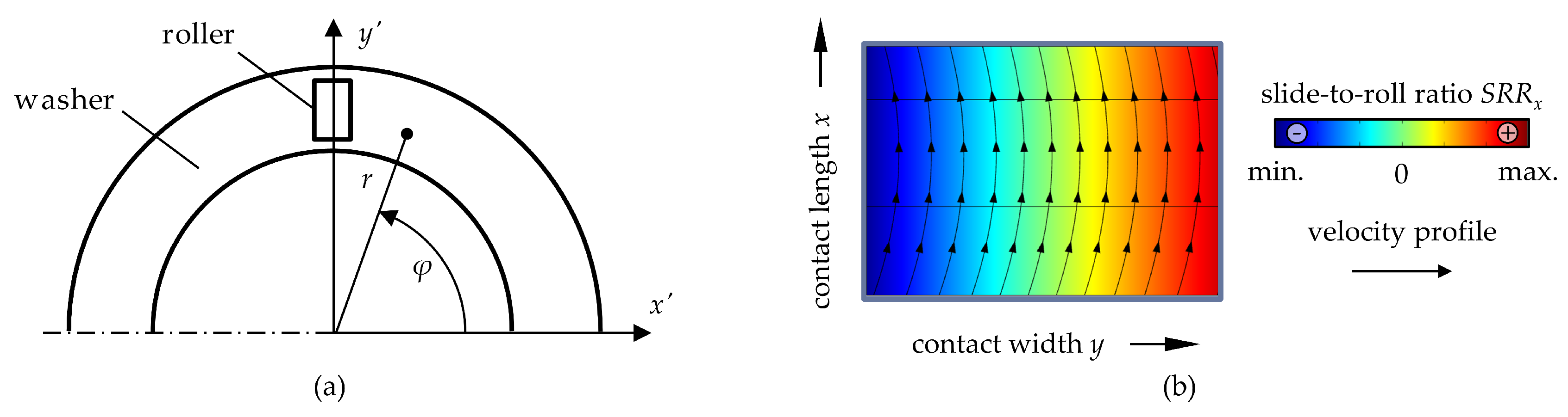
Underlying geometry and coordinates are illustrated in Figure 1.
It should be noted that the Cartesian coordinate system depicted in Figure 1 was rotated with the center of the considered rolling element. Thus, the resulting sliding velocity could be written as
A Young’s modulus of 210,000 MPa and a Poisson’s ratio of 0.3 were considered as the mechanical properties of the rollers and washers. Moreover, the surface height probability density function was assumed to be Gaussian with an equivalent standard deviation of σeq = 0.15 µm. Two mineral reference oil types with rather low viscosities were studied, for which the relevant lubricant properties are summed up in Table 2.
Density and viscosity were considered to be pressure-dependent following the equations from Dowson and Higginson [38] and Roelands [39], respectively:
Shear-thinning and thermal effects were neglected within the scope of this study and are subject of on-going research work.
2.2. Asperity Contact Model
An approach to calculate the real contact area and the load between an elastic rough surface and a rigid smooth plane based upon Hertzian-like deformations of asperities was first suggested by Greenwood and Williamson [40]. Since then, the model has been expanded, for example to take into account curved surfaces [41], two rough surfaces with misaligned asperities [42], elliptic paraboloid asperities [43] and anisotropic surfaces [44]. In addition, Chang et al. [25], Halling and Nuri [45], Zhao et al. [46] as well as Jamari and Schipper [47] developed analytical asperity contact models that allowed the consideration of elastic–plastic material properties. Moreover, Kogut and Etsion [29,30,31] as well as Jackson and Green [48,49] introduced FEM-based asperity contact models also taking into account elastic–plastic material behavior. Due to its broad applicability and simplicity, the Greenwood–Williamson model was used within the present study. It should be noted that all dimensionless values denoted by * were normalized by σ.
The asperity contact pressure in the dimensional form was given by
where is referred to as the reduced Young’s modulus:
Furthermore, denotes the probability density function of the asperity heights. Assuming a Gaussian distribution, the PDF normalized by the standard deviation of the surface heights σ resulted in:
Since the Greenwood–Williamson model used the mean of the summit heights as a reference and the mean of the surface heights was usually considered in EHL and by the applied Sugimura model, a transformation of the derived parameters was required. According to Nayak [50], Bush et al. [51] and McCool [44], the following relation between the standard deviation of asperity heights and surface heights applied:
whereas the bandwidth parameter α was defined by
The parameters m0 = σ2, m2 and m4 denote the zeroth, second and fourth spectral moments of a surface profile. Considering the density of summits:
and the mean summit radius:
led to the following relation between the standard deviation of the surface heights and the asperity heights:
The distance between the mean height of the asperities and the mean height of the surface according to Bush et al. [51] was:
Finally, the relation between the separation of a rough surface and a flat surface based on the asperity heights and surface heights reads:
The relation between the PDF of the summit heights and the PDF of the surface heights followed:
Taking into account two rough surfaces by the Greenwood–Williamson model is possible by calculating equivalent values for the standard deviation, the asperity radius and the asperity density according to Beheshti and Khonsari [52]:
2.3. EHL Modeling
In the context of higher loaded non-conformal contacts, CFD-based approaches, as suggested by Hartinger et al. [53,54], usually lead to high computational effort and instabilities at high loads. Consequently, numerical EHL modeling has frequently been done by applying the Reynolds equation [55] for hydrodynamics coupled with the solution of the elastic deformation. Therefore, iterative finite difference and half-space-based multilevel and multi-integration (MLMI) solvers, detailed in Venner and Lubrecht [56], are well established. Furthermore, Habchi et al. [57] introduced the full-system FEM-based approach to solve the system of fully coupled equations. This offered advantages in terms of computational effort and convergence behavior and most notably, enabled the use of commercially available software. Hence, the latter approach was used within the scope of this study.
Therefore, the Reynolds equation in a slightly modified form:
is solved in its weak form on the upper surface Ωc of the elastically deformed equivalent body (Figure 2) to describe the lubricant’s hydrodynamics. The first term describes the influence of the pressure gradient, while the second one accounts for the boundary velocities of the contacting bodies and the wedge-shape of the lubricant gap. Zero pressure boundary conditions were applied at the in- and outlet. A mass-conserving algorithm, as introduced by Marian et al. [58], dealt with cavitation effects. Therefore, the lubricant’s density and viscosity were multiplied with the fractional film content. The latter was defined as the ratio of the lubricant layer to the gap height:
with the penalty factor γ(ph), which is zero if ph < 0, otherwise γ(ph) = ξ, where ξ is a sufficiently high algebraic number. The Galerkin least squares (GLS) method (Hughes et al. [59]) and isotropic diffusion (Zienkiewicz et al. [60]) were utilized for the numerical stabilization.
Based upon the FEM, the elastic problem was calculated for one body Ω with the equivalent Young’s modulus:
and Poisson’s ratio:
by applying the linear elasticity equation:
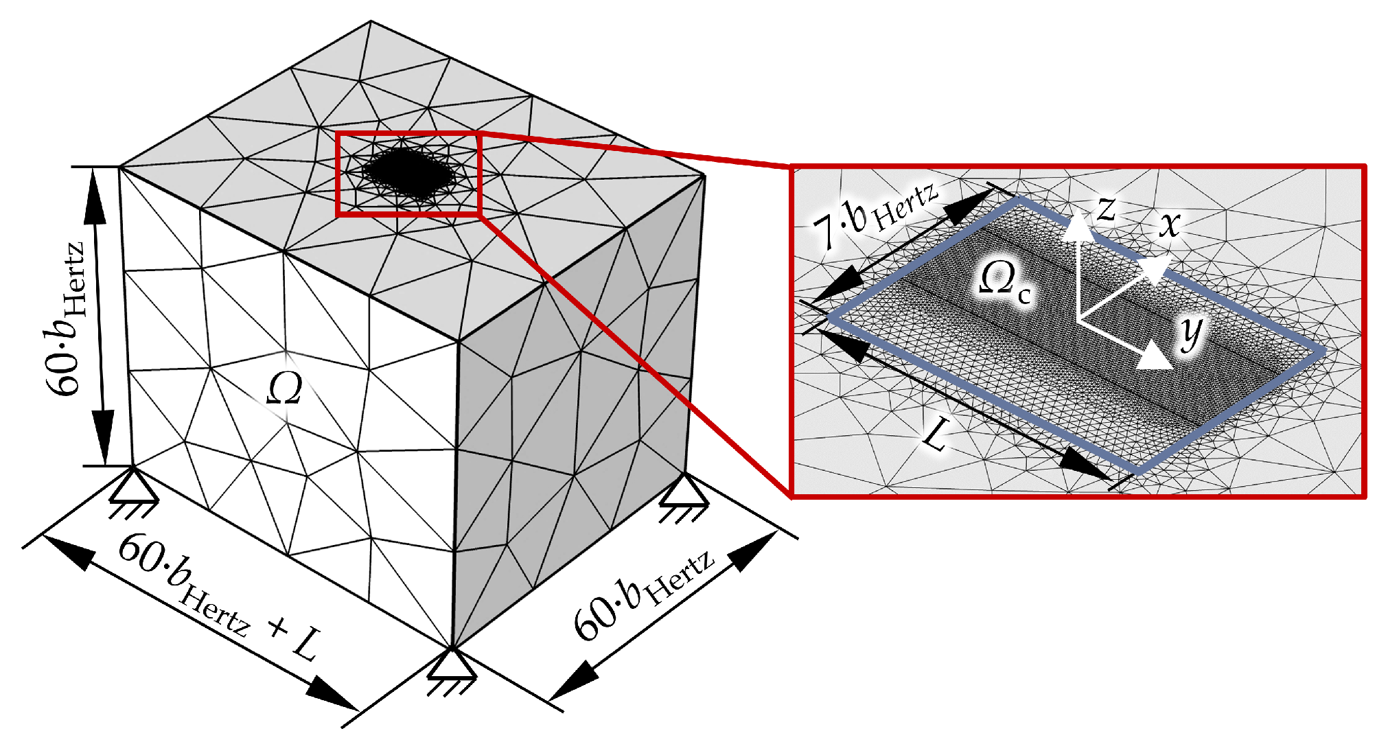
A free triangular mesh with a refinement in the contact center of the upper surface was applied and the body was provided with a zero-displacement boundary condition on the bottom and free boundary conditions on the sides. The dimensions of the cuboid were chosen large enough to exclude any effects on the calculation results [57]. Furthermore, a free triangular mesh with a refinement in the contact center of the upper surface was applied. Geometry and meshing are schematically illustrated in Figure 2.
The lubricant film thickness equation:
describes the height of the separating fluid film in terms of the distance and the shape of the undeformed geometry as well as of the elastic deformation. The geometry of the rolling element was composed of a quadratic approximation of the radius in and the logarithmic profile perpendicular to the direction of motion:
The load balance equation:
ensures the equilibrium of forces, taking into account simultaneously occurring asperity contact (Section 2.1.) and hydrodynamic lubrication by a stochastic mixed lubrication [61].
In order to obtain a consistent model without regenerating and remeshing the computational domains at different load cases as well as to avoid instabilities due to memory variables with limited accuracy, all the solution variables were normalized to characteristic quantities of the Hertzian theory or, in the case of the lubricant, initial values:
In addition, the computational domain was decreased in y direction by the factor scale in order to reduce the number of degrees of freedom and thus the computation time.
2.4. Wear Modeling
Widely used wear models were proposed by Kragelski [62] and Fleischer et al. [63]. The first developed a molecular mechanical fatigue-based wear model and the approach of the latter considered the frictional energy density. However, the most common model for calculating wear, originally intended for dry contacts, goes back to Archard [5,64] and Holm [65]. Although various other wear modeling approaches, based upon empirical relationships or limited to specific applications, exist in the literature, Archard’s wear model was applied within the scope of this contribution for its generality and simplicity. Thereby, the total wear volume Vw was considered proportional to the normal force FN, the sliding distance s and the proportionality factor k, also known as the wear coefficient:
To calculate the wear in a lubricated contact, the Archard wear model, which in its conventional form is valid for dry contacts, was modified assuming that wear could only occur on a solid asperity contact:
As a result, the local wear depth was derived by
Since the wear coefficient depends on numerous factors, such as material properties, surface conditions and boundary layers, it was frequently determined experimentally and could vary between 10−1 and 10−15 mm3/Nm for metals [66,67]. As it can be assumed that even under the highest loads, some protecting boundary layer will be formed and that at least some lubricant will remain in the contact between the two opposing asperities, it seems appropriate in the context of the present study to apply a wear coefficient that is valid for the boundary lubrication regime in order to calculate the wear depth. In accordance to Czichos and Habig [68], a local wear coefficient of was applied.
2.5. Surface Topography Model
The Sugimura model [32,33,34] was used to take into account the wear-induced change of statistical surface parameters within the asperity contact pressure calculation.
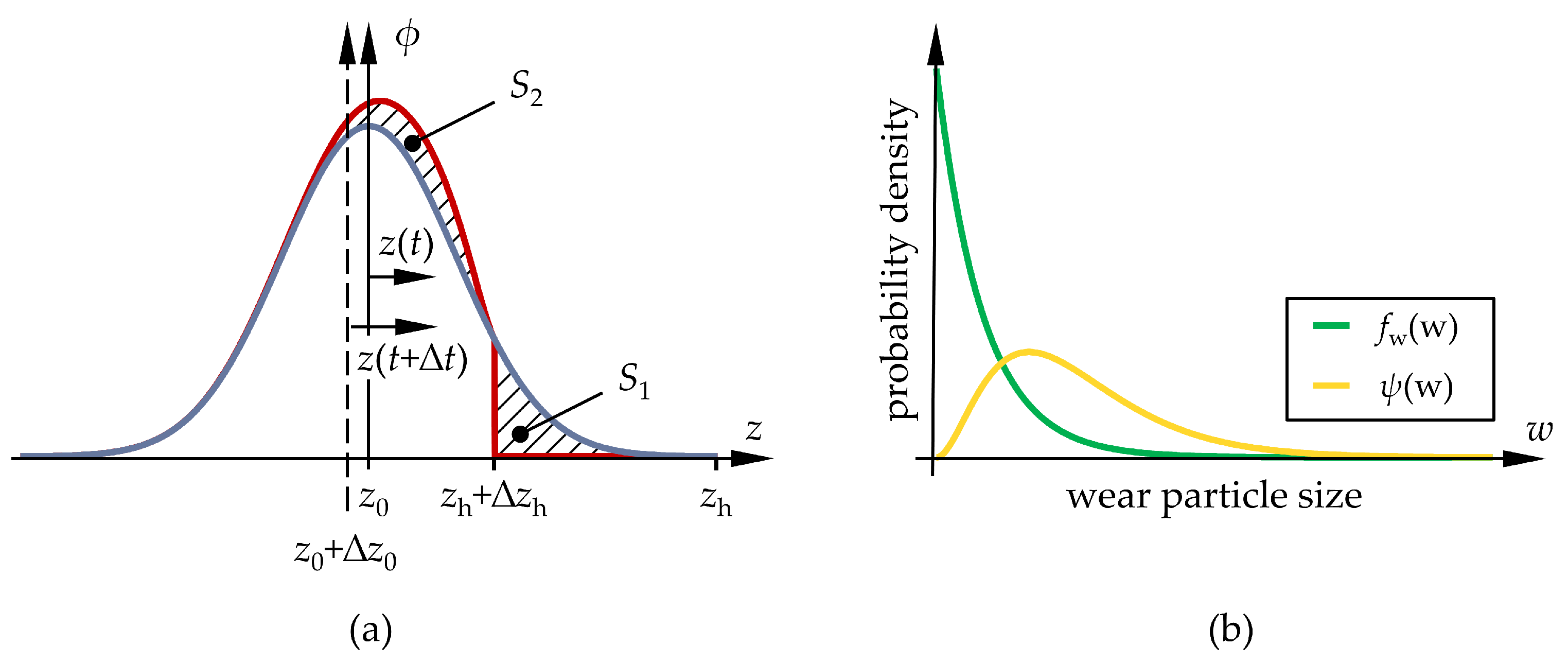
Assuming an arbitrary distribution of the initial surface heights, the upper proportion of the probability distribution S1 was removed, as schematically illustrated in Figure 3a, depending on the wear depth W and the mean wear-related height loss :
where:
Thereby, ψ denotes the probability density function of the wear-induced height loss and could be derived from the wear particle size distribution:
where u, v, and w are the wear particle dimensions. Additionally, f(u,v,w) denotes the probability density function of the wear particle size. Assuming the proportionality of u and v to w results in:
with the marginal density function of the wear particle density function:
Following Kimura and Sugimura [34], an exponential distribution for the wear particle size, as depicted in Figure 3b, was assumed. Finally, the fraction of the removed surface PDF was then redistributed to the remaining density function accordingly (Figure 3a). The surface height probability density function at the time t + Δt was written by considering the shift of the mean height Δz0:
where the shift of the mean height satisfies:
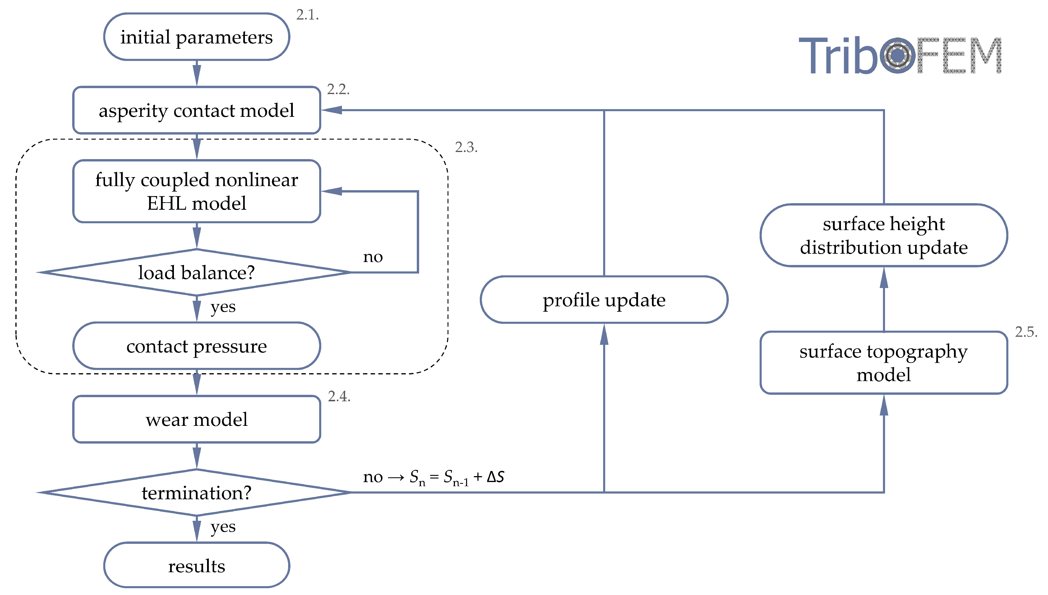
2.6. Overall Numerical Procedure
The global numerical solution scheme is presented in Figure 4. Based upon the initial parameters on bulk material, surface topography and lubricant rheology (see Section 2.1), the asperity contact pressure in dependency of the mean surface distance was calculated according to the Greenwood–Williamson model as described in Section 2.2 using MATHWORKS MATLAB. Subsequently, the system of highly nonlinear EHL equations, see Section 2.3, was solved fully coupled utilizing COMSOL MULTIPHYSICS. For more fundamental aspects about FEM in EHL and further information about the implementation, the interested reader is referred to Habchi [69]. After convergence, the wear evolution was calculated based upon the resulting solid contact pressure using Archard’s law as described in Section 2.4 and the profile was updated accordingly. Moreover, the PDF of the surface heights was adapted using the Sugimura model, see Section 2.5. These steps were also implemented in MATHWORKS MATLAB and repeated until the intended operating period of the thrust roller bearing was reached.
It should be noted that each of the individual aforementioned sub-models (Section 2.2, Section 2.3, Section 2.4 and Section 2.5) used within the scope of this contribution were chosen based upon their similar degree of complexity and good implementability. However, they could in principle be replaced by any other or more sophisticated models.
3. Results and Discussion
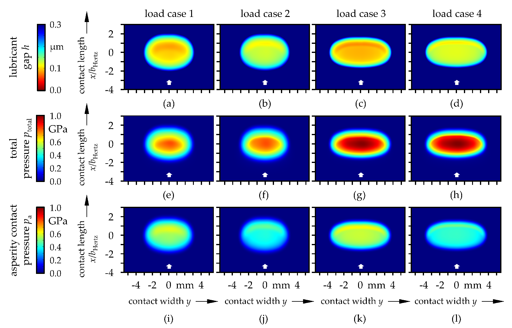
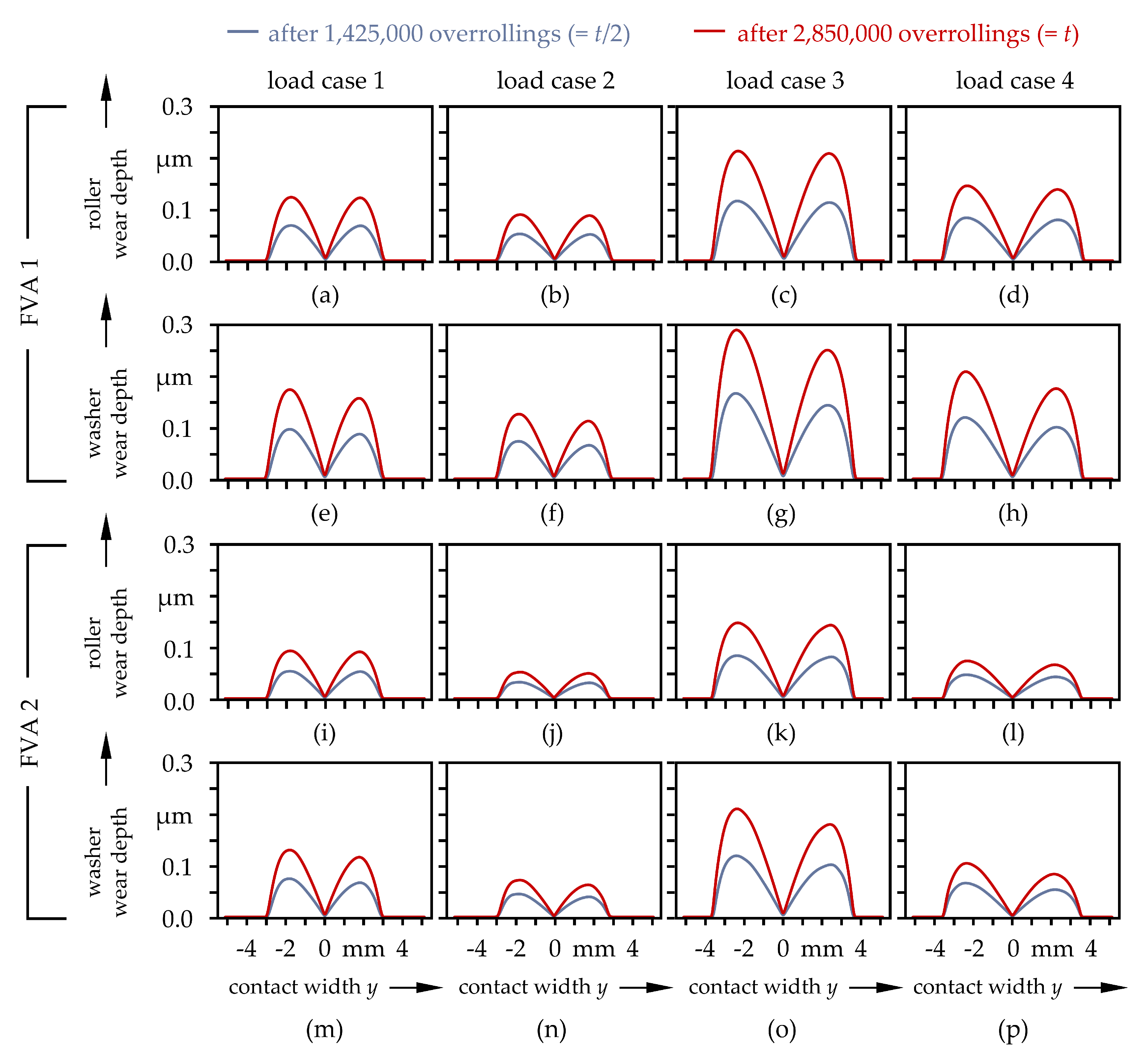
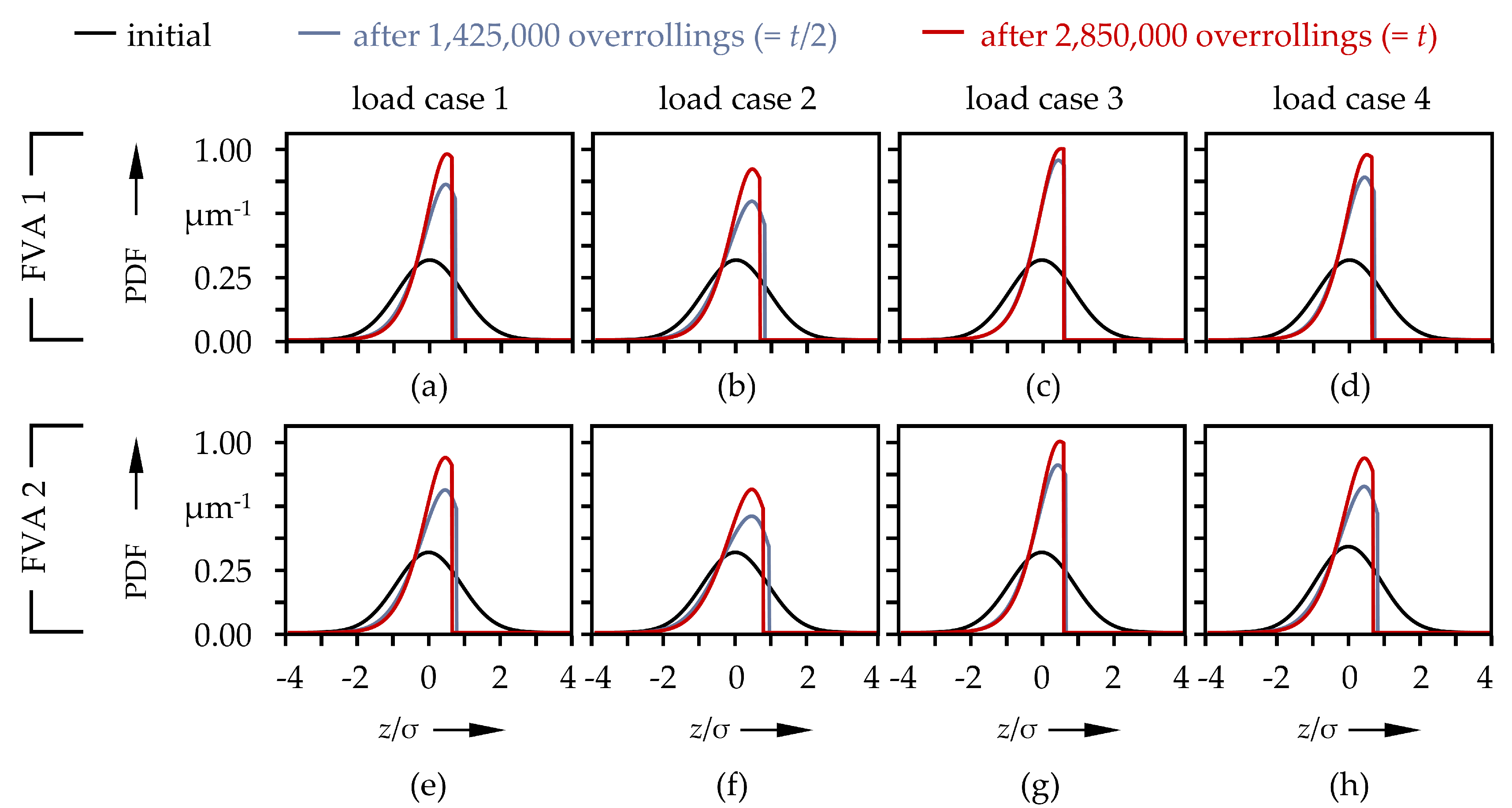
The lubrication conditions of all four load cases and both oil types in terms of fluid film gap and total and solid contact pressure are depicted in Figure 5 and Figure 6 and Figures 10–13. The value ranges of the result variables are set equal in all figures to ensure easy comparability. The scales were chosen in such a way that the relevant effects are properly visualized and actual extrema are partially not mapped. Furthermore, the wear profiles of the rolling elements and washers as well as the probability density function and the asperity contact pressure function are shown in Figure 7, Figure 8 and Figure 9 for several time-steps. The calculated mass losses are then summarized in Table 3.
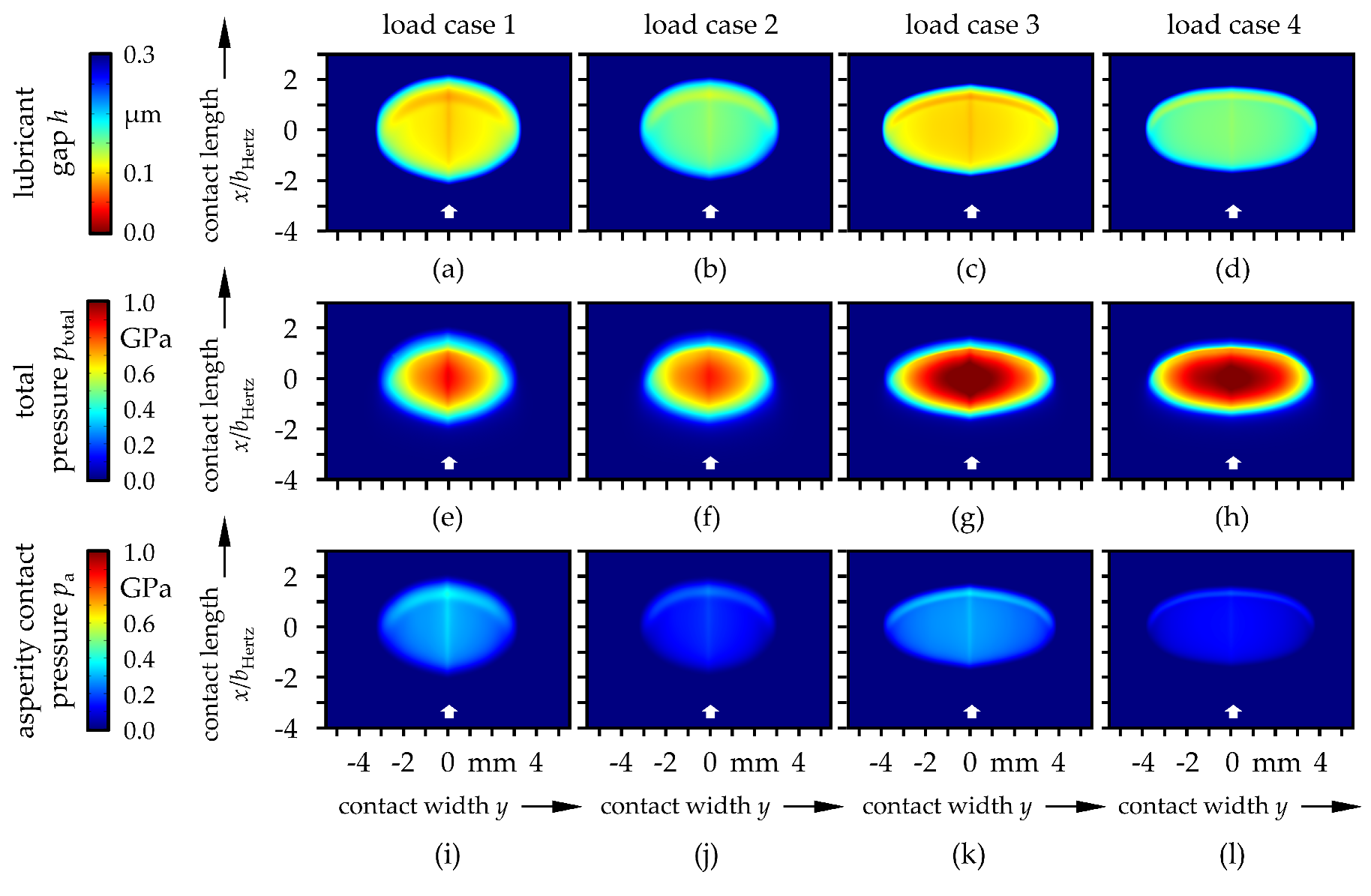
Due to the roller radius in and the logarithmic profile perpendicular to the direction of motion, the initial conditions featured typical characteristics for elliptical EHL contacts with a horseshoe-shaped lubricant gap (Figure 5a–d), a total pressure distribution similar to Hertz (Figure 5e–h) as well as a constriction in the film height as well as a barely pronounced Petrusevich spike in the outlet region. Due to the smaller contact area, the pressures exceeded the Hertzian values determined for a perfect line contact (Table 1). In addition, the speed profile (Figure 1b) resulted in a slight asymmetry and tilting of the contact area. The clearly recognizable asperity contact pressure (Figure 5i–l) followed the lubricant height in shape and indicated an operation under mixed EHL conditions. The effects of the load case and oil on the lubricant gap and the pressure formation basically corresponded to theoretical expectations. Higher speed (load case 2) and higher viscosity (Figure 6) led to a larger and higher load (load case 3, 4) to a lower fluid film height. Accordingly, the asperity contact pressure behaved just oppositely. Moreover, the higher load led to a significantly larger elastically deformed contact area. It should be noted that although the contact width y was scaled in the same way for all cases, the contact length x was plotted normalized to the Hertzian width for reasons of reduced space requirements. Thus, the contact area actually expanded further in the x direction at higher loads as well.
The continuous progress of the simulated time led to material loss and changes of the surface topography of the washers and the rollers. In brief, the wear-depth distribution, as depicted in Figure 7, followed the product of asperity contact pressure and sliding velocity. The inner (negative y values) and outer halves (positive y values) of the raceway showed a slightly asymmetrical shape due to different velocities. Thereby, wear was higher in the area of the negative slip. This stands in good agreement with the experimental results from Terwey et al. [13,14]. Despite differences in absolute values due to the less severe conditions (lower loads and higher velocities) and the operation being in the mixed instead of the boundary lubrication regime, the qualitative profiles agree well. Furthermore, a more significant difference in the wear depth between the inner and outer halves of the raceway could be found on the washer. This was due to the fact that the calculated wear volume was distributed over a smaller circumference at the inner half of the raceway than at the outer area. Higher loads and lower sliding velocities resulted in a higher wear depth. This can be explained by lower lubricating film heights resulting in higher asperity contact pressures. For the same reason, the use of a lower viscosity oil (FVA1) compared to a higher viscosity oil (FVA 2) led to higher wear depths.
Proceeding wear also resulted in an adjustment of the probability density function of asperity heights, see Figure 8. By applying Sugimura’s wear model, the probability density function of the surface heights was recalculated and adapted in each time step of the wear simulation assuming an exponentially distributed wear particle size. With a further continuing wear process, the PDF reached a stationary shape. This can be seen the most for the wear-intensive load case 3 with lower-viscosity oil FVA 1 (see Figure 8c). Here, the PDF of the surface heights after half of the simulation time only differed slightly from the PDF at the end of the wear simulation, indicating a run-in surface topography.
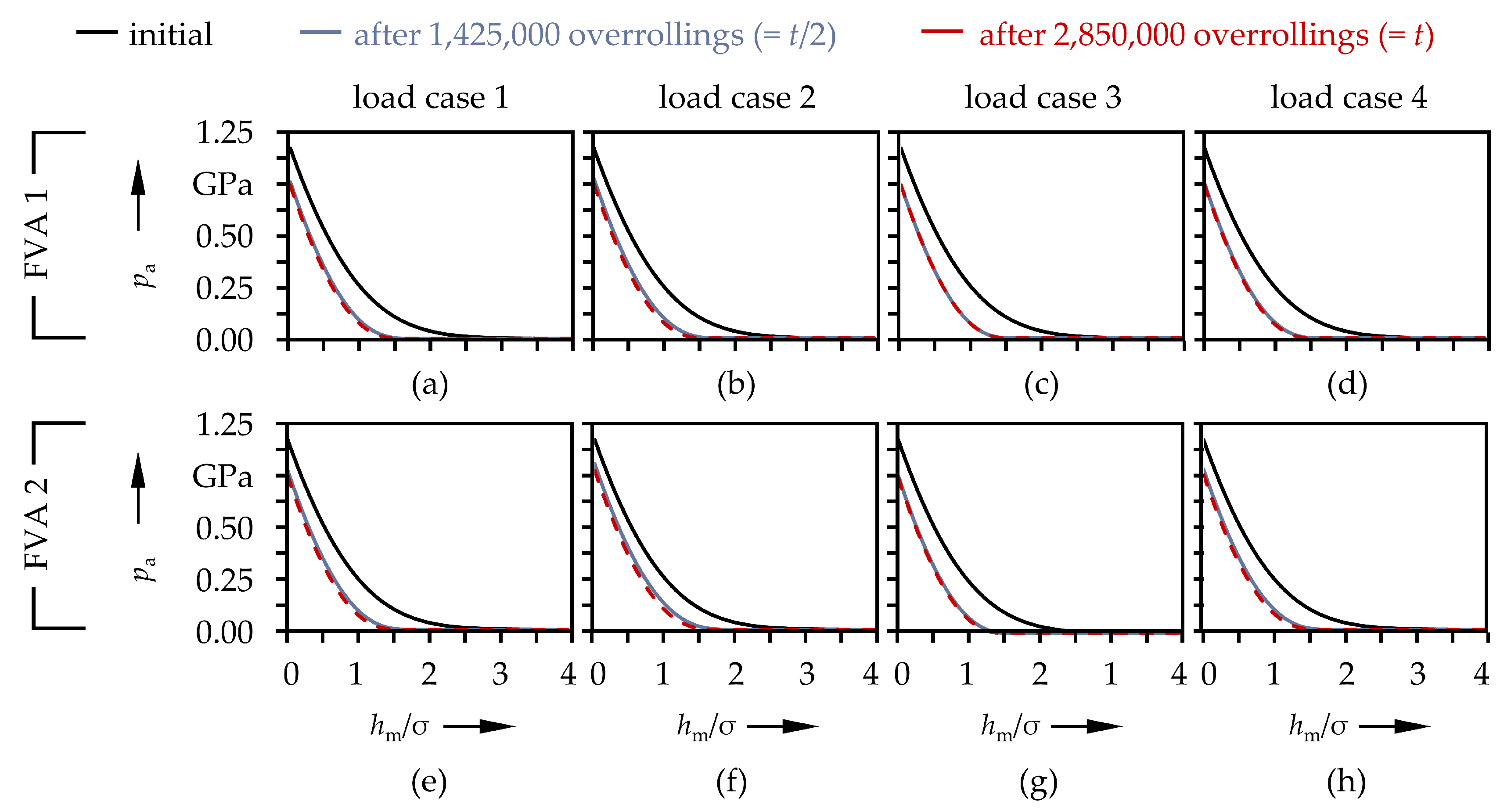
The PDF of the asperity heights were further applied to the calculation of the asperity contact pressures, which were a prerequisite for the application of the mixed friction model based upon the load sharing concept. As can be seen in Figure 9, the contact pressures were shifted to the bottom left with increasing simulation time, which was caused by the worn-out asperity peaks in terms of the modified probability density functions. Furthermore, in most cases the asperity contact pressure curves also reached a stationary state with slight differences to the final state being distinguishable for less harmful cases, see for example Figure 9f).
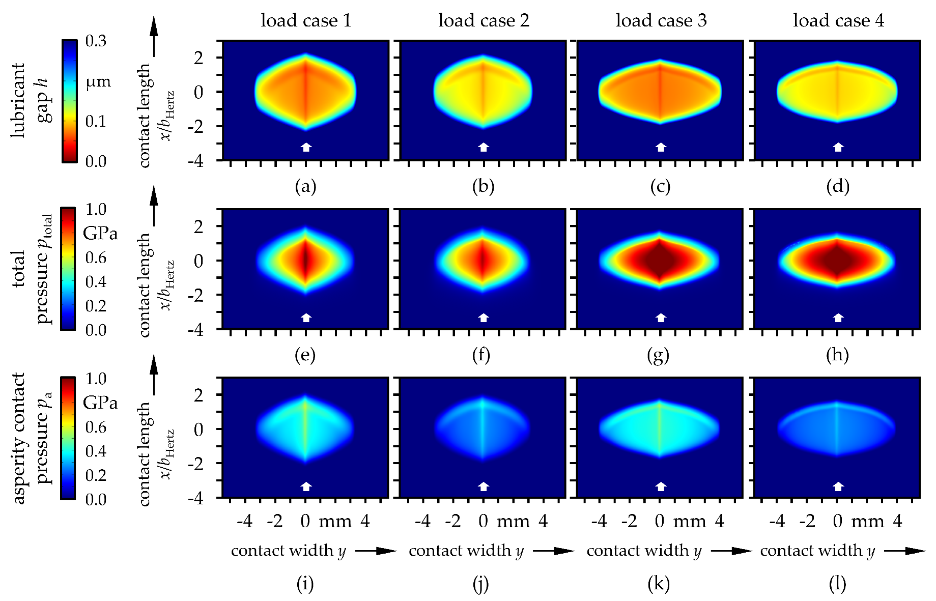
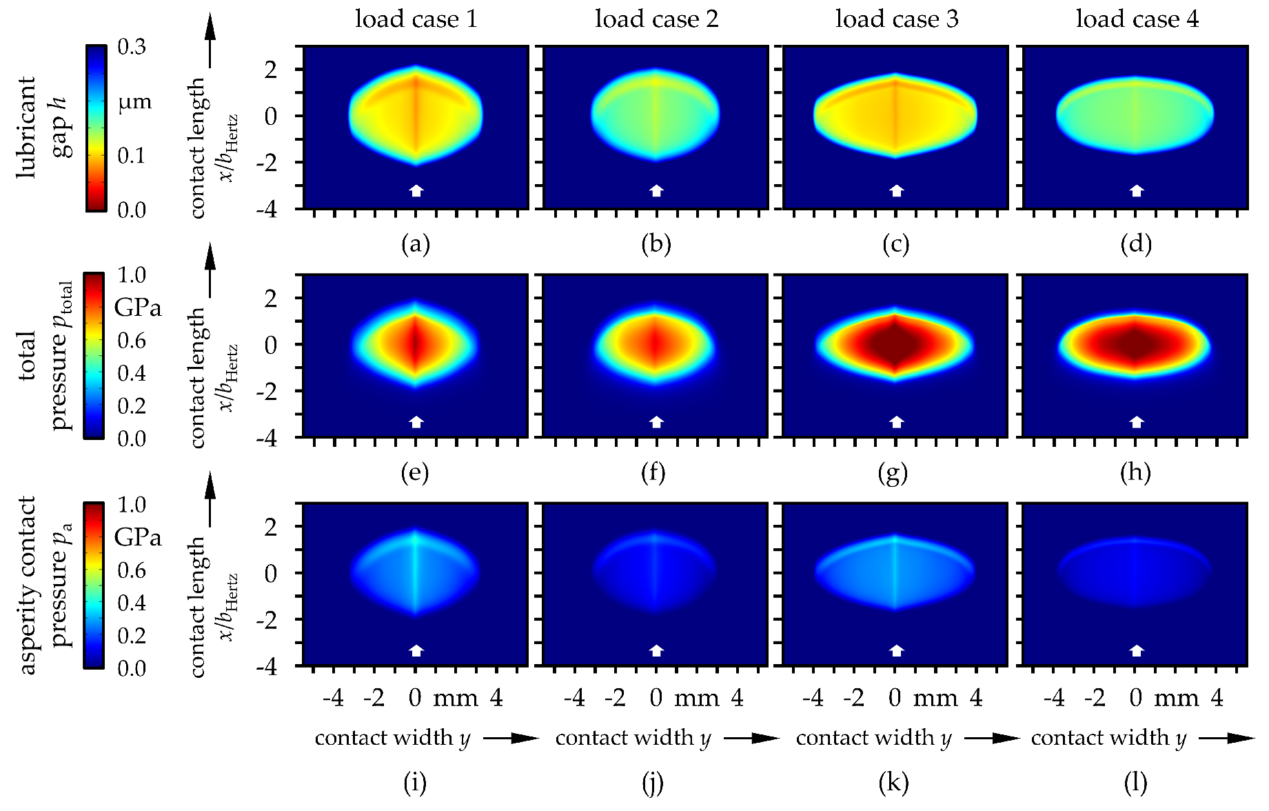
Changes in the surface topography were also accompanied by transformations of the lubrication conditions, see Figure 10, Figure 11, Figure 12 and Figure 13. In addition to the horseshoe-shaped constriction of the lubricant gap at the contact outlet region, there was a similarly pronounced minimum along the y = 0 axis. This was due to the low wear in this area, despite the high total and asperity contact pressure, since the conditions of the pure rolling (slide-to-roll ratio (SRR) = 0) prevailed. Furthermore, the asymmetry and slight tilting resulting from the speed and wear profiles could still be observed. Generally, the distributions of the lubricant gap and the pressure continued to correspond to the principles of the influences of speed, load and viscosity. In most cases, the fluid and pressure distribution only featured small differences between the half and end of the simulation time. While some load cases still showed significant asperity contact pressure after the simulated runtime, see Figure 12i,k), others indicated a kind of completed running-in process with hardly any solid contact compared to the initial state, see for example Figure 13l).
Finally, the calculated wear masses for both bearing washers and all the rolling elements of the studied 81212 thrust roller bearing are summarized in Table 3. Again, it can be seen that the highest wear mass was calculated for load case 3 (highest load, lowest speed) in combination with the lower viscosity oil FVA 1. In contrast, load case 2 (lowest load, highest speed) in combination with the higher viscosity oil FVA 2 resulted in the lowest total wear.
4. Conclusions
Within the scope of this contribution, a numerical simulation method for studying the wear evolution of a thrust roller bearing under mixed elastohydrodynamic lubrication was introduced. Therefore, realistic geometries and operating conditions, especially a local velocity distribution, were considered. During the simulation time, the macroscopic lubrication conditions obtained by a FEM-based 3D EHL model were coupled with macroscopic and microscopic surface topography changes following a local Archard-type wear model, a Greenwood–Williamson-based load-sharing approach and the Sugimura surface adaption model. The simulations, carried out by means of four load cases and two different mineral oil types, indicated clear differences in the wear behavior, whereby stronger wear was favored by a lower velocity, higher load and lower oil viscosity. Thereby, asymmetrical wear profiles on the rollers and washers were revealed, whereas a negative slip on the outer half resulted in more a pronounced wear compared to the positive slip on the inner half of the raceway. This could be attributed to the velocity and slip distribution. Thus, the obtained results corresponded qualitatively well with the experimental results from the literature. In the future, it is intended to further enhance the EHL model by taking into account thermal and non-Newtonian effects. The use of locally modified probability density and asperity contact functions will also improve the prediction quality. However, the presented numerical simulation procedure already enables the determination of harmful load case and fluid property combinations. Moreover, the approach could be used to derive suitable running-in procedures.
Author Contributions
Conceptualization, A.W. and M.M.; methodology, A.W. and M.M.; software, A.W.; formal analysis, A.W. and M.M.; writing—original draft preparation, A.W. and M.M.; writing—review and editing, A.W., M.M., S.T. and S.W.; visualization, A.W. and M.M.; supervision, S.T. and S.W. All authors have read and agreed to the published version of the manuscript.
Funding
This research received no external funding.
Acknowledgments
The authors greatly acknowledge the continuous support of the Friedrich-Alexander-Universität Erlangen-Nürnberg (FAU), Germany.
Conflicts of Interest
The authors declare no conflict of interest.
Nomenclature
| bHertz | Hertzian contact half-width |
| C | compliance matrix |
| d | separation based on asperity heights |
| D | diameter of roller |
| E’ | reduced Young’s modulus |
| E1, E2 | Young’ modulus of washer/roller |
| Eeq | equivalent Young’s modulus |
| f | probability density function of the wear particle size |
| fw | marginal density function of the wear particle density function |
| F | bearing load |
| FN | normal contact force |
| h | lubricant gap |
| h0 | film thickness constant parameter |
| hliq | lubricant film thickness |
| hw | local wear depth |
| H | dimensionless lubricant gap |
| k | global wear coefficient |
| local wear coefficient | |
| L | length of roller |
| m0,2,4 | zeroth, second and fourth spectral moment of a surface profile |
| n | rotational speed |
| pa | asperity contact pressure |
| ph | fluid pressure |
| pHertz | Hertzian contact pressure |
| ptotal | total pressure |
| P | dimensionless pressure |
| Rx | radius of curvature in x direction |
| s | sliding distance |
| s0 | geometry-function of the roller |
| SRR | slide-to-roll ratio |
| t | test duration |
| u, v, w | size of cuboid shaped wear particle |
| u1,u2 | relative velocity of the washer/roller in x direction |
| U | displacement tensor |
| Uz | displacement in z direction |
| v1,v2 | relative velocity of the washer/roller in y direction |
| vslip | slip velocity |
| Vw | wear volume |
| mean height loss | |
| W | mean wear depth |
| x,y | coordinates in and perpendicular to the rolling direction |
| X, Y | dimensionless coordinates in and perpendicular to the rolling direction |
| ys | distance between the mean height of asperities and the mean height of surface |
| z | profile coordinate based on mean height of surface |
| zs | profile coordinate based on mean height of asperities |
| z0 | ordinate of the mean line of the composite profile |
| Δz0 | descending quantity of mean line |
| zh | highest point of composite profile |
| Δzh | moving distance of highest point |
| α | bandwidth parameter |
| αp | pressure-viscosity coefficient |
| β | mean summit radius |
| γ | penalty function |
| elastic deformation in z direction | |
| dimensionless elastic deformation in z direction | |
| ε | strain tensor |
| ν1, ν2 | Poisson’s ratio of washer/roller |
| νeq | equivalent Poisson’s ratio |
| lubricant density | |
| dimensionless lubricant density | |
| lubricant density at reference state (40 °C) | |
| η | lubricant viscosity |
| dimensionless lubricant viscosity | |
| η0 | lubricant viscosity at reference state (40 °C) |
| ηs | area density of asperities |
| θ | fractional film content |
| σ | standard deviation of surface heights |
| σelastic | stress tensor of the equivalent body |
| σs | standard deviation of asperity heights |
| ϕ | probability density function of surface heights |
| ϕs | probability density function of asperity heights |
| ψ | height-loss probability density function |
| ω | angular velocity |
| Ωc | contact domain |
References
- Holmberg, K.; Erdemir, A. Influence of tribology on global energy consumption, costs and emissions. Friction 2017, 5, 263–284. [Google Scholar] [CrossRef]
- Holmberg, K.; Andersson, P.; Erdemir, A. Global energy consumption due to friction in passenger cars. Tribol. Int. 2012, 47, 221–234. [Google Scholar] [CrossRef]
- Põdra, P.; Andersson, S. Simulating sliding wear with finite element method. Tribol. Int. 1999, 32, 71–81. [Google Scholar] [CrossRef]
- Põdra, P.; Andersson, S. Wear simulation with the Winkler surface model. Wear 1997, 207, 79–85. [Google Scholar] [CrossRef]
- Archard, J.F. Contact and Rubbing of Flat Surfaces. Proc. R. Soc. A Math. Phys. Eng. Sci. 1953, 24, 981–988. [Google Scholar] [CrossRef]
- Winkler, E. Die Lehre von der Elasticitaet und Festigkeit: Mit Besonderer Rücksicht auf Ihre Anwendung in der Technik für Polytechnische Schulen, Bauakademien, Ingenieue, Maschinenbauer, Architecten, etc; Dominicus: Prague, Austria-Hungary, 1868. [Google Scholar]
- Hegadekatte, V.; Huber, N.; Kraft, O. Modeling and simulation of wear in a pin on disc tribometer. Tribol. Lett. 2006, 24, 51–60. [Google Scholar] [CrossRef]
- Hegadekatte, V.; Kurzenhäuser, S.; Huber, N.; Kraft, O. A predictive modeling scheme for wear in tribometers. Tribol. Int. 2008, 41, 1020–1031. [Google Scholar] [CrossRef] [Green Version]
- Andersson, J.; Almqvist, A.; Larsson, R. Numerical simulation of a wear experiment. Wear 2011, 271, 2947–2952. [Google Scholar] [CrossRef]
- Liu, S.; Wang, Q.; Liu, G. A versatile method of discrete convolution and FFT (DC-FFT) for contact analyses. Wear 2000, 243, 101–111. [Google Scholar] [CrossRef]
- Ashraf, M.A.; Ahmed, R.; Ali, O.; Faisal, N.H.; El-Sherik, A.M.; Goosen, M.F.A. Finite Element Modeling of Sliding Wear in a Composite Alloy Using a Free-Mesh. J. Tribol. Trans. ASME 2015, 137, 27. [Google Scholar] [CrossRef]
- Sfantos, G.; Aliabadi, M. A boundary element formulation for three-dimensional sliding wear simulation. Wear 2007, 262, 672–683. [Google Scholar] [CrossRef]
- Terwey, J.T.; Berninger, S.; Burghardt, G.; Jacobs, G.; Poll, G. Numerical Calculation of Local Adhesive Wear in Machine Elements Under Boundary Lubrication Considering the Surface Roughness. In Proceedings of the 7th International Conference on Fracture Fatigue and Wear; Abdel Wahab, M., Ed.; Springer: Singapore, 2019; pp. 796–807. ISBN 978-981-13-0410-1. [Google Scholar]
- Terwey, J.T.; Fourati, M.A.; Pape, F.; Poll, G. Energy-Based Modelling of Adhesive Wear in the Mixed Lubrication Regime. Lubricants 2020, 8, 16. [Google Scholar] [CrossRef] [Green Version]
- Zhu, N.; Martini, A.; Wang, W.; Hu, Y.; Lisowsky, B.; Wang, Q.J. Simulation of Sliding Wear in Mixed Lubrication. J. Tribol. 2007, 129, 544–552. [Google Scholar] [CrossRef]
- Zhu, N.; Hu, Y.-Z. A Computer Program Package for the Prediction of EHL and Mixed Lubrication Characteristics, Friction, Subsurface Stresses and Flash Temperatures Based on Measured 3-D Surface Roughness. Tribol. Trans. 2001, 44, 383–390. [Google Scholar] [CrossRef]
- Hu, Y.-Z.; Zhu, N. A Full Numerical Solution to the Mixed Lubrication in Point Contacts. J. Tribol. 1999, 122, 1–9. [Google Scholar] [CrossRef]
- Lorentz, B.; Albers, A. A numerical model for mixed lubrication taking into account surface topography, tangential adhesion effects and plastic deformations. Tribol. Int. 2013, 59, 259–266. [Google Scholar] [CrossRef]
- Reichert, S.; Lorentz, B.; Heldmaier, S.; Albers, A. Wear simulation in non-lubricated and mixed lubricated contacts taking into account the microscale roughness. Tribol. Int. 2016, 100, 272–279. [Google Scholar] [CrossRef]
- Johnson, G.R.; Cook, W.H. Fracture characteristics of three metals subjected to various strains, strain rates, temperatures and pressures. Eng. Fract. Mech. 1985, 21, 31–48. [Google Scholar] [CrossRef]
- Beheshti, A.; Khonsari, M.M. A Thermodynamic Approach for Prediction of Wear Coefficient Under Unlubricated Sliding Condition. Tribol. Lett. 2010, 38, 347–354. [Google Scholar] [CrossRef]
- Akbarzadeh, S.; Khonsari, M.M. Thermoelastohydrodynamic Analysis of Spur Gears with Consideration of Surface Roughness. Tribol. Lett. 2008, 32, 129–141. [Google Scholar] [CrossRef]
- Beheshti, A.; Khonsari, M.M. An engineering approach for the prediction of wear in mixed lubricated contacts. Wear 2013, 308, 121–131. [Google Scholar] [CrossRef]
- Hao, L.; Meng, Y. Numerical Prediction of Wear Process of an Initial Line Contact in Mixed Lubrication Conditions. Tribol. Lett. 2015, 60, 443. [Google Scholar] [CrossRef]
- Chang, W.-R.; Etsion, I.; Bogy, D.B. An Elastic-Plastic Model for the Contact of Rough Surfaces. J. Tribol. 1987, 109, 257–263. [Google Scholar] [CrossRef]
- Zhang, Y.; Kovalev, A.; Hayashi, N.; Nishiura, K.; Meng, Y. Numerical Prediction of Surface Wear and Roughness Parameters During Running-In for Line Contacts Under Mixed Lubrication. J. Tribol. Trans. ASME 2018, 140, 061501. [Google Scholar] [CrossRef]
- Patir, N.; Cheng, H.S. An Average Flow Model for Determining Effects of Three-Dimensional Roughness on Partial Hydrodynamic Lubrication. J. Lubr. Technol. 1978, 100, 12–17. [Google Scholar] [CrossRef]
- Patir, N.; Cheng, H.S. Application of Average Flow Model to Lubrication Between Rough Sliding Surfaces. J. Lubr. Technol. 1979, 101, 220–229. [Google Scholar] [CrossRef]
- Kogut, L.; Etsion, I. Elastic-Plastic Contact Analysis of a Sphere and a Rigid Flat. J. Appl. Mech. 2002, 69, 657–662. [Google Scholar] [CrossRef] [Green Version]
- Kogut, L.; Etsion, I. A Finite Element Based Elastic-Plastic Model for the Contact of Rough Surfaces. Tribol. Trans. 2003, 46, 383–390. [Google Scholar] [CrossRef]
- Kogut, L.; Etsion, I. A Static Friction Model for Elastic-Plastic Contacting Rough Surfaces. J. Tribol. 2004, 126, 34–40. [Google Scholar] [CrossRef]
- Sugimura, J.; Kimura, Y. Characterization of topographical changes during lubricated wear. Wear 1984, 98, 101–116. [Google Scholar] [CrossRef]
- Sugimura, J.; Kimura, Y.; Amino, K. Analysis of the topographical changes due to wear—Geometry of the running-in process. J. Jpn. Soc. Lubr. Eng. 1986, 31, 813–820. [Google Scholar]
- Kimura, Y.; Sugimura, J. Microgeometry of sliding surfaces and wear particles in lubricated contact. Wear 1984, 100, 33–45. [Google Scholar] [CrossRef]
- Zhang, Y.; Cao, H.; Kovalev, A.; Meng, Y. Numerical Running-In Method for Modifying Cylindrical Roller Profile Under Mixed Lubrication of Finite Line Contacts. J. Tribol. 2019, 141, 041401. [Google Scholar] [CrossRef]
- Evans, H.; Snidle, B. Analysis of micro-elastohydrodynamic lubrication for engineering contacts. Tribol. Int. 1996, 29, 659–667. [Google Scholar] [CrossRef]
- Johnson, K.; Greenwood, J.A.; Poon, S. A simple theory of asperity contact in elastohydro-dynamic lubrication. Wear 1972, 19, 91–108. [Google Scholar] [CrossRef]
- Dowson, D.; Higginson, G.R. Elasto-Hydrodynamic Lubrication: The Fundamentals of Roller and Gear Lubrication; Pergamon Press: Oxford, UK, 1966. [Google Scholar]
- Roelands, C.J.A.; Winer, W.O.; Wright, W.A. Correlational Aspects of the Viscosity-Temperature-Pressure Relationship of Lubricating Oils (Dr In dissertation at Technical University of Delft, 1966). J. Lubr. Technol. 1971, 93, 209–210. [Google Scholar] [CrossRef] [Green Version]
- Greenwood, J.A.; Williamson, J.B.P. Contact of nominally flat surfaces. Proc. R. Soc. A Math. Phys. Eng. Sci. 1966, 295, 300–319. [Google Scholar] [CrossRef]
- Greenwood, J.A.; Tripp, J.H. The Elastic Contact of Rough Spheres. J. Appl. Mech. 1967, 34, 153–159. [Google Scholar] [CrossRef]
- Greenwood, J.A.; Tripp, J.H. The Contact of Two Nominally Flat Rough Surfaces. Proc. Inst. Mech. Eng. 1970, 185, 625–633. [Google Scholar] [CrossRef]
- Bush, A.; Gibson, R.; Thomas, T. The elastic contact of a rough surface. Wear 1975, 35, 87–111. [Google Scholar] [CrossRef]
- McCool, J.I. Comparison of models for the contact of rough surfaces. Wear 1986, 107, 37–60. [Google Scholar] [CrossRef]
- Halling, J.; Nuri, K. Elastic/plastic contact of surfaces considering ellipsoidal asperities of work-hardening multi-phase materials. Tribol. Int. 1991, 24, 311–319. [Google Scholar] [CrossRef]
- Zhao, Y.; Maietta, D.M.; Chang, L. An Asperity Microcontact Model Incorporating the Transition From Elastic Deformation to Fully Plastic Flow. J. Tribol. 2000, 122, 86. [Google Scholar] [CrossRef]
- Jamari, J.; Schipper, D.J. An elastic–plastic contact model of ellipsoid bodies. Tribol. Lett. 2006, 21, 262–271. [Google Scholar] [CrossRef]
- Jackson, R.L.; Green, I. A Finite Element Study of Elasto-Plastic Hemispherical Contact Against a Rigid Flat. J. Tribol. 2005, 127, 343–354. [Google Scholar] [CrossRef] [Green Version]
- Jackson, R.L.; Green, I. A statistical model of elasto-plastic asperity contact between rough surfaces. Tribol. Int. 2006, 39, 906–914. [Google Scholar] [CrossRef]
- Nayak, P.R. Random Process Model of Rough Surfaces. J. Lubr. Technol. 1971, 93, 398–407. [Google Scholar] [CrossRef]
- Bush, A.; Gibson, R.; Keogh, G. The limit of elastic deformation in the contact of rough surfaces. Mech. Res. Commun. 1976, 3, 169–174. [Google Scholar] [CrossRef]
- Beheshti, A.; Khonsari, M.M. Asperity micro-contact models as applied to the deformation of rough line contact. Tribol. Int. 2012, 52, 61–74. [Google Scholar] [CrossRef]
- Hartinger, M.; Dumont, M.-L.; Ioannides, S.; Gosman, D.; Spikes, H. CFD Modeling of a Thermal and Shear-Thinning Elastohydrodynamic Line Contact. J. Tribol. 2008, 130, 041503. [Google Scholar] [CrossRef]
- Hartinger, M.; Gosman, D.; Ioannides, S.; Spikes, H. Two-and Three-Dimensional CFD Modelling of Elastohydrodynamic Lubrication. In Proceedings of the 34th Leeds–Lyon Symposium on Tribology, Lyon, France, 4–7 September 2007. [Google Scholar]
- Reynolds, O. On the theory of lubrication and its application to Mr. Beauchamp tower’s experiments, including an experimental determination of the viscosity of olive oil. Philos. Trans. R. Soc. Lond. 1886, 177, 157–234. [Google Scholar] [CrossRef]
- Venner, C.H.; Lubrecht, A.A. Multilevel Methods in Lubrication; 1. Auflage; Elsevier: Amsterdam, The Netherlands, 2000; ISBN 0-444-50503-2. [Google Scholar]
- Habchi, W.; Demirci, I.; Eyheramendy, D.; Morales-Espejel, G.; Vergne, P. A finite element approach of thin film lubrication in circular EHD contacts. Tribol. Int. 2007, 40, 1466–1473. [Google Scholar] [CrossRef]
- Marian, M.; Weschta, M.; Tremmel, S.; Wartzack, S. Simulation of Microtextured Surfaces in Starved EHL Contacts Using Commercial FE Software. Mater. Perform. Charact. 2017, 6, 165–181. [Google Scholar] [CrossRef]
- Brooks, A.N.; Hughes, T.J. Streamline upwind/Petrov-Galerkin formulations for convection dominated flows with particular emphasis on the incompressible Navier-Stokes equations. Comput. Methods Appl. Mech. Eng. 1982, 32, 199–259. [Google Scholar] [CrossRef]
- Zienkiewicz, O.C.; Taylor, R.L.; Nithiarasu, P. The Finite Element Method for Fluid Dynamics; 7. Aufl.; Elsevier Butterworth-Heinemann: Oxford, UK, 2014; ISBN 1306160901. [Google Scholar]
- Marian, M.; Grützmacher, P.G.; Rosenkranz, A.; Tremmel, S.; Mücklich, F.; Wartzack, S. Designing surface textures for EHL point-contacts—Transient 3D simulations, meta-modeling and experimental validation. Tribol. Int. 2019, 137, 152–163. [Google Scholar] [CrossRef]
- Kragelsky, I.V.; Alisin, V.V. Friction Wear Lubrication: Tribology Handbook; Elsevier Science & Technology, ProQuest: Kent, UK; Ann Arbor, MI, USA, 2016; ISBN 9781483165950. [Google Scholar]
- Fleischer, G.; Gröger, H.; Thum, H. Verschleiß und Zuverlässigkeit; Verl. Technik: Berlin, Germany, 1980. [Google Scholar]
- Archard, J.F.; Hirst, W. The wear of metals under unlubricated conditions. Proc. R. Soc. Lond. Ser. A Math. Phys. Sci. 1956, 236, 397–410. [Google Scholar] [CrossRef]
- Holm, R. Electric Contacts: Theory and Application, Fourth Completely Rewritten ed.; Springer: Berlin/Heidelberg, Germany, 1967; ISBN 978-3-662-06688-1. [Google Scholar]
- Wriggers, P.; Laursen, T.A. Computational Contact Mechanics; Springer: Wien, Austria; New York, NY, USA, 2007; ISBN 978-3-540-32609-0. [Google Scholar]
- Bhushan, B. Modern Tribology Handbook; CRC Press: Boca Raton, FL, USA, 2001; ISBN 9780849384035. [Google Scholar]
- Czichos, H.; Habig, K.-H. Tribologie-Handbuchb. Tribometrie, Tribomaterialien, Tribotechnik; 4, vollst. überarb. u. erw. Aufl. 2015; Springer: Wiesbaden, Germany, 2015; ISBN 978-3-8348-2236-9. [Google Scholar]
- Habchi, W. Finite Element Modeling of Elastohydrodynamic Lubrication Problems; John Wiley & Sons Incorporated: Newark, NJ, USA, 2018; ISBN 978-1119225126. [Google Scholar]
Figure 1.
(a) Definition and location of the coordinate systems and (b) the schematic illustration of the velocity distribution in the contact area of the roller element and the raceway in a thrust roller bearing.
Figure 1.
(a) Definition and location of the coordinate systems and (b) the schematic illustration of the velocity distribution in the contact area of the roller element and the raceway in a thrust roller bearing.

Figure 2.
Geometry and meshing for the 3D finite element method (FEM)-based simulation of the contact between the roller element and the raceway.
Figure 2.
Geometry and meshing for the 3D finite element method (FEM)-based simulation of the contact between the roller element and the raceway.

Figure 3.
(a) Evolution of surface height distribution ϕ (z) during the time interval Δt and (b) the probability density functions of the wear particle size fw(w) and the surface height reduction ψ (w).
Figure 3.
(a) Evolution of surface height distribution ϕ (z) during the time interval Δt and (b) the probability density functions of the wear particle size fw(w) and the surface height reduction ψ (w).

Figure 4.
Flowchart of the solution scheme for the numerical wear calculation.

Figure 5.
(a–d) Initial lubricant gap, (e–h) total and (i–l) the asperity contact pressure distribution over the contact length and the width for the FVA 1 oil and the load cases 1–4.
Figure 5.
(a–d) Initial lubricant gap, (e–h) total and (i–l) the asperity contact pressure distribution over the contact length and the width for the FVA 1 oil and the load cases 1–4.

Figure 6.
(a–d) Initial lubricant gap, (e–h) total and (i–l) the asperity contact pressure distribution over the contact length and width for the FVA 2 oil and the load cases 1–4.
Figure 6.
(a–d) Initial lubricant gap, (e–h) total and (i–l) the asperity contact pressure distribution over the contact length and width for the FVA 2 oil and the load cases 1–4.

Figure 7.
Wear-depth distribution of the rollers (a–d, i–l) and the washers (e–h, m–p) for the different time steps of the load cases 1–4 as well as of the FVA 1 and the FVA 2 oil.
Figure 7.
Wear-depth distribution of the rollers (a–d, i–l) and the washers (e–h, m–p) for the different time steps of the load cases 1–4 as well as of the FVA 1 and the FVA 2 oil.

Figure 8.
Probability density function (PDF) (a–h) of the asperity heights for the different time steps of the load cases 1–4 as well as of the FVA 1 and the FVA 2 oil.
Figure 8.
Probability density function (PDF) (a–h) of the asperity heights for the different time steps of the load cases 1–4 as well as of the FVA 1 and the FVA 2 oil.

Figure 9.
Asperity contact pressure curves (a–h) for the different time steps of the load cases 1–4 as well as of the FVA 1 and the FVA 2 oil.
Figure 9.
Asperity contact pressure curves (a–h) for the different time steps of the load cases 1–4 as well as of the FVA 1 and the FVA 2 oil.

Figure 10.
(a–d) Lubricant gap, (e–h) total and (i–l) asperity contact pressure distribution over the contact length and width for the FVA 1 oil and the load cases 1–4 after 1,425,000 overrollings (= t/2).
Figure 10.
(a–d) Lubricant gap, (e–h) total and (i–l) asperity contact pressure distribution over the contact length and width for the FVA 1 oil and the load cases 1–4 after 1,425,000 overrollings (= t/2).

Figure 11.
(a–d) Lubricant gap, (e–h) total and (i–l) asperity contact pressure distribution over the contact length and width for the FVA 2 oil and the load cases 1–4 after 1,425,000 overrollings (= t/2).
Figure 11.
(a–d) Lubricant gap, (e–h) total and (i–l) asperity contact pressure distribution over the contact length and width for the FVA 2 oil and the load cases 1–4 after 1,425,000 overrollings (= t/2).

Figure 12.
(a–d) Lubricant gap, (e–h) total and (i–l) asperity contact pressure distribution over the contact length and width for the FVA 1 oil and the load cases 1–4 after 2,850,000 overrollings (= t).
Figure 12.
(a–d) Lubricant gap, (e–h) total and (i–l) asperity contact pressure distribution over the contact length and width for the FVA 1 oil and the load cases 1–4 after 2,850,000 overrollings (= t).

Figure 13.
(a–d) Lubricant gap, (e–h) total and (i–l) asperity contact pressure distribution over the contact length and width for the FVA 2 oil and the load cases 1–4 after 2,850,000 overrollings (= t).
Figure 13.
(a–d) Lubricant gap, (e–h) total and (i–l) asperity contact pressure distribution over the contact length and width for the FVA 2 oil and the load cases 1–4 after 2,850,000 overrollings (= t).


Table 1.
Load cases.
| Operating Parameters | Load Case 1 | Load Case 2 | Load Case 3 | Load Case 4 |
|---|---|---|---|---|
| load F | 7.5 kN | 7.5 kN | 15.0 kN | 15.0 kN |
| initial Hertzian pressure pHertz | 0.5 GPa | 0.5 GPa | 0.7 GPa | 0.7 GPa |
| rotational speed n | 250 min−1 | 500 min−1 | 250 min−1 | 500 min−1 |
| test duration t | 20 h | 10 h | 20 h | 10 h |
Table 2.
Lubricant properties.
| Lubricant Properties | FVA 1 | FVA 2 |
|---|---|---|
| base density ρ0 | 843 kg/m³ | 852 kg/m³ |
| base viscosity η0 | 0.014 Pa∙s | 0.026 Pa∙s |
| pressure-viscosity coefficient αp | 16.7 GPa−1 | 17.7 GPa−1 |
Table 3.
Total mass losses after 2,850,000 overrollings (= t).
| Lubricant | Load Case 1 | Load Case 2 | Load Case 3 | Load Case 4 |
|---|---|---|---|---|
| FVA 1 | 5.1 mg | 3.6 mg | 10.8 mg | 7.2 mg |
| FVA 2 | 3.7 mg | 2.0 mg | 7.4 mg | 3.4 mg |
© 2020 by the authors. Licensee MDPI, Basel, Switzerland. This article is an open access article distributed under the terms and conditions of the Creative Commons Attribution (CC BY) license (http://creativecommons.org/licenses/by/4.0/).
Share and Cite
MDPI and ACS Style
Winkler, A.; Marian, M.; Tremmel, S.; Wartzack, S. Numerical Modeling of Wear in a Thrust Roller Bearing under Mixed Elastohydrodynamic Lubrication. Lubricants 2020, 8, 58. https://0-doi-org.brum.beds.ac.uk/10.3390/lubricants8050058
AMA Style
Winkler A, Marian M, Tremmel S, Wartzack S. Numerical Modeling of Wear in a Thrust Roller Bearing under Mixed Elastohydrodynamic Lubrication. Lubricants. 2020; 8(5):58. https://0-doi-org.brum.beds.ac.uk/10.3390/lubricants8050058
Chicago/Turabian StyleWinkler, Andreas, Max Marian, Stephan Tremmel, and Sandro Wartzack. 2020. "Numerical Modeling of Wear in a Thrust Roller Bearing under Mixed Elastohydrodynamic Lubrication" Lubricants 8, no. 5: 58. https://0-doi-org.brum.beds.ac.uk/10.3390/lubricants8050058
Note that from the first issue of 2016, this journal uses article numbers instead of page numbers. See further details here.